Wavelength Division Multiplexing in Long-Haul Transoceanic...

JOURNAL OF LIGHTWAVE TECHNOLOGY, VOL. 23, NO. 12, DECEMBER 2005 4125

Wavelength Division Multiplexing in Long-HaulTransoceanic Transmission Systems

Neal S. Bergano, Fellow, IEEE, Fellow, OSA

Invited Tutorial

Abstract—Wavelength division multiplexing (WDM) technol-ogy used in long-haul transmission systems has steadily pro-gressed over the past few years. Newly installed state-of-the-arttransoceanic systems now have terabit per second maximumcapacity, while being flexible enough to have an initial deployedcapacity at a fraction of the maximum. The steady capacity growthof these long-haul fiber-optic cable systems has resulted frommany improvements in WDM transmission techniques and anincreased understanding of WDM optical propagation. Importantstrides have been made in areas of dispersion management, gainequalization, modulation formats, and error-correcting codes thathave made possible the demonstration of capacities approaching4 Tb/s over transoceanic distances in laboratory experiments.

Index Terms—Long-haul telecommunications, optical ampli-fier, undersea optical communications, wavelength division multi-plexing (WDM).

I. INTRODUCTION

IN TODAY’S Internet age, information flows across conti-nents just as easy as it flows across the office [1]. With so

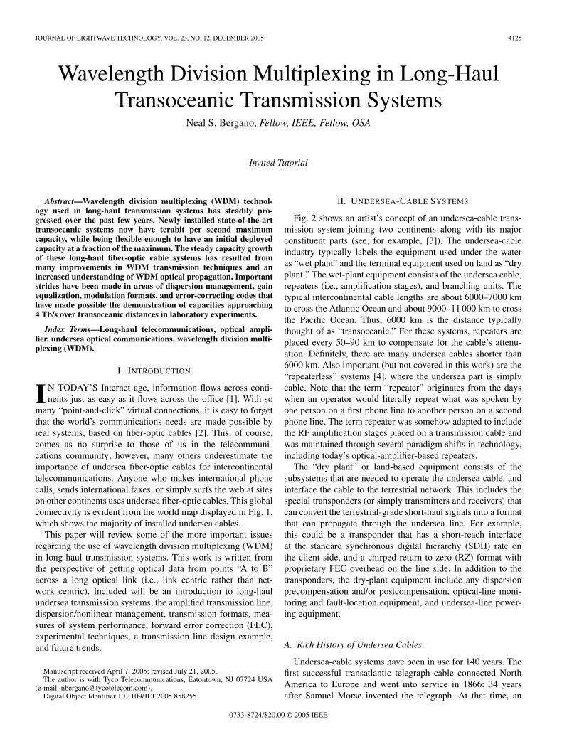
many “point-and-click” virtual connections, it is easy to forgetthat the world’s communications needs are made possible byreal systems, based on fiber-optic cables [2]. This, of course,comes as no surprise to those of us in the telecommuni-cations community; however, many others underestimate theimportance of undersea fiber-optic cables for intercontinentaltelecommunications. Anyone who makes international phonecalls, sends international faxes, or simply surfs the web at siteson other continents uses undersea fiber-optic cables. This globalconnectivity is evident from the world map displayed in Fig. 1,which shows the majority of installed undersea cables.

This paper will review some of the more important issuesregarding the use of wavelength division multiplexing (WDM)in long-haul transmission systems. This work is written fromthe perspective of getting optical data from points “A to B”across a long optical link (i.e., link centric rather than net-work centric). Included will be an introduction to long-haulundersea transmission systems, the amplified transmission line,dispersion/nonlinear management, transmission formats, mea-sures of system performance, forward error correction (FEC),experimental techniques, a transmission line design example,and future trends.

Manuscript received April 7, 2005; revised July 21, 2005.The author is with Tyco Telecommunications, Eatontown, NJ 07724 USA

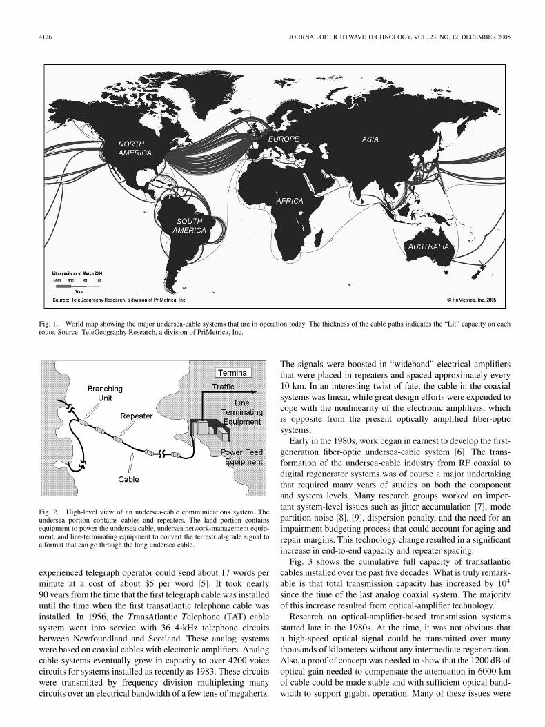
(e-mail: [email protected]).Digital Object Identifier 10.1109/JLT.2005.858255

II. UNDERSEA-CABLE SYSTEMS

Fig. 2 shows an artist’s concept of an undersea-cable trans-mission system joining two continents along with its majorconstituent parts (see, for example, [3]). The undersea-cableindustry typically labels the equipment used under the wateras “wet plant” and the terminal equipment used on land as “dryplant.” The wet-plant equipment consists of the undersea cable,repeaters (i.e., amplification stages), and branching units. Thetypical intercontinental cable lengths are about 6000–7000 kmto cross the Atlantic Ocean and about 9000–11 000 km to crossthe Pacific Ocean. Thus, 6000 km is the distance typicallythought of as “transoceanic.” For these systems, repeaters areplaced every 50–90 km to compensate for the cable’s attenu-ation. Definitely, there are many undersea cables shorter than6000 km. Also important (but not covered in this work) are the“repeaterless” systems [4], where the undersea part is simplycable. Note that the term “repeater” originates from the dayswhen an operator would literally repeat what was spoken byone person on a first phone line to another person on a secondphone line. The term repeater was somehow adapted to includethe RF amplification stages placed on a transmission cable andwas maintained through several paradigm shifts in technology,including today’s optical-amplifier-based repeaters.

The “dry plant” or land-based equipment consists of thesubsystems that are needed to operate the undersea cable, andinterface the cable to the terrestrial network. This includes thespecial transponders (or simply transmitters and receivers) thatcan convert the terrestrial-grade short-haul signals into a formatthat can propagate through the undersea line. For example,this could be a transponder that has a short-reach interfaceat the standard synchronous digital hierarchy (SDH) rate onthe client side, and a chirped return-to-zero (RZ) format withproprietary FEC overhead on the line side. In addition to thetransponders, the dry-plant equipment include any dispersionprecompensation and/or postcompensation, optical-line moni-toring and fault-location equipment, and undersea-line power-ing equipment.

A. Rich History of Undersea Cables

Undersea-cable systems have been in use for 140 years. Thefirst successful transatlantic telegraph cable connected NorthAmerica to Europe and went into service in 1866: 34 yearsafter Samuel Morse invented the telegraph. At that time, an

0733-8724/$20.00 © 2005 IEEE

4126 JOURNAL OF LIGHTWAVE TECHNOLOGY, VOL. 23, NO. 12, DECEMBER 2005

Fig. 1. World map showing the major undersea-cable systems that are in operation today. The thickness of the cable paths indicates the “Lit” capacity on eachroute. Source: TeleGeography Research, a division of PriMetrica, Inc.

Fig. 2. High-level view of an undersea-cable communications system. Theundersea portion contains cables and repeaters. The land portion containsequipment to power the undersea cable, undersea network-management equip-ment, and line-terminating equipment to convert the terrestrial-grade signal toa format that can go through the long undersea cable.

experienced telegraph operator could send about 17 words perminute at a cost of about $5 per word [5]. It took nearly90 years from the time that the first telegraph cable was installeduntil the time when the first transatlantic telephone cable wasinstalled. In 1956, the TransAtlantic Telephone (TAT) cablesystem went into service with 36 4-kHz telephone circuitsbetween Newfoundland and Scotland. These analog systemswere based on coaxial cables with electronic amplifiers. Analogcable systems eventually grew in capacity to over 4200 voicecircuits for systems installed as recently as 1983. These circuitswere transmitted by frequency division multiplexing manycircuits over an electrical bandwidth of a few tens of megahertz.

The signals were boosted in “wideband” electrical amplifiersthat were placed in repeaters and spaced approximately every10 km. In an interesting twist of fate, the cable in the coaxialsystems was linear, while great design efforts were expended tocope with the nonlinearity of the electronic amplifiers, whichis opposite from the present optically amplified fiber-opticsystems.

Early in the 1980s, work began in earnest to develop the first-generation fiber-optic undersea-cable system [6]. The trans-formation of the undersea-cable industry from RF coaxial todigital regenerator systems was of course a major undertakingthat required many years of studies on both the componentand system levels. Many research groups worked on impor-tant system-level issues such as jitter accumulation [7], modepartition noise [8], [9], dispersion penalty, and the need for animpairment budgeting process that could account for aging andrepair margins. This technology change resulted in a significantincrease in end-to-end capacity and repeater spacing.

Fig. 3 shows the cumulative full capacity of transatlanticcables installed over the past five decades. What is truly remark-able is that total transmission capacity has increased by 104

since the time of the last analog coaxial system. The majorityof this increase resulted from optical-amplifier technology.

Research on optical-amplifier-based transmission systemsstarted late in the 1980s. At the time, it was not obvious thata high-speed optical signal could be transmitted over manythousands of kilometers without any intermediate regeneration.Also, a proof of concept was needed to show that the 1200 dB ofoptical gain needed to compensate the attenuation in 6000 kmof cable could be made stable and with sufficient optical band-width to support gigabit operation. Many of these issues were

BERGANO: WAVELENGTH DIVISION MULTIPLEXING IN LONG-HAUL TRANSOCEANIC TRANSMISSION SYSTEMS 4127

Fig. 3. Full capacity of transatlantic cable systems installed over the pastfive decades, displayed in STM-1’s (or “equivalent STM-1s” for the analogsystems).

Fig. 4. Capacity of transoceanic-length transmission experiments measuredin Gb/s, and the associated technology milestones. During the 1990s, thedemonstrated capacity rapidly increased as more and more optical bandwidthwas used. The rate of increase slowed dramatically in the early 2000s when thefull EDFA bandwidth was exploited.

resolved by early transmission experiments using circulatingloops [10] and straight-line testbeds [11]. Once the undersea-cable industry transitioned to single-channel optical-amplifiersystems, research efforts focused on increasing capacity andreducing circuit cost by using WDM techniques.

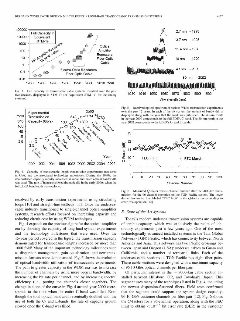
Fig. 4 expands on the previous figure for the optical-amplifierera by showing the capacity of long-haul-system experimentsand the technology milestones that were used. Over the15-year period covered in the figure, the transmission capacitydemonstrated for transoceanic lengths increased by more than1000 fold! Many of the important technology milestones suchas dispersion management, gain equalization, and new trans-mission formats were demonstrated. Fig. 5 shows the evolutionof optical-bandwidth utilization of transoceanic experiments.The path to greater capacity in the WDM era was to increasethe number of channels by using more optical bandwidth, byincreasing the bit rate per channel, and by increasing spectralefficiency (i.e., putting the channels closer together). Thechange in slope of the curve in Fig. 4 around year 2000 corre-sponds to the time when the entire C-band was filled. Eventhough the total optical bandwidth eventually doubled with theuse of both the C- and L-bands, the rate of capacity growthslowed once the C-band was filled.

Fig. 5. Received optical spectrum of various WDM transmission experimentsover the past 12 years. In each of the six curves, the amount of bandwidth isdisplayed along with the year that the work was published. The 43-nm resultin the year 2000 corresponds to the full EDFA C-band. The 80-nm result in theyear 2002 corresponds to the EDFA’s C- and L-bands.

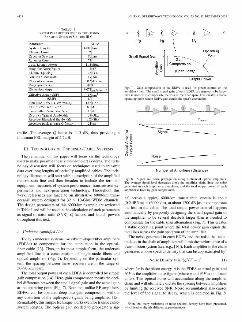
Fig. 6. Measured Q-factor versus channel number after the 9000-km trans-mission for the 96-channel operation on the TGN Pacific system. The lowerdashed horizontal line labeled “FEC limit” is the Q-factor corresponding toerror-free operation [12].

B. State-of-the-Art Systems

Today’s modern undersea transmission systems are capableof terabit capacity, which was exclusively the realm of lab-oratory experiments just a few years ago. One of the mosttechnologically advanced installed systems is the Tata GlobalNetwork (TGN) Pacific, which has connectivity between NorthAmerica and Asia. This network has two Pacific crossings be-tween Japan and Oregon (USA): undersea cables to Guam andCalifornia, and a number of terrestrial links. Each of theundersea-cable sections of TGN Pacific has eight fiber pairs.These cable sections were designed with a maximum capacityof 96 10-Gb/s optical channels per fiber pair.

Of particular interest is the ∼ 9000-km cable section in-stalled between Hillsboro, OR, and Toyohashi, Japan. Thissegment uses many of the techniques listed in Fig. 4, includingthe newest dispersion-flattened fibers. Field tests confirmedthat the segment could support the system-design capacity:96 10-Gb/s customer channels per fiber pair [12]. Fig. 6 showsthe Q-factors for a 96-channel operation, along with the FEClimit to obtain < 10−15 bit error rate (BER) in the customer


TABLE ISYSTEM PARAMETERS USED IN THE DESIGN

EXAMPLE GIVEN IN SECTION III-G

traffic. The average Q-factor is 11.3 dB, thus providing aminimum FEC margin of 2.2 dB.

III. TECHNOLOGY OF UNDERSEA-CABLE SYSTEMS

The remainder of this paper will focus on the technologyused to make possible these state-of-the-art systems. The tech-nology discussion will focus on techniques used to transmitdata over long lengths of optically amplified cables. The tech-nology discussion will start with a description of the amplifiedtransmission line and then broaden to include the terminalequipment, measures of system performance, transmission ex-periments and next-generation technology. Throughout thiswork, references are made to an illustrative 6000-km trans-oceanic system designed for 32 × 10-Gb/s WDM channels.The design parameters of this 6000-km example are reviewedin Table I and will be used in the calculation of such parametersas signal-to-noise ratio (SNR), Q-factors, and launch powersthroughout this text.

A. Undersea Amplified Line

Today’s undersea systems use erbium-doped fiber amplifiers(EDFAs) to compensate for the attenuation in the optical-fiber cable [13]. Thus, in its most simple form, the underseaamplified line is a concatenation of single-mode fibers andoptical amplifiers (Fig. 7). Depending on the particular sys-tem, the spacing between these repeaters are in the range of50–90 km apart.

The total output power of each EDFA is controlled by simplegain compression [14]. Here, gain compression means the deci-bel difference between the small signal gain and the actual gainat the operating point (Fig. 7). Note that unlike RF amplifiers,EDFAs can be operated deep into gain compression withoutany distortion of the high-speed signals being amplified [15].Remarkably, this simple technique works even for transoceanic-system lengths. The optical gain needed to propagate a sig-

Fig. 7. Gain compression in the EDFA is used for power control on theamplifier chain. The small signal gain of each EDFA is designed to be largerthan is needed to compensate the loss of the fiber span. This creates a stableoperating point where EDFA gain equals the span’s attenuation.

Fig. 8. Signal and noise propagation along a chain of optical amplifiers.The average signal level decreases along the amplifier chain since the noisegenerated in each amplifier accumulates, and the total output power of eachamplifier is fixed by gain compression.

nal across a typical 6000-km transatlantic system is about(0.2 dB/km) × (6000 km), or about 1200 dB just to compensatethe loss in the cable. The total output-power control happensautomatically by purposely designing the small signal gain ofthe amplifier to be several decibels larger than is needed tocompensate for the cable span attenuation (Fig. 7). This createsa stable operating point where the total power gain equals thetotal loss across the gain spectrum of the amplifier.

The noise generated in each EDFA and the noise that accu-mulates in the chain of amplifiers will limit the performance of atransmission system (see, e.g., [16]). Each amplifier in the chaingenerates a noise spectral density that can be approximated by1

Noise Density ≈ hν(gNF − 1) (1)

where hν is the photo energy, g is the EDFA external gain, andNF is the amplifier noise figure (where g and NF are in linearunits). This optical noise will accumulate along the amplifierchain and will ultimately dictate the spacing between amplifiersby limiting the received SNR. Noise accumulation also causesthe level of the signal to decay, which is depicted in Fig. 8.

1Note that many variations on noise spectral density have been presented,which lead to slightly different approximations.


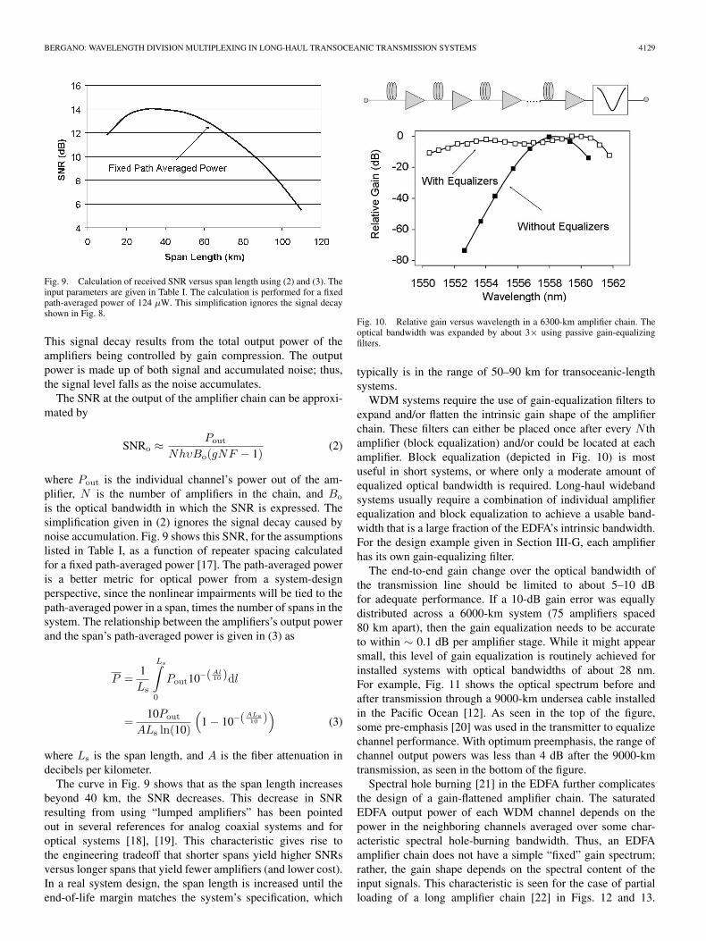
Fig. 9. Calculation of received SNR versus span length using (2) and (3). Theinput parameters are given in Table I. The calculation is performed for a fixedpath-averaged power of 124 µW. This simplification ignores the signal decayshown in Fig. 8.

This signal decay results from the total output power of theamplifiers being controlled by gain compression. The outputpower is made up of both signal and accumulated noise; thus,the signal level falls as the noise accumulates.

The SNR at the output of the amplifier chain can be approxi-mated by

SNRo ≈ Pout

NhυBo(gNF − 1)(2)

where Pout is the individual channel’s power out of the am-plifier, N is the number of amplifiers in the chain, and Bo

is the optical bandwidth in which the SNR is expressed. Thesimplification given in (2) ignores the signal decay caused bynoise accumulation. Fig. 9 shows this SNR, for the assumptionslisted in Table I, as a function of repeater spacing calculatedfor a fixed path-averaged power [17]. The path-averaged poweris a better metric for optical power from a system-designperspective, since the nonlinear impairments will be tied to thepath-averaged power in a span, times the number of spans in thesystem. The relationship between the amplifiers’s output powerand the span’s path-averaged power is given in (3) as

P =1Ls

Ls∫0

Pout10−(Al10 )dl

=10Pout

ALs ln(10)

(1 − 10−(ALs

10 ))

(3)

where Ls is the span length, and A is the fiber attenuation indecibels per kilometer.

The curve in Fig. 9 shows that as the span length increasesbeyond 40 km, the SNR decreases. This decrease in SNRresulting from using “lumped amplifiers” has been pointedout in several references for analog coaxial systems and foroptical systems [18], [19]. This characteristic gives rise tothe engineering tradeoff that shorter spans yield higher SNRsversus longer spans that yield fewer amplifiers (and lower cost).In a real system design, the span length is increased until theend-of-life margin matches the system’s specification, which

Fig. 10. Relative gain versus wavelength in a 6300-km amplifier chain. Theoptical bandwidth was expanded by about 3× using passive gain-equalizingfilters.

typically is in the range of 50–90 km for transoceanic-lengthsystems.

WDM systems require the use of gain-equalization filters toexpand and/or flatten the intrinsic gain shape of the amplifierchain. These filters can either be placed once after every N thamplifier (block equalization) and/or could be located at eachamplifier. Block equalization (depicted in Fig. 10) is mostuseful in short systems, or where only a moderate amount ofequalized optical bandwidth is required. Long-haul widebandsystems usually require a combination of individual amplifierequalization and block equalization to achieve a usable band-width that is a large fraction of the EDFA’s intrinsic bandwidth.For the design example given in Section III-G, each amplifierhas its own gain-equalizing filter.

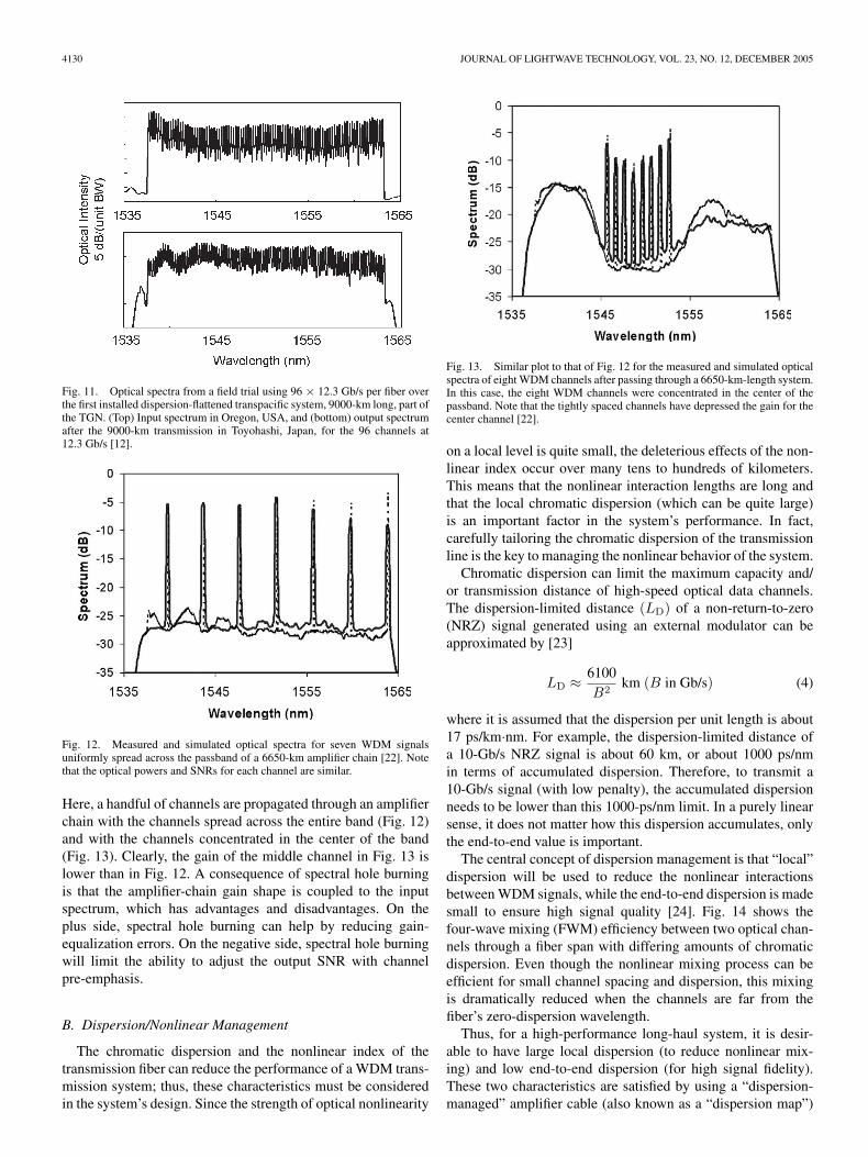
The end-to-end gain change over the optical bandwidth ofthe transmission line should be limited to about 5–10 dBfor adequate performance. If a 10-dB gain error was equallydistributed across a 6000-km system (75 amplifiers spaced80 km apart), then the gain equalization needs to be accurateto within ∼ 0.1 dB per amplifier stage. While it might appearsmall, this level of gain equalization is routinely achieved forinstalled systems with optical bandwidths of about 28 nm.For example, Fig. 11 shows the optical spectrum before andafter transmission through a 9000-km undersea cable installedin the Pacific Ocean [12]. As seen in the top of the figure,some pre-emphasis [20] was used in the transmitter to equalizechannel performance. With optimum preemphasis, the range ofchannel output powers was less than 4 dB after the 9000-kmtransmission, as seen in the bottom of the figure.

Spectral hole burning [21] in the EDFA further complicatesthe design of a gain-flattened amplifier chain. The saturatedEDFA output power of each WDM channel depends on thepower in the neighboring channels averaged over some char-acteristic spectral hole-burning bandwidth. Thus, an EDFAamplifier chain does not have a simple “fixed” gain spectrum;rather, the gain shape depends on the spectral content of theinput signals. This characteristic is seen for the case of partialloading of a long amplifier chain [22] in Figs. 12 and 13.


Fig. 11. Optical spectra from a field trial using 96 × 12.3 Gb/s per fiber overthe first installed dispersion-flattened transpacific system, 9000-km long, part ofthe TGN. (Top) Input spectrum in Oregon, USA, and (bottom) output spectrumafter the 9000-km transmission in Toyohashi, Japan, for the 96 channels at12.3 Gb/s [12].

Fig. 12. Measured and simulated optical spectra for seven WDM signalsuniformly spread across the passband of a 6650-km amplifier chain [22]. Notethat the optical powers and SNRs for each channel are similar.

Here, a handful of channels are propagated through an amplifierchain with the channels spread across the entire band (Fig. 12)and with the channels concentrated in the center of the band(Fig. 13). Clearly, the gain of the middle channel in Fig. 13 islower than in Fig. 12. A consequence of spectral hole burningis that the amplifier-chain gain shape is coupled to the inputspectrum, which has advantages and disadvantages. On theplus side, spectral hole burning can help by reducing gain-equalization errors. On the negative side, spectral hole burningwill limit the ability to adjust the output SNR with channelpre-emphasis.

B. Dispersion/Nonlinear Management

The chromatic dispersion and the nonlinear index of thetransmission fiber can reduce the performance of a WDM trans-mission system; thus, these characteristics must be consideredin the system’s design. Since the strength of optical nonlinearity

Fig. 13. Similar plot to that of Fig. 12 for the measured and simulated opticalspectra of eight WDM channels after passing through a 6650-km-length system.In this case, the eight WDM channels were concentrated in the center of thepassband. Note that the tightly spaced channels have depressed the gain for thecenter channel [22].

on a local level is quite small, the deleterious effects of the non-linear index occur over many tens to hundreds of kilometers.This means that the nonlinear interaction lengths are long andthat the local chromatic dispersion (which can be quite large)is an important factor in the system’s performance. In fact,carefully tailoring the chromatic dispersion of the transmissionline is the key to managing the nonlinear behavior of the system.

Chromatic dispersion can limit the maximum capacity and/or transmission distance of high-speed optical data channels.The dispersion-limited distance (LD) of a non-return-to-zero(NRZ) signal generated using an external modulator can beapproximated by [23]

LD ≈ 6100B2

km (B in Gb/s) (4)

where it is assumed that the dispersion per unit length is about17 ps/km·nm. For example, the dispersion-limited distance ofa 10-Gb/s NRZ signal is about 60 km, or about 1000 ps/nmin terms of accumulated dispersion. Therefore, to transmit a10-Gb/s signal (with low penalty), the accumulated dispersionneeds to be lower than this 1000-ps/nm limit. In a purely linearsense, it does not matter how this dispersion accumulates, onlythe end-to-end value is important.

The central concept of dispersion management is that “local”dispersion will be used to reduce the nonlinear interactionsbetween WDM signals, while the end-to-end dispersion is madesmall to ensure high signal quality [24]. Fig. 14 shows thefour-wave mixing (FWM) efficiency between two optical chan-nels through a fiber span with differing amounts of chromaticdispersion. Even though the nonlinear mixing process can beefficient for small channel spacing and dispersion, this mixingis dramatically reduced when the channels are far from thefiber’s zero-dispersion wavelength.

Thus, for a high-performance long-haul system, it is desir-able to have large local dispersion (to reduce nonlinear mix-ing) and low end-to-end dispersion (for high signal fidelity).These two characteristics are satisfied by using a “dispersion-managed” amplifier cable (also known as a “dispersion map”)


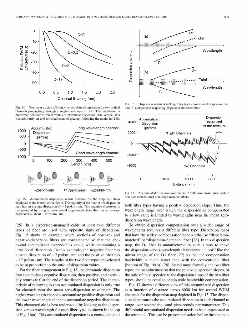
Fig. 14. Nonlinear mixing efficiency verses channel separation for two opticalchannels propagating through a single-mode optical fiber. The calculation ispreformed for four different values of chromatic dispersion. The vertical axiswas arbitrarily set to 0 for small channel spacing (following the model in [24]).

Fig. 15. Accumulated dispersion versus distance for the amplifier chaindisplayed in the bottom of the figure. The majority of the fiber in this dispersionmap has an average dispersion of −2 ps/km · nm. This negative dispersion iscompensated by using a conventional single-mode fiber that has an averagedispersion of about +17 ps/km · nm.

[25]. In a dispersion-managed cable at least two differenttypes of fiber are used with opposite signs of dispersion.Fig. 15 shows an example where sections of positive- andnegative-dispersion fibers are concatenated so that the end-to-end accumulated dispersion is small, while maintaining alarge local dispersion. In this example, the negative fiber hasa mean dispersion of −2 ps/km · nm and the positive fiber has+17 ps/km · nm. The lengths of the two fiber types are selectedto be in proportion to the ratio of dispersion values.

For the fiber arrangement in Fig. 15, the chromatic dispersionfirst accumulates negative dispersion, then positive, and eventu-ally returns to 0 at the end of the dispersion period. The charac-teristic of returning to zero accumulated dispersion is only truefor channels near the mean zero-dispersion wavelength. Thehigher wavelength channels accumulate positive dispersion andthe lower wavelength channels accumulate negative dispersion.This characteristic is best understood by looking at the disper-sion versus wavelength for each fiber type, as shown in the topof Fig. 16(a). This accumulated dispersion is a consequence of

Fig. 16. Dispersion versus wavelength for (a) a conventional dispersion mapand (b) a dispersion map using dispersion-flattened fiber.

Fig. 17. Accumulated dispersion over an entire 6000-km transmission systemthat uses conventional non-slope-matched fibers.

both fiber types having a positive dispersion slope. Thus, thewavelength range over which the dispersion is compensatedto a low value is limited to wavelengths near the mean zero-dispersion wavelength.

To obtain dispersion compensation over a wider range ofwavelengths requires a different fiber type. Dispersion mapsthat have the widest compensation bandwidths use “dispersion-matched” or “dispersion-flattened” fiber [26]. In this dispersionmap, the D- fiber is manufactured in such a way to makethe dispersion-versus-wavelength characteristic “look” like themirror image of the D+ fiber [27] so that the compensationbandwidth is much larger than with the conventional fiber[bottom of Fig. 16(b)] [28]. Stated more formally, the two fibertypes are manufactured so that the relative dispersion slopes, orthe ratio of the dispersion to the dispersion slope of the two fibertypes, should be equal to obtain wide bandwidth compensation.

Fig. 17 shows a different view of this accumulated dispersionas a function of distance across 6000 km for several WDMchannels for the dispersion map depicted in Fig. 15. The disper-sion slope causes the accumulated dispersion in each channel torange over several thousand picoseconds per nanometer. Thisdifferential accumulated dispersion needs to be compensated atthe terminals. This can be precompensation before the channels


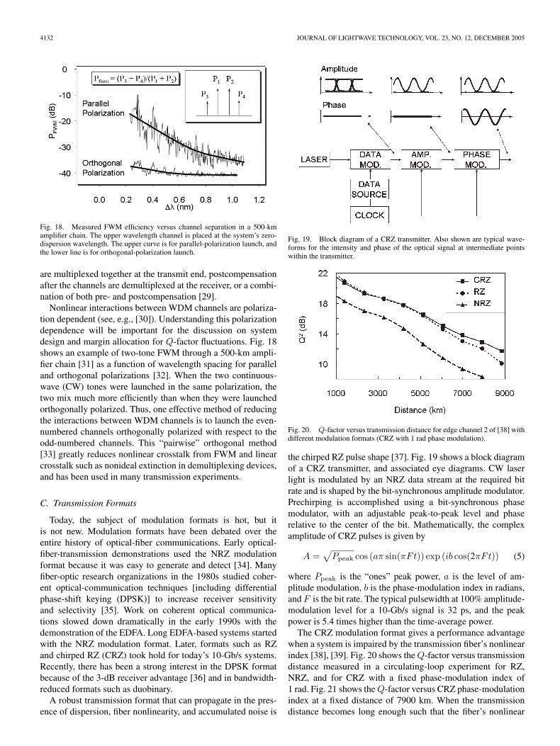
Fig. 18. Measured FWM efficiency versus channel separation in a 500-kmamplifier chain. The upper wavelength channel is placed at the system’s zero-dispersion wavelength. The upper curve is for parallel-polarization launch, andthe lower line is for orthogonal-polarization launch.

are multiplexed together at the transmit end, postcompensationafter the channels are demultiplexed at the receiver, or a combi-nation of both pre- and postcompensation [29].

Nonlinear interactions between WDM channels are polariza-tion dependent (see, e.g., [30]). Understanding this polarizationdependence will be important for the discussion on systemdesign and margin allocation for Q-factor fluctuations. Fig. 18shows an example of two-tone FWM through a 500-km ampli-fier chain [31] as a function of wavelength spacing for paralleland orthogonal polarizations [32]. When the two continuous-wave (CW) tones were launched in the same polarization, thetwo mix much more efficiently than when they were launchedorthogonally polarized. Thus, one effective method of reducingthe interactions between WDM channels is to launch the even-numbered channels orthogonally polarized with respect to theodd-numbered channels. This “pairwise” orthogonal method[33] greatly reduces nonlinear crosstalk from FWM and linearcrosstalk such as nonideal extinction in demultiplexing devices,and has been used in many transmission experiments.

C. Transmission Formats

Today, the subject of modulation formats is hot, but itis not new. Modulation formats have been debated over theentire history of optical-fiber communications. Early optical-fiber-transmission demonstrations used the NRZ modulationformat because it was easy to generate and detect [34]. Manyfiber-optic research organizations in the 1980s studied coher-ent optical-communication techniques [including differentialphase-shift keying (DPSK)] to increase receiver sensitivityand selectivity [35]. Work on coherent optical communica-tions slowed down dramatically in the early 1990s with thedemonstration of the EDFA. Long EDFA-based systems startedwith the NRZ modulation format. Later, formats such as RZand chirped RZ (CRZ) took hold for today’s 10-Gb/s systems.Recently, there has been a strong interest in the DPSK formatbecause of the 3-dB receiver advantage [36] and in bandwidth-reduced formats such as duobinary.

A robust transmission format that can propagate in the pres-ence of dispersion, fiber nonlinearity, and accumulated noise is

Fig. 19. Block diagram of a CRZ transmitter. Also shown are typical wave-forms for the intensity and phase of the optical signal at intermediate pointswithin the transmitter.

Fig. 20. Q-factor versus transmission distance for edge channel 2 of [38] withdifferent modulation formats (CRZ with 1 rad phase modulation).

the chirped RZ pulse shape [37]. Fig. 19 shows a block diagramof a CRZ transmitter, and associated eye diagrams. CW laserlight is modulated by an NRZ data stream at the required bitrate and is shaped by the bit-synchronous amplitude modulator.Prechirping is accomplished using a bit-synchronous phasemodulator, with an adjustable peak-to-peak level and phaserelative to the center of the bit. Mathematically, the complexamplitude of CRZ pulses is given by

A =√

Ppeak cos (aπ sin(πFt)) exp (ib cos(2πFt)) (5)

where Ppeak is the “ones” peak power, a is the level of am-plitude modulation, b is the phase-modulation index in radians,and F is the bit rate. The typical pulsewidth at 100% amplitude-modulation level for a 10-Gb/s signal is 32 ps, and the peakpower is 5.4 times higher than the time-average power.

The CRZ modulation format gives a performance advantagewhen a system is impaired by the transmission fiber’s nonlinearindex [38], [39]. Fig. 20 shows the Q-factor versus transmissiondistance measured in a circulating-loop experiment for RZ,NRZ, and for CRZ with a fixed phase-modulation index of1 rad. Fig. 21 shows the Q-factor versus CRZ phase-modulationindex at a fixed distance of 7900 km. When the transmissiondistance becomes long enough such that the fiber’s nonlinear


Fig. 21. Q-factor versus phase-modulation index for channel 2 [38] at7900 km, employing CRZ.

behavior starts to limit the performance of the standard RZformat, the CRZ format has a performance advantage (at theexpense of using more optical bandwidth).

A simplified explanation of this improvement can be givenin either the time or the frequency domains. In the time-domainargument, the added bandwidth given by the phase modulationcoupled with the fiber’s dispersion spreads the data pulsesover many bits, thus quickly changing the signal intensityand averaging nonlinear phase shift for different time samplesof the signal. This fast intensity evolution of the signal withdistance lowers not only self-phase-modulation effects in thesame channel but nonlinear interaction between neighboringchannels as well. In the frequency-domain argument, the phasemodulation spreads the spectrum of the signal, thus reducingthe peak amplitude of any particular Fourier component. Thesereduced spectral peaks lowers nonlinear mixing between spec-tral components of other data signals or noise components, thusimproving nonlinear tolerance.

D. Measures of System Performance

The performance of a digital transmission system is specifiedin terms of the Q-factor [40]. The Q-factor is an equivalentelectrical SNR at the input to the receiver that dictates thereceived BER. This SNR is depicted in Fig. 22, which showsa typical eye diagram with a voltage histogram at the samplingpoint. The upper and lower lobes of the distribution havean associated mean and standard deviation that are used todefine the Q-factor given in (6). The Q-factor describes theperformance of the entire transmission path from the opticaltransmitter, through the optical path, and into the receiver. TheQ-factor was adapted from Personick’s work on calculatingthe performance of receivers in lightwave links [41]. TheQ-factor has become the standard parameter used to accountfor the various impairments in the design process of optical-amplifier systems and is used in the “impairment budget” givenin Table II for the 32 × 10-Gb/s WDM example.

q ≡(|µ1 − µ0|σ1 + σ0

)(6)

Fig. 22. Typical RZ eye diagram at the input to a decision circuit. The voltagesamples that fall within the sampling window are used to form the histogram onthe right-hand side. The upper and lower lobes of the voltage histogram havean associated mean and standard deviation.

TABLE IITYPICAL IMPAIRMENT BUDGET FOR THE 6000-km

TRANSMISSION-SYSTEM EXAMPLE GIVEN IN TABLE I

The Q-factor is related to the system’s BER through the com-plementary error function erfc() given by

BER(q) =12erfc

(q√2

)=

1√2π

∞∫q

e−α22 dα

where erfc(x) =2√π

∞∫x

e−α2dα (7)

or in terms of the more standard error function erf()

BER(q) =12

[1 − erf

(q√2

)]

where erf(x) =2√π

x∫0

e−α2dα. (8)

It is often useful to have numerical approximations tocalculate BER from Q-factor [42] and Q-factor from BER.These approximations are given in (9) and (10).

BER ≈ e−q2

2

q√

2π− e−

q2

2

q√

2π(q2 + 2)+

e−q2

2

q√

2π(q2 + 2)(q2 + 4)

− 5e−q2

2

q√

2π(q2 + 2)(q2 + 4)(q2 + 6)+ · · · (9)


Note that the first term in (9) is the typical approximationused in many publications. Equation (9) also includes the nextfew higher order terms that are needed for a more accurateestimation, which is important when calculating BERs for lowQ-factors, which are now typical for experiments with strongFEC. For example, using only the first term of (9) gives > 10%error for Q-factors less than ∼ 9.5 dB, whereas including allthe terms gives an estimate better than 1% down to a Q-factorof 3 dB.

Equation (10) gives an approximation for the reverse opera-tion of estimating Q-factor from BER [43].

Let t =√−2Ln(BER)

q ≈ t −[

2.515517 + 0.802853t + 0.010328t2

1 + 1.432788t + 0.189269t2 + 0.001308t3

].

(10)

In (6)–(10), the Q-factor is expressed as a unitless ratiodenoted by a lower case “q.” Often, it is more convenientto express Q-factor in decibels as 20Log(q). The factor of20 (or 10Log(q2)) is used to maintain consistency with thelinear noise-accumulation model. For example, a 3-dB increasein the average launch power in all of the spans results in a 3-dBincrease in Q-factor (assuming signal-spontaneous beat noisedominates, and ignoring signal decay and fiber nonlinearity).

There are several ways to experimentally estimate theQ-factor of an optical transmission system based on BER,eye diagrams, and/or optical SNR (OSNR). It is desirableto have an estimate of Q-factor based on a measurement ofBER. One difficulty using BER is that often, the line side ofa transmission system runs “error free.” In this case, othermethods are required, such as using the decision-circuit methodof estimating Q-factor, as described in [40], and in InternationalTelecommunication Union (ITU) publication O.201 [44]. Thedirect measurement of line-side BER is made easier in modernoptical systems that have FEC-enhanced terminals, as will bediscussed next.

E. Error Correcting Codes

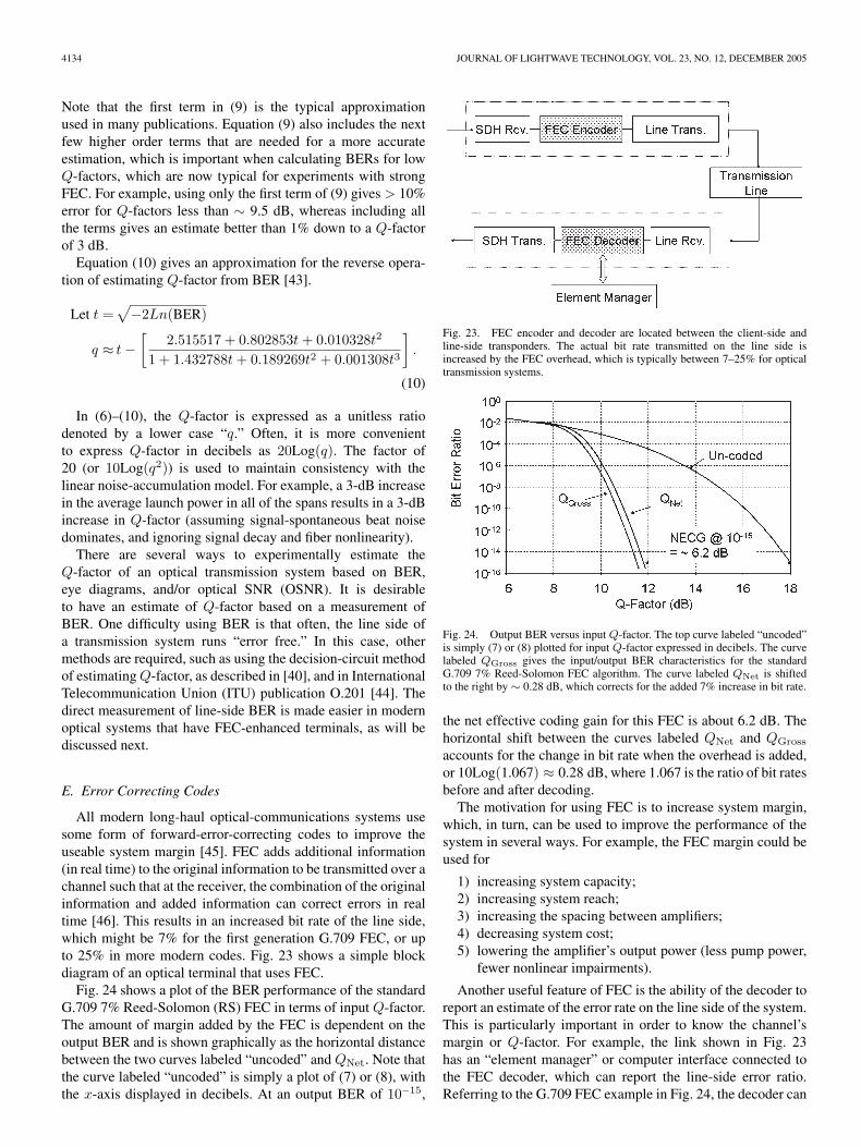
All modern long-haul optical-communications systems usesome form of forward-error-correcting codes to improve theuseable system margin [45]. FEC adds additional information(in real time) to the original information to be transmitted over achannel such that at the receiver, the combination of the originalinformation and added information can correct errors in realtime [46]. This results in an increased bit rate of the line side,which might be 7% for the first generation G.709 FEC, or upto 25% in more modern codes. Fig. 23 shows a simple blockdiagram of an optical terminal that uses FEC.

Fig. 24 shows a plot of the BER performance of the standardG.709 7% Reed-Solomon (RS) FEC in terms of input Q-factor.The amount of margin added by the FEC is dependent on theoutput BER and is shown graphically as the horizontal distancebetween the two curves labeled “uncoded” and QNet. Note thatthe curve labeled “uncoded” is simply a plot of (7) or (8), withthe x-axis displayed in decibels. At an output BER of 10−15,

Fig. 23. FEC encoder and decoder are located between the client-side andline-side transponders. The actual bit rate transmitted on the line side isincreased by the FEC overhead, which is typically between 7–25% for opticaltransmission systems.

Fig. 24. Output BER versus input Q-factor. The top curve labeled “uncoded”is simply (7) or (8) plotted for input Q-factor expressed in decibels. The curvelabeled QGross gives the input/output BER characteristics for the standardG.709 7% Reed-Solomon FEC algorithm. The curve labeled QNet is shiftedto the right by ∼ 0.28 dB, which corrects for the added 7% increase in bit rate.

the net effective coding gain for this FEC is about 6.2 dB. Thehorizontal shift between the curves labeled QNet and QGross

accounts for the change in bit rate when the overhead is added,or 10Log(1.067) ≈ 0.28 dB, where 1.067 is the ratio of bit ratesbefore and after decoding.

The motivation for using FEC is to increase system margin,which, in turn, can be used to improve the performance of thesystem in several ways. For example, the FEC margin could beused for

1) increasing system capacity;2) increasing system reach;3) increasing the spacing between amplifiers;4) decreasing system cost;5) lowering the amplifier’s output power (less pump power,

fewer nonlinear impairments).

Another useful feature of FEC is the ability of the decoder toreport an estimate of the error rate on the line side of the system.This is particularly important in order to know the channel’smargin or Q-factor. For example, the link shown in Fig. 23has an “element manager” or computer interface connected tothe FEC decoder, which can report the line-side error ratio.Referring to the G.709 FEC example in Fig. 24, the decoder can


Fig. 25. Top: Block diagram for a circulating-loop experiment. Bottom:Timing diagram for a circulating-loop measurement showing the optical switchstates and the time gate for making measurements.

directly measure the line BER in the range of 10−5 to 10−15,while the client side runs error free.

F. Transmission-Experiment Techniques

Transmission experiments are an important part of thesystem-design process. This is especially true when new tech-nologies and/or techniques are being introduced for the firsttime. For example, using EDFAs in undersea-cable systemsis obvious today; however, in 1990, it was not obvious thatan EDFA-based amplifier chain would work in a long cablesystem. Circulating-loop transmission experiments providedthe first proof of concept that an amplifier chain based onEDFAs could be made stable and could support a high-speedoptical channel over transoceanic distances [47]. Later, longamplifier chains were constructed to make full-length testbedsto demonstrate the feasibility of using EDFAs in optical trans-mission systems [11].

Most long-haul transmission experiments using optical am-plifiers fall into one of three categories, including circulatingloops, straight-line testbeds, and special measurements per-formed on installed systems [48]. Circulating-loop transmissionmeasurements are, by far, the most important experimentaltechnique. Circulating-loop techniques, applied to an amplifierchain of modest length, can provide an experimental platformto study a broad range of transmission phenomena for EDFA-based transmission systems.

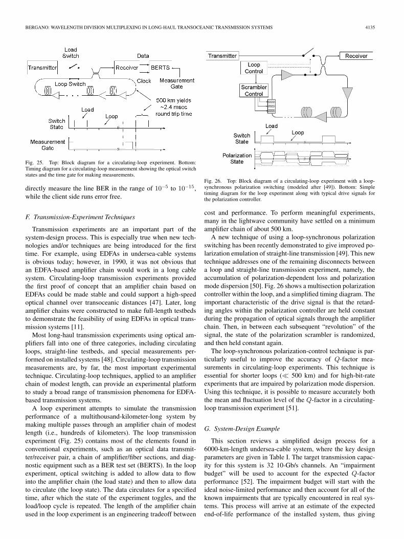
A loop experiment attempts to simulate the transmissionperformance of a multithousand-kilometer-long system bymaking multiple passes through an amplifier chain of modestlength (i.e., hundreds of kilometers). The loop transmissionexperiment (Fig. 25) contains most of the elements found inconventional experiments, such as an optical data transmit-ter/receiver pair, a chain of amplifier/fiber sections, and diag-nostic equipment such as a BER test set (BERTS). In the loopexperiment, optical switching is added to allow data to flowinto the amplifier chain (the load state) and then to allow datato circulate (the loop state). The data circulates for a specifiedtime, after which the state of the experiment toggles, and theload/loop cycle is repeated. The length of the amplifier chainused in the loop experiment is an engineering tradeoff between

Fig. 26. Top: Block diagram of a circulating-loop experiment with a loop-synchronous polarization switching (modeled after [49]). Bottom: Simpletiming diagram for the loop experiment along with typical drive signals forthe polarization controller.

cost and performance. To perform meaningful experiments,many in the lightwave community have settled on a minimumamplifier chain of about 500 km.

A new technique of using a loop-synchronous polarizationswitching has been recently demonstrated to give improved po-larization emulation of straight-line transmission [49]. This newtechnique addresses one of the remaining disconnects betweena loop and straight-line transmission experiment, namely, theaccumulation of polarization-dependent loss and polarizationmode dispersion [50]. Fig. 26 shows a multisection polarizationcontroller within the loop, and a simplified timing diagram. Theimportant characteristic of the drive signal is that the retard-ing angles within the polarization controller are held constantduring the propagation of optical signals through the amplifierchain. Then, in between each subsequent “revolution” of thesignal, the state of the polarization scrambler is randomized,and then held constant again.

The loop-synchronous polarization-control technique is par-ticularly useful to improve the accuracy of Q-factor mea-surements in circulating-loop experiments. This technique isessential for shorter loops ( 500 km) and for high-bit-rateexperiments that are impaired by polarization mode dispersion.Using this technique, it is possible to measure accurately boththe mean and fluctuation level of the Q-factor in a circulating-loop transmission experiment [51].

G. System-Design Example

This section reviews a simplified design process for a6000-km-length undersea-cable system, where the key designparameters are given in Table I. The target transmission capac-ity for this system is 32 10-Gb/s channels. An “impairmentbudget” will be used to account for the expected Q-factorperformance [52]. The impairment budget will start with theideal noise-limited performance and then account for all of theknown impairments that are typically encountered in real sys-tems. This process will arrive at an estimate of the expectedend-of-life performance of the installed system, thus giving


an estimate of the operating margin. The design process goesas follows.

1) Determine the performance of the terminal equipment toobtain the minimum Q-factor at the receiver’s input forerror-free operation (after the FEC decoder).

2) Make an educated guess for the total margin above theterminal’s FEC limit for “noise-limited” operation.

3) Design the amplifier chain over a range of repeater gains(i.e., span lengths).

4) Estimate output power and noise figure given a max pumppower, channel spacing, and wavelength range.

5) Calculate the noise-limited performance and select a spanlength and output power.

6) Perform nonlinear signal-propagation modeling to esti-mate actual performance.

7) Populate the impairment budget with realistic margins.8) Iterate to a solution.

As a starting point, it is assumed that the FEC performancegives an error-free point at an input Q-factor of about 8.5 dB,assuming a 23% overhead concatenated RS code [26]. Onto this8.5-dB target, 6.5 dB is added as an initial guess for the totalamount of margin needed over and above the FEC threshold,which gives a starting point of 15 dB mean Q-factor target. This15-dB value appears in line 1 of the impairment budget givenin Table II.

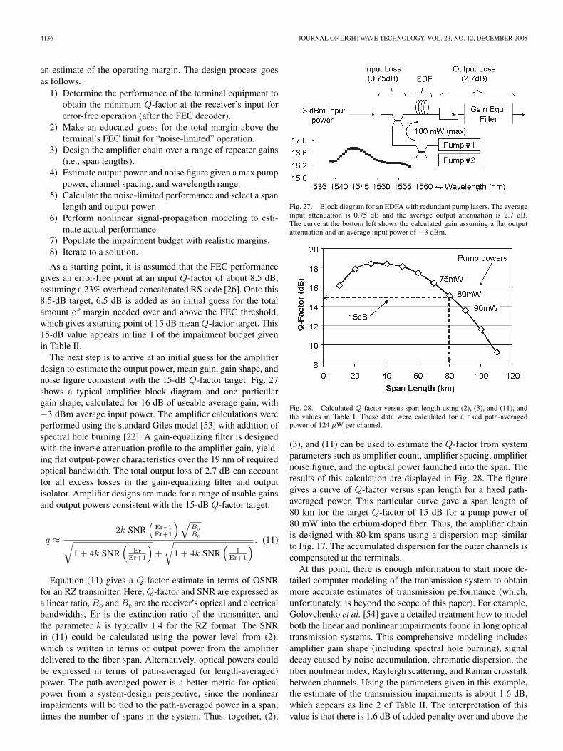
The next step is to arrive at an initial guess for the amplifierdesign to estimate the output power, mean gain, gain shape, andnoise figure consistent with the 15-dB Q-factor target. Fig. 27shows a typical amplifier block diagram and one particulargain shape, calculated for 16 dB of useable average gain, with−3 dBm average input power. The amplifier calculations wereperformed using the standard Giles model [53] with addition ofspectral hole burning [22]. A gain-equalizing filter is designedwith the inverse attenuation profile to the amplifier gain, yield-ing flat output-power characteristics over the 19 nm of requiredoptical bandwidth. The total output loss of 2.7 dB can accountfor all excess losses in the gain-equalizing filter and outputisolator. Amplifier designs are made for a range of usable gainsand output powers consistent with the 15-dB Q-factor target.

q ≈2k SNR

(Er−1Er+1

) √BoBe√

1 + 4k SNR(

ErEr+1

)+

√1 + 4k SNR

(1

Er+1

) . (11)

Equation (11) gives a Q-factor estimate in terms of OSNRfor an RZ transmitter. Here, Q-factor and SNR are expressed asa linear ratio, Bo and Be are the receiver’s optical and electricalbandwidths, Er is the extinction ratio of the transmitter, andthe parameter k is typically 1.4 for the RZ format. The SNRin (11) could be calculated using the power level from (2),which is written in terms of output power from the amplifierdelivered to the fiber span. Alternatively, optical powers couldbe expressed in terms of path-averaged (or length-averaged)power. The path-averaged power is a better metric for opticalpower from a system-design perspective, since the nonlinearimpairments will be tied to the path-averaged power in a span,times the number of spans in the system. Thus, together, (2),

Fig. 27. Block diagram for an EDFA with redundant pump lasers. The averageinput attenuation is 0.75 dB and the average output attenuation is 2.7 dB.The curve at the bottom left shows the calculated gain assuming a flat outputattenuation and an average input power of −3 dBm.

Fig. 28. Calculated Q-factor versus span length using (2), (3), and (11), andthe values in Table I. These data were calculated for a fixed path-averagedpower of 124 µW per channel.

(3), and (11) can be used to estimate the Q-factor from systemparameters such as amplifier count, amplifier spacing, amplifiernoise figure, and the optical power launched into the span. Theresults of this calculation are displayed in Fig. 28. The figuregives a curve of Q-factor versus span length for a fixed path-averaged power. This particular curve gave a span length of80 km for the target Q-factor of 15 dB for a pump power of80 mW into the erbium-doped fiber. Thus, the amplifier chainis designed with 80-km spans using a dispersion map similarto Fig. 17. The accumulated dispersion for the outer channels iscompensated at the terminals.

At this point, there is enough information to start more de-tailed computer modeling of the transmission system to obtainmore accurate estimates of transmission performance (which,unfortunately, is beyond the scope of this paper). For example,Golovchenko et al. [54] gave a detailed treatment how to modelboth the linear and nonlinear impairments found in long opticaltransmission systems. This comprehensive modeling includesamplifier gain shape (including spectral hole burning), signaldecay caused by noise accumulation, chromatic dispersion, thefiber nonlinear index, Rayleigh scattering, and Raman crosstalkbetween channels. Using the parameters given in this example,the estimate of the transmission impairments is about 1.6 dB,which appears as line 2 of Table II. The interpretation of thisvalue is that there is 1.6 dB of added penalty over and above the


Fig. 29. Block diagram of a DPSK receiver, along with typical eye diagramsat intermediate points within the receiver. The eye diagrams were measuredafter 11 000 km [58].

performance predicted by the simple noise-accumulation theoryof (2), (3), and (11).

Line 3 in the impairment budget allocates 0.5 dB for theterminal’s implementation (i.e., transmitters and receivers), de-parting from the ideal performance. For example, the wave-lengths can drift in the transmitter’s laser and/or the receiver’sfilter and the decision point in the receiver can depart fromthe ideal. Line 4 in the impairment budget allocates 1.0 dBfor the real manufacturing process, where statistical variationson the parts and the variability in the way the parts are assem-bled are considered.

Line 5 in the impairment budget allocates 1.0 dB for Q-factorvariations. Standard telecommunications fibers do not maintainthe state of polarization. Changes in the signal’s polarizationcoupled with polarization dependence in the amplifier chainwill cause the received BER to fluctuate with time [55]. Polar-ization drifts caused by temperature and/or pressure changescan be slow, or polarization changes caused by moving fibers inthe terminal can be fast. Thus, line 5 accounts for these fluctua-tions by allotting 1 dB of margin for Q-factor fluctuations.

Line 6 (the difference between line 1 and the sum oflines 2–5) is the worst-case Q-factor that would be observedusing a perfect receiver. Translating this to a Q-factor observedwith a real receiver required the introduction of a new param-eter, namely, the receiver “back-to-back” Q-factor. Equation(12) gives a simple relationship between the observed, line (orideal), and the back-to-back Q-factors as

1q2Observed

=1

q2bb

+1

q2line

(12)

where all the Q-factors are expressed as a linear ratio. Finally,an allotment of 1 dB is made for the system’s aging andrepair, which brings the expected end-of-life Q-factor to 9.5 dB(line 10). This end-of-life value measured against the FECtarget of 8.5 dB gives an end-of-life margin of 1 dB.

At this point, the entire process could be iterated to drivethe end-of-life margin to a lower number. For example, thenoise-limited Q-factor could be lowered by reducing the path-

averaged power in the transmission span. This, in turn, wouldlower the nonlinear penalty, thus changing the values in thedesign.

H. Future Trends

In today’s market where low “first cost” is important, it isessential to have a comprehensive understanding of long-hauloptical propagation than ever before. In the next generationof systems, lower first cost will be achieved by improvedequipment performance and by designing systems closer tothe margin limits. This will require a comprehensive system-level understanding of signal generation and detection in theterminals and optical propagation in the wet-plant equipment.This improved understanding will be achieved by a mix oftransmission experiments and computer simulations.

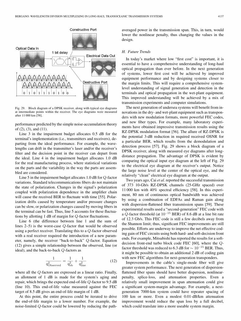
The next generation of undersea systems will benefit from in-novations in the dry- and wet-plant equipment such as transpon-ders with new modulation formats, more powerful FEC codes,and new fiber types. For example, many laboratory experi-ments have obtained impressive transmission results using theRZ-DPSK modulation format [56]. The allure of RZ-DPSK isthe potential 3-dB reduction in required received OSNR fora particular BER, which results from the demodulation anddetection process [57]. Fig. 29 shows a block diagram of aDPSK receiver, along with measured eye diagrams after long-distance propagation. The advantage of DPSK is evident bycomparing the optical input eye diagram at the left of Fig. 29to the electrical eye diagram at the receiver’s output. Noticethe large noise level at the center of the optical eye, and therelatively “clean” electrical eye diagram at the output.

Two years ago, Cai et al. reported the successful transmissionof 373 10-Gb/s RZ-DPSK channels (25-GHz spaced) over11 000 km with 40% spectral efficiency [58]. In this experi-ment, 80 nm of continuous optical bandwidth was achievedby using a combination of EDFAs and Raman gain alongwith dispersion-flattened fiber transmission spans [59]. Theseexperimental results used a “second-generation” FEC code witha Q-factor threshold (at 10−15 BER) of 8.6 dB at a line bit rateof 12.3 Gb/s. This FEC code is still a few decibels away fromthe Shannon limit; thus, significant FEC improvements are stillpossible. Efforts are underway to improve the net effective cod-ing gain of FEC circuits using both hard- and soft-decision frontends. For example, Mitsubishi has reported the results for a soft-decision front-end turbo block code FEC [60], where the Q-factor threshold was reduced to 6.3 dB for ∼ 10−15 BER. Thus,it might be possible to obtain an additional 2 dB of coding gainwith new FEC algorithms for next-generation transponders.

Improvements in the cable’s single-mode fiber will givegreater system performance. The next generation of dispersion-flattened fiber spans should have better dispersion, nonlinear-penalty, splice-loss, and attenuation properties. Even arelatively small improvement in span attenuation could givea significant system-margin advantage. For example, a next-generation 7000-km system could have repeater spacing of100 km or more. Even a modest 0.01-dB/km attenuationimprovement would reduce the span loss by a full decibel,which could translate into a more useable system margin.


In the future, Raman amplification might find more appli-cations in undersea systems (see, e.g., [61]). Today, Ramanamplification is being used in a limited roll to extend thereach of the longest repeaterless links. Going forward, Ramanamplification could be used to either augment and/or replacethe EDFA gain. For example, Ma et al. demonstrated a 240-km“repeater” spacing for a 5280-km transmission distance byusing a combination of conventional EDFAs, remote EDFAs,and Raman amplification [62]. In another demonstration,Nissov et al. demonstrated a system where the majority of theoptical gain was provided by distributed Raman gain [63]. Thenoise performance of the Raman amplifier chain was about2 dB better than a similar amplifier chain using EDFAs. What isobserved from the most recent long-haul Raman-amplificationdemonstrations is the subtle coupling between optimizing gainand the dispersion map when designing Raman spans [64].

IV. CONCLUSION

The technology used in undersea transmission systems hassteadily progressed, even though the current demand for newcable systems has been low. New state-of-the-art transoceanicsystems have terabit per second maximum capacity, while beingflexible enough to have an initial deployed capacity at a fractionof the maximum. Next-generation systems and future upgradesof existing systems will benefit from concepts emerging fromsystem research such as new transmission formats and newforward error correction (FEC) algorithms.

ACKNOWLEDGMENT

Clearly, the subjects reviewed in this paper are not the workof one individual; rather, it is a collective knowledge gatheredby many organizations working over many years! The authorexpresses his deepest thanks to the team at Tyco Telecom-munications for all of the years of hard work that went intodeveloping the technology reviewed in this work.

REFERENCES

[1] N. S. Bergano, “Undersea fiber optic cable systems: High-tech telecom-munications tempered by a century of ocean cable experience,” Opt.Photon. News Mag., vol. 11, no. 3, pp. 21–25, Mar. 2000.

[2] P. R. Trischitta and W. C. Marra, “Global undersea communications net-works,” IEEE Commun. Mag., vol. 34, no. 2, p. 201, Feb. 1996.

[3] R. F. Gleason, C. D. Anderson, G. M. Bubel, A. A. Cabrera,R. L. Lynch, B. O. Rein, W. F. Sirocky, and M. D. Tremblay, “Submarinecable systems,” in The Encyclopedia of Telecommunications, vol. 15,F. E. Froehlich, Ed. New York: Marcel Dekker, 1990.

[4] E. Brandon, “Unrepeatered systems—When to switch to a differenttechnology,” presented at the Submarine Optical Communications Conf.(SubOptic), Monaco, Mar. 2004, Paper TuB1.3.

[5] B. Dibner, The Atlantic Cable. Norwalk, CT: Burndy Library, 1959.[6] P. K. Runge and P. R. Trischitta, “The SL undersea lightwave sys-

tem,” in Undersea Lightwave Communications, P. K. Runge and P. R.Trischitta, Eds. Piscataway, NJ: IEEE, 1986, ch. 4.

[7] P. R. Trischitta and E. L. Varma, Jitter in Digital Transmission Systems.Norwood, MA: Artech House, 1989.

[8] Y. Okano, K. Nakagawa, and T. Ito, “Laser mode partition noiseevaluation for optical fiber transmission,” IEEE Trans. Commun.vol. COMM-28, no. 2, pp. 238–243, Feb. 1980.

[9] K. Ogawa and R. S. Vodhanel, “Measurements of mode partition noise oflaser diodes,” IEEE J. Quantum Electron., vol. QE-18, no. 7, pp. 1090–1093, Jul. 1982.

[10] N. S. Bergano and C. R. Davidson, “Circulating loop transmission experi-ments for the study of long-haul transmission systems using erbium-dopedfiber-amplifiers,” J. Lightw. Technol., vol. 13, no. 5, p. 879, May 1995.

[11] H. Taga, N. Edagawa, H. Tanaka, M. Suzuki, S. Yamamoto,H. Wakabayashi, N. Bergano, C. Davidson, G. Homsey, D. Kalmus,P. Trischitta, D. Gray, and R. Maybach, “10 Gb/s, 9000 km IM-DDtransmission experiments using 274 Er-doped fiber amplifier repeaters,”presented at the Optical Fiber Communication Conf. (OFC), San Jose,CA, Feb. 1993, Post-deadline Paper PD1.

[12] B. Bakhshi, M. Manna, G. Mohs, D. I. Kovsh, R. Lynch, M. Vaa,E. A. Golovchenko, W. W. Patterson, B. Anderson, P. Corbett, S. Jiang,M. Sanders, H. Li, G. T. Harvey, A. Lucero, and S. M. Abbott, “Firstdispersion-flattened transpacific undersea system: From design to terabit/sfield trial,” J. Lightw. Technol., vol. 22, no. 1, pp. 233–241, Jan. 2004.

[13] T. Li, “The impact of optical amplifiers on long-distance lightwavetelecommunications,” Proc. IEEE, vol. 18, no. 11, p. 1568, Nov. 1993.

[14] N. Edagawa et al., “904 km, 1.2 Gb/s non-regenerative optical transmis-sion experiment using 12 Er-doped fiber amplifiers,” in Proc. 15th Eur.Conf. Optical Communication (ECOC), Gothenburg, Sweden, Sep. 1989,vol. 3, pp. 33–36, Paper PDA-8.

[15] E. Desurvire, C. R. Giles, and J. R. Simpson, “Gain saturation ef-fects in high-speed, multi-channel erbium-doped fiber amplifiers at λ =1.53 µm,” J. Lightw. Technol., vol. 7, no. 12, pp. 2095–2104, Dec. 1989.

[16] C. R. Giles and E. Desurvire, “Propagation of signal and noise in concate-nated erbium-doped fiber optical amplifier,” J. Lightw. Technol., vol. 9,no. 2, pp. 147–154, Feb. 1991.

[17] F. Forghieri, R. W. Tkach, and A. R. Chraplyvy, “Fiber nonlinearitiesand their impact on transmission systems,” in Optical Fiber Telecom-munications IIIA, I. P. Kaminow and T. L. Koch, Eds. San Diego, CA:Academic, 1997, ch. 8.

[18] J. P. Gordon and L. F. Mollenauer, “Effects of fiber nonlinearities and am-plifier spacing on ultra-long distance transmission,” J. Lightw. Technol.,vol. 9, no. 2, pp. 170–173, Feb. 1991.

[19] E. Lichtman, “Optimal amplifier spacing in ultra-long lightwave systems,”Electron. Lett., vol. 29, no. 23, p. 2058, Nov. 1993.

[20] A. R. Chraplyvy, R. W. Tkach, K. C. Reichmann, P. D. Magill, andJ. A. Nagel, “End-to-end equalization experiments in amplified WDMlightwave systems,” IEEE Photon. Technol. Lett., vol. 4, no. 4, p. 428,Apr. 1993.

[21] E. Desurvire, J. L. Zyskind, and J. R. Simpson, “Spectral gain hole-burning at 1.53 µm in erbium-doped fiber amplifiers,” IEEE Photon.Technol. Lett., vol. 2, no. 4, pp. 246–248, Apr. 1990.

[22] A. Pilipetskii, S. Abbott, D. Kovsh, M. Manna, E. Golovchenko,M. Nissov, W. Patterson, B. Bakshi, M. Vaa, and S. M. Abbott, “Spectralhole burning simulation and experimental verification in long-haul WDMsystems,” in Proc. Optical Fiber Communication (OFC), Atlanta, GA,Mar. 2003, pp. 577–578, Paper ThW2.

[23] H. Gnauck and R. M. Jopson, “Dispersion compensation for optical fibersystems,” in Proc. Optical Fiber Telecommunications IIIA. San Diego,CA: Academic, 1997, ch. 7.

[24] F. Forghieri, R. W. Tkach, and A. R. Chraplyvy, “Fiber nonlinearitiesand their impact on transmission systems,” in Optical Fiber Telecom-munications IIIA, I. P. Kaminow and T. L. Koch, Eds. San Diego, CA:Academic, 1997, ch. 8.

[25] A. R. Chraplyvy et al., “8 × 10 Gb/s transmission through 280 km ofdispersion-managed fiber,” IEEE Photon. Technol. Lett., vol. 5, no. 10,p. 1233, Oct. 1993.

[26] C. R. Davidson et al., “1800 Gb/s transmission of one hundred and eighty10 Gb/s WDM channels over 7000 km using the full EDFA C-band,” inProc. Optical Fiber Communication (OFC), Baltimore, MD, Mar. 2000,pp. 242–244, Post-deadline Paper PD25.

[27] L. Gruner-Nielsen, T. Veng, S. N. Knudsen, C. C. Larson, and B. Edvold,“New dispersion compensating fibers for simultaneous compensation ofdispersion and dispersion slope of non-zero dispersion shifted fibers in theC or L band,” in Proc. Optical Fiber Communication (OFC), Baltimore,MD, Mar. 2000, pp. 101–103, Paper TuG6.

[28] T. Tsukitani et al., “Low-loss dispersion-flattened hybrid transmissionlines consisting of low-nonlinearity pure silica core fibers and disper-sion compensating fibers,” Electron. Lett., vol. 36, no. 1, pp. 64–66,Jan. 6, 2000.

[29] T. Naito, T. Terahara, T. Chikama, and M. Suyama, “Four 5-Gb/s WDMtransmission over 4760-km straight-line using pre- and post-dispersioncompensation and FWM cross talk reduction,” in Proc. Optical FiberCommunication (OFC), San Jose, CA, 1996, pp. 182–183, Paper WM3.

[30] G. P. Agrawal, Nonlinear Fiber Optics. New York: Academic, 1989.[31] N. S. Bergano et al., “320 Gb/s WDM transmission (64 × 5 Gb/s) over

7200 km using large mode fiber spans and chirped return-to-zero signals,”


presented at the Optical Fiber Communication Conf. (OFC), San Jose,CA, Feb. 1998, Paper PD12.

[32] E. A. Golovchenko, N. S. Bergano, and C. R. Davidson, “Four-wavemixing in multi-span dispersion-managed transmission links,” IEEEPhoton. Technol. Lett., vol. 10, no. 10, pp. 1481–1483, Oct. 1998.

[33] N. S. Bergano and C. R. Davidson, “Method and apparatus for improv-ing spectral efficiency in wavelength division multiplexed transmissionsystems,” U. S. Patent 6 134 033, Oct. 17, 2000.

[34] P. W. Shumate et al., “GaAlAs laser transmitter for lightwave transmissionsystems,” Bell Syst. Tech. J., vol. 57, no. 6, p. 1823, Jul./Aug. 1978.

[35] R. A. Linke and A. H. Gnauck, “High-capacity coherent lightwave sys-tems,” J. Lightw. Technol., vol. LT-6, no. 11, pp. 1750–1769, Nov. 1988.

[36] A. Gnauck et al., “2.5 Tb/s (64 × 42.7 Gb/s) transmission over 40 ×100 km NZDSF using RZ-DPSK format and all-Raman-amplified spans,”presented at the Oprical Fiber Communication Conf. (OFC), Anaheim,CA, 2002, Paper PD-FC2.

[37] N. S. Bergano et al., “320 Gb/s WDM transmission (64 × 5 Gb/s) over7200 km using large mode fiber spans and chirped return-to-zero signals,”presented at the Optical Fiber Communication Conf. (OFC), San Jose,CA, Feb. 1998, Paper PD12.

[38] B. Bakhshi, M. Vaa, E. A. Golovchenko, W. W. Patterson, R. L. Maybach,and N. S. Bergano, “Comparison of CRZ, RZ and NRZ modulation for-mats in a 64 × 12.3 Gb/s WDM transmission experiment over 9000 km,”in Optical Fiber Communication Conf. (OFC), Anaheim, CA, Mar. 2001,pp. WF4-1–WF4-3.

[39] E. Golovchenko, A. N. Pilipetskii, and N. S. Bergano, “Transmissionproperties of chirped return-to-zero pulses and nonlinear intersymbolinterference in 10 Gb/s WDM transmission,” in Proc. Optical Fiber Com-munication (OFC), Baltimore, MD, Mar. 2000, pp. 38–40, Paper FC3-1.

[40] N. S. Bergano, F. W. Kerfoot, and C. R. Davidson, “Margin measurementsin optical amplifier systems,” IEEE Photon. Technol. Lett., vol. 5, no. 3,pp. 304–306, Mar. 1993.

[41] S. D. Personick, “Receiver design for digital fiber optic communicationssystems,” Bell Syst. Tech. J., vol. 52, no. 6, pp. 843–874, Jul./Aug.1973.

[42] Handbook of Mathematical Functions With Formulas Graphs, and Math-ematical Tables, M. Abramowitz and I.A. Stegun, Eds. Washington, DC:U.S. Dept. Commerce, 1972, p. 932. (AMS55), Equation 26.2.13.

[43] Handbook of Mathematical Functions With Formulas Graphs, and Mathe-matical Tables, M. Abramowitz and I. A. Stegun, Eds. Washington, DC:U.S. Dept. Commerce, 1972, p. 933. (AMS55), Equation 26.2.23.

[44] “ITU-T Series O: Specifications of measuring equipment,” Q-Factor TestEquipment to Estimate the Transmission Performance of Optical Chan-nels. (AMS55), Equation 26.2.23.

[45] P. V. Kumar et al., “Error—Control coding techniques and applications,Optical Fiber Telecommunications IVA, I. P. Kaminow and T. Li, Eds.San Diego, CA: Academic, 2002, ch. 17.

[46] F. W. Kerfoot, “Forward error correction for optical transmissionsystems,” presented at the Optical Fiber Communication Conf. (OFC),Los Angeles, CA, Mar. 2004, Short Course SC212.

[47] N. S. Bergano, J. Aspell, C. R. Davidson, P. R. Trischitta, B. M. Nyman,and F. W. Kerfoot, “A 9000 km 5 Gb/s and 21 000 km 2.4 Gb/s feasibilitydemonstration of transoceanic EDFA systems using a circulating loop,”presented at the Optical Fiber Communications Conf., San Diego, CA,Feb. 18–22, 1991, Paper PD-13.

[48] J. C. Feggeler et al., “10 Gb/s WDM transmission measurements on aninstalled optical amplifier undersea cable system,” Electron. Lett., vol. 31,no. 19, p. 1676, Sep. 14, 1995.

[49] Q. Yu, L.-S. Yan, S. Lee, Y. Xie, and A. E. Willner, “Loop-synchronouspolarization scrambling technique for simulating polarization effectsusing recirculating fiber loops,” J. Lightw. Technol., vol. 21, no. 7, p. 1593,Jul. 2003.

[50] S. Lee, Q. Yu, L.-S. Yan, Y. Xie, O. H. Adamczyk, and A. E. Willner,“A short recirculating fiber loop testbed with accurate reproduction ofMaxwellian PMD statistics,” in Proc. Optical Fiber Communication(OFC), Anaheim, CA, Mar. 2001, pp. WT2-1–WT2-3.

[51] M. Nissov, J.-X. Cai, A. N. Pilipetskii, Y. Cai, C. R. Davidson, A. Lucero,and N. S. Bergano, “Q-factor fluctuations in long distance circulating looptransmission experiments,” presented at the Optical Fiber CommunicationConf. (OFC), Los Angeles, CA, Mar. 2004, Paper FM6.

[52] J. Schesser, S. M. Abbott, R. L. Easton, and M. S. Stix, “Design require-ments for the current generation of undersea cable systems,” AT&T Tech.J., vol. 74, no. 1, p. 16, Jan./Feb. 1995.

[53] C. R. Giles and E. Desurvire, “Modeling erbium-doped fiber amplifiers,”J. Lightw. Technol., vol. 9, no. 2, pp. 271–283, Feb. 1991.

[54] E. A. Golovchenko, A. N. Pilipetskii, N. S. Bergano, C. R. Davidson,F. I. Khatri, R. M. Kimball, and V. J. Mazurczyk, “Modeling of

transoceanic fiber-optic WDM communication systems,” IEEE J. Sel.Topics Quantum Electron., vol. 6, no. 2, pp. 337–347, Mar./Apr. 2000.

[55] S. Yamamoto, N. Edagawa, H. Taga, Y. Yoshida, and H. Wakabayashi,“Observation of BER degradation due to fading in long-distance opticalamplifier system,” Electron. Lett., vol. 29, no. 2, pp. 209–210, Jan. 1993.

[56] W. A. Atia and R. Bondurant, “Demonstration of return-to-zero signal-ing in both OOK and DPSK formats to improve receiver sensitivityin an optically preamplified receiver,” in Proc. Lasers and Electro-Optics Society (LEOS) Annu. Meeting, San Francisco, CA, Nov. 1999,pp. 226–227, Paper TuM3.

[57] A. H. Gnauck and P. J. Winzer, “Optical phase-shift-keyed transmission,”J. Lightw. Technol., vol. 23, no. 1, pp. 115–130, Jan. 2005.

[58] J. X. Cai et al., “A DWDM demonstration of 3.73 Tb/s over 11 000 kmusing 373 RZ-DPSK channels at 10 Gb/s,” presented at the Optical FiberCommunication Conf. (OFC), Atlanta, GA, Mar. 2003, Post-DeadlinePaper PD22.

[59] D. Foursa et al., “2.56 Tb/s (256 × 10 Gb/s) transmission over 11 000 kmusing hybrid Raman EDFAs with 80 nm of continuous bandwidth,”presented at the Optical Fiber Communication Conf. (OFC), Anaheim,CA, 2002, Post-Deadline Paper PD FC3.

[60] T. Mizuochi et al., “Experimental demonstration of net codinggain of 10.1 dB using 12.4 Gb/s block turbo code with 3-bit soft deci-sion,” in Proc. Optical Fiber Communication Conf. (OFC), Atlanta, GA,Mar. 2003, pp. PD21–P1-3.

[61] H. Kidorf, M. Nissov, and D. Foursa, “Ultra-long-haul submarine andterrestrial application,” in Raman Amplifiers for Telecommunications 2,M. Islam, Ed. New York: Springer-Verlag, 2004, ch. 17.

[62] M. Ma, H. Kidorf, K. Rottwitt, F. W. Kerfoot, and C. Davidson,“240-km repeater spacing in a 5280 km WDM system experimentusing 8 × 2.5 Gb/s NRZ transmission,” IEEE Photon. Technol. Lett.,vol. 10, no. 6, pp. 893–895, Jun. 1998.

[63] M. Nissov, C. R. Davidson, K. Rottwitt, R. Menges, P. C. Corbett,D. Innis, and N. S. Bergano, “100 Gb/s (10 × 10 Gb/s) WDM trans-mission over 7200 km using distributed Raman amplification,” in Proc.11th Int. Conf. Integrated Optics and Optical Fibre Communications, and23rd Eur. Conf. Optical Communications, Edinburgh, U.K., Sep. 1997,pp. 9–12.

[64] G. Charlet et al., “WDM transmission at 6 Tb/s capacity over transatlanticdistance, using 42.7 Gb/s differential phase-shift keying without pulsecarver,” presented at the Optical Fiber Communication Conf. (OFC), LosAngeles, CA, 2004, Post-Deadline Paper PDP36.

Neal S. Bergano (S’80–M’88–SM’90–F’99) re-ceived the B.S. degree in electrical engineering fromthe Polytechnic Institute of New York, Brooklyn, in1981 and the M.S. degree in electrical engineeringand computer science from the Massachusetts Insti-tute of Technology, Cambridge, in 1983.

The main focus of his career has been under-standing how to improve the performance and howto expand the transmission capacity of long-haullightwave systems, including the use of wavelengthdivision multiplexing (WDM) in optical-amplifier-

based systems. In 1981, he joined the technical staff of Bell Laboratories’undersea systems division. In 1992, he was named a Distinguished Memberof the Technical Staff of AT&T Bell Laboratories. In 1996, he was promotedto an AT&T Technology Consultant and in 1997 to an AT&T TechnologyLeader. He is currently the Managing Director of System Research at TycoTelecommunications, Eatontown, NJ. He holds 25 U.S. patents in the area oflightwave transmission systems.

Mr. Bergano is a Fellow of the Optical Society of America (OSA) and ofAT&T. He is a Member of the IEEE Lasers & Electro-Optics Society (LEOS)and the IEEE Communications Society (COMSOC). He served as an electedMember of the Board of Governors for IEEE LEOS from 1999 to 2001. Heserved as the Technical Co-Chair for the 1997 Optical Communications (OFC)conference and as the General Co-Chair for the 1999 OFC/IOOC conference.He also served as the Chair of the OFC steering committee from 2000 to2002. He is presently the Vice President of Conferences for the IEEE LEOS.He is the recipient of the 2002 John Tyndall Award, “For outstanding technicalcontributions to and technical leadership in the advancement of global underseafiber-optic communication systems.”

Date post:	18-Mar-2020
Category:	Documents
Upload:	others
View:	12 times
Download:	0 times

Wavelength Division Multiplexing in Long-Haul Transoceanic...

Documents