Received: 26 October 2011 – Published in Geosci. Model Dev. Discuss.: 24 November 2011Revised: 2 February 2012 – Accepted: 8 February 2012 – Published: 13 February 2012
Abstract. Complex numerical models of the Earth’s environ-ment, based around 3-D or 4-D time and space domains areroutinely used for applications including climate predictions,weather forecasts, fishery management and environmentalimpact assessments. Quantitatively assessing the ability ofthese models to accurately reproduce geographical patternsat a range of spatial and temporal scales has always beena difficult problem to address. However, this is crucial ifwe are to rely on these models for decision making. Satel-lite data are potentially the only observational dataset able tocover the large spatial domains analysed by many types ofgeophysical models. Consequently optical wavelength satel-lite data is beginning to be used to evaluate model hindcastfields of terrestrial and marine environments. However, thesesatellite data invariably contain regions of occluded or miss-ing data due to clouds, further complicating or impactingon any comparisons with the model. This work builds ona published methodology, that evaluates precipitation fore-cast using radar observations based on predefined absolutethresholds. It allows model skill to be evaluated at a rangeof spatial scales and rain intensities. Here we extend theoriginal method to allow its generic application to a rangeof continuous and discontinuous geophysical data fields, andtherefore allowing its use with optical satellite data. Thisis achieved through two major improvements to the origi-nal method: (i) all thresholds are determined based on thestatistical distribution of the input data, so no a priori knowl-edge about the model fields being analysed is required and(ii) occluded data can be analysed without impacting on themetric results. The method can be used to assess a model’sability to simulate geographical patterns over a range of spa-tial scales. We illustrate how the method provides a compactand concise way of visualising the degree of agreement be-tween spatial features in two datasets. The application of thenew method, its handling of bias and occlusion and the ad-vantages of the novel method are demonstrated through theanalysis of model fields from a marine ecosystem model.
1 Introduction
Numerical models of the environment are now widely usedin a large number of applications. Recent topical examplesinclude modelling the movement of ash clouds (e.g.Joneset al., 2007) from the 2010 eruption of the volcanoEyjafjal-lajokull in Iceland which impacted on world wide air traveland modelling the path of the Deep-water Horizon oil spillin the Gulf of Mexico (e.g.Lehr et al., 2000), towards guid-ing the environmental clean up operations. In the contextof marine ecosystems, models are used for a number of ap-plications including climate predictions, fishery and coastalmanagement and environmental impact assessment. As thesemodels increase in complexity and our reliance on them in-creases, so does the need to assess the accuracy of their pre-dictions. The development of methodological approaches toassess the skill of geophysical model predictions has beena prominent subject for a number of scientific publications,leading to a range of different techniques usually involvingthe comparison of two independent datasets. Many works,particularly in the context of precipitation forecasts and morerecently for hydrodynamic-ecosystem models, have shownthe importance of using a suite of metrics (Bougeault, 2003;Ebert et al., 2003; Allen et al., 2007; Doney et al., 2009; Stowet al., 2009) along with the need to study different temporaland spatial scales (Tiedje et al., 2010; Shutler et al., 2011).Many of these approaches have studied categorical and con-tinuous verification approaches which include metrics relatedto bias, variability and correlations between the two datasetsbeing studied. The use of multiple metrics aids the identifica-tion of differences between the two datasets, while providinginsights into the causes of the observed differences. Manyof the published metric techniques are based on time seriesanalysis assessing the data using point to point comparisonsand aggregation using arbitrary or user defined spatial andtemporal scales. However, most applications of these modelsrequire the representation of specific geophysical features,
Published by Copernicus Publications on behalf of the European Geosciences Union.
224 S. Saux Picart et al.: Wavelet-based spatial comparison technique for analysing and evaluating model fields
with specific space and time scales, which may vary consid-erably between applications and will depend upon the datathat is being analysed. To fully assess these models theidentification of the model skill over a range of spatial andtemporal scales is crucial. Additionally, allowing the dis-tribution of the data being analysed to guide the setting ofany aggregation levels would allow approaches to be moregeneric. Relatively recent work in the field of precipitationforecast analysis has seen the development of techniques forstudying two-dimensional binary difference maps using Haarwavelets (Casati et al., 2004; Casati, 2010). This work is it-self based on an earlier study fromBriggs and Levine(1997)who used wavelet decomposition in field forecast verifica-tion. The binary maps, defined for specific thresholds of thegeophysical dataset, are the result of differencing the two in-put datasets, while the use of the Haar wavelet allows theidentification of the orthogonal spatial structures responsiblefor any differences. Haar wavelets (Haar, 1910) are discon-tinuous and are therefore suitable for handling spatially dis-continuous data fields. The approach ofCasati et al.(2004)was recently applied to analysing the performance of a hy-drodynamic ecosystem model (Shutler et al., 2011). In bothsituations, the thresholds of the different parameters used togenerate the binary difference maps were manually set, basedon user experience, and therefore the evaluation results arelikely to vary with respect to the thresholds chosen.
Satellite or Earth observation data provide an excellentdataset to evaluate model fields. Indeed, Earth observation isone of the few sources of data that can provide the requiredspatially-continuous datasets needed to evaluate the outputsof large spatial coverage geophysical models. Visible and in-frared remote sensing data can be used to evaluate global ma-rine hydrodynamic ecosystems models (Shutler et al., 2011)through two major variables: chlorophyll-a surface concen-tration and sea surface temperature. However, visible (spec-tral wavelengths between 400–600 nm) and infrared (spec-tral wavelengths between 700–1000 nm) fields of the oceansmeasured from a satellite will invariably contain occluded ormissing data due to clouds (e.g. the optical sensor is unable tosee through cloud). This can present a problem when usingthese data to evaluate model fields as (in contrast) the modelfields will be spatially complete. Removing the equivalentdata from the model data before comparison with the Earthobservation data (e.g. as done byShutler et al., 2011) is asimple way of addressing that issue. However, dependentupon the dataset, this can have a significant impact upon thestatistical distribution of the dataset being analysed, and thuscan potentially impact on any evaluation results.
In this paper, the original method ofCasati et al.(2004)has been extended to handle regions of missing or occludeddata, while maintaining the orthogonality of the wavelet ap-proach. Furthermore, to make the methodology more objec-tive and to enable the generic application of the approach toalternative applications (e.g. other geophysical models), thethresholds are determined based on the statistical distribution
of each input dataset. This produces a comparison of thespatial structures inherent to each dataset (as shall be illus-trated below) comparing extremes of one set to extremes ofthe other and average conditions to average conditions. Toillustrate its application this new approach has been appliedto assess the performance of important state variables of adynamic marine ecosystem model, comparing the output todata derived from satellite Earth observation. The techniqueis equally applicable to alternative scenarios including eval-uating the performance of precipitation and climate forecastmodels. The paper is structured as follows. Section2 givesa description of the methodology developed as well as anoverview of the original methodology ofCasati et al.(2004),highlighting the novel enhancements. Section3 illustrates itsapplication, followed by a discussion about the benefits of-fered. Section4 gives a summary of the methodology alongwith possible applications.
2 Methodology
The methodology we propose here evaluates the match oftwo-dimensional representations of two datasets at distinctspatial scales through wavelet decomposition. This sectiongives a brief overview of the original methodology ofCasatiet al. (2004) and a detailed description of the novel exten-sions.
2.1 Overview of original method
The original methodology was developed byCasati et al.(2004) for verifying spatial precipitation forecasts. It con-sists of a suite of simple operations carried out on a set ofuser-defined thresholds of the variable of interest. A met-ric comparing spatial maps based on these thresholds (orcutoffs) then summarises the ability of a model to simulatethe geophysical structures under investigation. The differentsteps of this process for a particular threshold are describedbriefly:
– Computing the binary fields for the two datasets, respec-tively: for a given thresholdt and a data fieldD, the bi-nary imageI is defined by:I = 1 whereD ≥ t andI = 0whereD < t .
– Performing a 2-D-Haar wavelet decomposition on thebinary difference map.
– Computing the mean square error and skill score foreach level of decomposition.
Geosci. Model Dev., 5, 223–230, 2012 www.geosci-model-dev.net/5/223/2012/
S. Saux Picart et al.: Wavelet-based spatial comparison technique for analysing and evaluating model fields 225
2.2 Enhanced method
The method outlined above allowed the authors to evaluatethe forecast skill as a function of precipitation rate and spa-tial scale.Shutler et al.(2011) applied the method for evalu-ating the performance of a hydrodynamic-ecosystem model.However, occluded data was handled very simply resultingin a loss of orthogonality hence skills at scales subject to oc-clusion were affected by smaller scale errors. Additionally,the thresholds used to generate the binary maps were set atarbitrary absolute levels.
A modified version of this wavelet analysis is hereafterpresented in generic terms.
2.2.1 Binary difference maps
The whole methodology is based on the concept of binarydifference maps. The degradation of the continuous field toa binary map is a crucial step as it defines the patterns inthe datasets that are going to be compared. Instead of usingabsolute thresholds to define the binary difference image (aswas used in the original methodology byCasati et al., 2004),we apply the methodology over ranges inherent to the datasets as suggested byYates et al.(2006). These ranges aredefined by the quantiles of the data distribution, evaluatedfor each of the two datasets independently. For example, ifwe consider the variableV , we may define quantilesV 0 %
=
Vmin; V 20 %; V 40 %; V 60 %; V 80 % andV 100 %= Vmax. These
quantiles can then be used to define five intervals in each ofthe datasets:[V 0 %,V 20 %), [V 20 %,V 40 %); [V 40 %,V 60 %);[V 60 %,V 80 %); [V 80 %,V 100 %
]. The methodology allows forany number of quantiles. However, here for simplicity wehave chosen to use the five ranges defined above.
Considering two 2-D spatial fieldsX andY, and follow-ing the notation ofShutler et al.(2011) we define the binarymasks for the two data fields (IY ) and (IX) by:
IX =
{1, Xq1 ≤ X < Xq2
0, else
IY =
{1, Y q1 ≤ Y < Y q2
0, else,
(1)
whereXq1, Xq2 (Y q1, Y q2 respectively) are two consecu-tive quantiles for each dataset, defining what we will referto, in the following, asq, quantile range ([Xq1,Xq2) and[Y q1,Y q2), respectively). We note here that if we choseequally-spaced quantiles the number of data points attributedto each range would be identical for both data fields. Thisis an important improvement with respect to the originalmethodology because it allows the study of inherent patternsin the two images, removing the need for absolute thresholdsvalues.
From these two binary masks we then compute the bi-nary difference mapZ, defined byZ = IY − IX, and notedZq when referring to the quantile rangeq.
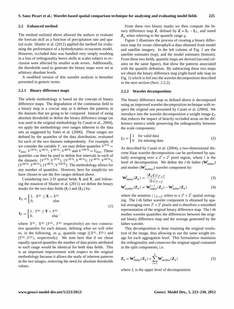
Figure1 illustrates the process of creating a binary differ-ence map for ocean chlorophyll-a data obtained from modeland satellite imagery. In the left column of Fig.1 are thesatellite estimates (top), and the model estimates (bottom).From these two fields, quantile maps are derived (second col-umn on the same figure), that show the patterns associatedwith the quantile definition. By subtracting these two mapswe obtain the binary difference map (right-hand side map onFig.1) which is fed into the wavelet decomposition describedin the next section (Sect.2.2.2).
2.2.2 Wavelet decomposition
The binary difference map as defined above is decomposedusing an improved wavelet decomposition technique with re-spect the original one presented byCasati et al.(2004). Weintroduce into the wavelet decomposition a weight imageζ 0that reduces the impact of heavily occluded areas on the dif-ference metrics while preserving the orthogonality betweenthe scale components:
ζ 0 =
{1 for valid data0 for missing data
(2)
As described byCasati et al.(2004), a two-dimensional dis-crete Haar wavelet decomposition can be performed by spa-tially averaging over a 2l × 2l pixel region, wherel is thelevel of decomposition. We define thel-th father (Wl
father)and mother (Wl
mother) wavelet component by:
Wlfather(Zq) =
〈Zqζ 0〉2l×2l
〈ζ 0〉2l×2l
(3)
Wlmother(Zq) = Wl−1
father(Zq)−Wlfather(Zq) (4)
where the notation〈·〉2l×2l refers to a 2l ×2l spatial averag-ing. Thel-th father wavelet component is obtained by spa-tial averaging over 2l ×2l pixels and is therefore a smoothedrepresentation of the original binary difference map. Thel-thmother wavelet quantifies the differences between the origi-nal binary difference map and the average generated by thefather wavelet.
This decomposition is done retaining the original resolu-tion of the image, thus allowing to use the same weight im-age for each aggregation level. This formulation maintainsthe orthogonality and conserves the original signal containedin the split components, i.e.
Zq = WLfather(Zq)+
L∑l=1
Wlmother(Zq) (5)
whereL is the upper level of decomposition.
www.geosci-model-dev.net/5/223/2012/ Geosci. Model Dev., 5, 223–230, 2012
226 S. Saux Picart et al.: Wavelet-based spatial comparison technique for analysing and evaluating model fields
Fig. 1. Binary difference map creation. On the left: re-gridded satellite (top) and model (bottom) monthly fields of surface concentration ofchlorophyll-a for May 2004. In the centre: quantile maps of the same fields (top, satellite; bottom model). On the right: binary differencemap for the uppermost quantile range.
2.2.3 Mean squared differences and skill score
For each level of decomposition (l) and each quantile (q), themean squared difference of the mother wavelet (MSEl,q ) iscomputed by:
MSEl,q =
∑[(Wl
mother(Zq)ζ 0)2]∑
ζ 0(6)
where∑
means summation over the whole domain. Theinclusion of ζ 0 allows any missing or occluded data to beaccounted for.
The overall mean squared difference is maintained throughthe decomposition and the following equation remains true:
MSEq =
L∑l=1
MSEl,q (7)
where MSEq refers to the overall mean squared difference ofthe binary difference map.
We then compute the skill score (SS) as defined inCasatiet al. (2004) which is more intuitive to interpret than theMSE: 1 means a perfect match, 0 corresponds to the com-parison of random data, below 0 represents a match worsethan due to random chance alone. The formulation of theskill score is as follow:
SSl,q = 1−MSEl,qL
2εq(1−εq)(8)
whereεq is the fraction of data contained in the quantileq.The skill score is in fact defined as the mean square errorrelative to the means square error of a random no skill simu-lation (seeCasati et al., 2004).
3 Results and discussion
In this section we demonstrate how the wavelet analysis canbe used to interpret the differences between model and satel-lite fields. The methodology is applied to study the case ofchlorophyll-a and SST in the North East Atlantic Europeanshelf sea.
Geosci. Model Dev., 5, 223–230, 2012 www.geosci-model-dev.net/5/223/2012/
S. Saux Picart et al.: Wavelet-based spatial comparison technique for analysing and evaluating model fields 227
3.1 Satellite data and hydrodynamic-ecosystem model
To accommodate the reader we give brief introductions tothe data sets used in the examples. We shall not go into thedetails of the geophysical application and the implications ofthe skill assessment, but rather provide a quick overview toenable the reader to fully understand the methodology andits benefits. The data shown serve simply as examples toprovide a show case for the methodology.
The model used in this work is an implementation of thePOLCOMS-ERSEM model (Allen et al., 2001, 2007) for thedynamics of the lower trophic level of the marine ecosys-tem. It provides full four-dimensional data for hydrody-namic, organic and inorganic states of the marine ecosystemat a horizontal resolution of roughly 12 km and at tempo-ral scales of 15 min. In particular it provides fields for aver-age chlorophyll-aconcentration and sea-surface temperature,which were used in this study.
To evaluate these model data, two satellite datasets wereused:
– Globcolour chlorophyll-a global dataset. This datasetconsists of daily chlorophyll-a estimates at a spatialresolution of∼4 km (based on data from three opticalwavelength satellite sensors).
– Pathfinder sea surface temperature (SST) global dataset.This dataset consists of daily sea surface temperatureestimates at a spatial resolution of∼4 km (based on datafrom a thermal infrared satellite sensor).
For a fair comparison, the region of interest (which is themodel domain) is first extracted from the satellite globaldataset. The extracted satellite data are then re-gridded tothe coarser model grid using a bilinear interpolation.
As suggested byShutler et al.(2011) we compute the op-tical depth averaged chlorophyll-a concentration to comparewith satellite estimates of chlorophyll-a which are represen-tative of a variable depth depending on the constituent in thewater. The model outputs are then cloud-masked on a dailybasis using the contemporaneous satellite masks. Finally,monthly composites are created by averaging daily modeland satellite data.
We then analyse all data for 2003–2004. The analysis pre-sented hereafter is based on the definition of five quantileranges as described in Sect.2.2.1. Each quantile range there-fore holds 20 % of the distribution and in Eq. (8) we alwayshaveεq = 0.2.
3.2 Spatio/temporal evaluation of the North EastEuropean shelf sea modelling
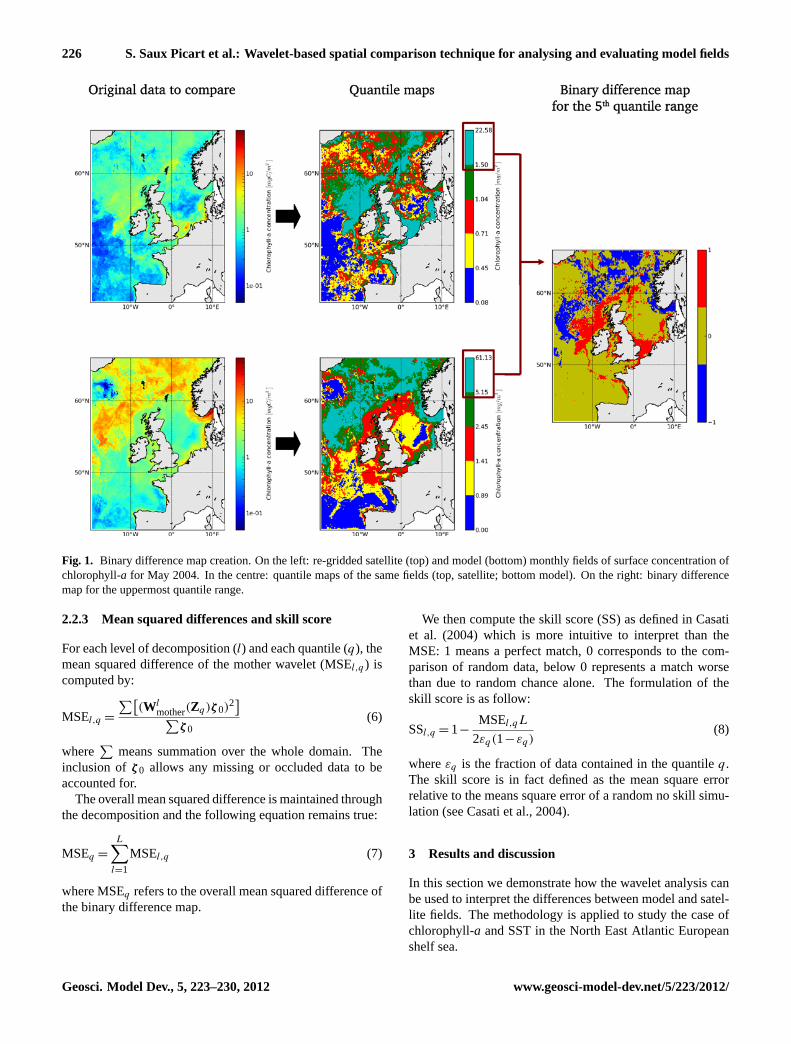
Figure 2 shows an example application of the methodol-ogy for fields of sea surface temperature (Fig.2a) andchlorophyll-a concentration (Fig.2b). Quantiles are reportedon the x-axis with the corresponding lower and upper values
Discu
ssionPaper
|Discu
ssionPaper
|Discu
ssionPaper
|Discu
ssionPaper
|
(a)
(b)
Fig. 2: Spatial scales versus quantile ranges plots for May 2004. Sea surface temper-ature (a) and chlorophyll-a concentration (b) skill scores.
20
Fig. 2. Spatial scales versus quantile rangesplots for May 2004.Sea surface temperature(a) and chlorophyll-a concentration(b)skill scores.
for the satellite and model data. The y-axis shows the spatialscale in kilometres (km).
The methodology highlights scales and ranges of skill.One can notice a lower skill score at small scales (24 km) forboth SST and chlorophyll-a for almost all ranges. One canalso note higher model skills for the lowest and the highestquantiles at all spatial scales for SST.
This is less true for chlorophyll-a, where a low model skillis observed at high spatial scale (of about∼700 km) for thelast quantile (high value of chlorophyll-a). This can be con-firmed by looking at the corresponding binary difference map(right-hand map on Fig.1) where large scale differences areclearly visible in the north of the domain. An interpretationfor that observation is a spatial mismatch (or misplacement)of a large summer bloom of chlorophyll-a in the north of thedomain.
This methodology also allows us to perform inter-comparison of results for different variables and differenttimes (providing they refer to the same geophysical domain).
www.geosci-model-dev.net/5/223/2012/ Geosci. Model Dev., 5, 223–230, 2012
228 S. Saux Picart et al.: Wavelet-based spatial comparison technique for analysing and evaluating model fieldsDiscu
ssionPaper
|Discu
ssionPaper
|Discu
ssionPaper
|Discu
ssionPaper
|
(a)
(b)
Fig. 3: Spatial scales versus time plot for the 5th quantile (80-100%) 2003-2004. Seasurface temperature (a) and chlorophyll-a concentration (b) skill scores.
21
Fig. 3. Spatial scales versus timeplot for the 5th quantile (80–100 %) 2003–2004. Sea surface temperature(a) and chlorophyll-aconcentration(b) skill scores.
Figure3 shows a time/space skill score plot. Time has beenreported on thex axis and spatial scale on they axis, theshades of grey represent the skill score of the wavelet decom-position for the 5th quantile. The 5th quantile corresponds tothe upper range of sea surface temperature and chlorophyll-a, which in our example can be interpreted as extreme events(i.e. an algal bloom or a temperature anomaly).
Figure3a shows that sea surface temperature skill scorehas high values throughout the year at all spatial scales forthe 5th quantile. A small region of slightly lower skill scorecan be observed during January–March at spatial scales ofabout 200–400 km. We can also note a slightly lower skillscore at low spatial scale throughout the year.
The chlorophyll-a skill score (shown on Fig.3b) is gener-ally lower than the one of temperature and shows some inter-esting features. As for the sea surface temperature, we canobserve a poorer skill score at low scale (first level of aggre-gation) throughout the year. However we can additionallyobserve a consistent patch of low skill in June–August be-tween 100 and 800 km. This pattern does not appear on thetemperature skill score.
3.3 Interpretation of the skill score in terms of modelevaluation
Low skill scores observed at small spatial scales (∼24 km) inboth chlorophyll-a and SST model output can be explainedby the high small scale variability in the satellite data thatis not reproduced by the model. It is indeed easier to cap-ture low frequency variations and trends. Ocean colour andinfrared remote sensing are strongly impacted by varioussources of uncertainties including measurement noise, cali-bration noise or atmospheric correction uncertainties. How-ever, these results also illustrate the complexity of modellingbiological systems.
The generally higher skill scores obtained for SST, atall scales and for all quantile ranges, (compared withchlorophyll-a) highlight the strength of the hydrodynamicmodel fed with high quality surface forcing and boundaryconditions (Siddorn et al., 2007). One should also note thatchlorophyll-a estimates from ocean colour data are represen-tative of a variable and unknown depth: the water leaving ra-diances (used to derive chlorophyll-a concentration) includecontributions from the surface to a finite depth which varieswith the optical properties of the water. For that reason, wechoose to average the model chlorophyll-a over the opticaldepth (of the model), but an uncertainty still remains.
Finally, the consistent appearance of low skill scores inchlorophyll-a (5th quantile) analysis during June–August atlarge scale is correlated with the summer algal bloom offScotland and Ireland coast. On the satellite chlorophyll-afield provided on the top-left map of Fig.1, one can see highchlorophyll-a values (2–8 mg m−3) along the northwest coastof Scotland and Ireland, whereas in the model field, the high-est chlorophyll-a values are observed further in the northwestdirection and extend further toward the northwest coast ofNorway. This translates into the large scale misplacement ofpattern visible on the binary difference map (right map onFig. 1).
3.4 Discussion
When comparing model output to another dataset, one mayobserve differences in the characteristics and possibly in theshape of data distributions. However, the model can stillshow some skill in representing relative patterns such as ex-treme events for example. It is therefore important to use amethodology which will be able to highlight the skill of themodel without being affected by the bias or the data distribu-tion shape. The bias can be studied separately using simpleclassical methods but it is worth noting that one can comparethe size and mean value of quantile ranges to study it in moredetail (for each quantile range separately).
The method presented here allows the comparison of in-herent spatial structures within two data sets at differentscales. This process is not affected by the overall bias or re-spective dispersion of the data, as was the case in the original
Geosci. Model Dev., 5, 223–230, 2012 www.geosci-model-dev.net/5/223/2012/
S. Saux Picart et al.: Wavelet-based spatial comparison technique for analysing and evaluating model fields 229
Discu
ssionPaper
|Discu
ssionPaper
|Discu
ssionPaper
|Discu
ssionPaper
|
Fig. 4: Illustration of the effect of a bias on the binary masks as defined in section2.2.1. a and b are two sample data array where b displays a bias with respect to a.c and d are the binary masks obtained considering an absolute threshold that is theoverall mean value of a and b. e and f are the binary masks obtained using the quantileapproach introduced in section 2.2.1.
22
Fig. 4. Illustration of the effect of a bias on the binary masks asdefined in Sect.2.2.1. (a) and(b) are two sample data array where(b) displays a bias with respect to(a). (c) and (d) are the binarymasks obtained considering an absolute threshold that is the overallmean value of(a) and(b). (e)and(f) are the binary masks obtainedusing the quantile approach introduced in Sect.2.2.1.
version when using absolute thresholds. This is illustratedby Figs.4 and5. Starting from two 2-D data arrays that haveexactly the same patterns but a systematic difference (bias),Fig. 4c and d illustrates how using absolute thresholds leadsto completely different binary masks. However, using rela-tive thresholds (quantiles) enables the comparison of inherentspatial structures of the data sets (Fig.4e and f).
Moreover, if we consider two data sets with the same pat-terns but different distributions (Fig.5a–d), the binary masksdefined by absolute thresholds are very different (Fig.5e andf) and do not represent comparable structures. The use ofquantile definitions provides a more robust definition of thepatterns (Fig.5e and f).
From the two illustrative examples described above, it isclear that if one would use absolute thresholds as break-offcriteria for the binary maps, qualitatively similar patternsmay appear to be structurally different. An additional benefitof the quantile definition is that it yields the same amount ofdata points in each quantile range hence guarantees equiva-lent structural maps.
The wavelet decomposition we described in Sect.2.2.2also provides more confidence to the results especially atthe higher aggregation levels when comparing data sets withgaps. Applying the original method ofCasati et al.(2004)to masked data, a cell (at high aggregation level) that con-tains very few valid values and a cell containing only validvalues would have had the same impact on the overall MSE.The introduction of the weight imageζ 0 is a mathematicalsolution that gives appropriate impact factors to each cell inrelation to the data gap contained within it, while preserv-ing the fundamental characteristics of the decomposition, i.e.the orthogonality between the wavelet components and theconservation of the original signal (Eq.5).
Discu
ssionPaper
|Discu
ssionPaper
|Discu
ssionPaper
|Discu
ssionPaper
|
Fig. 5: Illustration of the effect of differences in distributions in the two datasets. aand b are two sample data arrays where b is a power function of a. c and d are theirrespective histograms. e and f are the binary masks obtained considering an absolutethreshold that is the overall mean value of a and b. g and h are the binary masksobtained using the quantile approach introduced in section 2.2.1, i.e. the median inthis case
23
Fig. 5. Illustration of the effect of differences in distributions in thetwo datasets.(a) and(b) are two sample data arrays where(b) is apower function of(a). (c) and(d) are their respective histograms.(e) and (f) are the binary masks obtained considering an absolutethreshold that is the overall mean value of(a) and(b). (g) and(h)are the binary masks obtained using the quantile approach intro-duced in Sect.2.2.1, i.e. the median in this case.
This methodology is based on statistically robust metricsand the choice of the threshold is driven by the data distribu-tion, and hence is more objective (for example this allows thestudy of patterns of extreme events of chlorophyll-a) in com-paring the inherent structures of the datasets. This is partic-ularly useful for temporal intercomparisons ie for situationswhere the bias in different time series is potentially different.
4 Conclusions
The approach presented here has been developed to comparethe spatial structures in two datasets. It allows any spatialdifferences to be decomposed into their orthogonal compo-nents. The method is composed of two steps: (i) definition ofbinary error map based on quantile classification (ii) waveletdecomposition of the binary error map and computation ofa skill score for each level of decomposition. The approachis generic in the sense that it requires no tuning or parame-ter selection as thresholding to generate the binary differencemaps is determined based on the statistical distribution of theinput datasets. Furthermore, the approach is able to handledata containing biases or occluded (missing) data, withoutloss of orthogonality. We have demonstrated its applicationby analysing a series of scenes of model output with opti-cal wavelength satellite data. The methodology provides theability to identify the spatial scales of the features that themodel is able to reproduce focusing on the inherent structuresof the datasets independently of bias or normalised standarddeviation.
www.geosci-model-dev.net/5/223/2012/ Geosci. Model Dev., 5, 223–230, 2012
230 S. Saux Picart et al.: Wavelet-based spatial comparison technique for analysing and evaluating model fields
The results can be visualised in two very synthetic ways: aspatial scales versus quantile rangesplot, which can be usedto identify the overall match/mismatch of the features in two2-D data fields; and aspatial scales versus timeplot, whichcan be used to analyse extreme events. Alternatively, if oneis interested in a specific spatial scale, a time/quantile plotwould provide useful information over the whole data range.
This methodology, used in combination with other classi-cal ways of comparing two datasets, is a powerful evaluationtool (when comparing Earth observation data and model out-put) because it is objective and independent of the datasetdistribution. It is therefore a very useful tool that can serveto justify or guide the choice of a model for a specific ap-plication. In the context of marine hydrological/ecosystemmodelling these can be carbon budget, harmful algal bloomdetection, ecosystem management.
One can also use this methodology as a way of comparingoutputs from two different model. The method provides asynthetic way of representing the spatial effect of two differ-ent parametrisations, or the effect of using different boundaryconditions or forcing data in terms of spatial features.
Future work will concentrate on extending the approach toinclude the time dimension. This would enable a completepicture of the model skill to be considered including sea-sonal forecasts and the study of inter-annual or multi-decadaltrends.
Supplementary material related to thisarticle is available online at:http://www.geosci-model-dev.net/5/223/2012/gmd-5-223-2012-supplement.zip.
Acknowledgements.The authors would like to thank MyOceanproject for supplying Globcolour data for this study. TheAVHRR Oceans Pathfinder SST data were obtained from thePhysical Oceanography Distributed Active Archive Center(PO.DAAC) at the NASA Jet Propulsion Laboratory, Pasadena,CA. http://podaac.jpl.nasa.gov. The authors thank the NERC EarthObservation Data Acquisition and Analysis Service (NEODAAS)for providing computing facilities and data storage. This work wasfunded by the UK NERC Oceans 2025 program theme 9, NextGeneration Ecosystem Models. This work was partially supportedby the EC FP7 MyOcean research and development project“Improving CO2 Flux Estimations from the MyOcean Atlanticnorth west shelf hydrodynamic ecosystem model (IFEMA)”.
Edited by: J. Annan
References
Allen, J. I., Blackford, J. C., Holt, J. T., Proctor, R., Ashworth, M.,and Siddorn, J. R.: A highly spatially resolved ecosystem modelfor the North West European Continental Shelf, Sarsia, 86, 423–440, 2001.
Allen, J. I., Somerfield, P., and Gilbert, F.: Quantifying uncertaintyin high-resolution coupled hydrodynamic-ecosystem models,J. Marine Syst., 64, 3–14,doi:10.1016/j.jmarsys.2006.02.010,2007.
Bougeault, P.: The WGNE survey of verification methods fornumerical prediction of weather elements and severe weatherevents, Tech. rep., Technical report, WMO, 2003.
Briggs, W. M. and Levine, R. A.: Wavelets and field forecast verifi-cation, B. Am. Meteor. Soc., 125, 1329–1341, 1997.
Casati, B.: New Developments of the Intensity-Scale Tech-nique within the Spatial Verification Methods Inter-comparison Project, Weather Forecast., 25, 113–143,doi:10.1175/2009WAF2222257.1, 2010.
Casati, B., Ross, G., and Stephenson, D.: A new intensity-scale ap-proach for the verification of spatial precipitation forecasts, Me-teorol. Appl., 11, 141–154, 2004.
Doney, S. C., Lima, I., Moore, J. K., Lindsay, K., Behrenfeld, M. J.,Westberry, T. K., Mahowald, N., Glover, D. M., and Takahashi,T.: Skill metrics for confronting global upper ocean ecosystem-biogeochemistry models against field and remote sensing data, J.Marine Syst., 76, 95–112, 2009.
Ebert, E. E., Damrath, U., Wergen, W., and Baldwin, E.: TheWGNE assessment of short-term quantitative precipitation fore-casts (QPFs) from operational numerical weather predictionmodels, B. Am. Meteor. Soc., 84, 481–492, 2003.
Haar, A.: Zur Theorie der orthogonalen Funktionensysteme, Math.Ann., 69, 331–371, 1910 (in German).
Jones, A., Thomson, D., Hort, M., and Devenish, B.: The UKMet Office’s Next-Generation Atmospheric Dispersion Model,NAME III, NATO Challenges of Modern Series, 580–589, 2007.
Lehr, W., Wesley, D., Simecek-Beatty, D., Jones, R., Kachook, G.,and Lankford, J.: Algorithm and interface modifications of theNOAA oil spill behavior model, in: Proceedings of the Twenty-Third Arctic and Marine Oilspill Program (AMOP) TechnicalSeminar, 525–540, 2000.
Shutler, J., Smyth, T., Saux Picart, S., Wakelin, S., Hyder, P.,Grant, M., Orekhov, P., Tilstone, G., and Allen, J. I.: Evalu-ating the ability of a hydrodynamic ecosystem model to cap-ture inter- and intra-annual spatial characteristics of chlorophyll-a in the north east Atlantic, J. Marine Syst., 88, 169–182,doi:10.1016/j.jmarsys.2011.03.013, 2011.
Siddorn, J. R., Allen, J. I., Blackford, J. C., Gilbert, F. J., Holt, J. T.,Hort, M. W., Osborne, J. P., Proctor, R., and Mills, D. K.: Mod-elling the hydrodynamics and ecosystem of the North-West Eu-ropean continental shelf for operational oceanography, J. MarineSyst., 65, 417–429,doi:10.1016/j.jmarsys.2006.01.018, 2007.
Stow, C. A., Jolliff, J., McGillicuddy Jr., D. J., Doney, S. C., Allen,J. I., Friedrichs, M. A., Rose, K. A., and Wallhead, P.: Skill as-sessment for coupled biological/physical models of marine sys-tems, J. Marine Syst., 76, 4–15, 2009.
Tiedje, B., Moll, A., and Kaleschke, L.: Comparison of temporaland spatial structures of chlorophyll derived from MODIS satel-lite data and ECOHAM3 model data in the North Sea, J. SeaRes., 64, 250–259, 2010.
Yates, E., Anquetin, S., Ducrocq, V., Creutin, J.-D., Ri-card, D., and Chancibault, K.: Point and areal validationof forecast precipitation fields, Meteorol. Appl., 13, 1–20,doi:10.1017/S1350482705001921, 2006.
Geosci. Model Dev., 5, 223–230, 2012 www.geosci-model-dev.net/5/223/2012/