(Weak) Gravitational lensing(A review)

Martin WhiteUC Berkeley

GGI 2006

Overview• Cosmic shear is the distortion of the shapes of

background galaxies due to the bending of light bythe potentials associated with large-scale structure.

• For sources at zs~1 and structure at 0.1<z<1 it is apercent level effect which can only be detectedstatistically.

• Theoretically clean.• Observationally tractable.

http://mwhite.berkeley.edu/Lensing/

Outline• Basic lensing theory• Describing spin-2 fields• Measuring shear• Shear statistics• Tomography & inversion• Current status of observations• Future plans• Weak lensing and dark energy• Simulating weak lensing• Lensing the CMB

Lensing basicsRecall that photons travel along null geodesics. We can solvefor the photon path by extremizing the Lagrangian for force freemotion

This leads to the following Euler-Lagrange equations:

For the weak field metric

Lensing basics (contd)We obtain to first order in Φ:

which integrates immediately to (becoming cosmological now)

The change in position on a plane perpendicular to the line-of-sight is

Integrating and dividing by r(χ) yields the mapping

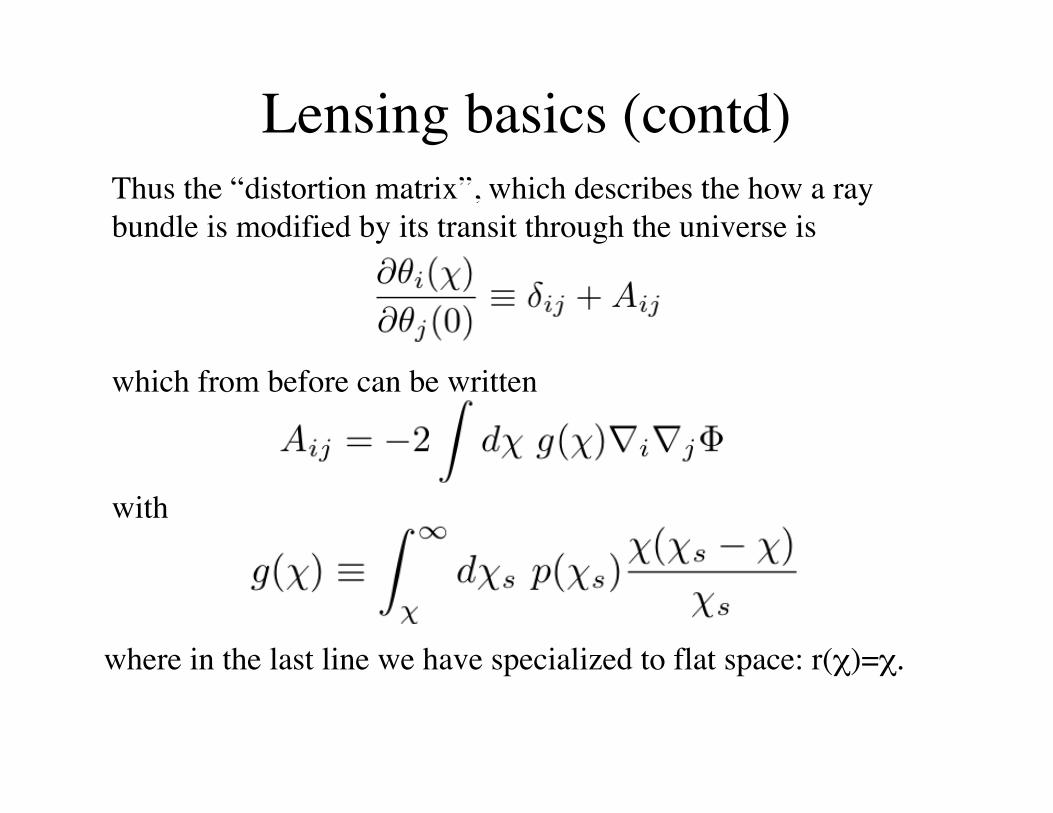
Lensing basics (contd)Thus the “distortion matrix”, which describes the how a raybundle is modified by its transit through the universe is

which from before can be written

with

where in the last line we have specialized to flat space: r(χ)=χ.

Lensing weightLensing is most efficient for structure mid-way between the

observer and the source.

Lensing basics (contd)The distortion matrix A is conventionally decomposed as

If the size of the image is not known a priori then κ cannot bemeasured directly. Taking a factor of (1-κ) out front of 1+Awe find we can only measure the reduced shear g=γ/(1-κ).

γ1>0 γ1<0 γ2>0 γ2<0

where κ<<1 is the convergence and γ<<1 is the shear.The rotation, ω, only comes from higher order effects and ismuch smaller than κ or γ.

Lensing basics (contd)The integral defining A should be taken along the perturbedphoton path, but the deflection is typically small, so to 1st orderwe can integrate along a straight line (Born approximation).

Then A is the second derivative of a projected potential:

Since κ and γ come from a single potential, φ, they can berelated via

(Kaiser-Squires “method” -- note non-local)

Lensing basics (contd)If we relate the potential to the density by Poisson’s equation,integrate by parts and ignore the surface term

In the Born limit, the convergence is (almost) the projected mass.

It is straightforward to show that a positive, radially symmetricκ leads to a tangential shear:

A simulated shear field

2 degrees

Obvious non-linearstructure, with sheartangential about κ peaks oftypical size ~1 arcmin.

Filamentary structure erasedby projection.

Shear field sampled(regularly) at about the levelachievable observationallyfrom deep space based data.

Spin-2 fieldsThe shearing of images is a spin-2 field. It is useful to spendsome time on the description of spin-2 fields.

Rotating the coordinate system counterclockwise by φ changes

Under a rotation by π the field is left unchanged.A rotation by π/2 changes γ1 to γ2 and γ2 to -γ1.

γ1>0 γ1<0 γ2>0 γ2<0

Spin-2 fields (contd)Keeping track of that phase as we rotate coordinates, the Fourierdecomposition can be written in terms of real functions ε and β as

where ε is parity even and β is parity odd.

The E-mode is simply κ -- tangential sheararound overdensities.

The B-mode is very small for gravitationallensing -- “swirling” around overdensities.

Spin-2 fields (contd)In the full-sky limit the Fourier transforms become sphericalharmonic transforms and Bessel functions become Wignerfunctions … we gain little by the more general treatment here.For our purposes k = l!

For any given line joining two points it is useful to define γ+ andγx wrt the implied axes as

where γ+ is the tangential shear.

2-point functionsIf the field is translationally invariant, the Fourier description isuseful since <εε> etc are diagonal in k or l.

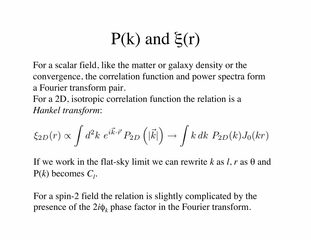
P(k) and ξ(r)For a scalar field, like the matter or galaxy density or theconvergence, the correlation function and power spectra forma Fourier transform pair.For a 2D, isotropic correlation function the relation is aHankel transform:

If we work in the flat-sky limit we can rewrite k as l, r as θ andP(k) becomes Cl.

For a spin-2 field the relation is slightly complicated by thepresence of the 2iφk phase factor in the Fourier transform.

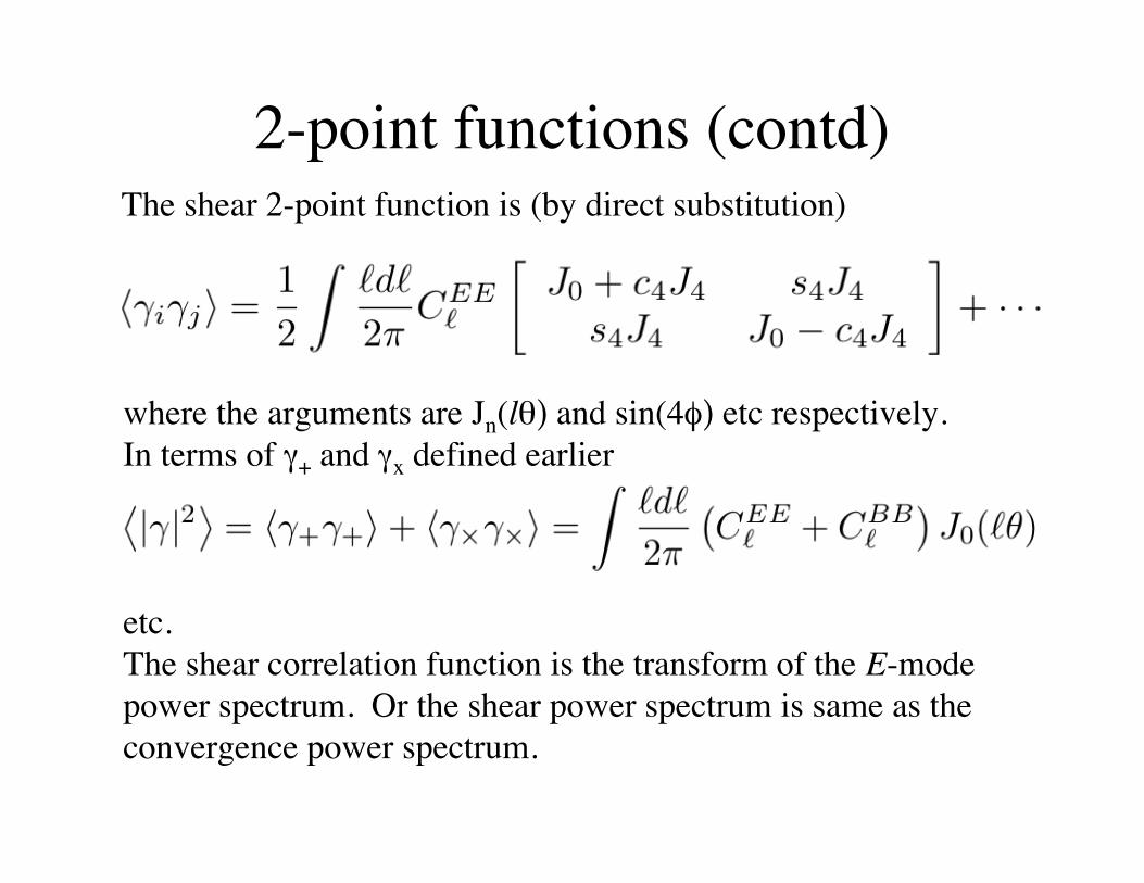
2-point functions (contd)The shear 2-point function is (by direct substitution)

where the arguments are Jn(lθ) and sin(4φ) etc respectively.In terms of γ+ and γx defined earlier

etc.The shear correlation function is the transform of the E-modepower spectrum. Or the shear power spectrum is same as theconvergence power spectrum.

2-point functions (contd)• All other 2-point functions can be written in terms of

integrals of the power spectrum times window functions,e.g. shear variance

• Conversion from one quantity to another may not be asstraightforward as it could be due to limited range ofobservations.

Limber approximationThe Limber approximation allows us tocompute the statistics of any projected quantityas an integral over the statistics of the 3Dquantity. In its simplest form

The physical content of the Limber approximationis that, for sufficiently broad w, only k3=0 survivesand a given angular scales receives contributionsfrom transverse modes.

2λ

kχ=l

Lensing power spectrumLensing is an obvious candidate for the Limber approximation

The lensing power spectrum issensitive to the distance factors,the matter density and the growthof large-scale structure.

Over most of the measurablerange it is dominated by non-linear gravitational clustering.

Projection geometry

2λ

kχ=l

Aperture massIt is often useful to work with a scalar quantity which isderivable from the shear, is reasonably local and allows a simpleE/B decomposition. The “aperture mass” is such a quantity.Starting from the relation between κ and γ one can show

for any compact, compensated filter U where

Map has a scale beyond which U vanishes.Map probes only E-modes (replacing γ+ with γx gives B-mode)

Aperture mass (contd)

Advantages:• Map can be calculated directly from γ without the

need for mass reconstruction.• Generally Map is compact in both real and Fourier

space (e.g. the kernel for Var[Map] is J4)• Map decorrelates rapidly beyond the filter scale, so

most information is in variance, skewness etc.

If we pick U to look like a cluster profile, then Map willbe akin to a matched filter.

Generally it is a bandpass filter applied to the κ map.

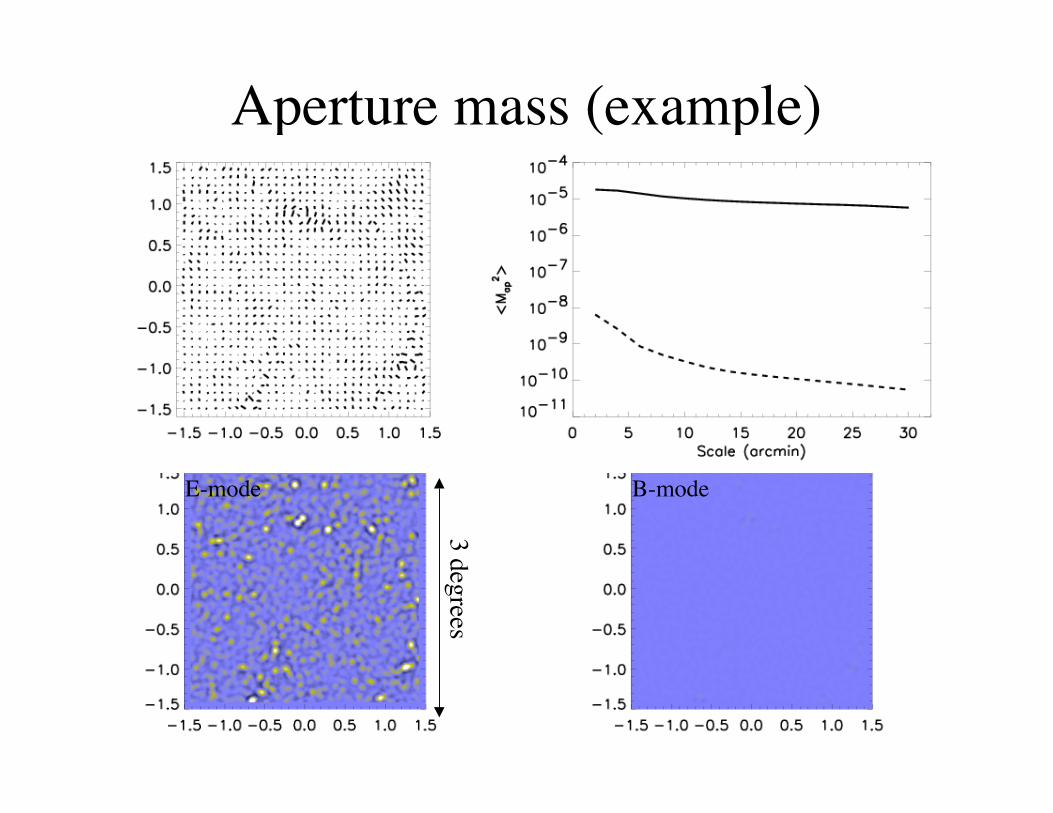
Aperture mass (example)

E-mode B-mode

3 degrees

Measuring ShearSince we don’t know a priori the positions of galaxies, thedeflection is not measurable. However the shearing of shapesor (potentially) the change in sky area is. [Flexion]

Thus we need to work with information about galaxy shapes.The simplest information is the (weighted) moment of inertia:

Under Aij the moment of inertia transforms as

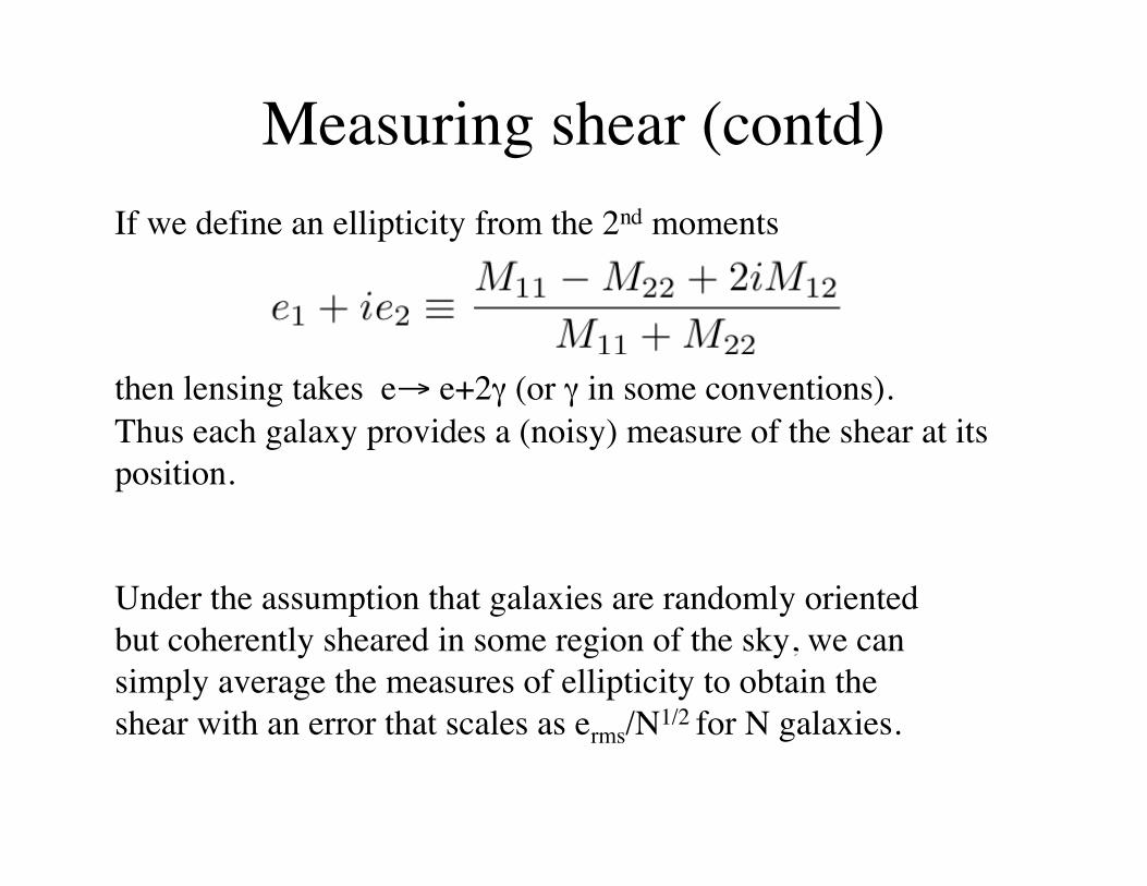
Measuring shear (contd)If we define an ellipticity from the 2nd moments

then lensing takes e→ e+2γ (or γ in some conventions).Thus each galaxy provides a (noisy) measure of the shear at itsposition.

Under the assumption that galaxies are randomly orientedbut coherently sheared in some region of the sky, we cansimply average the measures of ellipticity to obtain theshear with an error that scales as erms/N1/2 for N galaxies.

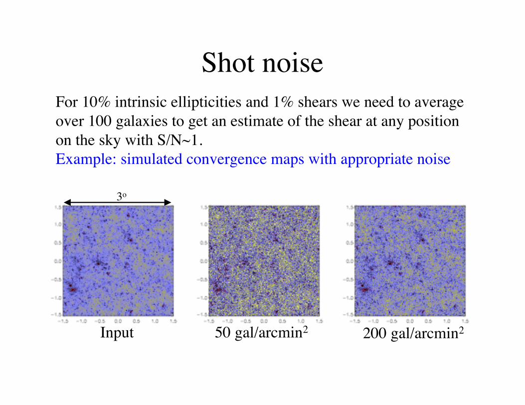
Shot noiseFor 10% intrinsic ellipticities and 1% shears we need to averageover 100 galaxies to get an estimate of the shear at any positionon the sky with S/N~1.Example: simulated convergence maps with appropriate noise

Input

3o

50 gal/arcmin2 200 gal/arcmin2

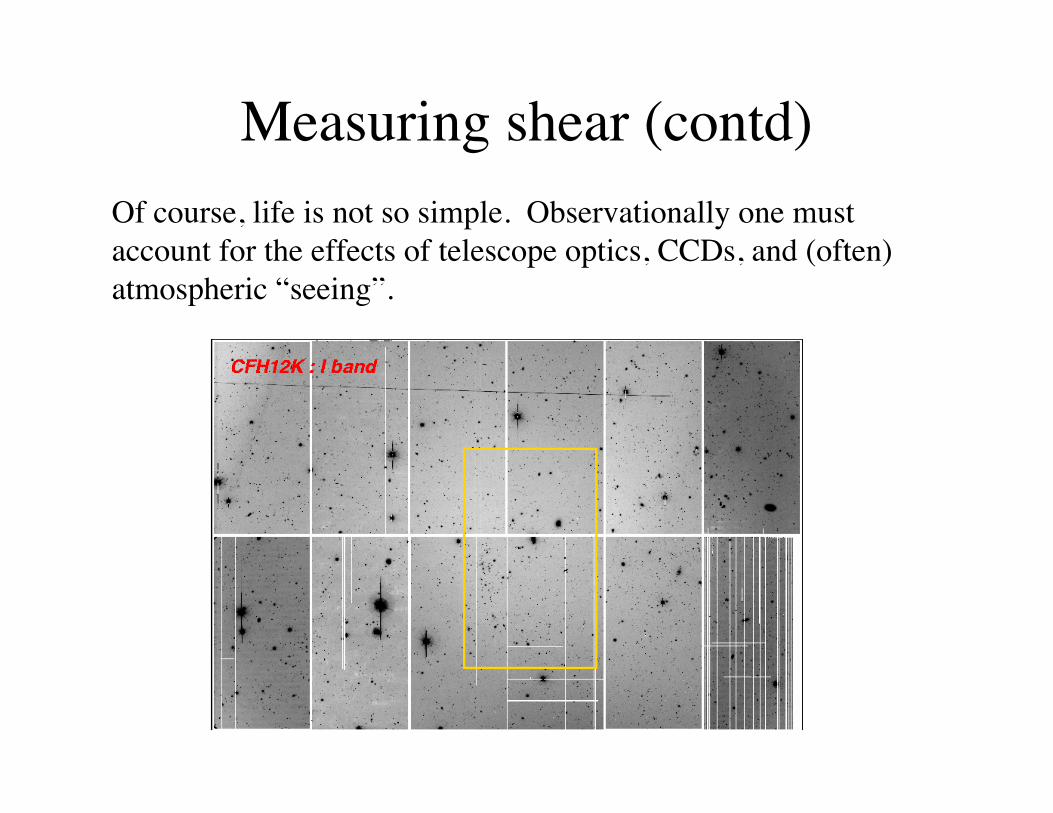
Measuring shear (contd)Of course, life is not so simple. Observationally one mustaccount for the effects of telescope optics, CCDs, and (often)atmospheric “seeing”.

PSF anisotropy

3-10% rms reduced to ≈0.1%

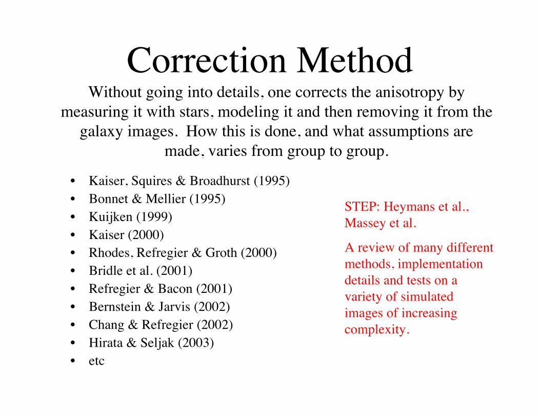
Correction MethodWithout going into details, one corrects the anisotropy by

measuring it with stars, modeling it and then removing it from thegalaxy images. How this is done, and what assumptions are

made, varies from group to group.

• Kaiser, Squires & Broadhurst (1995)• Bonnet & Mellier (1995)• Kuijken (1999)• Kaiser (2000)• Rhodes, Refregier & Groth (2000)• Bridle et al. (2001)• Refregier & Bacon (2001)• Bernstein & Jarvis (2002)• Chang & Refregier (2002)• Hirata & Seljak (2003)• etc

STEP: Heymans et al.,Massey et al.

A review of many differentmethods, implementationdetails and tests on avariety of simulatedimages of increasingcomplexity.

Correction method (details)Corrections for seeing, PSF etc. all follow a similar derivation:We take the “true” image and convolve it with some distortion(shear, smear, optics, seeing, …).How does this affect the measured ellipticities?

Convolving I(θ) with g implies:

where

Integrating Z by parts and writing the elements of qlm as qβ we have

KSB’95Original method:

PSF Anisotropy:

PSF Smear & Shear Calibration: gP εγ γ 1)( −=

Need to extrapolate from measured stellar positions to observedgalaxy positions. Modeling this “well” is key, new techniques using

PCA (Jain et al. 2005) offer hope that this will improve as datavolume improves - allowing N-1/2 scaling!

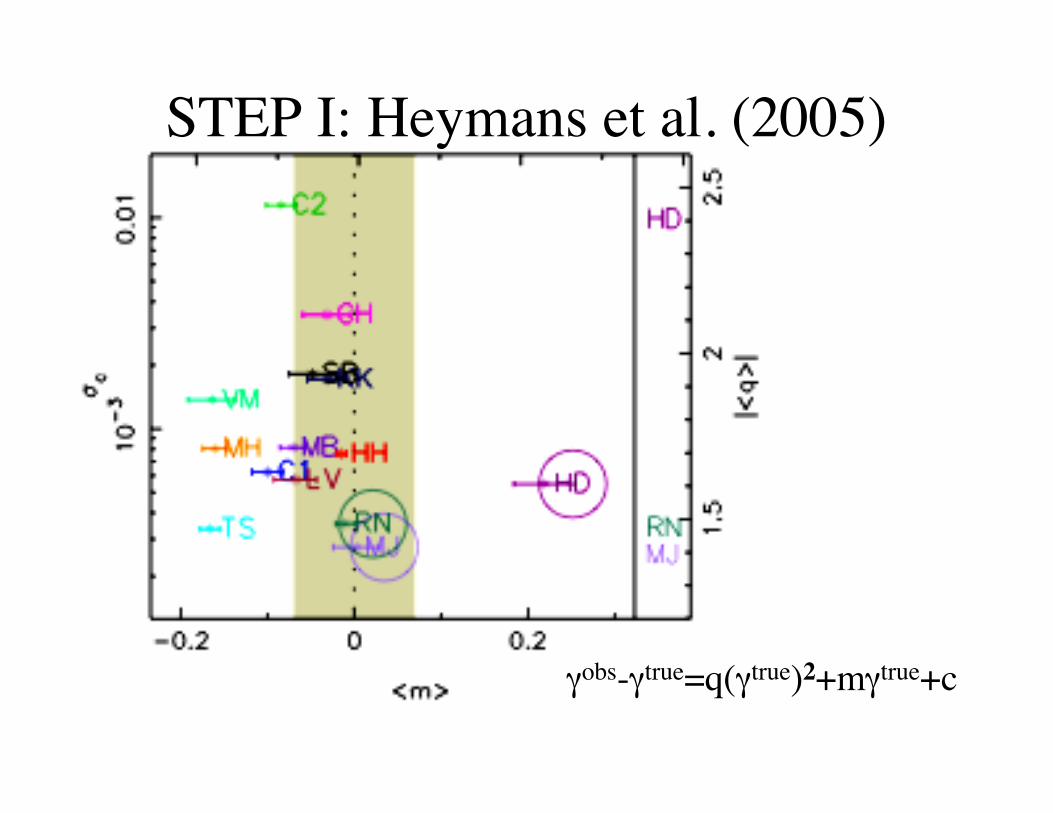
STEP I: Heymans et al. (2005)

γobs-γtrue=q(γtrue)2+mγtrue+c

Intrinsic alignmentsWe must also worry about intrinsic alignments of galaxies which wouldviolate our “random orientation” hypothesis.

Theoretically we expect such alignments to drop rapidly as the separation ofthe galaxy pairs is increased which allows us to mitigate the problemobservationally (see later).

By measuring the “shear” of nearby samples, where lensing is small, wecan estimate the size of the intrinsic alignment effect.It is small!

In principle it is even possible that we will need to worry about correlationsin the alignment of a background galaxy with foreground mass which canlens-especially if we wish to do tomography(Hirata & Seljak 2004, Mandelbaum et al. 2006, Heymans et al. 2006).

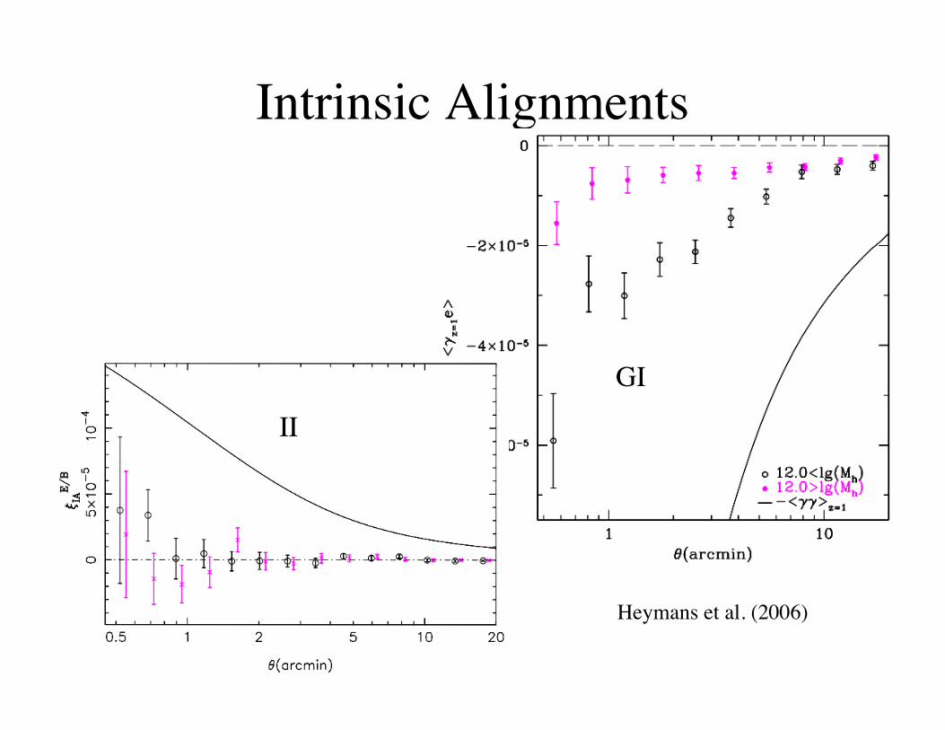
Intrinsic Alignments

II

GI

Heymans et al. (2006)

Correlation function(s)Given a series of measures of “shear” for galaxies i, constructestimators of e.g. the correlation function

Measure γ1 in the coordinatesystem aligned with theseparation vector.

Transform gives the powerspectrum (plus shot noise).

Shear statistics• Shear variance in cells of size θ

– Easy to measure– Highly correlated

• Power spectra– Easy to interpret theoretically– Hard to measure with high dynamic range and gappy

data.• Correlation function(s)

– Handles complex geometries well– Correlated errors

• Map variances on scale θ– Produces a scalar from γ field & good E/B separation– Mixes scales, and systematics

Measuring the power spectrumTheorists usally work in terms of the power spectrum Cl.For a Gaussian field measured over fsky of the sky with a finitenumber of galaxies the error is:

fsky = 10%

fsky = 100%

(Δl=0.1l)

ngal=100, 50, 25/arcmin2

fsky = 1%

• Shear 3-point correlation function(s)

• Higher moments of Map

• Counts of peaks in Map or κ from γ field

Higher order statisticsLensing is clearly non-Gaussian, so there is more to life than the2-point function. In fact Takada & Jain have shown that there isas much information* in the 3-point function as the 2-point fn.

Line from COM to vertexdefines axes for γ+ and γx

(Best description not yet known …)

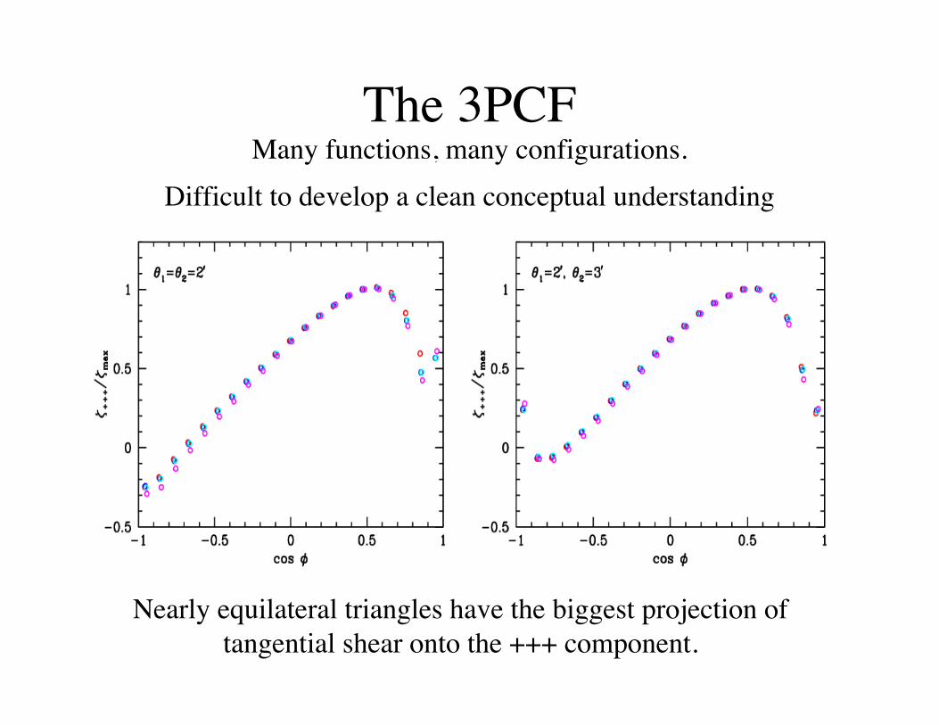
The 3PCFMany functions, many configurations.

Difficult to develop a clean conceptual understanding

Nearly equilateral triangles have the biggest projection oftangential shear onto the +++ component.

The halo model• “Traditional” methods for treating trans- or non-

linear power (e.g. PT, HEPT, etc) don’t work verywell for lensing. Need a new approach.

• Halo model– For estimating the shape of the 3-point function, the

errors on cosmological parameters or correlationsbetween Cl bins one can use the “halo model”.

– The calculations can be quite simple: e.g. on the scalesof relevance the 4-point function, for δCl, is dominatedby the 1-halo term (Cooray et al.).

– This model borrows heavily from simulations and ismore of a “guide” than a precise calculational tool, butis currently sufficient.

Tomography and cosmography

Adding source redshift information

Adding the third dimension

• One of the main limitations of lensing isthat it is inherently a projected signal.

• Signal builds up over Gpc along los.• However if we have source redshift

information (spectroscopic or photometric)we can try to break things into slices andregain (some of) the 3rd dimension.

Tomography• Tomography refers

to the use ofinformation frommultiple sourceredshifts.

• This adds some“depth” informationto lensing --important forevolution studies.

Takada …

Tomography (contd)

If we divide the sourcesinto bins labelled by a, bthen we promote Cl toCl

(ab), etc.

Since g(χ) is so broad,different source bins arevery correlated (r>0.9).Gains saturate quickly!

If ignore a=b, then remove almostall intrinsic alignment with littleloss of cosmological informationfor N>3 bins. (Takada & White)

The generalization is straightforward for any statistic.

z1 z2

Taylor inversion formula• As an aside, Andy Taylor has shown that there is

an exact inversion of the lensing kernel for theprojected potential:

• has inverse

• Practical uses of this formula have not really beenfound.

C(ross) C(orrelation) C(osmography)

• Imagine a single object lensing two sourcesat z1 and z2. For a thin lens of mass Σl

where the weights depend only on distanceratios for objects of known redshift.

• Taking the ratio of κ’s gives a distance ratioof ratios as a function of z, independent ofstructure!

(Jain & Taylor, Bernstein & Jain, Hu & Jain)

CCC (contd)• In principle very clean, but the distance ratio of ratios

change only slowly with cosmology, e.g. w.• Need to understand source redshift distribution extremely

well:– Redshift systematics need to be smaller than 0.1% in ln[1+z]!

• Actual implementation is in terms of cross-correlation offoreground and background shears and galaxies.

• Forecasted performance is unclear, as it depends ondiffering assumptions.

Offset-linear scaling(Zhang, Hui & Stebbins 2005)

If Wb and Wf don’t overlap can drop first Θ function and the χbdependence simplifies to:

By measuring Pκ for different zb can isolate χ(z)!Like CCC this method is elegant and clean, but not aspowerful as using the non-geometric information as well.

ObservationsFirst detections of cosmic shear in Spring 2000

Mass map from 2.1 deg2 survey with Subaru

Miyazaki et al. 2002

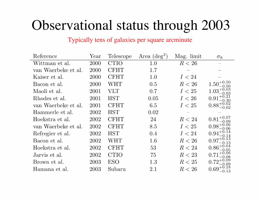
Observational status through 2003Typically tens of galaxies per square arcminute

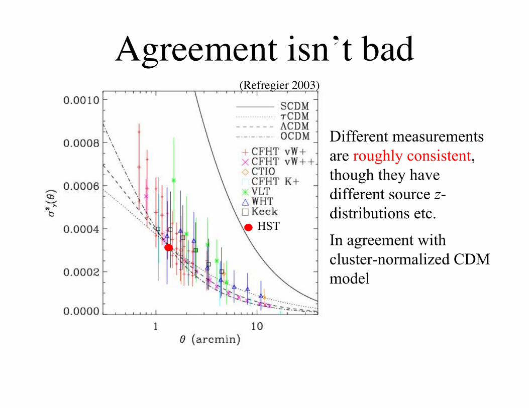
Agreement isn’t bad

Different measurementsare roughly consistent,though they havedifferent source z-distributions etc.

In agreement withcluster-normalized CDMmodel

HST

(Refregier 2003)

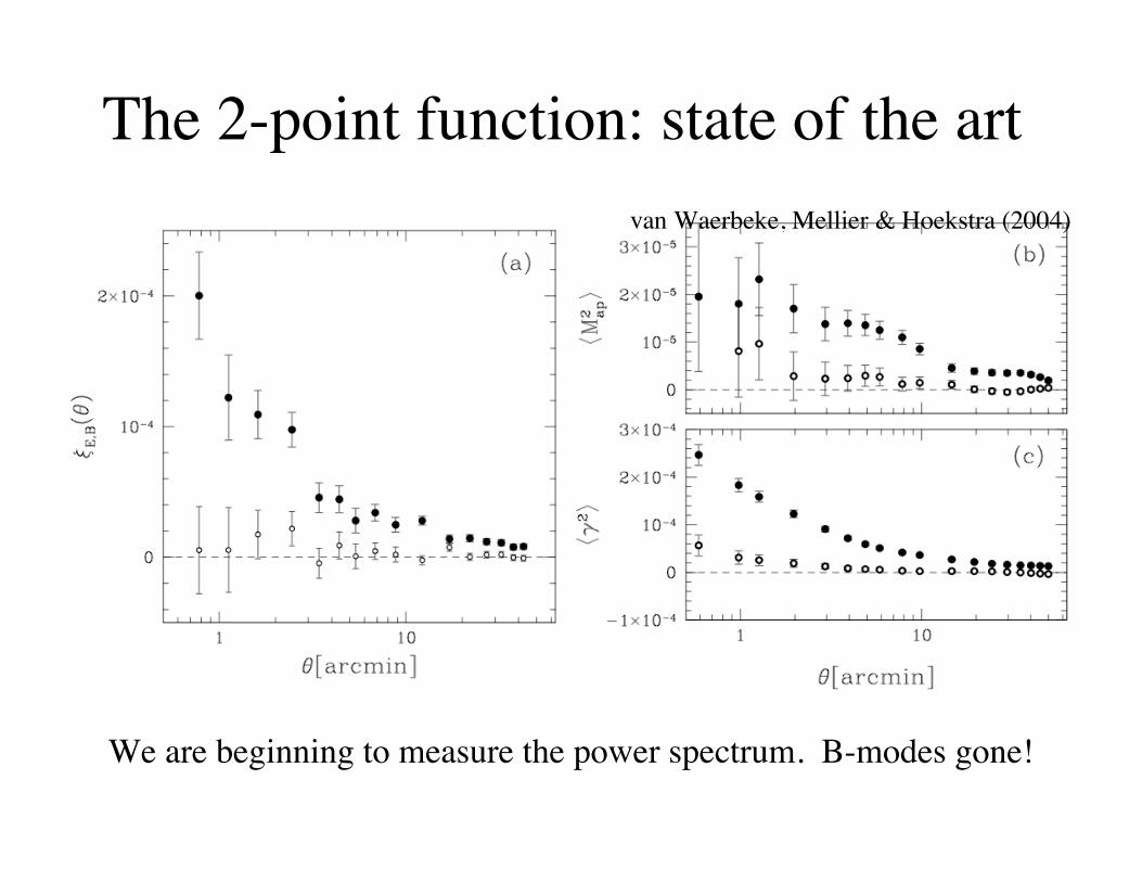
The 2-point function: state of the art

We are beginning to measure the power spectrum. B-modes gone!

van Waerbeke, Mellier & Hoekstra (2004)

CTIO surveyJarvis et al. (2005)

A 75 square degree lensingsurvey of ~ 2 milliongalaxies with 19<R<23.

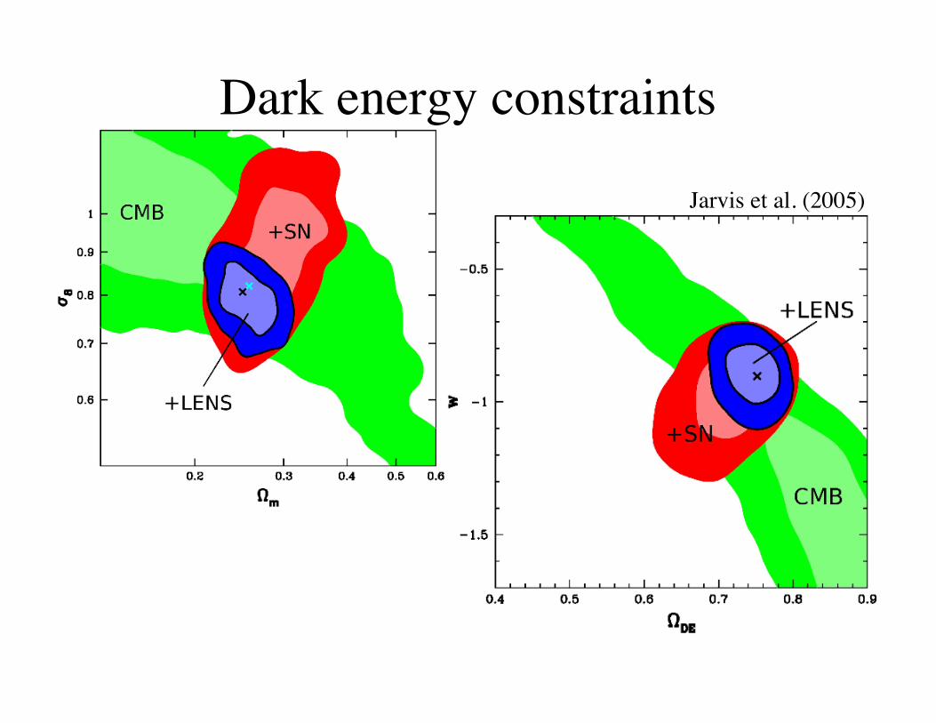
Dark energy constraints

Jarvis et al. (2005)

The CFHT legacy surveyHoekstra et al. (2006).First results from theCFHT-LS, covering 22square degrees.

See Schmid et al. (2006)for DE constraints.

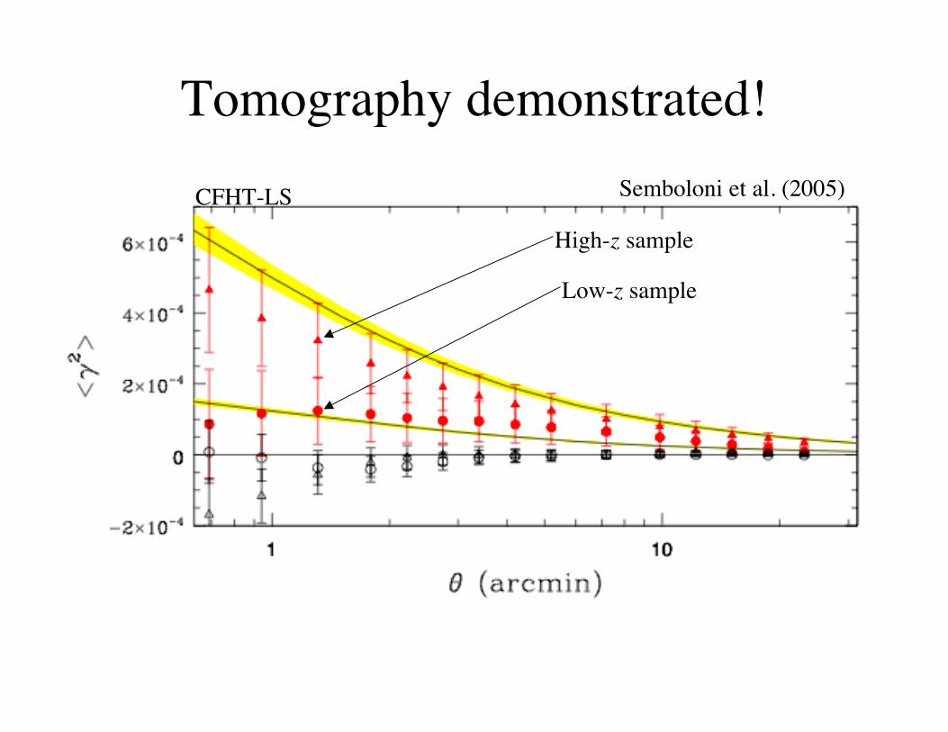
Tomography demonstrated!Semboloni et al. (2005)

High-z sample

Low-z sample

CFHT-LS

DETF report(Kolb et al.)

Finding 4d (of 15):WL also emerging technique. Eventual accuracy

will be limited by systematic errors that aredifficult to predict. If the systematic errors are ator below the level proposed by the proponents, itis likely to be the most powerful individualtechnique and also the most powerful componentin a multi-technique program.

Parameter Forecasts

Projected errors on thedark energy densityΩDE and the equationof state at the “pivot”redshift (where wp isuncorrelated with wa)for a “near future”survey.

From the DETF: Kolb et al.

The promise of space

A future space mission could, in principle, providestrong constraints on the equation of state of thedark energy, in addition to other science goals.

Galaxy number density & redshiftva

n W

aerb

eke,

Whi

te, H

oeks

tra &

Hey

man

s (20

06)

SpaceGrndSpaceGrnd(AB mag)

51443832262116118

1.4401.3581.2851.2161.1281.0440.9480.8690.787

2221.30728.51661.24828.01241.19627.5911.14327.0651.07626.5451.01926.0300.95125.5200.87925.0130.82524.5

ngal<zsrc>Depth

Future projects

200731,00041.8Pan-STARRS1

200?10,00024VISTA

201X20,0000.51.2Dune

201X1,000-5,0000.72SNAP

201X30,00078.4LSST

20095,0002.24DES

201131,0004x44x1.8Pan-STARRS4

20071,50012.6VST

200312013.6CFHT-LS

StartArea(deg2)

FOV(deg2)

Diameter(m)

Survey

Contributions to the error

van Waerbeke, White, Hoekstra & Heymans (2006)

Error, in units of thesignal, from:

• Sample variance• Redshift calibration• Shot noise

Simulations

Types and uses of simulations

• Halo abundances and shapes• Mass power spectra (and covariance matrices)• Projected mass maps• Ray tracing maps• Mock galaxy catalogues

We need numerical simulations to refine and calibrate algorithmsand analytic approximations, and potentially serve as templates

when the data become available.

Simulations can be used to extract:

Lensing lends itself to numerical simulation …

The MLP algorithm• The gold standard of simulation algorithms is the

“multiple lens plane” algorithm, where we traceray bundles through the evolving mass distributionin an N-body simulation.

• The lensing equations are discretized and theintegrals turned into sums:

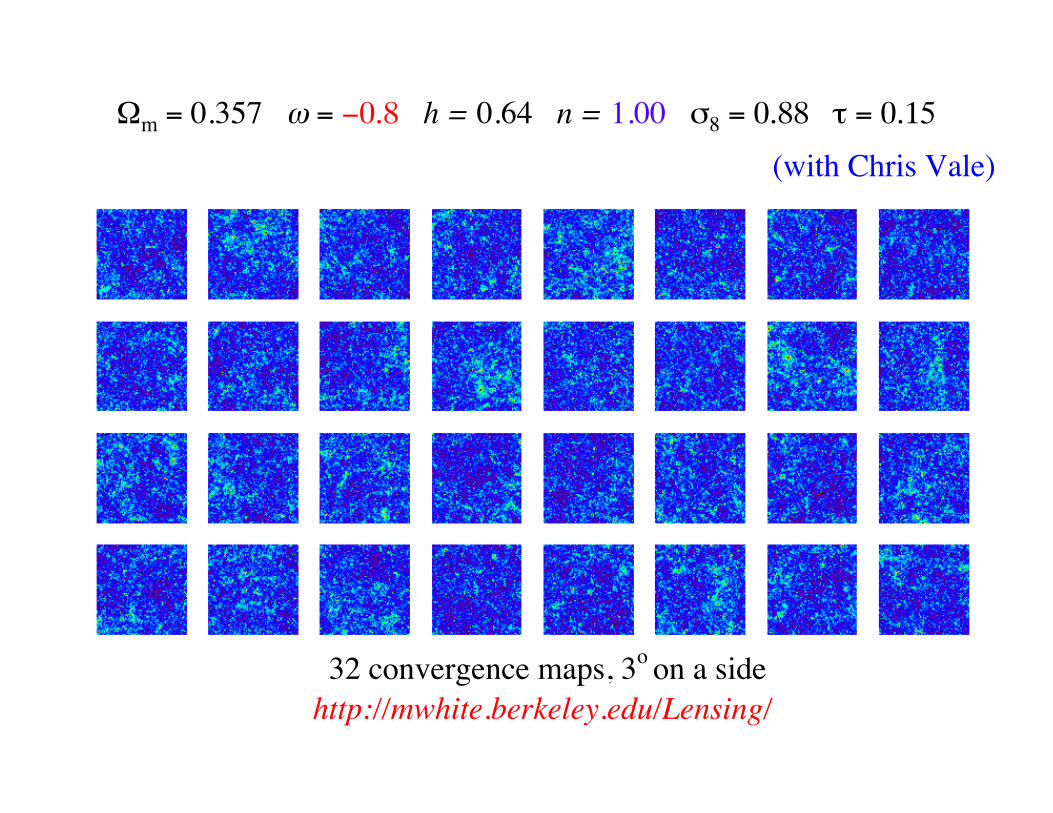
Ωm = 0.357 ω = −0.8 h = 0.64 n = 1.00 σ8 = 0.88 τ = 0.15

32 convergence maps, 3o on a sidehttp://mwhite.berkeley.edu/Lensing/

(with Chris Vale)

Numerical Effects: Resolution

• The effects of finiteresolution areunderstood

• We can predict thecost to achieve agiven accuracy

Force resolutionMass resolutionGrid resolutionTotal

Cl convergence study

(from Vale & White 2003)

All “theory” is simulation based(but different routes to final answer)

• Semi-analytic fits to powerspectra or halo profiles andmass functions vs. directsimulation.

• For 2-pt and 3-pt functions theagreement is good! (Goodenough?)

• Each method has differentstrengths and weaknesses.

Reduced shear• Unless we have a measurement of the intrinsic size or

magnification of a galaxy we cannot measure γ but onlyg=γ/(1-κ)

• Since γ and κ are usually small this difference is oftenneglected (except around clusters).

• Can be a few percent effect on arcminute scales!

Reducing shear enhances shear• On small scales κ can be quite large, and spatial

smoothing does not commute with the “reducing”operation.

• Generally g has larger fluctuations than γ becauseκ is skew positive.– Excess small-scale power compared to naïve

predictions.• The effect is different for different estimators

– A signal of “reduced shear” vs. e.g. intrinsic alignmentsor systematics.

• The effect is non-linear– Provides cross-check on shear calibration

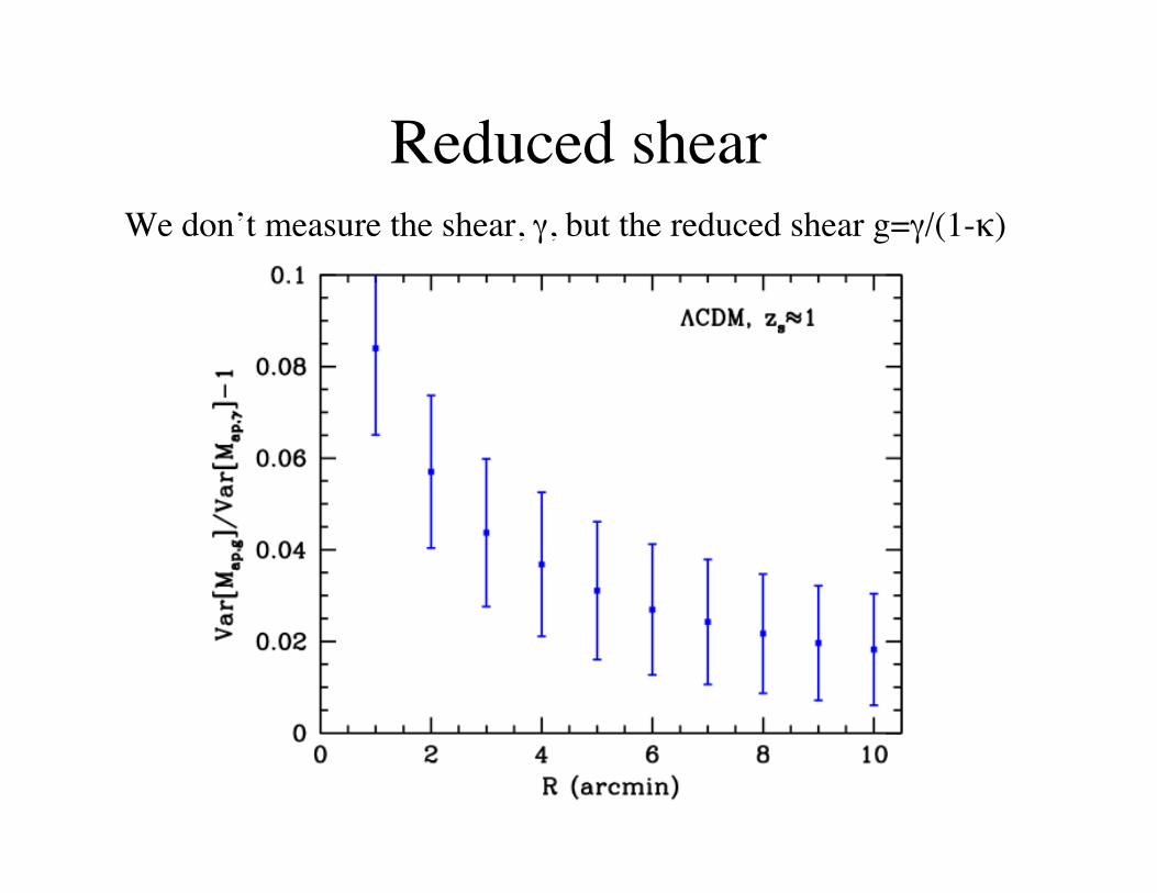
Reduced shearWe don’t measure the shear, γ, but the reduced shear g=γ/(1-κ)

A semi-analytic model

Dodelson, Shapiro & White (2005)

CFHT-LS

Bias in parameters

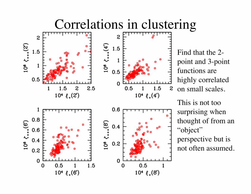
Correlations in clustering

Find that the 2-point and 3-pointfunctions arehighly correlatedon small scales.

This is not toosurprising whenthought of from an“object”perspective but isnot often assumed.

Correlations contd.• Correlation matrix for

2nd and 3rd order Mapstatistics (computedfrom κ maps).

• Uses Mexican hatfilter with scales 1, 2,4, 8 & 16 arcmin (40measures: 5x 2-pt and35x 3-pt).

Beyond N-bodyGravitational lensing is “simple” because it involves only gravity,albiet non-linear gravity. However non-gravitational physics doesbecome important on small scales:

• Hot baryons experience pressure forces which smooth outthe inner cusps in halo profiles.• Baryonic cooling produces steep inner cusps in galaxies,leading to strong (extreme) lensing events.• Contraction of baryons by cooling alters the potential inthe surroundings, changing the lensing signal.• Cooling alters the profiles of sub-halos, affecting lensing.

It is difficult to model these effects accurately at present, but wecan make toy models to guesstimate the size of the effects andrun simulations which allow for non-linear feedback.

Beyond gravity• Non-gravitational physics becomes important on

small scales, becoming dominant beyond l~3000.– White (2005), Zhan & Knox (2005), Jing et al. (2006).

Jing et al. (2006), usinghydro simulations -including feedback - findbaryons introduce ~1%uncertainty for l<103, inagreement with analyticpredictions.

Major sources of uncertainty• Source redshift distribution

– Problems with existing calibrations based on HDF• van Waerbeke, White, Hoekstra, Heymans (2006)

– Want multi-color photometry of all galaxies used.– New ideas for z-distribution calibration.

• Newman (2006)

• Theory– Modeling non-linearity– Non-gravitational effects– Intrinsic alignments

• Shear measurement procedure– Lots of progress with STEP, but a long way to go.– New “PCA” methods seem very promising.

The ultimate source screen …

Lensing of the CMBOf course galaxies aren’t the only source of (lensed) light in theuniverse. Any screen will do. Large-scale structure will lens theCMB anisotropy.Since we don’t know the “shape” of the CMB a priori we needto use more statistical information.

Quadratic estimator:if I have a field x with <x.x>=C=C0 + p C1 then a quadraticestimator of p is generically Qij xi xjRequiring this to be unbiased and minimum variance forGaussian x gives

Lensing of the CMB (contd)Now consider the CMB, lensed

The correlation function will depend on Φ, allowing us to make aquadratic estimator assuming everything is Gaussian and thedeflection angle is small.

(Hu; Hirata & Seljak)

We should be able to detect this effect with upcomingexperiments!Unfortunately the sky is not Gaussian enough and the deflectionsnot small enough to make this a 1% measurement.

The End

Recent reviews

• Mellier, 1999, ARA&A, 37, 127• Bartelmann & Schneider, 2001, Phys. Rep., 340, 291• Hoekstra, Yee & Gladders, 2002, New Astronomy

Reviews, 46, 767• Refregier, et al., 2003, ARA&A, 41, 645• van Waerbeke & Mellier, astro-ph/0305089