Weakly Ionized Plasmas in Hypersonics Sergey Macheret Department of Mechanical and Aerospace Engineering Princeton University 41 st Course: Molecular Physics and Plasmas in Hypersonics Erice, Sicily, Italy August 3, 2005
Transcript
Weakly Ionized Plasmas in Hypersonics
Sergey Macheret
Department of Mechanical and Aerospace EngineeringPrinceton University
41st Course: Molecular Physics and Plasmas in HypersonicsErice, Sicily, ItalyAugust 3, 2005
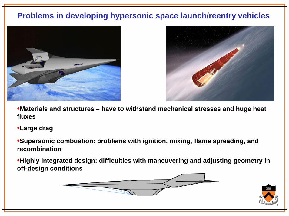
Problems in developing hypersonic space launch/reentry vehicles
•Materials and structures – have to withstand mechanical stresses and huge heat fluxes
•Large drag
•Supersonic combustion: problems with ignition, mixing, flame spreading, and recombination
•Highly integrated design: difficulties with maneuvering and adjusting geometry in off-design conditions
Aerospace Applications of Weakly Ionized Plasmas•Plasmas as a way of delivering energy to the flow (only heating, ionization per se is not critical):
•DC, AC, RF surface discharges (virtual shapes) for separation and turbulent transition control
•Virtual shapes created by off-body energy addition for drag reduction, steering, shock control, flow turning, using microwave and electron beams, laser sparks, and plasma jets
•Plasma-assisted combustion (thermal ignition)
•Ionization is critical in applications utilizing electromagnetic interactions:
•Forces exerted by B and E fields on charged particles (transferred to neutral gas by collisions): MHD power extraction and hypersonic flow control
•Reflection/absorption of electromagnetic waves (plasma Stealth; protection from EM weapons; communications)
•Plasma-assisted combustion (cold, non-thermal)
•At low T, artificial ionization is needed, and the power cost of ionization determines design and performance
•Power extraction from one region and its use in another region (MHD bypass):
•Can be very effective in managing energy, heat loads, and aerodynamics
•Performance limited by flow heating and losses of total pressure and (if in propulsion flowpath) thrust
Reverse Energy Bypass Concept
Directed energy steering
and possibledrag reduction
E-beam sustainedMHD shock angle
control
Magnetically drivenhigh repetition ratesnowplow arcs for
suppression of separation
MHD power extraction
Hr
Plasma generated virtual cowl lip for air
capture increase
Plasma energy additionfor elimination of isolator in
transient ramjet operation
Plasma/MHDenhanced mixing, flame spreading, and ignition control
3 LEVELS OF PLASMA/MHD MODELING•Kinetics:
•Non-local time-dependent electron energy distribution function in “forward-back” approximation, including high-energy runaway electrons, E and B fields, elastic & inelastic collisions.
•Drift-diffusion approximation for electrons and ions, including E and B fields, elastic & inelastic collisions, and plasma kinetics (ionization/recombination, attachment/detachment)
•Poisson equation for E field
•Vibrational excitation/relaxation
•Compressible fluid dynamics
•Single-fluid MHD model:
•Compressible fluid dynamics with E and B fields (jxB forces, power extraction, Joule dissipation)
• Energy deposition per pulse: 300 µJ, 350 µJ, and 360 µJ at 1, 5, and 10 Torr respectively
• The change in electron number density during the pulse measured previously using microwave diagnostics: 6×1011 cm-3 (±40%).
Combining all uncertainties, the ranges for the energy cost of electron generation:
Yi=55-125 eV/electron at 1 Torr, Yi=65-145 eV/electron at 5 Torr, and Yi=70-150 eV/electron at 10 Torr.
-10 -5 0 5 10 15 20 25 30 35 40-30
-20
-10
0
10
Ano
de C
urre
nt /
amps
Effect of High Voltage Pulse Across Static Cell
-10 -5 0 5 10 15 20 25 30 35 40-15000
-10000
-5000
0
5000
Cat
hode
Vol
tage
-10 -5 0 5 10 15 20 25 30 35 40-50
0
50
100
150
Pow
er /
kW
-10 -5 0 5 10 15 20 25 30 35 40
0
100
200
300
400
500
Ene
rgy
/ µjo
ules
Time / ns
High Pressure 1 Torr 5 Torr10 Torr
Test of ionization mechanisms at high E/N: left branch of the Paschen curvePaschen's Law (F. Paschen, Wied. Ann., 37, 69, 1889) for breakdown voltage: V= f(pd), where p is the pressure and d is the interelectrode distance.
B.N. Klyarfel’d, L.G. Guseva, 1964
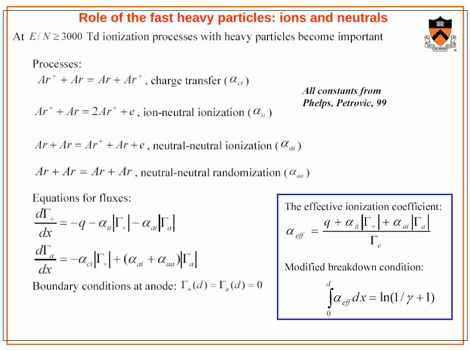
Role of the fast heavy particles: ions and neutrals
The Boltzmann kinetic equation in ‘forward-backward’ approximation
1 11 , 1 , 2 1 1
2( ) ( ) ( )s s m s s c ss ss
n meE N N Qt x M
σ ε σ ξε
∂ ∂Γ ∂+ + − Γ − Γ = Γ −Γ + Γ
∂ ∂ ∂ ∑ ∑2 2
2 , 2 , 1 2 22( ) ( ) ( )s s m s s c s
s ss
n meE N N Qt x M
σ ε σ ξε
∂ ∂Γ ∂− + Γ − Γ = Γ −Γ + Γ
∂ ∂ ∂ ∑ ∑
1,2 1,2( , , ) ( , , ) 2x t n x t mε ε εΓ =
1 2 e 1 2( , ) ( ) , ( , ) ( )en x t n n d x t dε ε= + Γ = Γ −Γ∫ ∫
Role of ionization by fast heavy particles at high E/p near cathode
0.0 0.2 0.4 0.6 0.8 1.010-26
10-23
10-20
10-17
10-14
10-11
10-8
10-5
10-2
101
Ar; V=Vmin=151.5 V; γ=0.07
αaiΓa
αiiΓ+
qel
q el, α
iiΓ+, α
aiΓ a
, 1/c
m3 se
c (p
er Γ
e(0)=
1)
px, Torr*cm0.0 0.1 0.2 0.3
10-5
10-4
10-3
10-2
10-1
100
101
102
103
Ar; V=Vmin=1175 V; γ=0.07
αaiΓaαiiΓ+
qel
q el, α
iiΓ+, α
aiΓ a
, 1/c
m3 se
c (p
er Γ
e(0)=
1)
px, Torr*cm
V
pd
E/p=151.5 V/cm/Torr
V
pdE/p=3916 V/cm/Torr
Electron energy distribution function:
runaway at high E/p
0 50 100 150 200
xp=0.75
0 50 100 150 200
xp=0.5
n(ε,x), cm3/eV
0 50 100 150 2001x10-13
1x10-12
1x10-11
1x10⁻¹⁰
1x10⁻⁹
Ar; E/p=151.5 V/cm*Torrpd=1 Torr*cm
xp=0.25 cm*Torr
ε, eV
0 50 100 150 200
xp=0.95
0 200 400 600 800 1000 1200
0.75pd
0 200 400 600 800 1000 1200
0.5pd
n(ε,x), cm3/eV
0 200 400 600 800 1000 1200
1x10-12
1x10-11
1x10⁻¹⁰
1x10⁻⁹
Ar; E/p=3916.6 V/cm*Torrpd=0.3 Torr*cm
0.25pd
ε, eV
0 200 400 600 800 1000 1200
0.95pd
100
1000
0 1 2 3 4 5
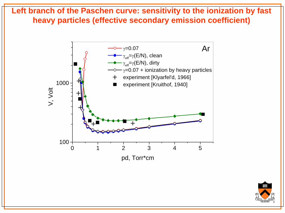
γ=0.07 γeff=γ(E/N), clean γeff=γ(E/N), dirty γ=0.07 + ionization by heavy particles experiment [Klyarfel'd, 1966] experiment [Kruithof, 1940]
Ar
pd, Torr*cm
V, V
olt
Left branch of the Paschen curve: sensitivity to the ionization by fast heavy particles (effective secondary emission coefficient)
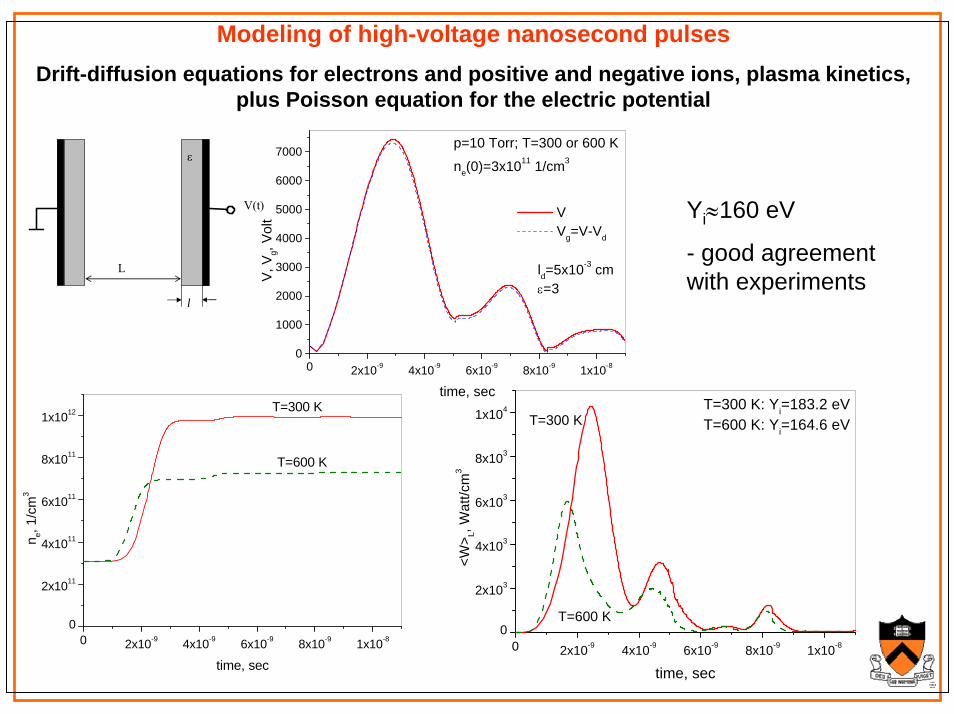
Modeling of high-voltage nanosecond pulsesDrift-diffusion equations for electrons and positive and negative ions, plasma kinetics,
plus Poisson equation for the electric potential
0 2x10⁻⁹ 4x10⁻⁹ 6x10⁻⁹ 8x10⁻⁹ 1x10-80
1000
2000
3000
4000
5000
6000
7000
ld=5x10⁻³ cmε=3
V Vg=V-Vd
p=10 Torr; T=300 or 600 K
ne(0)=3x10¹¹ 1/cm3
V, V
g, Vo
lt
time, sec
ε
L
l
V(t)
0 2x10⁻⁹ 4x10⁻⁹ 6x10⁻⁹ 8x10⁻⁹ 1x10⁻⁸
0
2x10¹¹
4x10¹¹
6x10¹¹
8x10¹¹
1x10¹² T=300 K
T=600 K
n e, 1/
cm3
time, sec0 2x10⁻⁹ 4x10⁻⁹ 6x10⁻⁹ 8x10⁻⁹ 1x10⁻⁸
0
2x10³
4x10³
6x10³
8x10³
1x10⁴
T=300 K
T=600 K
T=300 K: Yi=183.2 eVT=600 K: Yi=164.6 eV
<W> L,
Wat
t/cm
3
time, sec
Yi≈160 eV
- good agreement with experiments
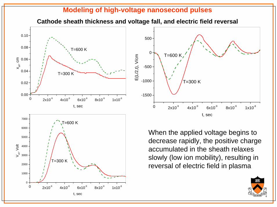
Modeling of high-voltage nanosecond pulsesCathode sheath thickness and voltage fall, and electric field reversal
0 2x10⁻⁹ 4x10⁻⁹ 6x10⁻⁹ 8x10⁻⁹ 1x10-80
1000
2000
3000
4000
5000
6000
7000
T=300 K
T=600 K
V sh, V
olt
t, sec
0 2x10⁻⁹ 4x10⁻⁹ 6x10⁻⁹ 8x10⁻⁹ 1x10-80.00
0.02
0.04
0.06
0.08
0.10
T=600 K
T=300 K
x sh, c
m
t, sec 0 2x10⁻⁹ 4x10⁻⁹ 6x10⁻⁹ 8x10⁻⁹ 1x10⁻⁸
-1500
-1000
-500
0
500
T=300 K
T=600 K
E(L
/2,t)
, V/c
m
t, sec
When the applied voltage begins to decrease rapidly, the positive charge accumulated in the sheath relaxes slowly (low ion mobility), resulting in reversal of electric field in plasma
Modeling of high-voltage nanosecond pulsesParametric studies with trapezoidal pulses: Role of pulse rise/fall time
Air; L=3 cm; p=10 Torr, γ=0.05, no ionization due to fast ions and molecules
0.0 5.0x10⁻¹⁰ 1.0x10⁻⁹ 1.5x10⁻⁹ 2.0x10-90
5000
10000
15000
20000
25000
V, V
olt
t, sec
ne(0)= 5×1011 cm-3, ne,max=1.1×1013 cm-3. Depending on τf, peak voltage was set so as to give the prescribed value of ne,max
0.0 0.1 0.2 0.3 0.4 0.5 0.6 0.7 0.8
60
80
100
120 f=100 kHz
ne(0)=5x10¹¹ 1/cm3
ne,max=1.1x10¹³ 1/cm3
<ne>1/f=2.12x1012 1/cm3Yi(ne,max)
Yi,
eV
τf, ns
13
14
15
16
17
<P>1/f
<P> 1/
f, W
att/c
m3
High-voltage nanosecond pulses: electron cost in the sheath and plasma•Glow discharge: E/N in sheath close to Stoletov’s point – efficient ionization; E/N in plasma positive column – low, high ionization cost
•High-V pulse: E/N in sheath far above Stoletov’s optimum – runaway electrons, inefficient ionization; E/N in plasma column – close to Stoletov’s optimum, efficient ionization
•High ionization efficiency in high-V pulses: optimum ionization occurs in the volume rather than in the thin sheath
0.000 0.025 0.050 0.075 0.100 0.125
100
1000
Yi(x,t)=abs(E(x,t)/α(x,t))
0.25 ns 0.5 ns 0.75 ns 1.0 ns 1.25 ns
Y i(x,t)
, eV
x, cmProfiles of the “local” cost of ionization at different moments of time for a model trapezoidal pulse
10-15 10-14 10-13101
102
103
104
DC or RFplasma
e-beam
(E/N)c
Y i, eV
E/N, V.cm2
MHD power extraction from an externally ionized, cold, supersonic air flow
BU
AluminumLexanKapton
1.2"x2"Test Section
Pulser
Load
U
Plasma Camera
The supersonic flow (Mach 3, 110 K,30 Torr) is ionized via a high repetition rate, high voltage, short pulse duration power supply (100 kHz, 30 kV, and 2.5 ns respectively) which generates an electron number density that peaks at ~ 1012 cm-3.
The electric discharge is uniform in the core flow between the electrodes with no arcing through the boundary layer. The MHD power extraction electrodes extend into the flow fromthe top and bottom walls of the channel
First Experimental Demonstration of MHD Effect in Cold Supersonic Air Flow With External Ionization
-5 0 5 10 15-0.50
0.51
1.5
Time / microsec
Cur
rent
/ma
15
Cur
rent
/ma
(Sm
ooth
ed)
Faraday Current in Measured Direction
-5 0 5 1000.10.20.30.40.5
Time / microsec
-5 0 5 10 15-0.50
0.51
1.5
-0.50
0.51
1.5
Time / microsec
Cur
rent
/ma
15
Cur
rent
/ma
(Sm
ooth
ed)
Faraday Current in Measured Direction
-5 0 5 1000.10.20.30.40.5
00.10.20.30.40.5
Time / microsec
To photomultiplier(Faraday Current)
UB
U x B
30 kV Pulser
2kΩ
Pulser CurrentMeasurement
1.2Ω
2kΩTo photomultiplier(Faraday Current)
UB
U x B
30 kV Pulser
2kΩ
Pulser CurrentMeasurement
1.2Ω
2kΩ
The current flowing through the plasma is monitored by a photo diode so that only current flowing in one direction is observed by the optically coupled photodetector
Current in reverse direction
The peak extracted current is 0.4 milliamps, and reverses with magnetic field reversal.
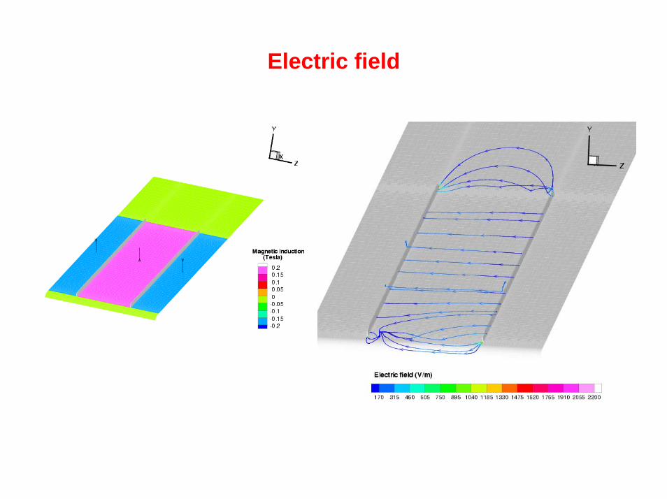
Modeling plasma kinetics and dynamics in the MHD section
•Quasi-1D in the y-direction (direction of Faraday e.m.f. and current)•Calculations for experimental conditions: p=10 Torr; T=106 K; u=620 m/s; B=5 T•3 cm spacing between MHD electrodes•Hall and ion slip effects included•Solve continuity equations for plasma electrons and positive and negative ions, plus the Poisson equation for the electric potential
Electron mobility, Hall parameter, and rates of recombination and attachment depend on electron temperature and, therefore, on E/N
0d
From experimental data in literature:( ) v ( / ) /( / ), ( / )e e eff eff e e effT N E N E N T T E Nµ = =
2
Hall effect, no ion slip:
for ideally segmented electrodes
for continuous electrodes1
eff
e
ENE
ENN
⎧⎪⎪= ⎨⎪⎪ +Ω⎩
2 2 2
With ion slip:
, where
is the electron current
outside the cathode sheath
eeff e
e x y z
E u BE jN Nj j j j j
σ
+ ×=
= + +
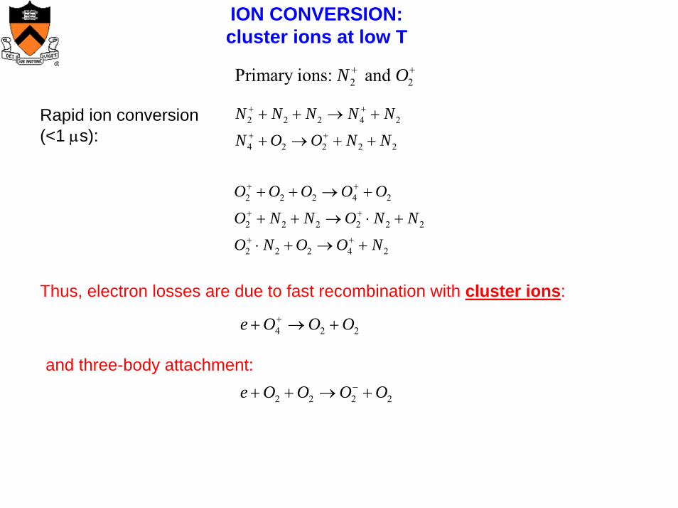
ION CONVERSION: cluster ions at low T
2 2Primary ions: and N O+ +
Rapid ion conversion (<1 µs):
2 2 2 4 2
4 2 2 2 2
2 2 2 4 2
2 2 2 2 2 2
2 2 2 4 2
N N N N N
N O O N N
O O O O O
O N N O N N
O N O O N
+ +
+ +
+ +
+ +
+ +
+ + → +
+ → + +
+ + → +
+ + → ⋅ +
⋅ + → +
Thus, electron losses are due to fast recombination with cluster ions:
4 2 2e O O O++ → +
and three-body attachment:
2 2 2 2e O O O O−+ + → +
MODELING OF PLASMA DYNAMICS AFTER THE PULSE IN CONTINUOUS-ELECTRODE FARADAY GENERATOR
•Current decay after the pulse is due to dissociative recombination with cluster ions and to three-body attachment (comparable contributions)
•Very good agreement with experiment
•Inferred peak electron density: 5×10¹¹ - 1012 cm-3 (excellent agreement with microwave transmission measurements in static cell)
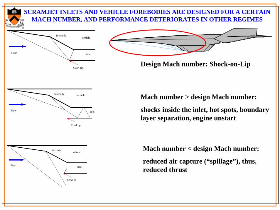
SCRAMJET INLETS AND VEHICLE FOREBODIES ARE DESIGNED FOR A CERTAIN MACH NUMBER, AND PERFORMANCE DETERIORATES IN OTHER REGIMES
vehicle forebody
Flow inlet
Cowl lip
vehicle forebody
Flow inlet
Cowl lip
Design Mach number: Shock-on-Lip
Mach number > design Mach number:
shocks inside the inlet, hot spots, boundary layer separation, engine unstart
Mach number < design Mach number:
reduced air capture (“spillage”), thus, reduced thrust
vehicle forebody
Flow inlet
Cowl lip
y
z
flow
electrodes
jy
Inlet shock control with on-ramp MHD generator
z y
xinlet
B e-beamjy
jxB
e-beam guns andmagnets
Flow
Bottom View
Single LargeMagnet
e-BeamsFlowpath
Magnete-Beams
Side Wall Electrodes
jy
Electron beam-generated heating
and ionization profiles:•“Forward-back” kinetic modeling
•Monte Carlo simulations
•Gaussian approximation of profiles
2 2
Quasi-Gaussian e-beam power deposition profile:
( ) exp( 2( ) / )b mbQ a z ww
ξ ξ= + − −
where ( ) ; / 3.21; 1.64 ; ( , ) is the beam relaxation length
b m R m
R b
z x z z L w zL N
ξε
= − ≈ ≈
1.7211.1 10 / , mR bL Nε= ⋅
0
Conditions for , : ( ) 0 and ( ) /RL
b R b b ba b Q L Q d j eξ ξ ε= =∫21 1/1.7
0
1( ) ( , ) ; ( ) ( /1.1 10 )RL
b RR
N x N x d x L NL
ξ ξ ε= = ⋅∫Ionization rate: ( , ) ( , ) /( ), where 34 eVi b i iq x Q x eW Wξ ξ≈ =
0 2 4 6 8 10 12 140.00
0.05
0.10
0.15
0.20
MCC (Cyltran); B=7 T Gauss appr. with LR(εb,N) Gauss appr. with LR from MCC
p=76 Torr; εb=25 keV
Qb,
rel.u
nits
z, cm
Model includes:
•2D marching inviscid CFD code plus uncoupled boundary layer calculation
•MHD equations
•E-beam ionization and power profiles
•Plasma kinetics
•Vibrational excitation and relaxation
THE MODEL
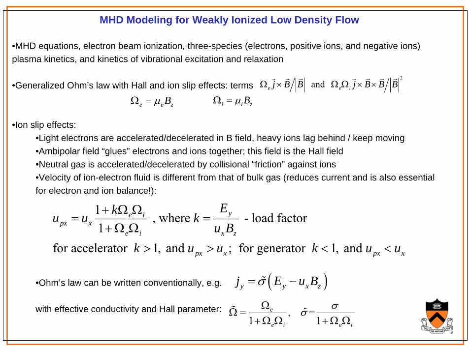
MHD Modeling for Weakly Ionized Low Density Flow
•MHD equations, electron beam ionization, three-species (electrons, positive ions, and negative ions) plasma kinetics, and kinetics of vibrational excitation and relaxation
•Generalized Ohm’s law with Hall and ion slip effects: terms
•Ion slip effects:•Light electrons are accelerated/decelerated in B field, heavy ions lag behind / keep moving•Ambipolar field “glues” electrons and ions together; this field is the Hall field•Neutral gas is accelerated/decelerated by collisional “friction” against ions•Velocity of ion-electron fluid is different from that of bulk gas (reduces current and is also essential for electron and ion balance!):
•Ohm’s law can be written conventionally, e.g.
with effective conductivity and Hall parameter: , =1 1
e
e i e i
σσΩΩ =
+Ω Ω +Ω Ω
( )y y x zj E u Bσ= −
2 and e e ij B B j B B BΩ × Ω Ω × ×
e e zBµΩ = i i zBµΩ =
1 , where - load factor1
for accelerator 1, and ; for generator 1, and
ye ipx x
e i x z
px x px x
Eku u ku B
k u u k u u
+ Ω Ω= =
+Ω Ω
> > < <
MHD Modeling for Weakly Ionized Low Density Flow
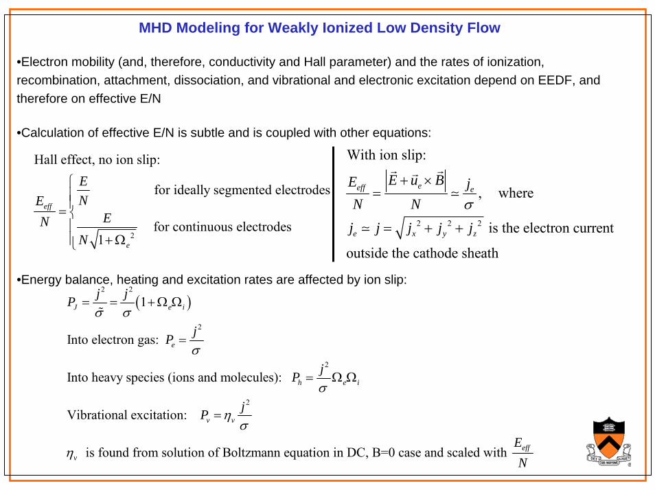
•Electron mobility (and, therefore, conductivity and Hall parameter) and the rates of ionization, recombination, attachment, dissociation, and vibrational and electronic excitation depend on EEDF, and therefore on effective E/N
•Calculation of effective E/N is subtle and is coupled with other equations:
•Energy balance, heating and excitation rates are affected by ion slip:
2
Hall effect, no ion slip:
for ideally segmented electrodes
for continuous electrodes1
eff
e
ENE
ENN
⎧⎪⎪= ⎨⎪⎪ +Ω⎩
( )2 2
2
2
2
1
Into electron gas:
Into heavy species (ions and molecules):
Vibrational excitation:
is found from solution of Boltzmann equation in DC, B=0 case and
J e i
e
h e i
v v
v
j jP
jP
jP
jP
σ σ
σ
σ
ησ
η
= = +Ω Ω
=
= Ω Ω
=
scaled with effEN
2 2 2
With ion slip:
, where
is the electron current
outside the cathode sheath
eeff e
e x y z
E u BE jN Nj j j j j
σ
+ ×=
= + +
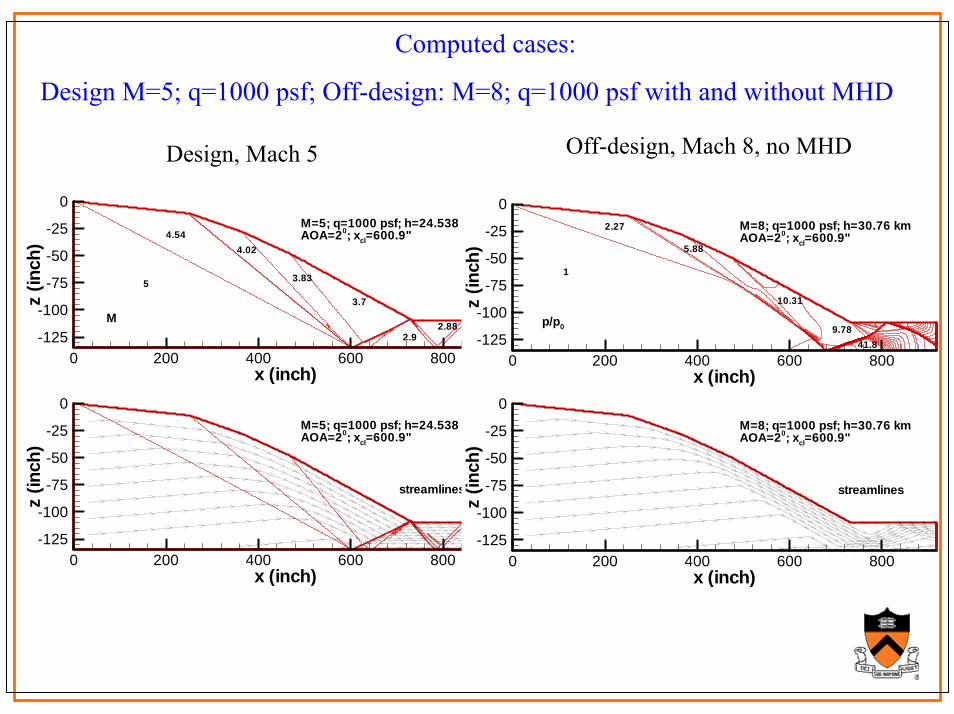
Computed cases:
Design M=5; q=1000 psf; Off-design: M=8; q=1000 psf with and without MHD
x (inch)
z(in
ch)
0 200 400 600 800-125
-100
-75
-50
-25
0M=5; q=1000 psf; h=24.538 kmAOA=20; xcl=600.9"
M
5
4.544.02
3.83
3.7
2.92.88
x (inch)
z(in
ch)
0 200 400 600 800-125
-100
-75
-50
-25
0M=5; q=1000 psf; h=24.538 kmAOA=20; xcl=600.9"
streamlines
x (inch)
z(in
ch)
0 200 400 600 800-125
-100
-75
-50
-25
0M=8; q=1000 psf; h=30.76 kmAOA=20; xcl=600.9"
p/p0
1
2.27
5.88
10.31
9.7841.8
x (inch)
z(in
ch)
0 200 400 600 800-125
-100
-75
-50
-25
0M=8; q=1000 psf; h=30.76 kmAOA=20; xcl=600.9"
streamlines
Design, Mach 5 Off-design, Mach 8, no MHD
Inlet shock control with on-ramp MHD generator: restoration of shock-on-lip condition at Mach 8, 1000 psf (design – Mach 5)
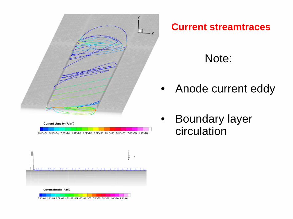
Current reversal and flow acceleration should exist in boundary layers of MHD generators: effects on vorticitygeneration, flow separation, and turbulent transition
MHD Aerodynamic Control and Thrust Vectoring ConceptElectromagnets
and e-beam guns
B
e-beam
jxB
z y
x
Flow
inlet
y
z E-beams On E-beams Off
electrodes
Rear view
y
z
x jxB
j
E-beam gun
Bottom view
jxB
exhaust
Turning moment
x
y
jxB
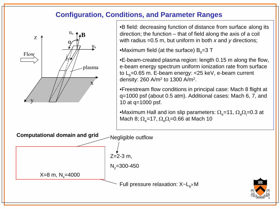
Configuration, Conditions, and Parameter Ranges
z
y
x
uz
plasma
ux
Flow
B
jy
α
•B field: decreasing function of distance from surface along its direction; the function – that of field along the axis of a coil with radius =0.5 m, but uniform in both x and y directions;
•Maximum field (at the surface) B0=3 T
•E-beam-created plasma region: length 0.15 m along the flow, e-beam energy spectrum uniform ionization rate from surface to Lb=0.65 m. E-beam energy: <25 keV, e-beam current density: 260 A/m2 to 1300 A/m2.
•Freestream flow conditions in principal case: Mach 8 flight at q=1000 psf (about 0.5 atm). Additional cases: Mach 6, 7, and 10 at q=1000 psf.
•Maximum Hall and ion slip parameters: Ωe=11, ΩeΩi=0.3 at Mach 8; Ωe=17, ΩeΩi=0.66 at Mach 10
Computational domain and grid
X=8 m, Nx=4000
Z=2-3 m,
Nz=300-450
Negligible outflow
Full pressure relaxation: X~Lb×M
Electron number density and electrical conductivity
Profiles of j×B forces at χ=0.25, 0.5, and 1: accelerator, Mach 8, α=π/2, Qb=10 MW/m3
x , m
z,m
-0.5 -0.25 0 0.25 0.50
0.2
0.4
0.6
0.8
1f=jxB; Ey=0.25u0B0
x , mz
,m
-0.5 -0.25 0 0.25 0.50
0.2
0.4
0.6
0.8
1f=jxB; Ey=0.5u0B0
x , m
z,m
-0.5 -0.25 0 0.25 0.50
0.2
0.4
0.6
0.8
1f=jxB; Ey=u0B0
Drag/thrust force Fx and MHD-deposited power PMHDversus parameter χ
0.2 0.4 0.6 0.8 1.0 1.2
-2000
-1000
0
1000
2000
3000
4000 Accelerator: Qb=10 MW/m3; Pb=0.966 MW/m
Lb=0.65 m; α=π/2
F x, N
/m
χ=Ey,el/u0B0
0
5
10
15
20
25
30
PMHD
Fx
PM
HD, M
W/m
j=σ(E-uB). E is global (uniform), but uB varies. Thus, depending on parameter χ=Ey/(u0B0), current and j×B forces can reverse direction within MHD region
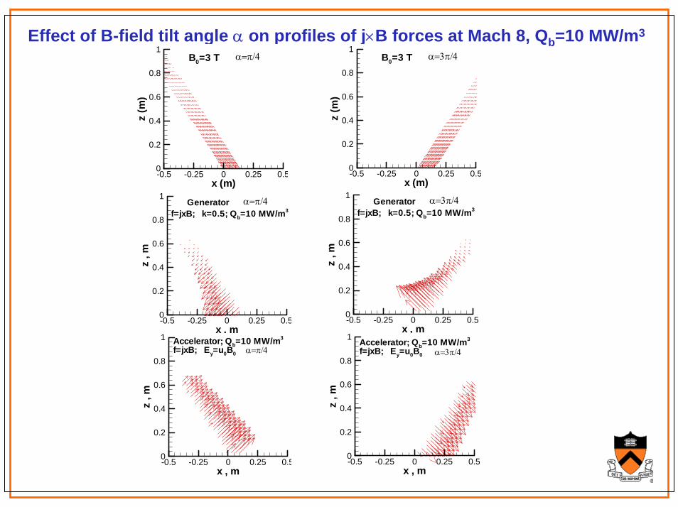
Effect of B-field tilt angle α on profiles of j×B forces at Mach 8, Qb=10 MW/m3
x (m)
z(m
)
-0.5 -0.25 0 0.25 0.50
0.2
0.4
0.6
0.8
1B0=3 T α=π/4
x (m)
z(m
)
-0.5 -0.25 0 0.25 0.50
0.2
0.4
0.6
0.8
1B0=3 T α=3π/4
x , m
z,m
-0.5 -0.25 0 0.25 0.50
0.2
0.4
0.6
0.8
1
f=jxB; k=0.5; Qb=10 MW/m3α=π/4Generator
x , mz
,m-0.5 -0.25 0 0.25 0.50
0.2
0.4
0.6
0.8
1
f=jxB; k=0.5; Qb=10 MW/m3α=3π/4Generator
x , m
z,m
-0.5 -0.25 0 0.25 0.50
0.2
0.4
0.6
0.8
1 Accelerator; Qb=10 MW/m3
f=jxB; Ey=u0B0 α=π/4
x , m
z,m
-0.5 -0.25 0 0.25 0.50
0.2
0.4
0.6
0.8
1 Accelerator; Qb=10 MW/m3
f=jxB; Ey=u0B0 α=3π/4
Normal force ∆L and lift-to-drag or lift-to-thrust ratio ∆L/∆D or ∆L/∆T
for generator (k=0.5) and accelerator (χ=1) at Mach 8, at tilt angle α=π/2 versus Qb, and at Qb=10 MW/m3 versus α
10 20 30 40 503x103
4x10³
5x10³
6x10³
7x10³
8x10³
9x10³
1x10⁴
1x10⁴
Lb=0.65 m; α=π/2
Generator: k=0.5
∆L, N
/m
Qb, MW/m3
1.9
2.0
2.1
2.2
2.3
2.4
2.5
2.6
∆L/∆
D
Lplate=8 m
0.25 0.50 0.751500
2000
2500
3000
3500
4000
πππ
∆L, N
/m
tilt angle α, radian
1.5
2.0
2.5
3.0
3.5
Lplate=8 m Lb=0.65 m; Qb=10 MW/m3
∆L/∆
D
Generator: k=0.5
10 20 30 40 50
6.0x10³
8.0x10³
1.0x10⁴
1.2x10⁴
Lb=0.65 m; α=π/2
Accelerator: Ey=u0B0
∆L, N
/m
Qb, MW/m3
1.950
1.955
1.960
1.965
1.970
1.975
∆L/∆
D
Lplate=8 m
0.25 0.50 0.752000
2200
2400
2600
2800
3000
πππ
∆L, N
/m
tilt angle α, radian
2.0
2.5
3.0
3.5
Lb=0.65 m; Qb=10 MW/m3
∆L/∆
D
Accelerator: Ey=u0B0
Magnetically driven snowplow surface arc for boundary layer control:
Lab setup
Superconducting magnet withdischarge
diffuser Inlet and nozzle
Sidewall electrodes in the test section
Flow Direction
2.0 inches
Part of tunnel holders (not relevant)
Experimental Results
Flow: Mach 3 (600 m/s)
1.0 µs exposure
10 µs exposure
50 µs (left) and 20 µs (right) exposure
B=0: Arc velocity = 425 m/s
B=2 Tesla: Arc velocity = 3,000-5,000 m/s
Flow: Mach 3, u=600 m/s
•Plasma velocity:
Physics of magnetically driven cold snowplow arc
--
++
j×Bnn
Polarization (Hall) field
Collisional(friction) forces
( ), ,
9 3
, ,
where - reduced mass (ion-neutral), 0.9 10 cm / s - rate constant of ion-neutral collisions, and - plasma and gas velocities ( )
in i e i in i e i
in
e i e i
jB M k n n u V M k n nu
M ku V u V
−
′ ′= −
′ ≈ ×
•After transformation:, 1
e ie i
e i
EuB
Ω Ω=
+Ω ΩAt B=2 T, E=1.5 kV/cm: ue,i=3000-5000 m/s – agrees with experimental data.This is true for thin plasma column, especially in its middle. Closer to electrodes, Hall effect plays a role. If the Hall current flows freely:
2 21 1
, 2
; ;
1
e
e e
jj
e ie i
e i e
j j
EuB
Ω⊥ +Ω +Ω= =
Ω Ω=
Ω Ω + +Ω
, ,1: e e i i dr iin
E eEu VB M ν
Ω ≈ Ω = =′
•Electrons are pulled by the Lorentz force, trying to break away from ions
•The ambipolar (polarization) E-field glues electrons and ions together
•The ion-electron fluid experiences collisional “friction” against neutral gas
•Ion “friction” imparts momentum to the bulk gas
•Arc velocity: V=(E/B)ΩeΩi/(1+ ΩeΩi), where Ωe and Ωi are electron and ion Hall parameters (ratios of cyclotron frequency to the collision frequency)
•V=2-5 km/s at B=1-2 T (good agreement with measurements)
•Arc canting due to Hall effect
•Gas velocity increment in a single run of the arc: ∆v~0.3 m/s
•Each gas element, as it traverses the ~1’’ interaction region, is overcome and hit by fast-moving consecutive arcs many times, thus velocity deep in the boundary layer increases by ~25-100 m/s(consistent with measurements)
•Closer to the wall, velocity is lower, and the gas experiences more arc strikes, thus accelerating stronger than the gas far from the surface. This “swells” boundary layer velocity profile (good)
•(Push work)/(Joule dissipation)<<1. However, ~25-50% of Joule dissipation is channeled into vibrational excitation of nitrogen and convected downstream. The estimated ∆T is ~30-80 K. Minimization of heating by additional ionization?
• The magnetically driven cold snowplow arc is promising for separation and turbulence control
Physics of magnetically driven cold snowplow arc
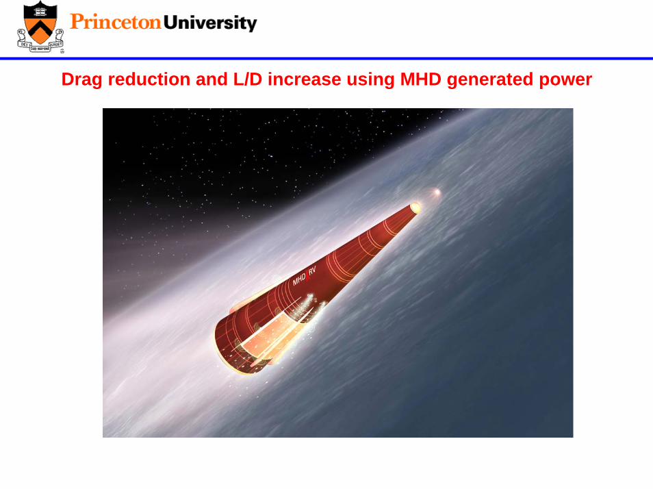
MHD POWER GENERATION AND AERODYNAMIC CONTROL FOR REENTRY VEHICLES
Flight configuration
Seed injection slot
MHD region
Flight configuration
Seed injection slot
MHD region
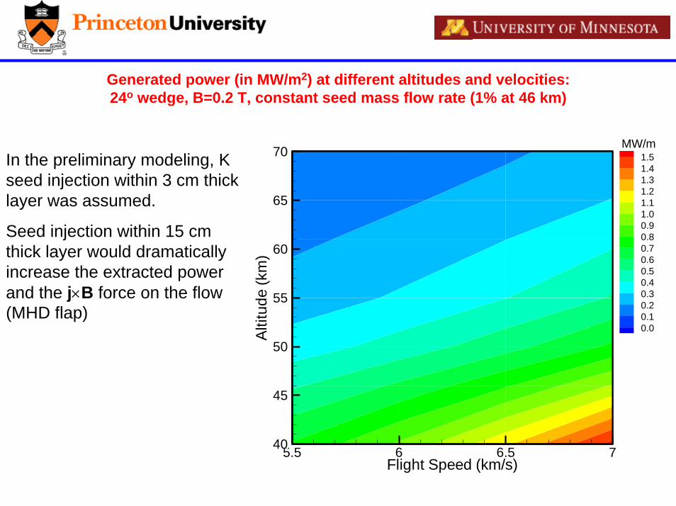
Can large amounts of electric power be extracted from the boundary layer with MHD generators on board reentry vehicles? Can the power be used
for aerodynamic control?
PRELIMINARY ANALYSIS: CONDUCTIVITY
The scalar electrical conductivity ( )2
e
en ei
e nm
σν ν
=+
3 2 510 10 : 2.7 10 mho/me en nn n
σ− −≤ − ≈ ×
It is in this regime that the conductivity of unseeded air in the boundary layer
at T=4,000 – 5,000 K reaches ~10 mho/m.3/ 2
210 : ln
e en Tconstn
σ−≥ = ×Λ
This regime will exist in the boundary layer with Te=T=4,000 – 5,000 K and with ~1% of alkali vapor. At this temperature alkali atoms will be almost fully ionized, and the scalar conductivity of about 600-1000 mho/m will be achieved.
POWER GENERATION WITH HALL AND ION SLIP EFFECTS
Maximum MHD power per unit volume 2 2max
14 effP u Bσ=
2
for ideal Faraday generators
= for continuous-electrode Faraday generators1+
effσ σ
σ
=
Ω
The effective conductivity:
Scalar conductivity and Hall parameter corrected for ion slip:
( ), , electron and ion Hall parameters: ,
1 1e
e ie i e i en ei in
eB eBm M
σσν ν ν
Ω= Ω = Ω = Ω =
+Ω Ω +Ω Ω +
( )
2 2
max
2 222
1 for ideal Faraday generators4 1
11 = for continuous-electrode Faraday generators4 1
e i
e i
e e i
u BP
u B
σ
σ
=+Ω Ω
+Ω Ω
Ω + +Ω Ω
Thus:
MAXIMUM MHD POWER PER UNIT VOLUME VS. B FIELD,
WITH HALL AND ION SLIP EFFECTS
0 2 4 6 8 10 12 14101
102
103
104
Pmax,cont
Pmax,segm
P max
,seg
m, P
max
,con
t, M
W/m
3
B, T
0.0 0.2 0.4 0.6 0.80
100
200
300
400
500
Pmax,cont
Pmax,segm
B, T
0 2 4 6 8 10 12 1410-5
10-4
10-3
10-2
10-1
100
101
102
Ωe>>1; ΩeΩi>1Ωe>>1; ΩeΩi<1Ωe<<1
Ωe/(1+ΩeΩi)
ΩeΩi
Ωe
Ωe, Ω
e/(1+
ΩeΩ
i), Ω
eΩi
B, T
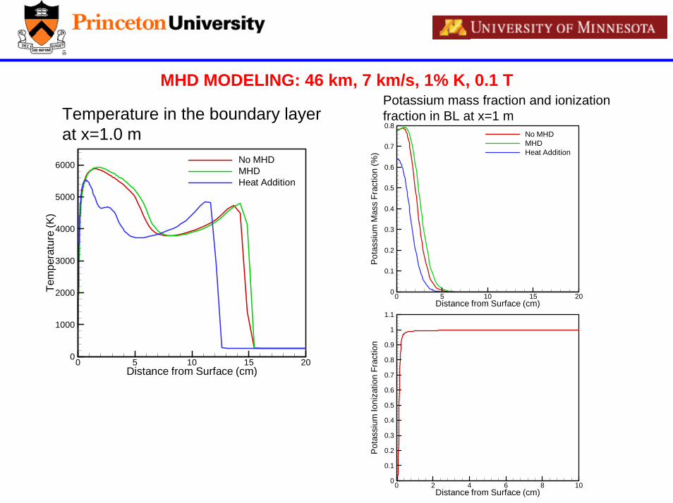
Flight: 46 km, 7 km/s. Bound. layer: T=5000 K, 1% K, cond.=500 mho/m at u=3500 m/s. Te=T
At B=0.2 T, maximum power with K-seeded air in the boundary layer at 7 km/s is 50 MW/m3. With a 2-3 cm thick ionized region, this translates into 1.0-1.5 MW/m2
MHD MODELING•Thermo-chemical nonequilibrium Navier-Stokes code with 11-species air chemistry and two-temperature internal energy model; parallel implicit multi-block solver: 2-D and axisymmetric calculations
•Ponderomotive force and energy extraction terms
•Saha equation (with Te) for seed ionization
•Generalized Ohm’s law with Hall and ion slip effects
•Electron and vibrational energy equations (in advanced version of the model)
•3D Poisson and current continuity equations (in advanced version of the model)
MHD MODELING: 46 km, 7 km/s, 1% K, 0.1 T
Distance from Surface (cm)
Pot
assi
umM
ass
Frac
tion
(%)
0 5 10 15 200
0.1
0.2
0.3
0.4
0.5
0.6
0.7
0.8No MHDMHDHeat Addition
Distance from Surface (cm)
Pot
assi
umIo
niza
tion
Frac
tion
0 2 4 6 8 100
0.1
0.2
0.3
0.4
0.5
0.6
0.7
0.8
0.9
1
1.1
Potassium mass fraction and ionization fraction in BL at x=1 m
Distance from Surface (cm)
Tem
pera
ture
(K)
0 5 10 15 200
1000
2000
3000
4000
5000
6000 No MHDMHDHeat Addition
Temperature in the boundary layer at x=1.0 m
Generated power (in MW/m2) at different altitudes and velocities:24o wedge, B=0.2 T, constant seed mass flow rate (1% at 46 km)