Weakly nonlinear analysis of thermoacoustic bifurcations...

This draft was prepared using the LaTeX style file belonging to the Journal of Fluid Mechanics 1

Weakly nonlinear analysis of thermoacousticbifurcations in the Rijke tube

Alessandro Orchini1†, Georgios Rigas1 and Matthew P. Juniper1

1Department of Engineering, University of Cambridge, Cambridge, CB2 1PZ, UK

(Received xx; revised xx; accepted xx)

In this study we present a theoretical weakly nonlinear framework for the prediction ofthermoacoustic oscillations close to Hopf bifurcations. We demonstrate the method fora thermoacoustic network that describes the dynamics of an electrically heated Rijketube. We solve the weakly nonlinear equations order by order, discuss their contributionon the overall dynamics, and show how solvability conditions at odd orders give rise toStuart–Landau equations. These equations, combined together, describe the nonlineardynamical evolution of the oscillations amplitude and their frequency. Because we retainthe contribution of several acoustic modes in the thermoacoustic system, the use ofadjoint methods is required to derive the Landau-coefficients. The analysis is performedup to fifth order and compared with time domain simulations, showing good agreement.The theoretical framework presented here can be used to reduce the cost of investigatingoscillations and subcritical phenomena close to Hopf bifurcations in numerical simulationsand experiments, and can be readily extended to consider, e.g., the weakly nonlinearinteraction of two unstable thermoacoustic modes.

Key words:

1. Introduction

Thermoacoustic oscillations, which are caused by the coupling between unsteady acous-tics and unsteady heat release in combustion chambers, can threaten the operability ofcombustion systems such as rocket engines and gas turbines. If the system is susceptible tothermoacoustic instabilities, the amplitude of oscillations initially increases exponentiallyand finally saturates to self-sustained oscillations. In many situations, thermoacousticoscillations are undesirable: they produce noise, structural vibrations, and impose limitson the operating conditions, which can reduce the system efficiency (Lieuwen & Lu 2005;Culick 2006).

Linear stability analysis can predict the onset of thermoacoustic oscillations when acontrol parameter of the system is varied. The change in behaviour from linear stability(small perturbations decay) to linear instability (small perturbations grow) is termedbifurcation. The linear analysis cannot predict the final amplitude of the bifurcated stateof the system and the transition process, because it describes only the initial phaseof the perturbations evolution. Nonlinear and non-normal effects can lead to a varietyof complex behaviours, such as triggering and bistability (Juniper 2011). Moreover,nonlinear effects determine the nature of the final state, which can be a fixed point, a limitcycle or a more complex solution. All these phenomena have been observed experimentally

† Email address for correspondence: [email protected]

2 A. Orchini, G. Rigas and M. P. Juniper

in thermoacoustic systems (Noiray et al. 2008; Gotoda et al. 2011; Kabiraj & Sujith 2012;Jegadeesan & Sujith 2013; Rigas et al. 2015a).

Weakly nonlinear analysis is a nonlinear method capable of tracking the evolutionof the oscillations’ amplitude. It is based on an asymptotic expansion of the governingequations in the vicinity of a bifurcation point. This approach provides an analyticaldescription of the perturbation dynamics, which is exact up to the order of the truncatedexpansion. In general, the solution is calculated as a superposition of one or more spatialmodes with a time dependent amplitude. The temporal evolution of the amplitude isreduced to an ordinary differential equation (ODE) – appearing as a Stuart–Landauequation – for every linearly unstable mode. Solving the latter equation is much fasterthan time marching the full nonlinear system, and also provides physical insight into thenonlinear interactions between the modes.

Weakly nonlinear analysis has been widely used in hydrodynamics to study thetransition of globally unstable flows and derive low-order models of the Navier–Stokesequations around bifurcation points (Chomaz 2005). In the simple case of the cylinderflow, which undergoes a supercritical Hopf bifurcation at a diameter-based Reynoldsnumber Re ≈ 46, the Stuart–Landau equation accurately captures the amplitude of themost unstable global shedding mode close to the threshold of bifurcation (Landau 1944;Provansal et al. 1987). Sipp & Lebedev (2007) showed how the Stuart–Landau equationcan be derived from the Navier–Stokes equations using global stability analysis and amultiple timescale expansion. As a consequence of the global character of the analysis,adjoint methods were required to identify the Landau coefficients of the model.

Weakly nonlinear tools have been applied also to thermoacoustic systems. Culick (2006)used the method of averaging to derive the amplitude evolution for thermoacoustic modelswith one or two oscillating modes. In the same framework, Juniper (2012) described howthe averaged quantities can be connected to the Flame Describing Function methodology.Ghirardo et al. (2015) applied the method of averaging to azimuthal thermoacousiticinstabilities, in which two counter-rotating azimuthal modes with the same frequencyare simultaneously unstable. Subramanian et al. (2013) used the method of multiplescales to derive a Stuart–Landau equation at third order describing the evolution of theoscillation amplitude in a Rijke tube. The Landau coefficients showed that the Hopfbifurcation was subcritical, and the low-amplitude limit cycles arising close to the Hopfpoint were unstable, in agreement with experimental studies.

The unstable limit cycles arising from subcritical bifurcations in a Rijke tube mayundergo a fold bifurcation and create a region of bi-stability (Ananthkrishnan et al. 2005;Juniper 2011; Jegadeesan & Sujith 2013). In the weakly nonlinear analysis performedby Subramanian et al. (2013), however, the expansion was truncated at third order.Therefore, the fold point, the amplitude of stable limit cycles, and the bistable regioncould not be predicted by their weakly nonlinear methods, because this would requireexpansion to at least fifth order. In their case, however, even expansion at higher orderwould not have captured the fold point for reasons explained in section §2.2. It is alsoworth noticing that in the weakly nonlinear studies on the Rijke tube (Juniper 2012;Subramanian et al. 2013) only one Galerkin mode was used to describe the dynamics. Thiscan be a rough approximation for some thermoacoustic networks, because consideringonly one acoustic mode may alter the nature and amplitude of the oscillations, as wasdiscussed by Jahnke & Culick (1994); Ananthkrishnan et al. (2005).

In this paper, we perform a high order weakly nonlinear analysis of thermoacousticoscillations in a Rijke tube close to a subcritical Hopf bifurcation. The high orderexpansion allows us to obtain analytical expressions for the location of the bistable regionand the amplitude of both unstable and stable limit cycles. In our analysis, this is achieved

Weakly nonlinear analysis of thermoacoustic bifurcations in the Rijke tube 3

R1 R2

f1

g1

f2

g2

entropy wave

xh0 L x

Q

u1 p1 T1

u2 p2 T2

Figure 1. Horizontal Rijke tube model. Subscripts 1 and 2 indicate flow and wave properties inthe upstream and downstream ducts, respectively. The intensity of the heat release fluctuationswill be used as a control parameter.

by using a wave-based approach when solving the linear acoustic equations. It provides amore general description of a thermoacoustic network, and enables us to straightforwardlyinclude temperature and area variations in the analysis. We also retain the contribution ofmultiple acoustic modes on the dynamics of the thermoacoustic system. This correspondsto approaching the problem in a global framework, and adjoint methods are required tocalculate the Landau coefficients through solvability conditions (Sipp & Lebedev 2007).

The paper is organised as follows. In §2.1 we present the Rijke tube thermoacousticset-up and the wave-based governing equations. In §2.2 the nonlinear heat release modeladopted for this study is discussed. In §3 we perform a linear stability analysis of thesystem and we identify the location of Hopf bifurcations, when the heat release poweris used as a control parameter. In §4 we present the theoretical framework for theweakly nonlinear analysis, deriving in detail the equations for the amplitude evolutionof the dominant mode up to fifth order. In §5 we validate our weakly nonlinear resultsagainst the exact solutions of the fully-nonlinear equations, obtained with a continuationalgorithm method and time domain simulations. A good agreement between the weaklynonlinear and fully-nonlinear analysis is observed on the oscillation amplitude, harmonicscontributions, and frequency shift. Finally, in §6 we summarise our findings and discusspossible future applications.

2. Thermoacoustic modelling

The configuration considered in this study is that of a horizontal Rijke tube, as shownin Figure 1. It has been extensively considered by many authors (Matveev 2003; Juniper2011; Subramanian et al. 2013; Magri & Juniper 2013; Mariappan et al. 2015) for theanalysis of thermoacoustic phenomena. However, the weakly nonlinear analyses of ther-moacoustic oscillations presented in these studies have been approximated by consideringa single pair of Galerkin modes for the acoustic response. It was shown by Jahnke & Culick(1994); Ananthkrishnan et al. (2005); Kashinath et al. (2014) that considering only oneacoustic mode may alter the amplitude and type of thermoacoustic oscillations. Also,mean flow and temperature jump effects are often neglected, although their presenceaffects the thermoacoustic eigenmodes and the stability of the system. Although ourmodel remains low-order, we consider a wave-based approach which naturally yields amore realistic description of the acoustic response of the system (Dowling 1995; Orchiniet al. 2015), and is easily scalable to more complex acoustic networks, which is importantwhen considering, say, gas turbines. As customary for the analysis of thermoacousticoscillations in gas turbines, we linearise the acoustic equations and retain the heaterresponse as the only nonlinear element (Culick 2006; Dowling 1997).


2.1. Acoustic model

The acoustic network we consider is a duct of length L = 1 m with an inlet of areaA1 = 1.96 × 10−3 m2. We prescribe the inlet mean flow u1 = 0.4 m/s, mean pressurep1 = 1.01 × 105 Pa, and temperature T1 = 300 K. The gas is considered to be ideal,obeying the equation of state p = ρRT , where ρ is the air density and R = 287 J/(kgK) the air gas constant. Across the heater, located at a distance xh downstream, atemperature jump ∆ ≡ (T2/T1)1/2 = c2/c1 = 1.4 is determined by the heater mean heatrelease, and an area change Θ ≡ A2/A1 = 1.1. Here we have defined the speed ofsound c ≡

√γRT , where γ = 1.4 is the specific heat ratio of air. Subscripts 1 and 2

denote variables upstream and downstream the heater, respectively. We decompose theacoustic velocity, pressure and density fluctuations into downstream (f) and upstream(g) travelling acoustic waves and an entropy wave. When entropy waves are accelerated,for example at a choked exit, they in turn generate indirect acoustic waves. In our system,however, this phenomenon is not modelled, and entropy waves are simply convected bythe uniform mean flow out of the domain.

Mass, momentum and energy fluxes are conserved through the heater via the Rankine–Hugoniot jump conditions (Dowling 1995; Stow & Dowling 2001). The reflection coeffi-cients provide the relations f1 = R1g1e

−sτ1 and g2 = R2f2e−sτ2 , where s = σ + iω is

the Laplace variable, τ1 ≡ 2xhc1/(c21 − u21) and τ2 ≡ 2(L − xh)c2/(c

22 − u22). The inlet

and outlet reflection coefficients are chosen to be R1 = R2 = −0.9. This value is chosento be larger than -1 to account for the fact that the presence of a mean flow changesthe expression for the conservation of acoustic energy at the boundaries (Polifke 2011).Because we are not interested in calculating explicitly the effect of entropy waves, wesubstitute the mass equation into the momentum and energy equations (Dowling 1997).The remaining equations describe the evolution of acoustic waves only, without neglectingentropy waves.

By following a procedure analogous to that described in Dowling (1995); Orchini et al.(2015), we calculate the linear acoustic response to heat release fluctuations q′, which isgiven by the equations:

M[g1f2

]=

[M11 M12

M21 M22

] [g1f2

]=

[0

q′/(A1c1)

], (2.1)

which represent momentum and energy conservation across the heater element.The coefficients in the matrix M are reported in Appendix A. By setting the de-

terminant of M equal to zero (nonlinear eigenvalue problem) we find the acousticeigenfrequencies. Solving for the wave amplitudes as a function of q′ provides the acoustictransfer functions of pressure, velocity and density fluctuations with respect to heatrelease oscillations at any point in the duct. We are interested in the velocity responseu′ just upstream the flame for the coupling with the heater, which we measure as thefrequency response u′/q′ ≡ H(iω), where ω is the oscillation angular frequency. Furtherdetails on the acoustic modelling are provided in Orchini et al. (2015).

2.2. Heat release model

King’s law (King 1914) expresses the heat transferred from a hot-wire to the flowunder steady flow conditions. With a quasi-steady argument, (i.e., assuming that theinstantaneous heat transfer is determined by the instantaneous velocity), an unsteady,nonlinear model for the heat release fluctuations is obtained:

Q = k(Tw − T1)Lw

(1 +

√2πcpdw

k|u+ u′(t− τ)|

), (2.2)


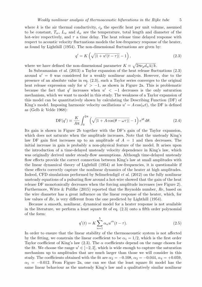
where k is the air thermal conductivity, cp the specific heat per unit volume, assumedto be constant, Tw, Lw and dw are the temperature, total length and diameter of thehot-wire respectively, and τ a time delay. The heat release time delayed response withrespect to acoustic velocity fluctuations models the low-frequency response of the heater,as found by Lighthill (1954). The non-dimensional fluctuations are given by:

q′ = K(√|1 + u′(t− τ)| − 1

), (2.3)

where we have defined the non-dimensional parameter K ≡√

2πcpdwu/k.In Subramanian et al. (2013) a Taylor expansion of the heat release fluctuations (2.3)

around u′ = 0 was considered for a weakly nonlinear analysis. However, due to thepresence of an absolute value in eq. (2.3), such a Taylor series converges to the originalheat release expression only for u′ > −1, as shown in Figure 2a. This is problematicbecause the fact that q′ increases when u′ < −1 decreases is the only saturationmechanism, which we want to model in this study. The weakness of a Taylor expansion ofthis model can be quantitatively shown by calculating the Describing Function (DF) ofKing’s model. Imposing harmonic velocity oscillations u′ = A cos(ωt), the DF is definedas (Gelb & Velde 1968):

DF(q′) ≡ K

Aπ

∫ 2π

0

(√|1 +A cos(θ − ωτ)| − 1

)eiθ dθ. (2.4)

Its gain is shown in Figure 2b together with the DF’s gain of the Taylor expansion,which does not saturate when the amplitude increases. Note that the unsteady King’slaw DF gain first increases up to an amplitude of A = 1 and then decreases. Theinitial increase in gain is probably a non-physical feature of the model. It arises uponthe introduction of a time-delayed unsteady velocity dependence in King’s law, whichwas originally derived under steady-flow assumptions. Although time-delayed unsteadyflow effects provide the correct connection between King’s law at small amplitudes withthe linear dynamical theory of Lighthill (1954) at low-frequencies, it is questionable ifthese effects correctly capture the nonlinear dynamics of the heater at high amplitudes.Indeed, CFD simulations performed by Selimefendigil et al. (2012) on the fully nonlinearunsteady equations of a pulsating flow around a hot-wire showed that the gain of the heatrelease DF monotonically decreases when the forcing amplitude increases (see Figure 2).Furthermore, Witte & Polifke (2015) reported that the Reynolds number, Re, based onthe wire diameter has a great influence on the linear response of the heater, which, forlow values of Re, is very different from the one predicted by Lighthill (1954).

Because a smooth, nonlinear, dynamical model for a heater response is not availablein the literature, we perform a least square fit of eq. (2.3) onto a fifth order polynomialof the form:

q′(t) = K

5∑n=1

αnu′n(t− τ). (2.5)

In order to ensure that the linear stability of the thermoacoustic system is not affectedby the fitting, we constrain the linear coefficient to be α1 = 1/2, which is the first orderTaylor coefficient of King’s law (2.3). The α coefficients depend on the range chosen forthe fit. We choose the range u′ ∈ [−2, 2], which is wide enough to capture the saturationmechanism up to amplitudes that are much larger than those we will consider in thisstudy. The coefficients obtained with the fit are α2 = −0.108, α3 = −0.044, α4 = +0.059,α5 = −0.012. From Figure 2a, one can see that the least square fit model has thesame linear behaviour as the unsteady King’s law and a qualitatively similar nonlinear


−2 −1 0 1 2

−1

−0.5

0

0.5

1.0

u′(t − τ)

q′(t)

0 0.5 1 1.5 20

0.1

0.2

0.3

0.4

0.5

0.6

A

|DF(q

′ )|

(a) (b)

Unsteady King’s law model

Taylor expansion

Least−square fit

CFD (Selimefendigil et al., 2012)

Figure 2. Nonlinear heat release models. (a): Comparison between unsteady King’s law, fifthorder Taylor expansion and polynomial fit approximations. K is fixed to 1. (b): The DescribingFunction gain of King’s model and its approximations. The saturation mechanism starts at A = 1and is due to the abrupt change of sign of the heat release derivative. The Taylor expansionaround u′ = 0 cannot capture this mechanism. CFD results from Selimefendigil et al. (2012)(scaled to match the linear gain) are in qualitative agreement with the least-square fit modelthat we use in this paper.

behaviour, with a smooth saturation mechanism. The saturation starts at values smallerthan u′ = 1, which is consistent with the experimental observations of Heckl (1990).Also, Figure 2b shows that the gain of the fitted model decreases monotonically withthe amplitude forcing, which is consistent with the nonlinear unsteady calculationsof Selimefendigil et al. (2012). In the following, we will find that oscillations saturatewith amplitudes |u′| < 1, for which our fit is in good agreement with CFD results. If anappropriate model for the nonlinear dynamic response of the heater is provided, the αcoefficients can be obtained via a Taylor expansion up to the desired order.

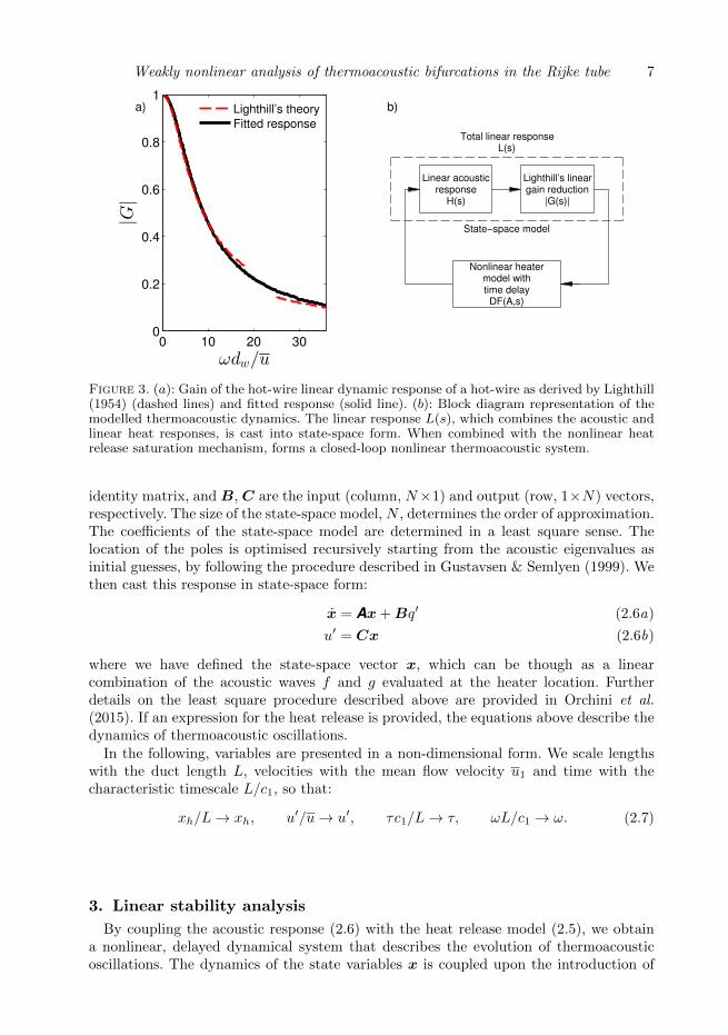
Note that the gain of (2.3) is constant for all frequencies, since it is a static heatrelease model (i.e., q′ does not depend on du′/dt). A physical mechanism that dampshigh-frequency modes has to be included, otherwise non-physical high-frequency ther-moacoustic oscillations are likely to arise. Lighthill (1954) derived analytically the lineardynamic response, G, of a hot-wire subject to velocity perturbations in the low- and high-frequency limits, showing that its behaviour is analogous to that of a low-pass filter.Lighthill’s results for the gain amplitude against frequency are reported in Figure 3a.The low-pass filter cutoff frequency is a function of the wire diameter and mean flowintensity. A gain decrease with frequency provides the necessary stabilisation of high-frequency modes. The total response of the heater is therefore given by the productbetween a linear dynamic response and a nonlinear amplitude saturation, which is aWiener-Hammerstein model. Note that here we are retaining the heater phase responsedue to the time delay in the nonlinear heating element. This is a necessary condition herefor the model to exhibit subcritical bifurcations. The latter would not be possible if thephase response had no amplitude dependence, because the gain monotonically decreaseswith the amplitude.

Lighthill’s dynamic response can be combined with the linear acoustic response H(s),by defining the total linear response L(s) ≡ H(s)|G(s)|, as shown in Figure 3b. Thus, thethermoacoustic system is modelled as a Lur’e system (a linear component in feedback loopwith a nonlinear component). We extend the linear response L to the entire Laplace spacevia the rational approximation L(s) ≈ C(sI−A)−1B, where A is a N×N matrix, I is the


0 10 20 300

0.2

0.4

0.6

0.8

1

ωdw/u

|G|

a) b)Lighthill’s theory

Fitted response

Linear acousticresponse

H(s)

Lighthill’s lineargain reduction

|G(s)|

Nonlinear heatermodel withtime delayDF(A,s)

Total linear responseL(s)

State−space model

Figure 3. (a): Gain of the hot-wire linear dynamic response of a hot-wire as derived by Lighthill(1954) (dashed lines) and fitted response (solid line). (b): Block diagram representation of themodelled thermoacoustic dynamics. The linear response L(s), which combines the acoustic andlinear heat responses, is cast into state-space form. When combined with the nonlinear heatrelease saturation mechanism, forms a closed-loop nonlinear thermoacoustic system.

identity matrix, and B, C are the input (column, N×1) and output (row, 1×N) vectors,respectively. The size of the state-space model, N , determines the order of approximation.The coefficients of the state-space model are determined in a least square sense. Thelocation of the poles is optimised recursively starting from the acoustic eigenvalues asinitial guesses, by following the procedure described in Gustavsen & Semlyen (1999). Wethen cast this response in state-space form:

x = Ax + Bq′ (2.6a)

u′ = Cx (2.6b)

where we have defined the state-space vector x, which can be though as a linearcombination of the acoustic waves f and g evaluated at the heater location. Furtherdetails on the least square procedure described above are provided in Orchini et al.(2015). If an expression for the heat release is provided, the equations above describe thedynamics of thermoacoustic oscillations.

In the following, variables are presented in a non-dimensional form. We scale lengthswith the duct length L, velocities with the mean flow velocity u1 and time with thecharacteristic timescale L/c1, so that:

xh/L→ xh, u′/u→ u′, τc1/L→ τ, ωL/c1 → ω. (2.7)

3. Linear stability analysis

By coupling the acoustic response (2.6) with the heat release model (2.5), we obtaina nonlinear, delayed dynamical system that describes the evolution of thermoacousticoscillations. The dynamics of the state variables x is coupled upon the introduction of


the heat element through the acoustic velocity u′ = Cx:

x(t) = Ax(t) +KB

5∑n=1

αn(Cx(t− τ))n (3.1)

where K is the control parameter, which determines the intensity of the heat releasefluctuations. The matrix A and the column and row vectors B and C are functions ofthe state-space model order of approximation and of the flame location xh. The latter isfixed to xh = 0.13, which is the location at which our thermoacoustic network is mostprone to thermoacoustic oscillations at its lowest eigenfrequency when the time delay ischosen to be τ = 0.04. This was obtained by searching for the maximum value of the

Rayleigh index Ry ≡∫ T0p′xh

(t)q′(t) dt, assuming harmonic oscillations and using eq. (3.1)in order to relate heat release fluctuations to velocity fluctuations.

Fixing all the other parameters, there are specific values of K, called critical points, atwhich the system is marginally stable, meaning that all the eigenvalues of the spectrumof the linear operator have a negative growth rate except for a complex conjugate pair,which has a zero growth rate. At these critical points Hopf bifurcations occur, and thelinear stability of the system changes across them. In order to perform a weakly nonlinearanalysis, we need to first locate critical points and then expand the governing equationsaround them. This will yield the amplitude and frequency of limit cycle oscillations thatoccur after the bifurcation.

The fixed point x = 0 is a solution of the dynamical system (3.1) for any value of K.Its stability is determined by the eigenvalues of the linearised system:

x(t) = Ax(t) + α1KBCx(t− τ) (3.2)

Taking the Laplace transform we have:(sI − A− α1KBCe−sτ

)x = 0 (3.3)

where s ≡ σ+iω is the non-dimensional Laplace variable, and I the identity matrix. Notethat, because B and C are column and row vectors respectively, their (outer) productresults in a matrix. The values of s for which the determinant of the linear operatorvanishes are the thermoacoustic eigenvalues. The nonlinear eigenvalue problem (3.3) issolved iteratively while varying K until a marginally stable solution is found.

We first perform a parametric study in the K − τ plane to identify a set of Hopfbifurcations of the thermoacoustic mode with the smallest eigenfrequency (see Figure 4a).This is achieved using the open-source package DDE-BIFTOOL (Engelborghs et al. 2002;Sieber et al. 2015), tracking the critical values of the heater power Kc at which the growthrate associated with the smallest eigenfrequency is zero. However, we find that, for someof these solutions, mode(s) with a higher frequency have a positive growth rate alongthe neutral lines of the first mode. This is physically possible when the values of Kc orτ are large. We show these solutions with black lines in Figure 4a. At these locationsthe system is not marginally stable, and the theory presented in the following cannotbe applied. A typical value for the time delay can be estimated from Lighthill (1954)’stheory, τ = 0.2 dw/u. For our configuration, this yields a non-dimensional value of thetime delay of order 10−2. In the following, we will fix τ = 0.04, for which the criticalpower is Kc = 1.42. Figure 4b shows the spectrum of the acoustic and thermoacousticsystems at this Hopf bifurcation.

Note that the frequencies of the thermoacousitic eigenmodes are close to the acousticones, but the growth rates are significantly shifted as K is increased. The order ofapproximation of the state-space – which is twice the number of modes considered – has to


0 0.5 1 1.5 2 2.5 30

0.1

0.2

0.3

0.4

0.5

Kc

τ

3.8

3.9

4

4.1

4.2

−0.25 −0.2 −0.15 −0.1 −0.05−50

0

50

Re(s)

Im(s)

Figure 4. (a): Neutral line in the K − τ plane. Along it, the eigenmode with the smallesteigenfrequency has zero growth rate. Colours refer to the frequency of the marginally stablemode. Black lines indicate that mode(s) with a higher frequency have a positive growth rate. (b):Spectrum of the acoustic (circles) and thermoacoustic (crosses) system for the set of parameterschosen for the weakly nonlinear analysis, marked with a circle in the left plot. The paths of theeigenvalues from their acoustic values (K = 0, dots) to their thermoacoustic values (K = Kc,crosses) are shown as dotted lines.

2 4 6 8 10 121.2

1.3

1.4

1.5

1.6

Number of modes

Kc

2 4 6 8 10 124.15

4.16

4.17

4.18

4.19

Number of modes

ωc

Figure 5. Convergence of the marginally stable angular frequency ωc (left) and critical powerKc (right) with respect to the number of modes considered in the state-space approximation.A single-mode approximation does not accurately capture the correct response of the system.

be large enough in order to capture the thermoacoustic response correctly, as was shownby Ananthkrishnan et al. (2005); Kashinath et al. (2014). A single-mode approximationof the acoustic response (as considered by Juniper (2011); Subramanian et al. (2013) forweakly nonlinear expansions) is not able to capture the system response accurately in thiscase. Figure 5 shows that the marginally stable eigenfrequency and heat power obtainedwith a single-mode approximation are different from the ones obtained with multiplemodes. The number of modes used can also affect the type of bifurcation predicted bythe weakly nonlinear expansion, as we will discuss in §4.3. In this study, we will retain 12modes when performing the weakly nonlinear analysis. Thus, our thermoacoustic systemis composed of 24 coupled differential equations. As a consequence, the use of adjointmethods is required to obtain solvability conditions of the weakly nonlinear equations,as discussed in §4.3.


4. Weakly nonlinear analysis

We now perturb the bifurcation parameter from the critical point, K = Kc+∆K, with|∆K| � 1. After the Hopf bifurcation, the system is linearly unstable and oscillationswill grow and can saturate to limit cycle oscillations due to nonlinear effects. In thecase in which the Hopf bifurcation is subcritical, a bistable region exists before the Hopfpoint in which, by triggering the system, stable solutions with a finite amplitude canbe found (Ananthkrishnan et al. 2005; Juniper 2011). To calculate the amplitude andfrequencies of these oscillations, nonlinear methods are required. We accomplish this witha weakly nonlinear analysis, by expanding the evolution of the dynamical system (3.1)around the Hopf location. We denote with 0 < ε � 1 a small quantity that quantifiesthe amplitude of the oscillations close to the Hopf point. We then seek for solutions xexpressed as power series of ε:

x = εx1 + ε2x2 + ε3x3 + ε4x4 + ε5x5 +O(ε6) (4.1)

For a subcritical bifurcation, expansion at third order yields unstable limit cycle solu-tions. However, such oscillations are typically not observable in self-excited experiments,although they can be studied experimentally by forcing the system close to the unstablesolutions (Jegadeesan & Sujith 2013). For subcritical phenomena though, one is alsointerested in calculating the amplitude of stable solutions, and to identify the width ofthe bistable region. This requires terms of at least order 5 in a weakly nonlinear expansion.

We choose to work with the method of multiple scales. With this method, one assumesthat several, independent timescales act on the system. One is the fast timescale t0, atwhich the oscillations of the marginally stable frequency respond. The slow timescalest2 and t4 are associated with long time saturation or growth processes. The total timederivative therefore reads:

d

dt=

∂

∂t0+

∂

∂t2+

∂

∂t4+ . . . (4.2)

By Taylor expanding the dynamical system (3.1) around the fixed point solution x = 0at the critical point K = Kc we obtain:

∂x

∂t0+∂x

∂t2+∂x

∂t4= Ax +

5∑n=1

αnKcB(Cx(t− τ))n . . .

+

5∑n=1

αn∆KB(Cx(t− τ))n

(4.3)

It is important to note that the orders of magnitude of O(x) = ε and those of O(∆K),O(t2), and O(t4) are not independent. Upon the expansion of the equations, one can showthat, at odd orders larger than 1, secular terms (i.e., forcings at resonant frequencies)arise due to nonlinear interactions. Solvability conditions need to be imposed on theseforcings, which have to be balanced by contributions arising from slow timescales andcontrol parameter terms (Rosales 2004; Strogatz 2015). This reasoning leads to balancesbetween the order of magnitudes of the various terms, which read:

O(x∆K) = ε3, O(∂x

∂t2

)= ε3, O

(∂x

∂t4

)= ε5 (4.4)

We shall then rewrite all the quantities in terms of ε by defining ∆K ≡ ε2δ2, t2 ≡ ε2t2and t4 ≡ ε4t4. The parameter δ2 can take the values ±1 depending on the side of theHopf point we are investigating. From the definition of ∆K, we also obtain a measure of


the expansion parameter in terms of the distance from the Hopf location:

ε =√|K −Kc| (4.5)

Note that ε needs to be � 1. In the following, we will show that the largest value ofthe bifurcation parameter we need to consider to locate the fold point of a subcriticalbifurcation is ε ≈ 0.05, which satisfies this condition.

Lastly, the time delay contained in our system acts at all the timescales we areconsidering (Das & Chatterjee 2002). Considering the ε scalings just discussed for theslow timescales, delayed variables are therefore functions of t0− τ , t2− ε2τ , and t4− ε4τ .These terms are then expanded in series of ε. For ease of notation, in the following wewill adopt the short notation x(t) for x(t0, t2, t4), and x(t− τ) for x(t0 − τ, t2, t4).

We now substitute the relations (4.1), (4.4) into eq. (4.3). The complete list of terms weobtain is given in Appendix B. By matching these terms by their ε order, we obtain a set oflinear, inhomogeneous differential equations which have to be solved in ascending order.We perform the weakly nonlinear expansion up to O(ε5); in the following subsections wewill solve and discuss the equations order by order.

4.1. O(ε): eigenvalue problem

At order ε we retrieve the homogeneous linear eqs. (4.6) for the evolution of x1:

∂x1

∂t0− Ax1 − α1K

cB(Cx1(t− τ)) = 0. (4.6)

Because the left hand structure of the equations will be the same at all ε orders, it isconvenient to define the spectral operator:

Ms ≡(sI − A− α1K

cBCe−sτ), (4.7)

so that the nonlinear eigenvalue problem in the frequency domain can be rewritten asMsx1 = 0. This is the same eigenvalue problem as in eq. (3.3). Also, because here wehave fixed K = Kc, we know that the system is marginally stable (its spectrum is shownin Figure 4b with crosses).

We can simplify the evolution of the dynamical system to the evolution of themarginally stable thermoacoustic eigenmode only, i.e., by ignoring the contribution ofthe eigenmodes with a negative growth rate, because they will quickly be damped (Sipp& Lebedev 2007). Close to the Hopf bifurcation, we expect the dynamical system tosaturate to limit cycle oscillations at the slow timescales, therefore we can write:

x1 ≈W (t2, t4)xW1 eiωct0 + c.c., (4.8)

where ωc is the angular frequency of the marginally stable eigenmode, xW1 the correspond-ing right eigenvector and W (t2, t4) a complex valued variable which depends on the slowtimescales only. W contains information on the amplitude saturation and frequency shifteffects caused by nonlinear effects. At the next odd orders, we will explicitly find thedependence of W with respect to the slow timescales.

4.2. O(ε2): mean shift and second harmonic

At this order we obtain the equations for the evolution of x2. From this order on,forcing terms will appear in the r.h.s. of the equations. In general, the forcing terms atorder εN are due to the nonlinear interactions between the solutions xk at orders k < N ,which are known. The only forcing term at this order is α2K

cB(Cx1(t− τ))2, which isdue to the interaction of x1 with itself. By using the expression (4.8) for x1, we obtain


the inhomogeneous linear equation:

∂x2

∂t0− Ax2 − α1K

cB(Cx2(t− τ)) = |W |2F |W |2

2 +(W 2FW 2

2 e2iωct0 + c.c.

), (4.9)

where

FW 2

2 ≡ α2KcB(CxW1 )2e−2iω

cτ ,

F|W |22 ≡ 2α2K

cB|CxW1 |2.(4.10)

The superscripts are used to classify the forcing terms by their dependence on thecomplex amplitudes W . This forcing is composed of two components: a steady forcingwith zero frequency (due to the interaction between the eigenmode xW1 and its complexconjugate), and second harmonic contributions at frequency 2ωc (due to the interactionbetween the eigenmode xW1 and itself). These are not resonant terms, because thespectrum of the linear operator does not contain 2ωc or 0 as eigenvalues (see Figure 4b),and eqs. (4.9) can be readily solved.

We look for a steady-state solution x2 which has the same shape as the forcing, byusing the ansatz

x2 = |W |2x|W |2

2 +(W 2xW

2

2 e2iωct0 + c.c.

). (4.11)

Substituting the latter into eq. (4.9), taking the Laplace transform (with respect to thefast timescale t0), and matching the terms according to their amplitude dependence, weobtain the sets of linear equations:

M2iωcxW2

2 = FW 2

2 , (4.12a)

M0x|W |22 = F

|W |22 . (4.12b)

The matrices M2iωc and M0 are non-singular and can be inverted, yielding the solutionsat the various amplitude levels of x2.

In particular, xW2

2 (and its c.c.) describes second harmonic oscillations, whereas x|W |22 ,

having zero frequency, will cause a shift in the mean acoustic level, caused by the presenceof even terms in the expansion of the nonlinear heater element response. This is a well-known effect in hydrodynamics, where zero frequency corrections are due to quadraticterms arising from the nonlinear convective term of the Navier–Stokes equations. Aweakly nonlinear expansion allows distinction between the base flow (solution of thesteady Navier–Stokes equations) and the mean flow (time averaged solution of theunsteady Navier–Stokes equations) (Sipp & Lebedev 2007; Meliga et al. 2009). Theseeffects are not found if the nonlinearity expansion contains only odd terms. This is oftenthe case for low-order thermoacoustic modelling (Noiray et al. 2011; Noiray & Schuermans2013; Ghirardo et al. 2015), although some experimental evidence of acoustic level meanshifts can be found in the literature (Flandro et al. 2007).

4.3. O(ε3): third harmonic and saturation

At this order we obtain the equations for the evolution of x3:

∂x3

∂t0− Ax3 − α1K

cB(Cx3(t− τ)) = −∂x1

∂t2− τBα1K

cC∂x1

∂t2(t− τ) . . .

+(WFW

3 eiωct0 + |W |2WF

|W |2W3 eiω

ct0 +W 3FW 3

3 e3iωct0 + c.c.

) (4.13)


The explicit expressions of the forcing terms are reported in Appendix C.1. The slowtimescales’ derivatives may be rewritten as:

∂x1

∂t2(t) =

∂W

∂t2xW1 eiω

ct + c.c.. (4.14)

Resonant forcings arise at this order, with angular frequency ωc, which act on twodifferent amplitude levels, W and |W |2W . A solvability condition, known as the Fredholmalternative (Oden & Demkowicz 2010), needs to be satisfied for a solution to exist. Itrequires the sum of the resonant forcing terms to be orthogonal to the kernel (nullspace)

of the (singular) adjoint operator M†iωc (Sipp & Lebedev 2007; Meliga et al. 2009). Thisgeneralises the idea of cancelling the secular terms used for weakly nonlinear analysis ofscalar problems.

The adjoint matrix Miωc is defined through the scalar product:⟨y,Miωcx

⟩=⟨

M†iωcy,x⟩

(4.15)

and corresponds to the Hermitian of the direct matrix Miωc . The latter has a zeroeigenvalue, which corresponds to the direct eigenvector xW

1 . Because an adjoint matrix

has eigenvalues which are complex conjugate of those of its direct matrix, M†iωc has a

zero eigenvalue, and its kernel is spanned by the adjoint eigenvector x†1 only. This canbe calculated as the Hermitian of the left eigenvector of the operator Miωc correspondingto the eigenvalue 0. The solvability condition therefore requires:⟨

x†1,−∂W

∂t2PxW1 +WFW

3 + |W |2WF|W |2W3

⟩= 0, (4.16)

where the right terms in the bracket are all the resonant forcings, and we have definedthe matrix P ≡

(I + τBα1K

cCe−iωcτ). By rearranging eq. (4.16), we obtain:

∂W

∂t2= λ3W + ν3|W |2W (4.17)

where the complex values λ3, ν3, known as the Landau coefficients, are defined by:

λ3 ≡

⟨x†1,F

W3

⟩⟨x†1,PxW1

⟩ , ν3 ≡

⟨x†1,F

|W |2W3

⟩⟨x†1,PxW1

⟩ . (4.18)

The values we found for the Landau coefficients when K < Kc are λ3 = −0.0659−0.1523iand ν3 = 0.0007− 0.0048i. The dependence of the Landau coefficients on the number ofmodes retained in the acoustic state-space model is shown in Figure 6a. Note that, inthis case, we find that the sign of Re(ν3) with one mode is different from the sign of thesaturated value, containing multiple modes, whereas the sign of Re(λ3) does not change.The sign of the ratio of the latter values is important, as it distinguishes between sub- andsupercritical bifurcations. This shows that the nature of the bifurcation predicted witha single mode approximation may be different from the actual response of the system.

We then seek a solution x3 via the ansatz:

x3 = WxW3 eiωct0 + |W |2Wx

|W |2W3 eiω

ct0 +W 3xW3

3 e3iωct0 + c.c. (4.19)

By using the relation (4.17), we match the solution and forcing terms of (4.13) by their


dependence on the amplitude W , and obtain the sets of linear equations:

MiωcxW3 = FW3 − λ3PxW1 , (4.20a)

Miωcx|W |2W3 = F

|W |2W3 − ν3PxW1 , (4.20b)

M3iωcxW3

3 = FW 3

3 . (4.20c)

Although the matrix Miωc is singular, the values of the Landau coefficients guarantee that

solutions for xW3 and x|W |2W3 exist. They can be calculated, e.g., by using the pseudo-

inverse matrix of Miωc . These solutions provide a nonlinear correction to the shape ofthe linearly unstable mode. Eq. (4.20c), instead, can be readily solved by inverting the

matrix M3iωc , which is non-singular. xW3

3 accounts for third harmonic contributions tothe oscillatory solution.

4.3.1. Stuart–Landau equation: O(ε3)

Equation (4.17) is known as the Stuart–Landau equation. Its roots yield the amplitudeof limit cycle solutions and the frequency shift of the nonlinear oscillation with respect tothe marginally stable eigenfrequency. By using the polar representation W = reiθ, andby splitting the real and the imaginary parts, we have:

∂r

∂t2= Re(λ3)r + Re(ν3)r3, (4.21a)

∂θ

∂t2= Im(λ3) + Im(ν3)r2. (4.21b)

The equation for the phase θ is valid only for solutions with non-zero amplitude. Steady-state solutions are reached when the amplitude r does not vary in time. The amplitudelevels at which this happens are:

r1 = 0, r2 =

√−Re(λ3)

Re(ν3). (4.22)

From the definitions (4.18), (C 2a), one can see that λ3, being proportional to δ2 = ±1,changes sign across the critical point Kc, whereas ν3 does not vary when we change thebifurcation parameter. Therefore, the solution r2 is real only on one side of the Hopflocation. The stability of the solutions is connected to the sign of the eigenvalue of theJacobian J ≡ Re(λ3) + 3Re(ν3)r2 evaluated at the two solutions. These values are:

J(r1) = Re(λ3), J(r2) = −2Re(λ3). (4.23)

Note that, in the region where two solutions coexist, their stability is different. Thisdistinguishes between super- and subcritical Hopf bifurcations. For the set of parameterswe have chosen, we find that the bifurcation is subcritical: before the Hopf bifurcation,stable fixed points and unstable limit cycle solutions exist, and after it only unstablefixed point solutions are found, as shown in Figure 6b. The present analysis could be alsoapplied to configurations in which the bifurcation is supercritical.

The solution of the phase equation (4.21b) on the unstable limit cycle solution reads:

θ = ε2(

Im(λ3)− Im(ν3)Re(λ3)

Re(ν3)

)t0 ≡ ∆ωt0, (4.24)

where we have used the scaling t2 = ε2t0 between the fast and slow timescales. ∆ωrepresents the frequency shift between the fundamental oscillation frequency of limitcycles and the marginally stable frequency ωc.


1 2 3 4 5 6 7 8 9 10 11 12−10

−5

0

5x 10

−3

Number of modes

1 2 3 4 5 6 7 8 9 10 11 120

0.1

0.2Landau C

oeffic

ients

Re(λ3) Im(λ

3) Re(ν

3) Im(ν

3)

1.41 1.42 1.43 1.440

0.2

0.4

0.6

0.8

1

K

|u′ iω|

Kc

Third order subcriticalbifurcation diagram

Figure 6. (a): Saturation of the Landau coefficients λ3, ν3 with respect to the number ofmodes. (b): Subcritical Hopf bifurcation diagram. Solid and dashed lines represent stable andunstable solutions, respectively. The oscillation’s amplitude at the fundamental frequency withcorrections up to ε3 is shown.

Combining the power expansion (4.1), the weakly nonlinear solutions (4.8), (4.11),(4.19) and the solution of the Stuart–Landau equation, we obtain an analytical expressionfor the time evolution of the thermoacoustic states up to third order, which reads:

x = ε2r2x|W |22 +

[εrxW1 + ε3rxW3 + ε3r3x

|W |2W3

]ei(ω

c+∆ω)t0 . . .

+ε2r2xW2

2 e2i(ωc+∆ω)t0 + ε3r3xW

3

3 e3i(ωc+∆ω)t0 + c.c. +O(ε4).

(4.25)

Figure 6b shows the subcritical bifurcation diagram we obtain at this order. It containsthe amplitude level of the velocity fluctuations u′ = Cx calculated from eq. (4.25)at the fundamental frequency. We shall postpone the discussion of the response atother frequencies to section §5. Because these limit cycle oscillations are unstable,the amplitudes that the Stuart–Landau equation predicts at this order correspondapproximately to the level of triggering which is required to excite finite amplitudeoscillations. In order to predict the amplitude of stable limit cycles, we need to extendthe weakly nonlinear expansion to higher orders.

4.4. O(ε4): mean shift and fourth harmonic

At this order we obtain the equations for the evolution of x4:

∂x4

∂t0− Ax4 − α1KB(Cx4(t− τ)) = |W |4F |W |

4

4 + |W |2F |W |2

4 . . .

+(W 2FW 2

4 e2iωct0 + |W |2W 2F

|W |2W 2

4 e2iωct0 +W 4FW 4

4 e4iωct0 + c.c

).

(4.26)

None of the forcing terms resonates. Their expressions are provided in Appendix C.2.Using the ansatz:

x4 = |W |2x|W |2

4 + |W |4x|W |4

4 . . .

+(W 2xW

2

4 e2iωct0 + |W |2W 2x

|W |2W 2

4 e2iωct0 +W 4xW

4

4 e4iωct0 + c.c.

),

(4.27)


we can readily calculate the solutions

x|W |24 = M−10 F

|W |24 (4.28a)

x|W |44 = M−10 F

|W |44 (4.28b)

xW2

4 = M−12iωcFW 2

4 (4.28c)

x|W |2W 2

4 = M−12iωcF|W |2W 2

4 (4.28d)

xW4

4 = M−14iωcFW 4

4 (4.28e)

which provide contributions to the mean acoustic level shift, and second and fourthharmonic oscillations.

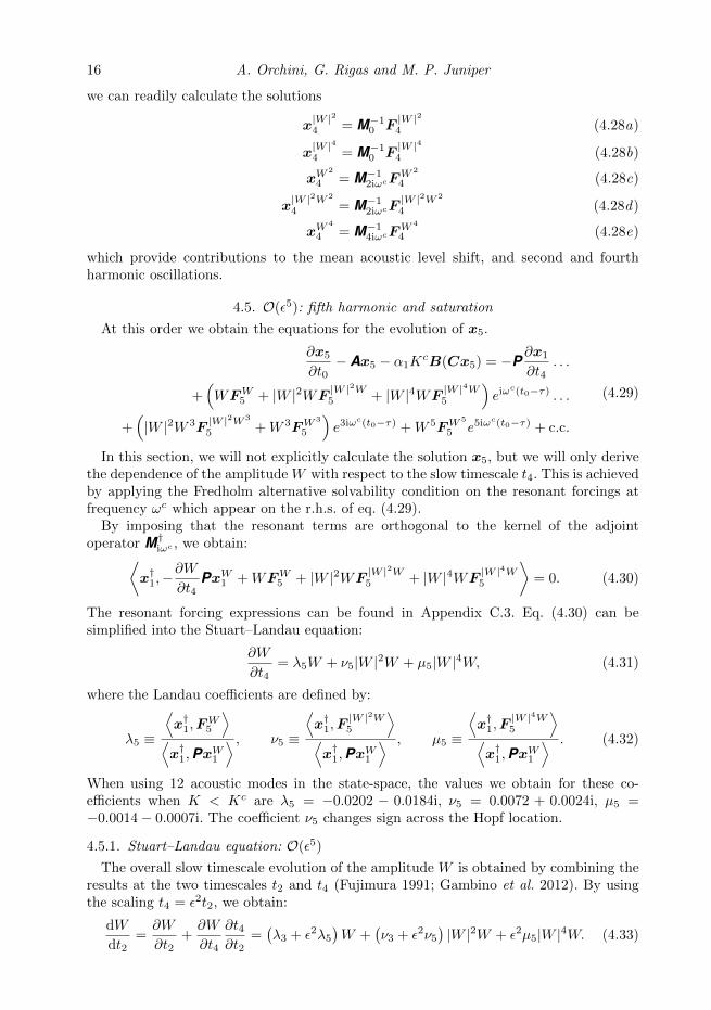
4.5. O(ε5): fifth harmonic and saturation

At this order we obtain the equations for the evolution of x5.

∂x5

∂t0− Ax5 − α1K

cB(Cx5) = −P∂x1

∂t4. . .

+(WFW

5 + |W |2WF|W |2W5 + |W |4WF

|W |4W5

)eiω

c(t0−τ) . . .

+(|W |2W 3F

|W |2W 3

5 +W 3FW 3

5

)e3iω

c(t0−τ) +W 5FW 5

5 e5iωc(t0−τ) + c.c.

(4.29)

In this section, we will not explicitly calculate the solution x5, but we will only derivethe dependence of the amplitude W with respect to the slow timescale t4. This is achievedby applying the Fredholm alternative solvability condition on the resonant forcings atfrequency ωc which appear on the r.h.s. of eq. (4.29).

By imposing that the resonant terms are orthogonal to the kernel of the adjointoperator M†iωc , we obtain:⟨

x†1,−∂W

∂t4PxW1 +WFW

5 + |W |2WF|W |2W5 + |W |4WF

|W |4W5

⟩= 0. (4.30)

The resonant forcing expressions can be found in Appendix C.3. Eq. (4.30) can besimplified into the Stuart–Landau equation:

∂W

∂t4= λ5W + ν5|W |2W + µ5|W |4W, (4.31)

where the Landau coefficients are defined by:

λ5 ≡

⟨x†1,F

W5

⟩⟨x†1,PxW1

⟩ , ν5 ≡

⟨x†1,F

|W |2W5

⟩⟨x†1,PxW1

⟩ , µ5 ≡

⟨x†1,F

|W |4W5

⟩⟨x†1,PxW1

⟩ . (4.32)

When using 12 acoustic modes in the state-space, the values we obtain for these co-efficients when K < Kc are λ5 = −0.0202 − 0.0184i, ν5 = 0.0072 + 0.0024i, µ5 =−0.0014− 0.0007i. The coefficient ν5 changes sign across the Hopf location.

4.5.1. Stuart–Landau equation: O(ε5)

The overall slow timescale evolution of the amplitude W is obtained by combining theresults at the two timescales t2 and t4 (Fujimura 1991; Gambino et al. 2012). By usingthe scaling t4 = ε2t2, we obtain:

dW

dt2=∂W

∂t2+∂W

∂t4

∂t4∂t2

=(λ3 + ε2λ5

)W +

(ν3 + ε2ν5

)|W |2W + ε2µ5|W |4W. (4.33)


1.42 1.422 1.4240

0.1

0.2

0.3

0.4

0.5

0.6

K

|u′ iω|

Kc

KF

O(ǫ3)O(ǫ5)

Figure 7. Comparison between third order (black) and fifth order (red) bifurcation diagrams.The analytically calculated amplitude of the acoustic velocity at the fundamental frequency isshown, according to (4.25). At fifth order the limit cycle saturates, so the limit cycle amplitudeand the location of the fold point KF can be calculated.

By using the polar representation W = reiθ, this decouples into:

dr

dt2= Re(λ)r + Re(ν)r3 + Re(µ)r5, (4.34a)

dθ

dt2= Im(λ) + Im(ν)r2 + Im(µ)r4, (4.34b)

where λ = λ3+ε2λ5, and similarly for ν and µ. The fixed points of the amplitude equationare:

r1 = 0, r2,3 =

√−Re(ν)±

√(Re(ν))2 − 4Re(λ)Re(µ)

2Re(µ). (4.35)

The existence of real solutions for r2,3 depends only on the sign of the terms under thesquare roots. Because the bifurcation is subcritical, we have two solutions after the Hopflocation (an unstable fixed point and a stable limit cycle), a bistable region between theHopf and the fold points with three solutions (a stable fixed point, an unstable and astable limit cycle), and a region with only one stable fixed point before the fold. This isshown in Figure 7, where the path that the oscillations will follow when the bifurcationparameter is varied across the bistable region is shown with arrows. As expected, closeto the Hopf point the fifth order expansion correctly matches the third order analysis.

The stability of the solutions is determined by the sign of the Jacobian J = Re(λ) +3Re(ν)r2 + 5Re(µ)r4 evaluated at the solutions. These values are:

J(r1) = Re(λ), (4.36a)

J(r2,3) = −4Re(λ) +(Re(ν))2

Re(µ)∓ Re(ν)

√(Re(ν))2 − 4Re(λ)Re(µ). (4.36b)

The frequency shift ∆ω on the limit cycles can be readily calculated from eq. (4.34b)by using the scaling t2 = ε2t0:

∆ω2,3 ≡ ε2(Im(λ) + Im(ν)r22,3 + Im(µ)r42,3

)(4.37)


0.000 0.500 1.000 1.319 1.320

−0.8

−0.6

−0.4

−0.2

0

0.2

0.4

0.6

0.8

t

u′

5000 6000 700010

−2

10−1

100

σ =4.700e-04

×104

2 4 6 8 10

x 104

−0.4

−0.3

−0.2

−0.1

0

0.1

0.2

0.3

t

u′

5 6 7

x 104

10−3

10−2

10−1

σ =-1.067e-04

Figure 8. a): at K = Kc+∆K = 1.43 the fixed point solution becomes unstable and oscillationsgrow to a limit cycle. b): at K = 1.421 no limit cycle solutions exist, and the system convergesto fixed point solutions even when initialised to a highly perturbed state. The insets showthe exponential growth and decay rates of the oscillations in a logarithmic scale. The growthrate is extracted by performing a fit (red line in the insets) onto the magnitude of the Hilberttransformed signal.

5. Results validation

We now compare the weakly nonlinear analysis discussed in §4 with the fully-nonlinearresults obtained by solving the nonlinear dynamical system (3.1) with no approximations.This is achieved with two methods: time marching the governing equations, and numericalcontinuation of limit cycles. Time domain simulations are performed using MATLABdelay differential equations solver dde23, and the numerical continuation algorithm isbased on the DDE-BIFTOOL package (Engelborghs et al. 2002). Although the lattercan only predict periodic oscillations and their stability, we find that, for the set ofparameters we have investigated, the system always converges towards fixed points orperiodic oscillations. Therefore, the two methods yield the same results for the steady-state response, as it was verified.

5.1. Time domain simulations

Time domain simulations are performed by initialising the integration to a state whichis slightly perturbed from the fixed point solution. Because the equations are timedelayed, the initial state covers the history of the system for a time −τ 6 t 6 0. Westart from a value of K < Kc, and then increase it in steps of ∆K. Until K 6 Kc, theinitial perturbations are damped and the system converges to fixed points solutions. AtK = 1.43, the oscillations start growing and converge towards a limit cycle attractorwith a large amplitude (see Figure 8a). This solution is used to initialise the subsequentintegrations, for which the control parameter K is varied in both directions in steps of±∆K. The amplitude of the oscillations gets larger as K increases. On the other hand,the amplitude of the velocity fluctuations decreases smoothly for K < Kc, until we reachthe fold location at KF = 1.421. At this location, the initialised highly perturbed initialstate decays to the fixed point solution, as shown in Figure 8b. The largest value of thecontrol parameter we consider is Kmax = 1.424, for which the parameter expansion ofthe weakly nonlinear analysis is εmax =

√Kmax −Kc = 0.039� 1.

To validate the linear analysis, the growth/decay rates close to the Hopf/fold locationsare extracted from the time series by using linear regression on the logarithm of thefluctuations amplitude. The latter is obtained using the Hilbert transform intervals ofthe time series, corresponding to the linear amplitude regime. The growth and decayrates, reported in Figure 8, can be compared with those we obtain when solving the


1.421 1.422 1.423 1.4240

0.1

0.2

0.3

0.4

0.5

K

|u′ iω|

Kc

KF

1.421 1.422 1.423 1.424−0.003

−0.002

−0.001

0

K∆ω

Kc

KF

O(ǫ3) O(ǫ5) Numerical continuation

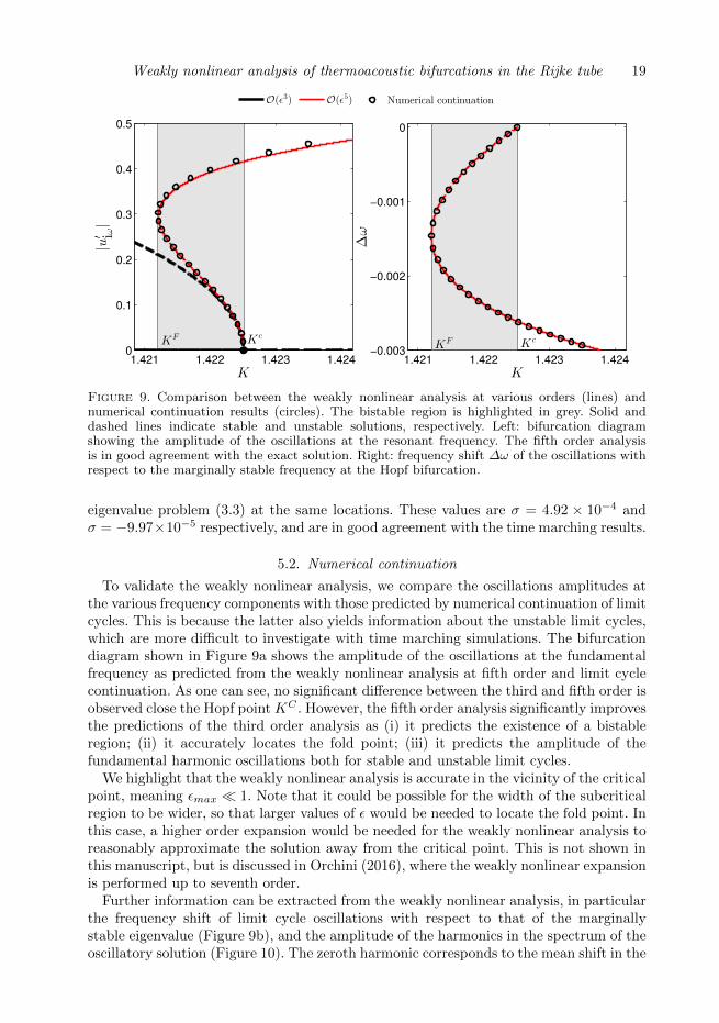
Figure 9. Comparison between the weakly nonlinear analysis at various orders (lines) andnumerical continuation results (circles). The bistable region is highlighted in grey. Solid anddashed lines indicate stable and unstable solutions, respectively. Left: bifurcation diagramshowing the amplitude of the oscillations at the resonant frequency. The fifth order analysisis in good agreement with the exact solution. Right: frequency shift ∆ω of the oscillations withrespect to the marginally stable frequency at the Hopf bifurcation.

eigenvalue problem (3.3) at the same locations. These values are σ = 4.92 × 10−4 andσ = −9.97×10−5 respectively, and are in good agreement with the time marching results.

5.2. Numerical continuation

To validate the weakly nonlinear analysis, we compare the oscillations amplitudes atthe various frequency components with those predicted by numerical continuation of limitcycles. This is because the latter also yields information about the unstable limit cycles,which are more difficult to investigate with time marching simulations. The bifurcationdiagram shown in Figure 9a shows the amplitude of the oscillations at the fundamentalfrequency as predicted from the weakly nonlinear analysis at fifth order and limit cyclecontinuation. As one can see, no significant difference between the third and fifth order isobserved close the Hopf point KC . However, the fifth order analysis significantly improvesthe predictions of the third order analysis as (i) it predicts the existence of a bistableregion; (ii) it accurately locates the fold point; (iii) it predicts the amplitude of thefundamental harmonic oscillations both for stable and unstable limit cycles.

We highlight that the weakly nonlinear analysis is accurate in the vicinity of the criticalpoint, meaning εmax � 1. Note that it could be possible for the width of the subcriticalregion to be wider, so that larger values of ε would be needed to locate the fold point. Inthis case, a higher order expansion would be needed for the weakly nonlinear analysis toreasonably approximate the solution away from the critical point. This is not shown inthis manuscript, but is discussed in Orchini (2016), where the weakly nonlinear expansionis performed up to seventh order.

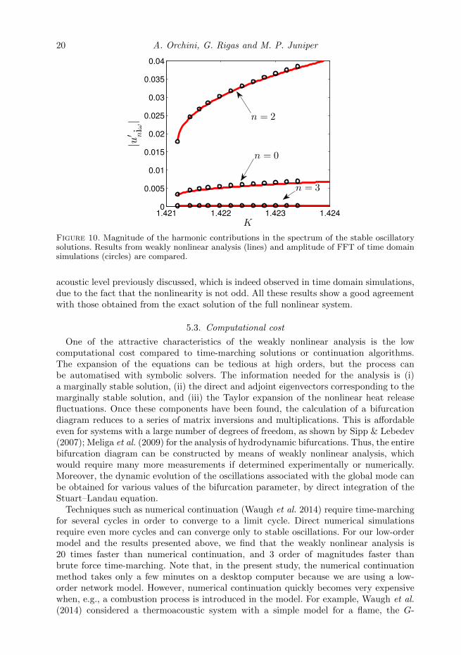
Further information can be extracted from the weakly nonlinear analysis, in particularthe frequency shift of limit cycle oscillations with respect to that of the marginallystable eigenvalue (Figure 9b), and the amplitude of the harmonics in the spectrum of theoscillatory solution (Figure 10). The zeroth harmonic corresponds to the mean shift in the


1.421 1.422 1.423 1.4240

0.005

0.01

0.015

0.02

0.025

0.03

0.035

0.04

K

|u′ niω| n = 2

n = 0

n = 3

Figure 10. Magnitude of the harmonic contributions in the spectrum of the stable oscillatorysolutions. Results from weakly nonlinear analysis (lines) and amplitude of FFT of time domainsimulations (circles) are compared.

acoustic level previously discussed, which is indeed observed in time domain simulations,due to the fact that the nonlinearity is not odd. All these results show a good agreementwith those obtained from the exact solution of the full nonlinear system.

5.3. Computational cost

One of the attractive characteristics of the weakly nonlinear analysis is the lowcomputational cost compared to time-marching solutions or continuation algorithms.The expansion of the equations can be tedious at high orders, but the process canbe automatised with symbolic solvers. The information needed for the analysis is (i)a marginally stable solution, (ii) the direct and adjoint eigenvectors corresponding to themarginally stable solution, and (iii) the Taylor expansion of the nonlinear heat releasefluctuations. Once these components have been found, the calculation of a bifurcationdiagram reduces to a series of matrix inversions and multiplications. This is affordableeven for systems with a large number of degrees of freedom, as shown by Sipp & Lebedev(2007); Meliga et al. (2009) for the analysis of hydrodynamic bifurcations. Thus, the entirebifurcation diagram can be constructed by means of weakly nonlinear analysis, whichwould require many more measurements if determined experimentally or numerically.Moreover, the dynamic evolution of the oscillations associated with the global mode canbe obtained for various values of the bifurcation parameter, by direct integration of theStuart–Landau equation.

Techniques such as numerical continuation (Waugh et al. 2014) require time-marchingfor several cycles in order to converge to a limit cycle. Direct numerical simulationsrequire even more cycles and can converge only to stable oscillations. For our low-ordermodel and the results presented above, we find that the weakly nonlinear analysis is20 times faster than numerical continuation, and 3 order of magnitudes faster thanbrute force time-marching. Note that, in the present study, the numerical continuationmethod takes only a few minutes on a desktop computer because we are using a low-order network model. However, numerical continuation quickly becomes very expensivewhen, e.g., a combustion process is introduced in the model. For example, Waugh et al.(2014) considered a thermoacoustic system with a simple model for a flame, the G-


equation. It required 14 000 CPU hours to build a bifurcation diagram with numericalcontinuation. Using weakly nonlinear analysis, one only has to calculate the direct andadjoint eigenstates around the Hopf point, and perform a small number of matrixinversions (10 matrix inversions were needed for the analysis presented here). Theseoperations can be expensive as well for systems with many degrees of freedom, but thisis affordable nowadays (Sipp & Lebedev 2007) and it is much cheaper than any methodinvolving time marching of the equations.

6. Conclusions

In this study we have investigated nonlinear thermoacoustic oscillations in a Rijketube using a fifth order weakly nonlinear expansion of the governing equations. Theframework we analysed, composed of a wave-based approach for the linear acousticequations and a nonlinear model for the heat release response, is general and can beextended to more complex networks. We have shown how a weakly nonlinear expansionclose to the Hopf bifurcations can be used to predict the amplitude and frequency ofstable and unstable limit cycles and the region of bistability for subcritical bifurcations.We have compared our weakly nonlinear results with those obtained by time-marchingthe fully-nonlinear thermoacoustic equations, which does not introduce any furtherapproximation in the governing equations, and we have shown that the method yieldsaccurate results when the expansion is truncated at fifth order. Using this type of analysis,the numerical/experimental effort needed to construct a bifurcation diagram can besignificantly reduced.

The method requires an analytical model for the description of the nonlinear heatrelease dynamics. It can be challenging, however, to obtain such a model when, say, thedynamics of a turbulent flame is considered. To overcome this issue, nonlinear systemidentification procedures could be used to fit the α coefficients of the weakly nonlinearresponse onto the flame nonlinear response (measured with a series of experiments).The latter procedure can be performed only around frequencies at which thermoacousticinstabilities are expected. The latter can be easily determined via a network model ifFlame Transfer Function (FTF) measurements are available. All the information requiredfor the weakly nonlinear analysis is then known and the theory can be applied.

The weakly nonlinear analysis we performed is valid for a deterministic system, close toa Hopf bifurcation, and assumes that only one thermoacoustic mode is marginally stableand all the others are damped. The influence of turbulence and combustion noise canbe modelled phenomenologically as random forcing (Noiray & Schuermans 2013; Rigaset al. 2015b), the effects of which can be captured by including stochastic forcing in theStuart–Landau equation. In certain problems, a second mode may become marginallystable in the vicinity of the first Hopf location. In this case, the theory can be extendedby considering a codimension two bifurcation, as described in Meliga et al. (2009). It canalso be extended to investigate the response of the system to external unsteady or steadyforcing. In this case, the forcing terms appear explicitly in the amplitude equations, asshown by Sipp (2012), and the weakly nonlinear interaction between the global mode andthe forcing is taken explicitly into account. Moreover, the unknown Landau coefficientsof the model can be identified from transient and steady-state measurements when thesystem is subjected to external forcing (Rigas et al. 2016) even for turbulent cases. Thismethod could provide a systematic way for devising open-loop control strategies for theregulation of thermoacoustic oscillations (Paschereit & Gutmark 2008; Cosic et al. 2012).


This study was founded by the European Research Council through project ALORS2590620.

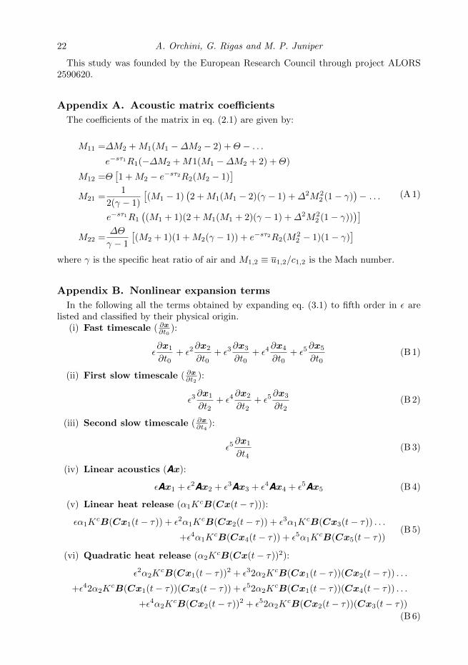
Appendix A. Acoustic matrix coefficients

The coefficients of the matrix in eq. (2.1) are given by:

M11 =∆M2 +M1(M1 −∆M2 − 2) +Θ − . . .e−sτ1R1(−∆M2 +M1(M1 −∆M2 + 2) +Θ)

M12 =Θ[1 +M2 − e−sτ2R2(M2 − 1)

]M21 =

1

2(γ − 1)

[(M1 − 1)

(2 +M1(M1 − 2)(γ − 1) +∆2M2

2 (1− γ))− . . .

e−sτ1R1

((M1 + 1)(2 +M1(M1 + 2)(γ − 1) +∆2M2

2 (1− γ)))]

M22 =∆Θ

γ − 1

[(M2 + 1)(1 +M2(γ − 1)) + e−sτ2R2(M2

2 − 1)(1− γ)]

(A 1)

where γ is the specific heat ratio of air and M1,2 ≡ u1,2/c1,2 is the Mach number.

Appendix B. Nonlinear expansion terms

In the following all the terms obtained by expanding eq. (3.1) to fifth order in ε arelisted and classified by their physical origin.

(i) Fast timescale ( ∂x∂t0 ):

ε∂x1

∂t0+ ε2

∂x2

∂t0+ ε3

∂x3

∂t0+ ε4

∂x4

∂t0+ ε5

∂x5

∂t0(B 1)

(ii) First slow timescale ( ∂x∂t2 ):

ε3∂x1

∂t2+ ε4

∂x2

∂t2+ ε5

∂x3

∂t2(B 2)

(iii) Second slow timescale ( ∂x∂t4 ):

ε5∂x1

∂t4(B 3)

(iv) Linear acoustics (Ax):

εAx1 + ε2Ax2 + ε3Ax3 + ε4Ax4 + ε5Ax5 (B 4)

(v) Linear heat release (α1KcB(Cx(t− τ))):

εα1KcB(Cx1(t− τ)) + ε2α1K

cB(Cx2(t− τ)) + ε3α1KcB(Cx3(t− τ)) . . .

+ε4α1KcB(Cx4(t− τ)) + ε5α1K

cB(Cx5(t− τ))(B 5)

(vi) Quadratic heat release (α2KcB(Cx(t− τ))2):

ε2α2KcB(Cx1(t− τ))2 + ε32α2K

cB(Cx1(t− τ))(Cx2(t− τ)) . . .

+ε42α2KcB(Cx1(t− τ))(Cx3(t− τ)) + ε52α2K

cB(Cx1(t− τ))(Cx4(t− τ)) . . .

+ε4α2KcB(Cx2(t− τ))2 + ε52α2K

cB(Cx2(t− τ))(Cx3(t− τ))

(B 6)


(vii) Linear heat release and ∆K coupling (α1δ2B(Cx(t− τ))):

ε3α1δ2B(Cx1(t− τ)) + ε4α1δ2B(Cx2(t− τ)) + ε5α1δ2B(Cx3(t− τ)) (B 7)

(viii) Cubic heat release (α3KcB(Cx(t− τ))3):


cB(Cx1(t− τ))2(Cx2(t− τ)) . . .

+ε53α3KcB(Cx1(t− τ))2(Cx3(t− τ)) + ε53α3K

cB(Cx1(t− τ))(Cx2(t− τ))2(B 8)

(ix) Quadratic heat release and ∆K coupling (α2δ2B(Cx(t− τ))2):

ε4α2δ2B(Cx1(t− τ))2 + ε52α2δ2B(Cx1(t− τ))(Cx2(t− τ)) (B 9)

(x) Quartic heat release (α4KcB(Cx(t− τ))4):


cB(Cx1(t− τ))3(Cx2(t− τ)) (B 10)

(xi) Cubic heat release and ∆K coupling (α3δ2B(Cx(t− τ))3):

ε5α3δ2B(Cx1(t− τ))3 (B 11)

(xii) Quintic heat release (α5KcB(Cx(t− τ))5):

ε5α5KcB(Cx1(t− τ))5 (B 12)

(xiii) Time delay (proportional to τ , τ2)

−τBα1KcC

∂x1

∂t2(t− τ)ε3 . . .

+τB

(−2α2K

cCx1(t− τ)C∂x1

∂t2(t− τ)− α1K

cC∂x2

∂t2(t− τ)

)ε4 . . .

+τB

[−α1K

cC∂x1

∂t4(t− τ)− α1δ2C

∂x1

∂t2(t− τ) . . .

−3α3Kc(Cx1(t− τ))2C

∂x1

∂t2(t− τ)− 2α2K

cCx2(t− τ)C∂x1

∂t2(t− τ) . . .

−2α2KcCx1(t− τ)C

∂x2

∂t2(t− τ)− α1K

cC∂x3

∂t2(t− τ) . . .

+1

2τα1K

cC∂2x1

∂t22(t− τ)

]ε5

(B 13)

Appendix C. Forcing terms

C.1. O(ε3)

The list of forcing terms is:

2α2KcB(Cx1(t− τ))(Cx2(t− τ)) + α3K

cB(Cx1(t− τ))3 + α1δ2B(Cx1(t− τ))(C 1)

Using the solutions (4.8),(4.11), we can expand these terms and classify them by theiramplitude dependence as:

FW3 ≡ α1Bδ2(CxW1 )e−iω

cτ (C 2a)


F|W |2W3 ≡ BKc

[3α3(CxW1 )|(CxW1 )|2 . . .

+2α2

((CxW

2

2 )(CxW1 )∗ + (CxW1 )(Cx|W |22 )

)]e−iω

cτ(C 2b)

FW 3

3 ≡ BKc(CxW1 )(α3(CxW1 )2 + 2α2(CxW

2

2 ))e−3iω

cτ (C 2c)

C.2. O(ε4)


−∂x2

∂t2+ τB

(−2α2K

cCx1(t− τ)C∂x1

∂t2(t− τ)− α1K

cC∂x2

∂t2(t− τ)

). . .

+2α2KB(Cx1(t− τ))(Cx3(t− τ)) + α2KB(Cx2(t− τ))2 . . .

+α1δ2B(Cx2(t− τ)) + 3α3KB(Cx1(t− τ))2(Cx2(t− τ)) . . .

+α2δ2B(Cx1(t− τ))2 + α4KB(Cx1(t− τ))4

(C 3)

The definitions of the forcings in eq (4.26) read:

FW 4

4 ≡ BK(α4(CxW1 )4 + 3α3(CxW1 )2(CxW

2

2 ) + 2α2(CxW1 )(CxW3

3 ) + α2(CxW2

2 )2)

(C 4a)

F|W |44 ≡ BKc

(6α4|CxW1 |4 + (CxW

2

2 )∗(

3α3(CxW1 )2 + 2α2(CxW2

2 )). . .

+3α3(CxW2

2 )((CxW1 )∗

)2+ 2(CxW1 )∗(3α3(CxW1 )(Cx

|W |22 ) + α2(Cx

|W |2W3 )) . . .

+α2

(2(CxW1 )(Cx

|W |2W3 )∗ + (Cx

|W |22 )2

))− 2BKcτRe(ν3)

(α1(Cx

|W |22 ) . . .

+2α2(CxW1 )(CxW1 )∗)− 2x

|W |22 Re(ν3)

(C 4b)

F|W |2W 2

4 ≡ BKc(

2(CxW1 )∗(

(CxW1 )(

2α4(CxW1 )2 + 3α3(CxW2

2 ))

+ α2(CxW3

3 )). . .

+(CxW1 )(3α3(CxW1 )(Cx|W |22 ) + 2α2(Cx

|W |2W3 )) + 2α2(CxW

2

2 )(Cx|W |22 )

)e−2iω

cτ . . .

−2BKcν3τ(α1(CxW

2

2 ) + α2(CxW1 )2)e−2iω

cτ − 2ν3xW 2

2

(C 4c)

F|W |24 ≡ B

(2α2

((CxW1 )∗(Kc(CxW3 ) + δ2(CxW1 )) +Kc(CxW1 )(CxW3 )∗

). . .

+α1δ2(Cx|W |22 )

)− 2BKcτRe(λ3)

(α1(Cx

|W |22 ) + 2α2(CxW1 )(CxW1 )∗

). . .

−2x|W |22 Re(λ3)

(C 4d)

FW 2

4 ≡ B(α2(CxW1 )(2K(CxW3 ) + δ2(CxW1 )) + α1δ2(CxW

2

2 ))e−2iω

cτ . . .

−2BKcλ3τ(α1(CxW

2

2 ) + α2(CxW1 )2)e−2iω

cτ − 2λ3xW 2

2

(C 4e)


C.3. O(ε5)


−∂x3

∂t2+ τB

[−α1δ2C

∂x1

∂t2(t− τ)− 3α3K

c(Cx1(t− τ))2C∂x1

∂t2(t− τ) . . .

−2α2KcCx2(t− τ)C

∂x1

∂t2(t− τ)− 2α2K

cCx1(t− τ)C∂x2

∂t2(t− τ) . . .

−α1KcC

∂x3

∂t2(t− τ) +

1

2τα1K

cC∂2x1

∂t22(t− τ)

]. . .

+2α2KcB(Cx1(t− τ))(Cx4(t− τ)) + 2α2K

cB(Cx2(t− τ))(Cx3(t− τ)) . . .

+α1δ2B(Cx3(t− τ)) + 3α3KcB(Cx1(t− τ))2(Cx3(t− τ)) . . .

+3α3KcB(Cx1(t− τ))(Cx2(t− τ))2 + 2α2δ2B(Cx1(t− τ))(Cx2(t− τ)) . . .

+4α4KcB(Cx1(t− τ))3(Cx2(t− τ)) + α3δ2B(Cx1(t− τ))3 + α5K

cB(Cx1(t− τ))5

(C 5)

For the purpose of this study, we are interested only in the explicit expressions of theresonant forcing terms in eq. (4.29), which read:

FW5 ≡ α1δ2B(CxW3 )e−iω

cτ −Bα1λ3τ(

(δ2(CxW1 ) +Kc(CxW3 ) . . .

−1

2Kcλ3τ(CxW1 )

)e−iω

cτ − λ3xW3(C 6a)

F|W |2W5 ≡ B

(3α3δ2(CxW1 )|CxW1 |2 + 2(CxW1 )∗(3α3K

c(CxW1 )(CxW3 ) . . .

+α2Kc(CxW

2

4 ) + α2δ2(CxW2

2 )) +Kc(CxW3 )∗(

3α3(CxW1 )2 + 2α2(CxW2

2 )). . .

+ 2α2(Kc(CxW1 )(Cx|W |24 ) +Kc(Cx

|W |22 )(CxW3 ) + δ2(CxW1 )(Cx

|W |22 )) . . .

+α1δ2(Cx|W |2W3 )

)e−iω

cτ −Bτ(δ2(CxW1 )α1ν3 +Kc((Cx

|W |2W3 )α1λ3 . . .

+2(CxW1 )(Cx|W |22 )α2λ3 + α1ν3((CxW3 )− (CxW1 )λ3τ)) +Kc(2(Cx

|W |2W3 )α1 . . .

+4(CxW1 )(Cx|W |22 α2 − (CxW1 )α1ν3τ)Re(λ3)3Kc(CxW1 )α3|CxW1 |2(λ3 + 2Re(λ3)) . . .

+2Kc(CxW2

2 )α2(CxW1 )∗(λ3 + 2Re(λ3)))e−iω

cτ . . .

−2x|W |2W3 Re(λ3)− ν3xW3 − λ3x

|W |2W3

(C 6b)


F|W |4W5 ≡ BKc

(12α4(CxW1 )(Cx

|W |22 )|CxW1 |2 + 2(CxW

2

2 )∗(2α4C

2(CxW1 )3 . . .

+3α3(CxW1 )(CxW2

2 ) + α2(CxW3

3 ))

+ (Cx|W |2W3 )∗

(3α3(CxW1 )+2α2(CxW

2

2 )). . .

+2(CxW1 )∗(3α3((CxW1 )(Cx|W |2W3 ) + (CxW

2

2 )(Cx|W |22 )) + α2(Cx

|W |2W 2

4 )) . . .

+3((CxW1 )∗

)2(4α4(CxW1 )(CxW

2

2 ) + α3(CxW3

3 )))

+ BKc(

3α3(CxW1 )(Cx|W |22 )2 . . .

+2α2(CxW1 )(Cx|W |44 ) + 2α2(Cx

|W |22 )(Cx

|W |2W3 )

)e−iω

cτ

−1

2BKcτ(ν3 + 2Re(ν3))

(2α1(Cx

|W |2W3 ) + 4α2(CxW1 )(Cx

|W |22 ) . . .

−α1ν3τ(CxW1 ) + 4α2(CxW2

2 )(C(xW1 )∗) + 6α3(CxW1 )(CxW1 )(C(xW1 )∗))e−iω

cτ

−2x|W |2W3 Re(ν3)− ν3x|W |

2W3

(C 6c)

REFERENCES

Ananthkrishnan, N., Deo, S. & Culick, F. E. C. 2005 Reduced-order modeling anddynamics of nonlinear acoustic waves in a combustion chamber. Combust. Sci. Technol.177, 221–248.

Chomaz, J.-M. 2005 Global instabilities in spatially developing flows: non-normality andnonlinearity. Annu. Rev. Fluid Mech. 37, 357–392.

Cosic, B., Bobusch, B. C., Moeck, J. P. & Paschereit, C. O. 2012 Open-loop Control ofcombustion instabilities and the role of the flame response to two-frequency forcing. J.Eng. Gas Turb. Power 134, 061502.

Culick, F. E. C. 2006 Unsteady motions in combustion chambers for propulsion systems.AGARDograph, RTO AG-AVT-039.

Das, S. L. & Chatterjee, A. 2002 Multiple scales without Center Manifold reductions fordelay differential equations near Hopf bifurcations. Nonlinear Dynam. 30, 323–335.

Dowling, A. P. 1995 The calculation of thermoacoustic oscillations. J. Sound Vib. 180 (4),557–581.

Dowling, A. P. 1997 Nonlinear self-excited oscillations of a ducted flame. J. Fluid Mech. 346,271–290.

Engelborghs, K., Luzyanina, T. & Roose, D. 2002 Numerical bifurcation analysis of delaydifferential equations using DDE-BIFTOOL. ACM Trans. Math. Software 28, 1–21.

Flandro, G. A., Fischbach, S. R. & Majdalani, J. 2007 Nonlinear rocket motor stabilityprediction: limit amplitude, triggering, and mean pressure shift. Phys. Fluids 19, 094101.

Fujimura, K. 1991 Methods of Centre Manifold and multiple scales in the theory of weaklynonlinear stability for fluid motions. Proc. R. Soc. A 434, 719–733.

Gambino, G., Lombardo, M. C. & Sammartino, M. 2012 Turing instability and travelingfronts for a nonlinear reaction-diffusion system with cross-diffusion. Math. Comput.Simulat. 82, 1112–1132.

Gelb, A. & Velde, W. E. C. 1968 Multiple-input Describing Functions and nonlinear systemdesign. McGraw-Hill.

Ghirardo, G., Juniper, M. P. & Moeck, J. P 2015 Stability criteria for standing and spinningwaves in annular combustors. In Proc. ASME Turbo Expo, pp. GT2015–43127.

Gotoda, H., Nikimoto, H., Miyano, T. & Tachibana, S. 2011 Dynamic properties ofcombustion instability in a lean premixed gas-turbine combustor. Chaos 21, 013124.

Gustavsen, B. & Semlyen, A. 1999 Rational approximation of frequency domain responsesby vector fitting. IEEE Trans. Power Delivery 14 (3), 1052–1061.

Heckl, M. 1990 Non-linear acoustic effect in the Rijke tube. Acustica 72, 63–71.Jahnke, C. C. & Culick, F. E. C. 1994 Application of dynamical systems theory to nonlinear

combustion instabilities. J. Propul. Power 10 (4), 508–517.


Jegadeesan, V. & Sujith, R. I. 2013 Experimental investigation of noise induced triggeringin thermoacoustic systems. P. Combust. Inst. 34, 3175–3183.

Juniper, M. P. 2011 Triggering in the horizontal Rijke tube: non-normality, transient growthand bypass transition. J. Fluid Mech. 667, 272–308.

Juniper, M. P. 2012 Weakly nonlinear analysis of thermoacoustic oscillations. In 19th ICSV ,pp. 1–5.

Kabiraj, L. & Sujith, R. I. 2012 Nonlinear self-excited thermoacoustic oscillations:intermittency and flame blowout. J. Fluid Mech. 713, 376–397.

Kashinath, K., Waugh, I. C. & Juniper, M. P. 2014 Nonlinear self-excited thermoacousticoscillations of a ducted premixed flame: bifurcations and routes to chaos. J. Fluid Mech.761, 1–26.

King, L. V. 1914 On the convection of heat from small cylinders in a stream of fluid:determination of the convection constants of small platinum wires, with application tohot-wire anemometry. Phil. Trans. R. Soc. A 214, 373–432.

Landau, L. D. 1944 On the problem of turbulence. C.R. Acad. Sci. URSS 44 (31), 1–314.

Lieuwen, T. C. & Lu, F. K. 2005 Combustion instabilities in gas turbine engines: operationalexperience, fundamental mechanisms, and modeling . AIAA.

Lighthill, M. J. 1954 The response of laminar skin friction and heat transfer to fluctuationsin the stream velocity. Proc. R. Soc. A 224, 1–23.

Magri, L. & Juniper, M. P. 2013 A theoretical approach for passive control of thermoacousticoscillations: application to ducted flames. J. Eng. Gas Turb. Power 135, 091604.

Mariappan, S., Sujith, R. I. & Schmid, P. J. 2015 Experimental investigation of non-normality of thermoacoustic interaction in an electrically heated Rijke tube. Int. J. SprayCombust. 7 (4), 315–352.

Matveev, K. 2003 Thermoacoustic instabilities in the Rijke tube: experiments and modeling.PhD thesis, California Institute of Technology.

Meliga, P., Chomaz, J.-M. & Sipp, D. 2009 Global mode interaction and pattern selectionin the wake of a disk: a weakly nonlinear expansion. J. Fluid Mech. 633, 159.

Noiray, N., Bothien, M. & Schuermans, B. 2011 Investigation of azimuthal staging conceptsin annular gas turbines. Combust. Theor. Model. 15 (5), 585–606.

Noiray, N., Durox, D., Schuller, T. & Candel, S. 2008 A unified framework for nonlinearcombustion instability analysis based on the flame describing function. J. Fluid Mech.615, 139–167.

Noiray, N. & Schuermans, B. 2013 On the dynamic nature of azimuthal thermoacousticmodes in annular gas turbine combustion chambers. Proc. R. Soc. A 469, 20120535.

Oden, J. T. & Demkowicz, L. F. 2010 Applied functional analysis, 2nd edn. CRC Press.

Orchini, A. 2016 Modelling and analysis of nonlinear thermoacoustic systems using frequencyand time domain methods. PhD thesis, University of Cambridge.

Orchini, A., Illingworth, S. J. & Juniper, M. P. 2015 Frequency domain and time domainanalysis of thermoacoustic oscillations with wave-based acoustics. J. Fluid Mech. 775,387–414.

Paschereit, C. O. & Gutmark, E. 2008 Combustion instability and emission control bypulsating fuel injection. J. Turbomach. 130, 011012.

Polifke, W. 2011 Low-order analysis for aero- and thermo-acoustic instabilities. In Advancesin Aero-Acoustics and Thermo-Acoustics, Lecture Series 2011-01 . Von Karman Institutefor Fluid Dynamics.

Provansal, M., Mathis, C. & Boyer, L. 1987 Benard-von Karman instability: transient andforced regimes. J. Fluid Mech. 182, 1–22.

Rigas, G., Jamieson, N. P., Li, L. K. B. & Juniper, M. P. 2015a Experimental sensitivityanalysis and control of thermoacoustic systems. J. Fluid Mech. 787 R1.

Rigas, G., Morgans, A. S., Brackston, R. D. & Morrison, J. F. 2015b Diffusive dynamicsand stochastic models of turbulent axisymmetric wakes. J. Fluid Mech. 778, R2.

Rigas, G., Morgans, A. S. & Morrison, J. F. 2016 Weakly nonlinear modelling of a forcedturbulent axisymmetric wake. Under review, J. Fluid Mech. .

Rosales, R. 2004 Hopf bifurcations. MIT OpenCourseWare 18.385J/2.036J, lecture notes onnonlinear dynamics and chaos.


Selimefendigil, F., Foeller, S. & Polifke, W. 2012 Nonlinear identification of unsteadyheat transfer of a cylinder in pulsating cross flow. Comput. Fluids 53, 1–14.

Sieber, J., Engelborghs, K., Luzyanina, T., Samaey, G. & Roose, D. 2015 Bifurcationanalysis of delay differential equations. DDE-BIFTOOL v. 3.1. Manual.

Sipp, D. 2012 Open-loop control of cavity oscillations with harmonic forcings. J. Fluid Mech.708, 439–468.

Sipp, D. & Lebedev, A. 2007 Global stability of base and mean flows: a general approach andits applications to cylinder and open cavity flows. J. Fluid Mech. 593, 333–358.

Stow, S. R. & Dowling, A. P. 2001 Thermoacoustic oscillations in an annular combustor. InProc. ASME Turbo Expo, pp. GT–0037.

Strogatz, S. H. 2015 Nonlinear dynamics and chaos, 2nd edn. Westview Press.Subramanian, P., Sujith, R. I. & Wahi, P. 2013 Subcritical bifurcation and bistability in

thermoacoustic systems. J. Fluid Mech. 715, 210–238.Waugh, I. C., Kashinath, K. & Juniper, M. P. 2014 Matrix-free continuation of limit cycles

and their bifurcations for a ducted premixed flame. J. Fluid Mech. 759, 1–27.Witte, A. & Polifke, W. 2015 Heat transfer frequency response of a cylinder in pulsating

laminar cross flow. In 17th STAB-Workshop, Gottingen.

Date post:	01-Sep-2018
Category:	Documents
Upload:	ngobao
View:	216 times
Download:	0 times

Weakly nonlinear analysis of thermoacoustic bifurcations...

Documents