Weakly nonlinear oscillations: A perturbative approach

Weakly nonlinear oscillations: A perturbative approachPeter B. Kahn and Yair Zarmi Citation: Am. J. Phys. 72, 538 (2004); doi: 10.1119/1.1648687 View online: http://dx.doi.org/10.1119/1.1648687 View Table of Contents: http://ajp.aapt.org/resource/1/AJPIAS/v72/i4 Published by the American Association of Physics Teachers Related ArticlesMicroReviews by the Book Review Editor: The Irrationals: A Story of the Numbers You Can't Count On: JulianHavil Phys. Teach. 51, 319 (2013) MicroReviews by the Book Review Editor: Radioactive Transformations: Ernest Rutherford Phys. Teach. 51, 319 (2013) MicroReviews by the Book Review Editor: Heavenly Mathematics: The Forgotten Art of Spherical Trigonometry:Glen Van Brummelen Phys. Teach. 51, 319 (2013) MicroReviews by the Book Review Editor: Why You Hear What You Hear: An Experiential Approach to Sound,Music, and Psychoacoustics: Eric J. Heller Phys. Teach. 51, 319 (2013) SOLAR IMAGE Phys. Teach. 51, 266 (2013) Additional information on Am. J. Phys.Journal Homepage: http://ajp.aapt.org/ Journal Information: http://ajp.aapt.org/about/about_the_journal Top downloads: http://ajp.aapt.org/most_downloaded Information for Authors: http://ajp.dickinson.edu/Contributors/contGenInfo.html

Downloaded 02 Aug 2013 to 129.187.254.46. Redistribution subject to AAPT license or copyright; see http://ajp.aapt.org/authors/copyright_permission

http://ajp.aapt.org/?ver=pdfcov

http://oasc12039.247realmedia.com/RealMedia/ads/click_lx.ads/test.int.aip.org/adtest/L23/1497761342/x01/AIP/AAPTCareerCtrad_AJPCovAd_1640banner_04_2013/AAPT_Print_1640x440.jpg/7744715775302b784f4d774142526b39?x

http://ajp.aapt.org/search?sortby=newestdate&q=&searchzone=2&searchtype=searchin&faceted=faceted&key=AJPIAS&possible1=Peter B. Kahn&possible1zone=author&alias=&displayid=AAPT&ver=pdfcov

http://ajp.aapt.org/search?sortby=newestdate&q=&searchzone=2&searchtype=searchin&faceted=faceted&key=AJPIAS&possible1=Yair Zarmi&possible1zone=author&alias=&displayid=AAPT&ver=pdfcov


http://link.aip.org/link/doi/10.1119/1.1648687?ver=pdfcov

http://ajp.aapt.org/resource/1/AJPIAS/v72/i4?ver=pdfcov

http://www.aapt.org/?ver=pdfcov







http://ajp.aapt.org/about/about_the_journal?ver=pdfcov

http://ajp.aapt.org/most_downloaded?ver=pdfcov

http://ajp.dickinson.edu/Contributors/contGenInfo.html?ver=pdfcov

Weakly nonlinear oscillations: A perturbative approachPeter B. KahnDepartment of Physics and Astronomy, State University of New York at Stony Brook,Stony Brook, New York 11794

Yair Zarmia)

Department of Solar Energy and Environmental Physics, The Jacob Blaustein Institute for Desert Research,Ben-Gurion University of the Negev, Sede-Boqer Campus, 84990 Israel

~Received 15 September 2003; accepted 23 December 2003!

The perturbative analysis of a one-dimensional harmonic oscillator subject to a small nonlinearperturbation is developed within the framework of two popular methods: normal forms and multipletime scales. The systems analyzed are the Duffing oscillator, an energy conserving oscillatorysystem, the cubically damped oscillator, a system that exhibits damped oscillations, and the Van derPol oscillator, which represents limit-cycle systems. Special emphasis is given to the exploitation ofthe freedom inherent in the calculation of the higher-order terms in the expansion and to thecomparison of the application of the two methods to the three systems. ©2004 American Association

of Physics Teachers.

@DOI: 10.1119/1.1648687#

aneo

faosch

thheia, aru.thm

hepDpl

emm

zen

unletheplmiocaalyp

ionbeen

ryn

d foreares-ar-

he

titysetondthe

-oreos-

er-nttion.iononss ofndon

th

r--

thethes.

rba-ore,

I. INTRODUCTION

An approximate linear model successfully describes mphysical systems. However, nonlinear phenomena arecountered in all areas of the sciences. Almost always, nlinear systems have fundamental aspects that cannot befully treated by a linear approximation. Perhaps mimportant is the loss of the principle of superposition whiplays a critical role in linear systems.

The behavior of nonlinear systems is much richer thanof linear systems. Unlike linear differential equations, tsingularity structure of the solution of a nonlinear differentequation is affected by the initial conditions. As a resultsystematic classification of the solutions based on the stture of the differential equations is not generally possible

In many cases, a simple closed form expression forsolution cannot be found, as is the case for chaotic systeespecially if their long-time behavior is sought. Even tanalysis of nonchaotic systems does not lead to simclosed-form expressions for the solutions in most cases.namical systems that can be solved by relatively simmeans and to which a small perturbation has been addedthe most manageable. In such situations, a perturbationpansion based on the solution of the unperturbed probleused to obtain an approximate solution to the full probleHistorically, the first perturbed systems that were analywere those for which the dynamical variables are functioof time only. Moreover, these are systems for which theperturbed equations are linear in the dynamical variabSimple examples are harmonic oscillators and systemsdecay exponentially.1–17 The methods developed for thanalysis of these systems were later applied to more comdynamical systems of interest in fluid dynamics, plasphysics, reaction-diffusion systems, and populatecology.18–26 In many of these latter systems, the dynamivariables depend both on time and position, so that theygoverned by partial differential equations, making the anasis much more complicated. Because the purpose of thisper is to serve as an introductory tutorial for perturbatmethods, we will focus on simpler systems that are describy a single dynamical variable, which is assumed to dep

538 Am. J. Phys.72 ~4!, April 2004 http://aapt.org/ajp

Downloaded 02 Aug 2013 to 129.187.254.46. Redistribution subject to AAPT

yn-n-ith-t

at

l

c-

es,

ley-earex-is.ds-s.at

exanlre-a-

dd

only on time ~so that its governing equation is an ordinadifferential equation! and for which the unperturbed equatiois linear.

Numerous perturbation schemes have been developethe analysis of systems that are affected by a small nonlinperturbation. Each method is tailored to address the qutions asked and the desired form of the answers. In thisticle, we follow two fundamentally different approaches. Tfirst is themethod of normal forms,1–10,17 which has a firmmathematical foundation. Here one introduces a near identransformation from the original set of variables to a newwhose equations are more suitable for analysis. The secmethod is an ad hoc perturbation scheme known asmethod of multiple time scales.11–16 It has a tenuous mathematical foundation, but has been applied with much msuccess to many types of equations, including perturbedcillations, boundary-layer problems, and many partial diffential equations.23–26 The idea is to introduce independetime scales that characterize different aspects of the soluWe will show how the freedom in the perturbation expansallows us to address the imposition of consistency conditithat arise in the expansion. In many cases, the methodnormal forms and multiple time scales are equivalent, athe method of choice depends on the application andone’s inclination. However, open problems exist in bomethods, some of which will be discussed.

The O symbol is used frequently in the context of pertubation expansions. A quantity,g, that depends on a parameter,l, is said to beO(l) if some positive constant,C, existssuch thatug(l)u<Culu.

We analyze three systems. Despite their simplicity,analysis reveals much of what may be encountered inapplication of the two methods to more complex systemSome of the richness as well as the obstacles that pertution theory generates are not evident to first order. Therefthe analysis is carried at least through second order.

~1! The Duffing oscillator is defined by

d2x

dt21x1ex350, 0,e!1, ~1!

538© 2004 American Association of Physics Teachers

license or copyright; see http://ajp.aapt.org/authors/copyright_permission

rah

one

dlo-

ru

r-

sh

, ti

thle

ndig

arm

h

ca

re

, tanedr

tle

ns

a-ion

nd-

by

ti-

as-

e

lu-

toasndin

ua-mte.e-

.a-

wherex(0)5A anddx/dt(0)50. Equation~1! provides anapproximate model for anharmonic effects in crystal vibtions. Fore,0, it can be viewed as a truncated version of ttime dependence of the angular displacement,u, of the pen-dulum:

Ld2u

dt21g sinu50, ~2!

whereL is the length of the pendulum andg is the accelera-tion due to gravity. For small oscillation amplitudes, Eq.~2!has the same form as Eq.~1! if only the first two terms of theTaylor series expansion of sinu are kept. Although Eq.~2! issolved by elliptic integrals, we exploit its truncated versito show how approximate solutions are generated in anpansion scheme.

For an understanding of perturbative expansion methothere is no gain in including higher-order terms in the Tayseries in Eq.~1!.11,17 Because Eq.~1! describes a conservative system, the trajectory in the phase space formed byx anddx/dt is a closed curve. Note thateA2, which is a measureof the perturbation to the energy of the system, is the tsmall parameter, note.

~2! A linear oscillator with a small cubic damping pertubation:

d2x

dt21x1eH dx

dt J 3

50 ~3!

where 0,e!1. We discuss cubic damping for two reasonFirst, linear damping does not generate the richness of pnomena generated by nonlinear perturbations. Secondinteresting effects of quadratic damping appear onlyO(e2), whereas they emerge in the first-order analysis ofcubic damping case.11,17 Hence, the latter is a good exampfor illustrating features of perturbation theory.

~3! The Van der Pol oscillator:27

d2x

dt21x5e x~12x2!, ~4!

where 0,e!1. Equation~4! was introduced to model aelectric circuit that contains a nonlinear component calletriode, and is equivalent to that developed by Lord Rayleto model self-sustained sound vibrations.28 The solution ofEq. ~4! evolves into a limit cycle, an aspect of nonlineoscillations that has no parallel in linear oscillatory systeand occurs in many dissipative nonlinear systems, sucthe onset of convective rolls in a fluid.23 A limit cycle is aclosed orbit in phase space that is approached asymptotifrom nearby orbits. For small amplitude,x, the right-handside of Eq.~4! has the same sign as the velocity, and repsents a force that pumps energy into the system, causingamplitude to increase. As the displacement exceeds unitydissipative term changes sign, leading to deceleration,eventually, a halt to amplitude growth. The amplitude thdecreases and falls below unity, where, once again, thesipative term feeds energy into the system, leading to apeat of the behavior. Fort→`, the solution tends to the limicycle. The zero-order approximation to the solution is calthe limit circle. The limit cycle is the limit circle modified byhigher-order corrections.

539 Am. J. Phys., Vol. 72, No. 4, April 2004


-e

x-

s,r

e

.e-hene

ah

,as

lly

-thehed,

nis-e-

d

II. INTRODUCING THE STANDARD FORM

We first convert our second-order differential equatiointo two-dimensional vector equations:

d

dt S xyD5S 0 1

21 0D S xyD1eS 0

F~x,y! D , ~5!

wherey5dx/dt and

F5H 2x3 ~Duffing oscillator!

2 x3 ~Damped oscillator!

x~12x2! ~Van der Pol oscillator!

. ~6!

It is not essential, but it is traditional to diagonalize the mtrix associated with the linear problem. The diagonalizatis accomplished by introducingz5x1 iy and its complexconjugate,z* 5x2 iy . Equation~5! becomes

dz

dt52 iz1 i eF~z,z* !. ~7!

III. THE METHOD OF NORMAL FORMS

We first introduce the near-identity transformation awrite the complex variablez in terms of the zero-order approximation,z0 :

z5z01 (n>1

enzn~z0 ,z0* !, z* 5z0* 1(n

enzn* ~z0 ,z0* !.

~8!

We need only solve thez equation as the equation forz* isits complex conjugate. The dynamical equation obeyedz0 , the normal form, is assumed to have the form

dz0

dt5U01 (

n>1enUn~z0 ,z0* !, ~9!

whereU052 iz0 .The following points provide some perspective and mo

vation for the development of the method.~1! The zero-order approximation,z0 , need not be re-

stricted to obey the unperturbed equation. Rather, it issumed to be affected by the perturbation parameter,e.

~2! The quantity U0 is the unperturbed operator; thhigher-order terms in the normal form,Un , update the timedependence ofz0 due to the presence of the perturbation.

~3! The higher-order terms in the expansion of the sotion, zn , depend onz0 andz0* .

~4! The key role of the near-identity transformation isexploit zn so that as many nonlinear terms are includedpossible, yet ensuring that the normal form is solvable aincorporates the major effect of the perturbation alreadyz0 .

~5! An obvious choice for the structure ofzn is to mimicthe form of the perturbation, leading to a set of linear eqtions for the desired coefficients. With the normal forsolved for z0 , the zn are then found and an approximasolution is obtained to the desired order of the expansion

~6! Central to our approach is the exploitation of the fredom in the structure of thezn ~see Refs. 29–38! to modifyaspects of the expansion or to satisfy desired constraints17

~7! The method of normal forms provides an approximtion to the exact~but unknown! solution, z(t). The error,

539P. B. Kahn and Y. Zarmi


awee

d

e

th

ss

mE

nit

e of

ribu-

orte

the

sva-e.

oxi-r istruc-sains

n

which is the deviation between the exact and approximsolutions, remains bounded for a limited time span. Iftruncate the near-identity transformation at a finite ordthus generating an approximationza(t),

za5z01 (n51

N

enzn~z0 ,z0* !, ~10!

and, concurrently, the normal form, Eq.~9! is calculatedthrough orderN11 ~that is, one order beyond that includein the near-identity transformation!, then it can be proventhat the error incurred is

uz~ t !2za~ t !u5O~eN11!, ~11!

for a time span that is at most of order~1/e! @the commonnotation ist5O(1/e)].

Rather then going through the detailed proof~see, for ex-ample, Ref. 17!, we provide an intuitive explanation. Thapproximation,za(t), is computed throughO(eN). Thus,seemingly, the error ought to beO(eN11). However, theapproximate time dependence, even of the zero-order terman independent source of error. To be specific, supposez0(t) is proportional to cosvt. If the correct value ofv isreplaced by an approximate value,va , then

ucosvt2cosvatu52UsinS v1va

2t D UUsinS v2va

2t D U.

~12!

If the normal form has been computed throughO(eN11), themethod yields (v2va)5O(eN12). If t is not too large, thesecond sine function in Eq.~12! can be approximated by itargument, which isO(eN12t), and, hence, the error iO(eN11) only for t5O(1/e).

IV. APPLICATIONS OF THE METHOD OF NORMALFORMS

A. The Duffing oscillator

In terms of the complex variablesz andz* , we can writeEq. ~1! as

z52 iz2 i e~z1z* !3

8. ~13!

We begin by demonstrating why the method of normal foris necessary. Suppose that we ignore the normal form,~9!, and substitute the near-identity transformation, Eq.~8!,in Eq. ~13!. This procedure is called the naive expansioBecause a problem already will arise in first-order, we wrthe result only throughO(e):

z01e z152 i ~z01ez1!2 i e~z01z0* !3

8. ~14!

We compare terms order by order. InO(e0) we have

z01 iz050, ~15!

which implies thatz05re2 i t . In O(e1) we have

z11 iz152 i er3~e23i t13e2 i t13eit1e3i t !

8~16!

and thus



te

r,

, isat

sq.

.e

z15r3H 1

16e23i t1

3

8te2 i t2

3

16eit2

1

32e3i t1ae2 i t J .

~17!

The last term in the solution in Eq.~17! is the generalsolution of the homogeneous part of Eq.~16!; its coefficientis undetermined. The second term on the right-hand sidEq. ~16! resonates with the differential operator, (z11 iz1),and hence is called a resonant term. It generates a conttion to z1 that is linear int Eq. ~17!. This contribution, calleda secular term, limits the validity of the expansion to shtimes of O(1). The reason is that the contribution of thfirst-order correction to the solution,ez1 , contains a termthat is proportional toet. Hence, forez1 to be of magnitudee relative to the zero-order approximation,z0 , t must beO(1). As t grows toO(1/e), this term spoils the validity ofthe perturbative expansion. Secular terms also appear inhigher orders.

Terms that are linear int also violate a requirement that ibased on physical intuition. The original system is consertive. Hence, its solution must be a periodic function of timThis behavior does not mean that the perturbative apprmation must be periodic in time as well, but such behaviopreferable. The avoidance of secular terms and the constion of the approximate solution from only periodic functionwork hand in hand and guarantee that the expansion remvalid for longer times, ofO(1/e). As indicated by the dis-cussion involving Eqs.~10!–~12!, the error incurred by ap-proximating the full solution by a first-order approximatiois

uz~ t !2$z0~ t !1ez1~z0 ,z0* !%u5O~e! ~18!

for t5O(1/e). If we substitute Eqs.~8! and ~9! in the left-hand side of Eq.~13! and expand the result through O(e2),we obtain:

dz

dt5

dz0

dt1eS ]z1

]z0

dz0

dt1

]z1

]z0*

dz0*

dt D1e2S ]z2

]z0

dz0

dt1

]z2

]z0*

dz0*

dt D5$U01eU11e2U2%1eS ]z1

]z0U01

]z1

]z0*U0* D

1e2S ]z2

]z0U01

]z2

]z0*U0* D 1e2S ]z1

]z0U11

]z1

]z0*U1* D .

~19!

Next we substitute the expansion forz given by Eq.~8! intothe right-hand side of Eq.~13!:

dz

dt52 i $z01ez11e2z2%2 i e

~z01z0* !3

8

2 i e23~z01z0* !2

8~z11z1* !. ~20!

We equate Eqs.~19! and ~20!, collect thee0 terms, and find

U052 iz0 , ~21!



ob

fo

e

s-o

,e

is

th

e

omk

l

th

to

msno-,

n-y the

malnd

l

for

which is the eigenvalue equation for the unperturbed prlem. We then solve for each order in the small parametere, aseries of equations for theUi . To O(e), we have:

U15H 2 iz12U0

]z1

]z02U0*

]z1

]z0*J 2 i

1

8~z01z0* !3. ~22!

The structure of the term in curly braces in Eq.~22! is inde-pendent of the interaction. It is known as the Lie bracketthis problem and in every order has the form:

@U0 ,zn#[H 2 izn2U0

]zn

]z02U0*

]zn

]z0*J . ~23!

Because the perturbation is a polynomial inz0 and z0* , weexpectzn to have a form that mimics this polynomial. Thcalculation leads to the result that thenth-order term,zn , is apolynomial of degree (2n11) in z0 and z0* . Thus, to firstorder we write

z15 (k,m>0

k1m53

akmz0kz0*

m . ~24!

If we substitute Eq.~24! into Eq. ~23!, we observe that theLie bracket takes the form:

@U0 ,z1#52 i (k,m>0

k1m53

akmz0kz0*

m@12k1m#. ~25!

We choose thea coefficients to eliminate as many as posible of the terms that were generated by the perturbationthe right-hand side of Eq.~22!. Only the resonant termwhich is proportional toz0

2z0* , cannot be eliminated. Threason is that becausea21 is multiplied by zero in Eq.~25!,it is undetermined.~In future expressions, we indicate thfree multiplier asa.! Because thez0

2z0* term is responsiblefor the appearance of the secular contribution in Eq.~17!, ithas to be removed from the equation that determinesz1 byassigning it to the normal form. This term determinesstructure ofU1 . We use Eqs.~20!–~25! and solve forz1 tofind

z15 116 z0

32 316 z0z0*

22 132 z0*

31az02z0* , ~26!

and

U152 i 38 z0

2z0* . ~27!

Note that, were we to include inz1 a resonant term of theform z0

n11z0*n for anyn>1, Eq.~25! would not determine its

coefficient, an11,n . Hence, the most general form of thresonant term is

(n

an11,nz0n11z0*

n5 f ~z0•z0* !z0 . ~28!

For a conservative system with a single degree of freedthis complication turns out to be unnecessary, and we sticthe resonant term as written in Eq.~26!. In more complicatedsystems~in particular, dissipative ones! the more generafrom of the resonant terms may be needed.

The calculation of the second-order correction followssame pattern, and we obtain



-

r

n

e

,to

e

z25 31024z01~2 15

25613

16a!z04z0* 1~ 69

51223

16a2 38a* !z0

2z0*3

1~ 2110242

332a* !z0z0*

42 1512z0*

51bz03z0*

2, ~29!

and

U25 i ~ 512562

38~a1a* !!z0

3z0*2. ~30!

Again, all the resonant terms, which have the capacitygenerate secular behavior, have been assigned toU2 , thesecond-order term in the normal form; the remaining terhave been used to constructz2 . The same pattern recurs ihigher orders. Innth order, the formalism generates polynmials of degree 2n11 in z0 and z0* . The resonant termz0

n11z0*n , which would generate a secular term inzn in the

naive expansion, is assigned toUn , thenth-order term in thenormal form. Thus, in the normal form expansion, the noresonant and the resonant terms that are generated bperturbation play different roles. We constructzn , the nth-order correction in the near identity transformation, Eq.~8!,so that it accounts for all the nonresonant terms. The norform, Eq.~9!, is constructed from all the resonant terms adetermines the time dependence ofz0 , the zero-order ap-proximation.

We note that the numerical coefficients inUn are pureimaginary for alln, leading to real coefficients for all thezn .@We have shown this explicitly throughO(e2), but one canprove it for all orders by induction.# Therefore, the normaform has the following simple structure:

z052 iz0g~z0z0* ;e!, ~31!

whereg is a real function. If we write,

z05r exp~2 iu!, ~32!

it is easy to show that the amplitude,r, is constant:

dr

dt50. ~33!

Hence, theUn affect only the frequency,v, which is changedin each order of the expansion. We use the expressionsUn , n51,2, to obtain

du

dt5v511e

3

8r22e2H 51

2562

3

8~a1a* !J r4. ~34!

As a result, the zero-order approximation,z0 , is given by

z05r exp~2 ivt !

5r exp~2 iv0t !exp~2 i ev1t !exp~2 i e2v2t !, ~35!

where

v5v01ev11e2v2 , v051, v15 38r

2,

v252$ 512562

38~a1a* !%r4. ~36!

If we use our expressions forz1 andz2 , we can now findz, z* , and hencex(t) through O(e2):

x~ t !5r@11e~2 3161a!r21e2~ 69

51229

16a1b!r4#cosu

1r3~e 1321e2~2 39

102413

32a!r2!cos 3u

1e2r5~ 11024!cos 5u. ~37!



eorndtio

, i-deerot

e

nuiono-s

th

bsc

e

a

ptgh

isgeasiv

erthtuo

ingbe-

ot

teforhe

the

-tter2,

al

of

epo-ise

theis

togr-ap-

ith

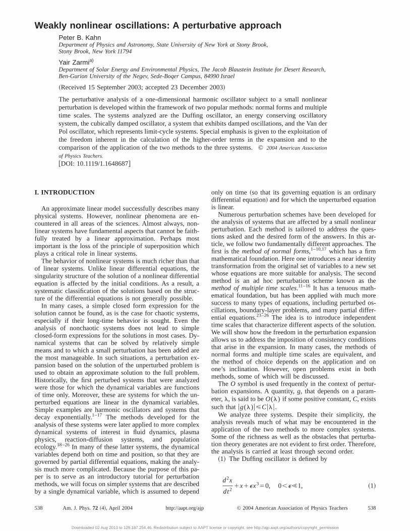
Choice of free terms. The free terms that emerge in thanalysis are an inherent feature of any perturbation theThe freedom in their choice is a reflection of the fact that odoes not aim at theexactsolution, or at a precisely specifieapproximation. Rather, one searches for an approximathat is required to be close to the correct solution withincertain error range. Technically, this results in the fact thata given order,n, of the expansion, it is impossible to distinguish between the effect of the perturbation on the timependence of the zero-order term and on the correction tof ordern. The numerical quality of the approximation is naffected by different choices of the free terms.@For example,they cannot improve the error estimate from, say,O(e) toO(e2) or vice versa.# We may choose the free terms in thexpansion@proportional toa and b in Eqs. ~34!–~37!# tosatisfy a convenient requirement. Figure 1 provides americal example of the phase-plane plot of the full solutfor the Duffing equation, together with a plot of the zerorder approximation, obtained through a first-order analywith a50. A relatively large value ofe ~e50.3! was chosento emphasize the effect of the perturbation on distortingzero-order circle.

One place where the choice of the free functions canuseful is in the calculation of the period of the oscillationwhich is given by an integral over one cycle in phase spa

T5 R dx

A2~E2V~x!!. ~38!

Here E is the total energy andV(x) is the potential. If wesubstitute the potential and the total energy for the casthe Duffing oscillator,

V~x!5 12x

21 14x

4, E5 12A

21 14A

4, ~39!

where A is the amplitude at the turning point, the integrbecomes

T54E0

A dx

A~A22x2!11

2e~A42x4!

. ~40!

This integral can be expressed in terms of a complete elliintegral of the first kind. If we evaluate the integral throuO(e4), we find an expression for the frequencyv5(2p/T) in terms of theA:

v511e3

8A22e2

21

256A41e3

81

2048A62e4

6549

262 144A8

1O~e5!. ~41!

In Eq. ~36!, v is expressed in terms ofr, the amplitude of thezero-order approximation. To properly compare Eqs.~36!and ~41!, we need to find the relation betweenr andA. Weobtain this relation by imposing the initial conditions,x(0)and dx/dt(0). Thechoice of the free functions affects threlation as well as the manner in which the phase is chan

Problem 1. Explain why the period can be calculatedfour times the integral over a quarter of the cycle and derEq. ~40!.

The choice of the free functions~the constantsa andb inthe present problem! affects the structure of the higher-ordcorrection terms in the near-identity transformation. Aspreceding analysis shows, this choice modifies the strucof the zero-order approximation. Thus, different choices



y.e

nan

-m

-

is

e

e,e:

of

l

ic

d.

e

eref

the free functions correspond to different ways of arrangthe perturbation series and shifting higher-order termstween the near-identity transformation, Eq.~8!, and the nor-mal form, Eq.~9!. Clearly, the physics of the solution cannchange, and, indeed, a detailed check17 shows that, through agiven order ine, the error incurred by using the approximasolution rather than the exact one is of the same qualitydifferent choices of the free functions. For instance, if tnear-identity transformation is carried throughO(e) and thenormal form throughO(e2), then, as Eq.~11! indicates, theerror incurred isO(e), namely, the error is bounded byCe,through times ofO(1/e) for someC.0. Although this state-ment does not depend on the choice of the free terms,constant,C, may depend on the choice.

Of special interest is theminimal normal formchoice.17,34–38 If we choosea517/64, then Eqs.~30! and~36! yield U25v250. One can show by induction thatUn

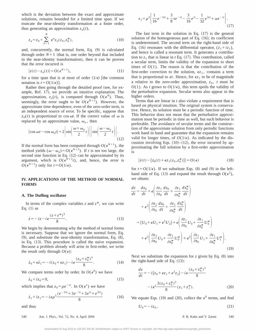
can be made to vanish for alln>2. For instance,b5131/8192 makesU3 and v3 vanish. The numerical approximations generated by the minimal normal form choice are bethan all other choices. This fact is demonstrated in Fig.where the error@the difference between the full numericsolution of Eq. ~1! and the first-order approximation# isshown for the choicea50 and the minimal normal formchoice ofa517/64.

The formal truncation of the normal form is an examplethe concept ofrenormalization. The origin of the ability toformally truncate the normal form at a finite order is thsame as for the multipole expansion of electromagnetictentials. The functional form of the first nonzero multipolephysically significant, whereas the functional form of all thhigher multipoles depends on the choice of the origin ofaxes in the frame of reference in which the expansionperformed. Similarly here, the first nontrivial correctionthe frequency~a first-order one in the case of the Duffinoscillator! is physically significant, whereas all the higheorder corrections depend on the choice of the zero-order

Fig. 1. Phase-plane plot of the solution for the Duffing oscillator we50.3,x(0)51, anddx/dt(0)50. Full solution~line! and zero-order circleapproximation~dashed line! with a50 in Eq. ~4.12!.



eea

pls

i-

ore

tedithtouth

s ins

ns,

cklyree

ng

proximation ~the analog of the choice of the origin in thmultipole expansion!. The latter is intimately related to thchoice of the free terms in each order for the following reson. A resonant term is proportional toz0

n11z0*n

5(z0z0* )nz0 . Because for a conservative system the amtude, r, is constant@see, Eq.~33!#, the free resonant termthat are included in the higher-correction termszn are pro-portional to the zero-order term,z0 . Thus, inclusion of freeresonant terms inzn amounts to shifting parts of the contrbution of the zero-order term to higher orders.

B. The oscillator with cubic damping

The main features of the solution for the Duffing oscillatare typical of conservative systems with one degree of frdom: the amplitude,r, of the zero-order term,z0 , is con-stant, and the frequency is changed by constant terms, sothe phase is justvt, with v a constant that differs from thunperturbed frequency. The structure of the solutions insipative systems is different. Both the amplitude andphase are complicated functions of time. For the oscillawith cubic damping, the solution is attracted to the origin dto damped oscillations. The calculations parallel those ofDuffing oscillator. If we use Eqs.~3!, ~6!, and ~7!, we canwrite

z52 iz2 i~z2z* !3

2i52 iz1 i

~z2z* !3

2. ~42!

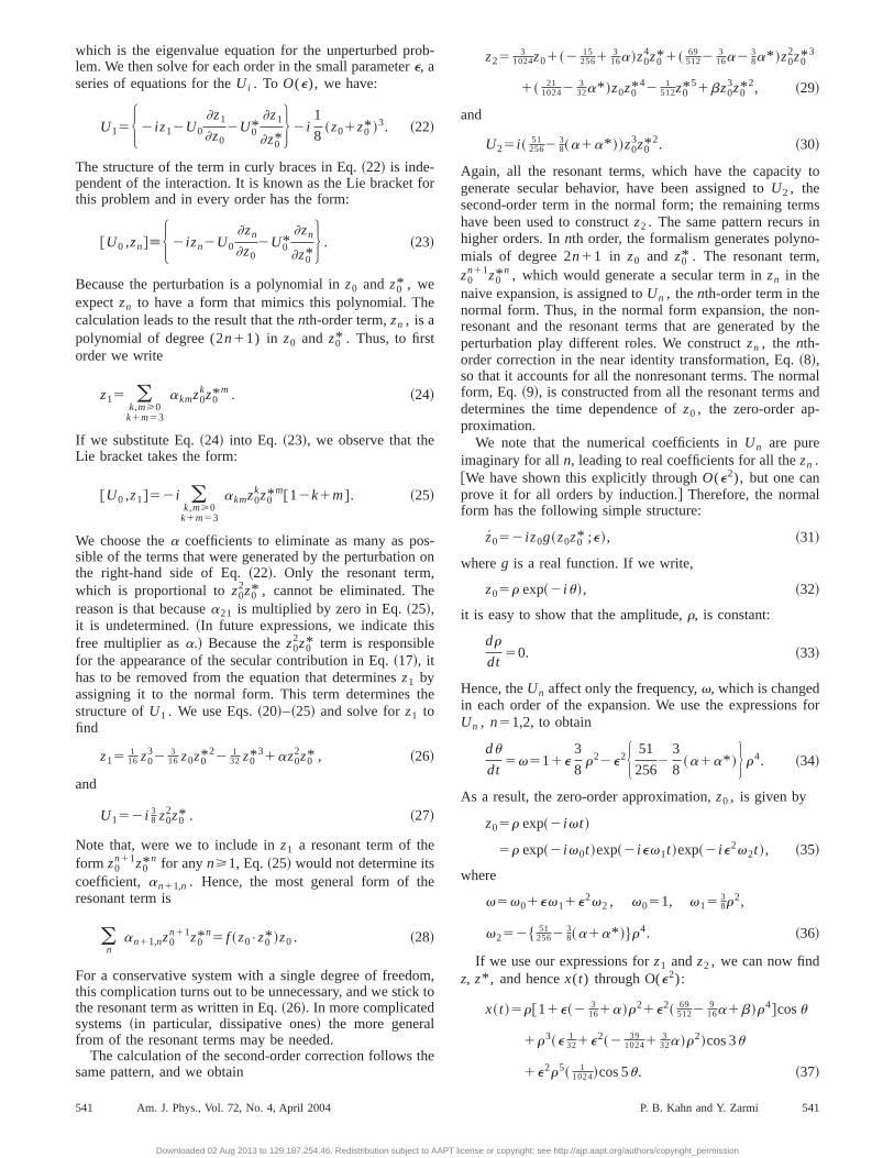
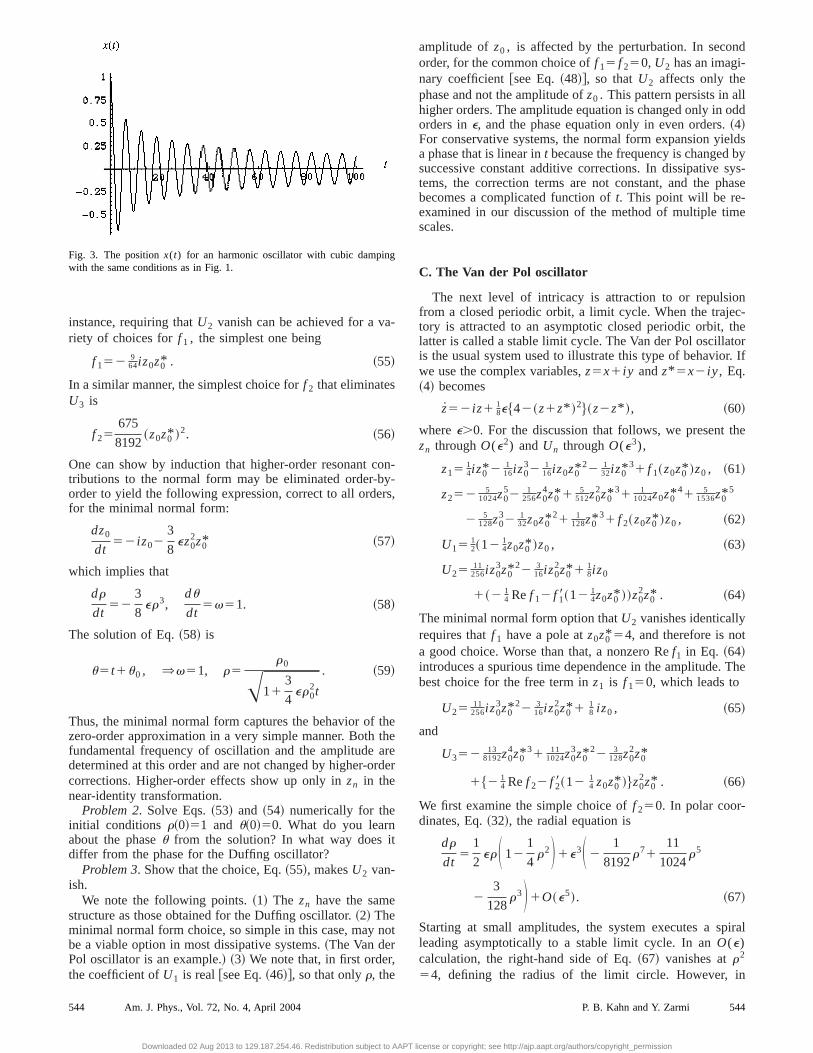
An example of the solution forx(t), which is the real part ofz(t), is given in Fig. 3.

We substitute the near-identity transformation, Eq.~8!, andthe normal form, Eq.~9!, in Eq. ~42! and obtain:

dz

dt5$U01eU11e2U2%1eS ]z1

]z0U01

]z1

]z0*U0* D

1e2S ]z2

]z0U01

]z2

]z0*U0* D 1e2S ]z1

]z0U11

]z1

]z0*U1* D

52 i $z01ez11e2z2%1e1

8~z02z0* !3

1e23

8~z02z0* !2~z11z1* !. ~43!

We collect terms as before and obtain:

U052 iz0 , ~44!

U15H 2 iz12U0

]z1

]z02U0*

]z1

]z0*J 1

~z02z0* !3

8. ~45!

If we use the expression in Eq.~24! for z1 , theO(e) part ofthe solution is

U152e 38 z0

2 z0* , ~46!

and

z15 116iz0

323

16iz0z0*

21 132iz0*

31 f 1~z0•z0* !z0 . ~47!

The last term inz1 is the free resonant term. Observe thatz1

has imaginary coefficients and thatU1 is real, indicating



-

i-

e-

hat

s-er

ee

damped motion. In a similar manner, theO(e2) terms arefound to be

U252 38~ f 11 f 1* !z0

2z0* 1 34 f 18z0

3z0*21 27

256iz03z0*

2, ~48!

z252 91024z0

51 9256z0

4z0* 2 27512z0

2z0*32 27

1024z0z0*41 3

512z0*5

1 316i f 1z0

32 316i f 1z0

2z0*22 3

8i f 1* z0z0*21 3

32i f 1* z0*2

1 f 2~z0•z0* !z0 , ~49!

where

f 185d

d~z0z0* !f 1~z0z0* !, ~50!

and a free resonant term has been included inz2 . To O(e3)we find

U352 38~2 f 1

213 f 1f 1* !z02z0* 1@ 27

128i ~ f 11 f 1* !

2 34 f 1f 18#z0

3z0*22 3

4~ f 181 f 18* ! f 18z04z0*

3

2 38~ f 21 f 2* !z0

2z0* 1 34 f 28z0

3z0*22 567

8192z04z0*

3. ~51!

We now show how the choice of the free resonant termthe generators,zn , may be exploited. If all the free termvanish (f 15 f 250 in the approximation presented here!,then the normal form is given by

dz0

dt52 iz02e

3

8z0

2z0* 1e227

256iz0

3z0*22e3

567

8192z0

4z0*3

1O~e4!. ~52!

If we use Eq.~32! for z0 , we find that Eq.~52! leads to theconclusion that is typical of dissipative systems equationamely, that both the frequency,v, and the amplitude,r,vary with time in a nontrivial manner:

dr

dt52

3

8er32

567

8192e3r71O~e4!, ~53!

du

dt5v512

27

256e2r41O~e4!. ~54!

In higher orders, the amplitude and phase equations quibecome unwieldy. However, in the present problem, the ffunctions can be chosen to eliminateUn for all n>2. For

Fig. 2. Error in the first-order approximation to the solution for the Duffioscillator with the same conditions as in Fig. 1. No free function~line! andminimal normal form~dashed line! choice.



-

oyrs

ththarrd

it

no

,

d

lodd

ldsbysys-hase

e

nc-thetorr. If

he

t

The

iral

n

g

instance, requiring thatU2 vanish can be achieved for a variety of choices forf 1 , the simplest one being

f 152 964iz0z0* . ~55!

In a similar manner, the simplest choice forf 2 that eliminatesU3 is

f 25675

8192~z0z0* !2. ~56!

One can show by induction that higher-order resonant ctributions to the normal form may be eliminated order-border to yield the following expression, correct to all ordefor the minimal normal form:

dz0

dt52 iz02

3

8ez0

2z0* ~57!

which implies that

dr

dt52

3

8er3,

du

dt5v51. ~58!

The solution of Eq.~58! is

u5t1u0 , ⇒v51, r5r0

A113

4er0

2t

. ~59!

Thus, the minimal normal form captures the behavior ofzero-order approximation in a very simple manner. Bothfundamental frequency of oscillation and the amplitudedetermined at this order and are not changed by higher-ocorrections. Higher-order effects show up only inzn in thenear-identity transformation.

Problem 2. Solve Eqs.~53! and ~54! numerically for theinitial conditions r~0!51 and u~0!50. What do you learnabout the phaseu from the solution? In what way doesdiffer from the phase for the Duffing oscillator?

Problem 3. Show that the choice, Eq.~55!, makesU2 van-ish.

We note the following points.~1! The zn have the samestructure as those obtained for the Duffing oscillator.~2! Theminimal normal form choice, so simple in this case, maybe a viable option in most dissipative systems.~The Van derPol oscillator is an example.! ~3! We note that, in first orderthe coefficient ofU1 is real@see Eq.~46!#, so that onlyr, the

Fig. 3. The positionx(t) for an harmonic oscillator with cubic dampinwith the same conditions as in Fig. 1.



n--,

eeeer

t

amplitude ofz0 , is affected by the perturbation. In seconorder, for the common choice off 15 f 250, U2 has an imagi-nary coefficient@see Eq.~48!#, so thatU2 affects only thephase and not the amplitude ofz0 . This pattern persists in alhigher orders. The amplitude equation is changed only inorders ine, and the phase equation only in even orders.~4!For conservative systems, the normal form expansion yiea phase that is linear int because the frequency is changedsuccessive constant additive corrections. In dissipativetems, the correction terms are not constant, and the pbecomes a complicated function oft. This point will be re-examined in our discussion of the method of multiple timscales.

C. The Van der Pol oscillator

The next level of intricacy is attraction to or repulsiofrom a closed periodic orbit, a limit cycle. When the trajetory is attracted to an asymptotic closed periodic orbit,latter is called a stable limit cycle. The Van der Pol oscillais the usual system used to illustrate this type of behaviowe use the complex variables,z5x1 iy andz* 5x2 iy , Eq.~4! becomes

z52 iz1 18e$42~z1z* !2%~z2z* !, ~60!

wheree.0. For the discussion that follows, we present tzn throughO(e2) andUn throughO(e3),

z15 14iz0* 2 1

16iz032 1

16iz0z0*22 1

32iz0*31 f 1~z0z0* !z0 , ~61!

z252 51024z0

52 1256z0

4z0* 1 5512z0

2z0*31 1

1024z0z0*41 5

1536z0*5

2 5128z0

32 132z0z0*

21 1128z0*

31 f 2~z0z0* !z0 , ~62!

U15 12~12 1

4z0z0* !z0 , ~63!

U25 11256iz0

3z0*22 3

16iz02z0* 1 1

8iz0

1~2 14 Ref 12 f 18~12 1

4z0z0* !!z02z0* . ~64!

The minimal normal form option thatU2 vanishes identicallyrequires thatf 1 have a pole atz0z0* 54, and therefore is noa good choice. Worse than that, a nonzero Ref1 in Eq. ~64!introduces a spurious time dependence in the amplitude.best choice for the free term inz1 is f 150, which leads to

U25 11256iz0

3z0*22 3

16iz02z0* 1 1

8 iz0 , ~65!

and

U352 138192z0

4z0*31 11

1024z03z0*

22 3128z0

2z0*

1$2 14 Ref 22 f 28~12 1

4 z0z0* !%z02z0* . ~66!

We first examine the simple choice off 250. In polar coor-dinates, Eq.~32!, the radial equation is

dr

dt5

1

2erS 12

1

4r2D1e3S 2

1

8192r71

11

1024r5

23

128r3D1O~e5!. ~67!

Starting at small amplitudes, the system executes a spleading asymptotically to a stable limit cycle. In anO(e)calculation, the right-hand side of Eq.~67! vanishes atr2

54, defining the radius of the limit circle. However, i



ur

li-

by

fre

gtiticlaac

eth

se

le, t,

.r

;

d ine

tlyckrdlymethehe,-.

na-e of

sti-the

inantfor-sthe

higher orders, the zero of the right-hand side of Eq.~67! isshifted to

r2542 316e

21O~e4!. ~68!

Thus, the radius of the limit circle is affected by the pertbation.

The equation for the~time-dependent! frequency is

v5du

dt512e2S 11

256r42

3

16r21

1

8D1O~e4!. ~69!

To obtain the asymptotic value of the frequency ast→`, wemust substitute in Eq.~69! the asymptotic value ofr, whichis given by an infinite series ine. This complication can beavoided by a radius renormalization choice forf 2 . We lookfor an f 2 that will make the asymptotic value ofr2 remain at4 when the third-order contribution is included in the amptude equation. To this end, we need to makeU3 proportionalto U1 . With U3 given by Eq.~66!, this behavior is achievedby

Ref 252 138192~z0z0* !31 11

1024~z0z0* !22 3128~z0z0* !

~ Im f 250!. ~70!

The expression forU3 becomes

U35~ 134096z0

4z0*32 11

1024z03z0*

2!~12 1

4z0z0* !. ~71!

The radial equation is modified and Eq.~67! is replaced by

dr

dt5

1

2erS 12

1

4r2D

3H 11e2S 13

2048r62

11

512r4D1O~e4!J . ~72!

Thus, the value of the limit-circle radius is unaffectedhigher-order corrections and remains fixed atr52. As a re-sult, the series for the asymptotic expression for thequency is readily obtained:

v512 116e

21O~e4!. ~73!

A detailed examination17 shows that, as expected, shiftinterms in the expansion procedure from the near-identransformation to the normal form does not alter the physThe free functions enable us to simplify parts of the calcution. However, all choices yield the same numerical accurthrough a given order.

In Fig. 4 a phase-plane plot of two solutions of Eq.~4! isshown: one spiraling toward the limit cycle from the outsidand one spiraling from the inside. To see the effect ofhigher-order terms on the solution, a limit circle ofr52 alsois plotted.

Problem 4. Solve Eq.~4! for the same initial conditions ain Fig. 4, but with e520.3. What is the behavior of thsolution?

V. THE METHOD OF MULTIPLE TIME SCALES

To motivate the introduction of the method of multiptime scales, we observe that in stable oscillatory systemstime dependence of the solution is given through a phaseu,which has the form

u5vt5S (n>0

envnD t. ~74!



-

-

ys.-y

,e

he

See, for example, Eq.~35! for the Duffing oscillator, and Eq~73! for the t→` behavior of the van der Pol limit cycle. Foueu!1 and short times@ t5O(1)#, only then50 term is im-portant, because the termsent(n>1) in Eq. ~76! are negli-gibly small and hardly affect the time dependence. Ast→O(1/e), the first two terms (n50,1) become significantwhen it becomesO(1/e2) the terms with (n50,1,2) are sig-nificant, and so on. Thus, as time increases as measurepowers of 1/e, a progressively larger number of terms in thtime dependence become significant. Thenth time scale isdefined by

Tn5ent. ~75!

When Eq.~74! applies, the phase factor, exp(2iu), can bewritten in a factorized form:

e2 iu5e2 iv0te2 iv1~et !e2 iv2~e2t !•••

5e2 iv0T0e2 iv1T1e2 iv2T2•••. ~76!

For a given duration, hardly anything happens on sufficienlong time scales~for example, as the second hand of a clomoves a few seconds, the minute and hour hands hamove!. We are, therefore, tempted to treat the various tiscales,Tn , as independent variables. This assumption isstarting point of the method of multiple time scales: Tsolution is assumed to depend on all time scalesz5z(T0 ,T1 ,T2 ,...). Hence, in addition to expanding the solution in powers ofe @the near-identity transformation, Eq~8!#, the time derivative is replaced by:

d

dt→ ]

]T01e

]

]T11e2

]

]T21•••. ~77!

The introduction of independent time scales and the elimition of secular terms lead to conditions on the dependencthe solution on the various time scales~solvability condi-tions!. For most dynamical systems, these conditions contute nontrivial consistency constraints on the structure ofapproximate solutions. In general, the freedom, enjoyedthe method of normal forms, to choose the free resonterms that appear in every order in the near-identity transmation, Eq.~8!, does not exist in the multiple time scalemethod. The consistency problems encountered inmethod are an issue of much concern.39–46

For conciseness, it is customary to use the notation

Dn[]

]Tn. ~78!

If we substitute Eqs.~8! and ~77! in Eq. ~7!, and expandthroughO(e2), we obtain

~D01eD11e2D2!~z01ez11e2z2!

52 i ~z01ez11e2z2!1 i eF~z0 ,z0* !

1 i e2H ]F~z0 ,z0* !

]z0z11

]F~z0 ,z0* !

]z0*z1* J . ~79!

We collect terms order by order and obtain

D0z01 iz050, ~80!

D0z11 iz152D1z01F~z0 ,z0* !, ~81!



w-nl

d

rt

w-

n

t i

la

tll

s

n-

r,arte

-

of

r of

ns,n-

oftheith

st-

q.

ith

D0z21 iz252D1z12D2z01]F~z0 ,z0* !

]z0z1

1]F~z0 ,z0* !

]z0*z1* . ~82!

Equation~80! is readily solved by

z05A~T1 ,T2!e2 iT0. ~83!

The amplitude,A, depends on all higher time scales. Hoever, because we will limit our analysis to second order, oT1 andT2 have been written out explicitly.

Although the analysis of Eq.~81! depends on the detailestructure of the perturbation,F(z0 ,z0* ), the following canalready be said at this point. First, the homogeneous pathe equation,

D0z11 iz150, ~84!

introduces a contributionz1 which we write in the form

B~T1!e2 iT0. ~85!

The amplitudeB may depend on all higher time scales. Hoever, in a second-order analysis, only itsT1 dependencecounts. Second, any term on the right-hand side of Eq.~81!whoseT0 dependence is of the form exp(2iT0) resonateswith the left-hand side of the equation, and hence will geerate inz1 a term that is linear inT0 ~a secular term!. Suchterms must be eliminated to yield an approximation thavalid for times ofO(1/e) and not just ofO(1). There is anexplicit term of this kind, namely,2D1z0 . In addition, anymonomial of the formz0

n11 z0*n in F(z0 ,z0* ) will have this

T0 dependence. We denote the resonant part ofF(z0 ,z0* ) byF(z0 ,z0* )R . To eliminate all the terms that generate secubehavior, we impose the requirement

2D1z01F~z0 ,z0* !R50. ~86!

This first-order solvability condition determines theT1 de-pendence of the amplitudeA of Eq. ~83!. Once the resonanterm in Eq. ~81! has been removed, we can find the fu

Fig. 4. Phase-plane plot of a solution of the Van der Pol oscillator we50.3. Solution of Eq.~4.35! ~full line!, limit cycle ~thick lime!, limit circlewith radius52 ~dashed line!.



y

of

-

s

r

solution for z1 , including the solution of the homogeneouequation:

z15 z11B~T1!e2 iT0, ~87!

wherez1 is the particular solution that accounts for the noresonant contribution ofF(z0 ,z0* ) in Eq. ~81!.

With z1 known, Eq.~82! is analyzed in a similar manneandz2 also will include a solution of the homogeneous pof Eq. ~82!. To avoid secular terms, the contribution of all thresonant terms on the right-hand side of Eq.~82! has to van-ish, leading to the second-order solvability condition:

S 2D1z12D2z01]F~z0 ,z0* !

]z0z11

]F~z0 ,z0* !

]z0*z1* D

R

50.

~88!

Equation~88! determines theT1 dependence of the amplitudeB. Consistency between Eqs.~86! and~88! will turn outto be a major limitation on the application of the methodmultiple time scales.

As in the method of normal forms@see Eqs.~11! and~12!#,a comment is in order regarding error estimates. An errothe magnitude defined by Eq.~11! is obtained if the near-identity transformation contains higher-order correctiothroughO(eN), as in Eq.~10!. Concurrently, for each termzk , k<N, in the approximate solution, we find the depedence ofzk on T0 , T1 ,...,TN112k . Thus, we have to find thedependence ofz0 on T0 , T1 ,...,TN11 , of z1 on T0 ,T1 ,...,TN , of z2 on T0 , T1 ,...,TN21 , etc. A major point thatwe will discuss in the following is that often the methodmultiple time scales does not yield the dependence onhigher time scales, and we must augment the method wadditional information to find that dependence.

VI. APPLICATIONS OF THE METHOD OFMULTIPLE TIME SCALES

A. The Duffing oscillator

For F(z0 ,z0* ) of the Duffing oscillator@see Eq.~6!#, and~83! for z0 , Eq. ~81! becomes

D0z11 iz152D1Ae2 iT02 18iA

3e23iT02 38iA

2A* e2 iT0

2 38iAA* 2eiT02 1

8iA* 3e3iT0. ~89!

The first and third terms on the right-hand side of Eq.~89!are the resonant terms. Their elimination yields the firorder solvability condition,

D1A52 38iA

2A* . ~90!

If we write A in the form,

A5uAue2 iwA, ~91!

we readily find

D1uAu50, wA5 38uAu2T11cA~T2!. ~92!

Thus, the magnitude of the amplitudeA is independent ofT1 , and hence its phase is linear inT1 .

Now that we have eliminated the resonant terms in E~89!, the solution forz1 is readily found to be

z15 116A

3e23iT02 316AA* 2eiT02 1

32A* 3e3iT01Be2 iT0.~93!



.

-

a

a

eteth

yro-

t,

dic

ch

thec-en-

ers

We turn to theO(e2) equation, Eq.~82!, and substitute Eqs~90! and~93!, together withF(z0 ,z0* ) of Eq. ~6!, in Eq. ~82!,to obtain

D0z21 iz252D1$1

16A3e23iT02 3

16AA* 2eiT0

2 132A* 3e3iT01Be2 iT0%2D2Ae2 iT0

1 38~Ae2 iT01A* eiT0!2$ 1

32A3e23iT0

2 316A

2A* e2 iT02 316AA* 2eiT01 1

32A* 3e3iT0

1Be2 iT0%. ~94!

To avoid secular terms inz2 , all the terms that are proportional to exp(2iT0) must be eliminated from Eq.~94!. Thiscondition yields the second-order solvability condition:

D2A1D1B5 51256iA

3A* 22 34iAA* B2 3

8iA2B* . ~95!

Equation~95! and its complex conjugate may be regardedlinear, first-order differential equations for theT1 depen-dence ofB andB* . However, because it contains the derivtive of the amplitudeA with respect toT2 , it also can beviewed as a constraint onA. Thus, we must check if the twosolvability constraints, Eqs.~90! and~95!, are mutually con-sistent. This check can be done by either solving Eqs.~90!and ~95! directly or by requiring that derivatives ofA withrespect toT2 andT1 commute,

D1D2A5D2D1A, ~96!

when the derivativeD2 is applied to Eq.~90! and D1 isapplied to Eq.~95!. For the Duffing oscillator, both ways arsimple and easy to implement, while in more complicasystems, one way may be more advantageous than the oWe now perform the analysis in these two ways.

Problem 5. Derive Eq.~95!.Direct solution of solvability conditions. If we multiply

Eq. ~97! by A* and its complex conjugate byA and use Eq.~90!, we obtain

D1~A* B1AB* !1D2~AA* !50, ~97!

D1~A* B2AB* !22iAA* D2wA

52 34iAA* ~A* B1AB* !1 51

128i ~AA* !3. ~98!

BecauseuAu is independent ofT1 @see Eq.~92!#, the termD2(AA* ) in Eq. ~97! also is independent ofT1 . Hence, thesolution forA* B1AB* is

~A* B1AB* !52D2~AA* !T11H~T2 ,T3 ,...!. ~99!

Consequently, Eq.~98! generates in (A* B2AB* ) terms thatare linear and quadratic inT1 :

~A* B2AB* !5 i $~2AA* D2wA1 51128~AA* !3

2 34 AA* H~T2 ,T3 ,...!!T1

1 38AA* D2~AA* !T1

21J~T2 ,T3 ,...!%.

~100!

Equations~99! and~100! yield the general solution ofB withH andJ real-valued functions.



s

-

der.

Over the time spant5O(1/e) for which the approxima-tion is valid, powers ofT1 in B need not be eliminated: Thedo not spoil the ordering of the expansion in terms of pgressively smaller terms, becauseeB contains contributionsproportional to

eT1q5e~et !q '

t5O~1/e!

O~e!. ~101!

Problem 6. What happens to the magnitude of (A* B1AB* ) of Eq. ~99! for t5O(1/e2)?

TheT2 dependence ofA is undetermined by Eqs.~90! and~95!. To specify it, we must either provide additional inpuextraneous to the method, for example, initial data forT1

50. A common way to fix theT2 dependence ofA is torequire that the solution be constructed solely out of periofunctions. To avoid aperiodic terms, Eq.~97! must be brokeninto

D2~AA* !50, D1~A* B1AB* !50, ~102!

which implies that

~A* B1AB* !5H~T2 ,T3 ,...!. ~103!

Hence,uAu is independent also ofT2 . If we use the samereasoning in Eq.~98!, we must require

wA53

8~AA* !T12

51

256~AA* !2T2

1E0

T2 3

8~A* B1AB* !dT21xA~T3 ,T4 ,...!, ~104!

and

D1~A* B2AB* !50, ~105!

which implies

~A* B2AB* !5 iJ~T2 ,T3 ,...!. ~106!

Consequently, we find that, throughO(e2), the dependenceof A on T1 andT2 factors into a product of phase terms, eadepending on one time scale only@although theT2 depen-dence of (A* B1AB* ) is still unknown#:

A5uAue2 iT0 expS 2 i3

8~AA* !T1DexpS i H 51

256~AA* !2T2

2E0

T2 3

8~A* B1AB* !dT2J D e2 ixA~T3 ,T4 ,...!. ~107!

This pattern recurs in higher orders if we require thatsolvability conditions be satisfied solely by periodic funtions. If this requirement is not imposed, then the depdence of the amplitudes on higher time scales,Tn , n>2,depends on our choice of the initial data at, say,T150.

With the choice that the solution does not contain powof T1 , Eqs.~103!, ~106!, and~90! lead to



nc

arrswtoeo

n

er

f

thon

e

b

f

glth,n

s-ed.areon-

reeoiceieldhetheof

or-lethats ofion,ee-

r thesisre-

Eqs.

fuse

D1~A* B!50

⇒D1B

523

8iAA* B

⇒H B~T1 ,T2 ,...!5uBue2 i ~3/8!~AA* !T1eicB~T2 ,T3 ,...!

D1~BB* !50~108!

Note that theT2 dependence ofA still cannot be determinedunless additional input is provided. Part of the dependehas been found due to the requirement that, throughO(e2),the solution does not contain powers ofT1 . This requirementled to the result thatuAu does not depend onT2 . However, itis not obvious that the choices made up to this pointconsistent with the solvability conditions in higher ordeBecause we have limited our analysis to second order,only state the answer: For the case of the Duffing oscilla~and all single-oscillator systems with energy conserving pturbations!, the choices are consistent. Finally, we still do nknow the dependence ofwA , the phase ofA, on T2 . Helpcomes from observing that, in this order, the solvability coditions leaveuBu free, allowing, in particular,uBu50. Thischoice completes theT2 dependence ofA and yields a simpleexpression forwA :

wA52 38~AA* !T11 51

256~AA* !2T21xA~T3 ,T4 ,...!.~109!

Note that theT1 dependence ofwB , the phase ofB, is thesame as that ofwA , leading to another choice forB that hasaesthetic appeal~and also is consistent with the higher-ordsolvability conditions!:

B5 1764A

2A* . ~110!

With this choice.wA , and, hence,A, become independent oT2 , and Eq.~104! becomes

wA5 38~AA* !T11xA~T3 ,T4 ,...!. ~111!

In the analysis in higher orders, the requirement thatdependence of the amplitudes be expressed in terms ofperiodic functions~that is, exponential phase factors!, im-plies thatA, B, and the free amplitudes that appear in highorders will all have the same time dependent phases.

Consistency of solvability conditions. The constraint forconsistency between the two solvability conditions is otained by applyingD2 to Eq. ~90!, D1 to Eq. ~95!, and re-quiring that Eq.~96! be obeyed@using Eq.~95! repeatedly#.The result yields theT1 dependence ofB:

D12B1 3

2i ~AA* !D1B1 34iA

2D1B* 2 2764~AA* !2B

1 932~AA* !A2B* 50. ~112!

Because Eq.~112! is homogeneous,B50 is an allowedchoice. Similarly, the use of Eq.~90! shows that the choice oEq. ~110! also is an allowed solution of Eq.~112!.

We end our analysis of the Duffing oscillator by notinthat the multiple time scales results are completely parallethose of the method of normal forms. For instance, inlatter method, the free term inz1 is a resonant term, that isproportional toz0 @see Eq.~26!#. The equivalent statement ithe multiple time scales method, if the time dependencethe solution is constructed only from periodic functions~that



e

e.err-t

-

ely

r

-

toe

of

is, there are no powers ofT1 in the solution!, is thatB has thesame phase asA. Also, the choiceB50 is the equivalent tothe choicea50 in Eq.~26!, and the choice of Eq.~110! is theequivalent of the minimal normal form choice ofa517/64,mentioned toward the end of Sec. IV A.

B. The oscillator with cubic damping

The Duffing oscillator is representative of dynamical sytems to which an energy conserving perturbation is addThe methods of normal forms and multiple time scalescompletely equivalent, and there is a one-to-one correspdence of the results. In particular, any choice of the fterms in the normal form analysis has a corresponding chin the multiple time scales analysis and both methods ythe same functional form for the approximate solution. Ttwo examples of dissipative systems to be discussed infollowing represent obstacles encountered in the methodmultiple time scales, which are not encountered in the nmal form analysis. These difficulties occur in the multiptime scales analysis of most linear dynamical systemsare subject to a nonlinear perturbation, be they systemone degree of freedom with a nonconservative perturbator Hamiltonian systems with more than one degree of frdom.

Because the analysis has been presented in detail foDuffing oscillator, we skip some of the steps in the analyof the cubically damped oscillator, and only discuss thesults and the important points. The zero-order solution,z0 , isgiven by Eq.~83!. The first-order correction is found to be

z15 116iA

3e23iT02 316iAA* 2eiT01 1

32iA* 3e3iT01Be2 iT0.~113!

The first- and second-order solvability conditions are

D1A52~ 38!A

2A* , ~114!

D2A1D1B5 27256iA

3A* 22 34 AA* B2 3

8 A2B* . ~115!

Direct solution of solvability conditions. If we write A asin Eq. ~91!, Eq. ~114! is solved by

D1~AA* !52 34~AA* !2, D1wA50, ~116!

leading to

A5A~AA* !0Y S 113

4~AA* !0T1De2 iwA~T2 ,T3!,

~117!

where (AA* )0 does not depend onT1 . If we multiply Eq.~115! by A* , and its complex conjugate equation byA, andsum or subtract the results, we find after repeated use of~114! and ~115!:

D1$~A* B1AB* !/~AA* !2%2D2~1/~AA* !!50, ~118!

D1$~A* B2AB* !/~AA* !1 932i ~AA* !%12iD 2wA50.

~119!

We use Eq.~117! and solve Eq.~118! to find

~A* B1AB* !5$D2~1/~AA* !0!T11H~T2 , . . . !%

3~AA* !2. ~120!

TheT1 linear term in Eq.~120! does not spoil the ordering othe magnitude of the zero- and first-order terms, beca



s-hes

to

the

urb

r-

he.einnc

ed

t

ee-

es

Eq.

ks.ofys,nsthees

e

y

thanks to Eq.~117!, this term generatesO(T121) leading be-

havior in (A* B1AB* ).Equation~119! is solved by

~A* B2AB* !5$2 932i ~AA* !22iD 2wAT1

1 iJ~T2 , . . . !%~AA* !. ~121!

By using Eqs.~12! and ~121!, the solution forB is found tobe

B5$@ 12H~T2 , . . . !2 9

64i #AA* 1 12@D2~1/~AA* !0AA* T1

1 iJ~T2 , . . . !!#%A2 iD 2wAAT1 . ~122!

Here,H andJ are real valued functions of higher time scaleAgain, theT2 dependence ofA is not specified; its determination requires additional input that is not provided by tmethod of multiple time scales and may be fixed as followThe last term in Eq.~122! generates a term proportionalT1

1/2 in B. For the allowed time span,t5O(1/e), for whichthe approximation is valid, this term does not destroyordering in the near-identity transformation. However, bcause aT1

1/2 term does not agree with the expected structof the approximate solution, it makes sense to eliminate itrequiring that

D2wA50. ~123!

With this choice, there is no secular behavior inB, becauseits asymptoticT1 dependence becomes that ofA, namely,O(T1

21/2). Hence, there is no constraint onD2(1/(AA* )0) inEq. ~122!, and, without additional input, we cannot detemine the T2 dependence ofA. An appealing choice is toassume thatA does not depend onT2 . To this end, we haveto add to Eq.~123! the requirement that

D2~1/~AA* !0!50. ~124!

Equation~122! for B then becomes

B5$ 12H~T2 , . . . !2 9

64i %A2A* 1 1

2iJ~T2 , . . . !A. ~125!

Note that the first-order minimal normal form choice of tnormal form analysis, Eq.~55!, is a particular case of Eq~125!, with J5H50. This latter choice is consistent with thtwo solvability conditions. It turns out that the analysishigher orders allows for the cancellation of the dependeof A on the higher time scales (T3 ,...) aswell. This cancel-lation is a reflection of the fact that for the cubically damposcillator, only two time scales,T0 and T1 , are required todescribe the physics. However, the equivalence betweenmethods of normal forms and multiple time scales endsthis point. For example, in the normal form analysis wcould chose the free resonant term to vanish, but herB50 is allowed only in the trivial case,A50, as can be deduced directly by a detailed inspection of Eqs.~114! and~115!, or the solution forB given by Eq.~122!.

Problem 7. What happens to the magnitude ofB of Eq.~122! for t5O(1/e2)? Use Eq.~117!.

Consistency of solvability conditions. The same conclu-sions regarding the constraints onB may be reached moreasily by the requirement that the two solvability conditionEqs.~114! and~115!, are mutually consistent. If we applyD2

to Eq. ~114! and D1 to Eq. ~115! and impose Eq.~96!, weobtain:



.

.

e-ey

e

heat

,

D12B1 3

2~AA* !D1B1 34A

2D1B* 1 964~AA* !2B

1 932~AA* !A2B* 1 81

512iA4A* 350. ~126!

Clearly, B50 is allowed only for the trivial caseA50. Onthe other hand, a detailed check shows that the choice of~125! is an allowed solution of Eq.~126!, and hence is con-sistent with both solvability conditions, Eqs.~114! and~115!.

In summary, we have to overcome two stumbling blocFirst, unlike the Duffing oscillator, the freedom of choicethe free amplitudes, which the normal form analysis enjois lost due to the requirement that the solvability conditiofor different orders be mutually consistent. Second, as forDuffing oscillator, the method of multiple time scales donot provide the dependence of the solution onT2 , or, for thatmatter, any time scales beyondT1 , without additional infor-mation, consistent with the solvability conditions.

Problem 8. Prove the statement following Eq.~126!.

C. The Van der Pol oscillator

We follow the steps given in detail in Sec. IV, employ thsame notation, and obtain the first-order results:

D1A5 12A~12 1

4AA* !, ~127!

z152 116iA

3e23iT01$2 116AA* 21 1

4A* % ieiT0

2 132iA* 3e3iT01Be2 iT0. ~128!

The second-order analysis yields

D1B1D2A5 12B2 1

4AA* B2 18A

2B* 1 18iA2 3

16iA2A*

1 11256iA

3A* 2, ~129!

z252 51024A

5e25iT01$ 1256A

4A* 2 5128A

32 316iA

2B%e23iT0

1$ 5512A

2A* 32 132AA* 21 1

4iB* 2 116iA* 2B

2 18iAA* B* %eiT01$ 1

128A* 31 11024AA* 4

2 332iA* 2B* %e3iT01 5

1536A* 5e5iT01Ce2 iT0. ~130!

Direct solution of solvability conditions. Equation~127!yields

D1~AA* !5AA* S 121

4AA* D , ~131!

D1wA50. ~132!

Equation~131! is solved by

AA* 54~AA* !0

~~AA* !01~42~AA* !0!exp~2T1!!. ~133!

wA and (AA* )0 do not depend onT1 , but may be functionsof T2 , T3 ,... .

We multiply Eq. ~129! by A* and employ Eqs.~127!,~129!, ~132!, and~133!, and obtain for the real and imaginarparts:

D1H exp~T1!~A* B1AB* !

~AA* !2 J5D2S exp~T1!

~AA* ! D5D2S 1

~AA* !0D , ~134!



s-

id

eoiuul.or

orce

lly

ho-

esd

er

Inas

the

od

ethee

D2wA21

165D1H 2

~A* B2AB* !

2iAA*

11

16log~AA* !2

11

64~AA* !J . ~135!

Equation~134! is solved by

~A* B1AB* !5exp~2T1!S G~T2 ,T3 , . . . !

1D2S 1

~AA* !0DT1D ~AA* !2, ~136!

whereG is a free real-valued function. Although all the termin Eq. ~136! fall off exponentially, their ordering in the perturbation series is destroyed if theT1 linear term is not elimi-nated in Eq.~136!. To eliminate this term, we impose

D2~AA* !050⇒D2~AA* !50, ~137!

~A* B1AB* !5exp~2T1!G~T2 ,T3 , . . . !~AA* !2.~138!

We note that the left-hand side of Eq.~135! is independent ofT1 @see Eq.~132!#. The integration of Eq.~135! over T1 ,therefore, yields~with H a real valued function!:

S D2wA21

16DT152~A* B2AB!

2iAA*1 1

16 log~AA* !

2 1164~AA* !1H~T2 ,T3 , . . . !. ~139!

The last three terms on the right-hand side of Eq.~139! can-not counterbalance the linear behavior of the left-hand sfor T1→`. Hence, to avoid aT1 secular term inB, theleft-hand side of Eq.~139! must vanish, yielding

D2wA5 116⇒wA5 1

16T21cA~T3 ,T4 , . . . !, ~140!

~A* B2AB* !5$ 116 log~AA* !2 11

64~AA* !

1H~T2 ,T3 , . . . !%2i ~AA* !. ~141!

From Eqs.~138! and ~141!, we find

B5$ 12G~T2 ,T3 , . . . !exp~2T1!~AA* !

1 iH ~T2 ,T3 , . . . !1 116i log~AA* !2 11

64i ~AA* !%A.

~142!

The characteristics of the solution are obviously the samin the method of normal forms. Namely, through secondder, the zero-order term asymptotes to a limit circle of rad2. Had we continued the analysis to third order, we wohave found ane2 correction to the radius of the limit circleHowever, here comes the difference. In the method of nmal forms, we saw that it is possible to choose the free tein first order to vanish@ f 1 of Eq. ~61!#. The equivalent re-quirement here is

B[0. ~143!

However, unlike the energy conserving Duffing oscillatthe solvability conditions impose restrictions on this choiFrom Eq.~142! we find that due to theT1 dependence ofA,Eq. ~143! is satisfied only if the solution vanishes identicaor is already on the limit cycle:

A50, ~144!



e

asr-sd

r-m

,.

AA* [4. ~145!

The choice of Eq.~145! makes AA* independent of allhigher time scales. That is, the zero-order term must be csen as the asymptotic circle with radius 2:

A52ei ~~1/16!T21cA~T3 ,T4 , . . . !!. ~146!

Equations~145! and ~146! imply that z0 and z1 are bothconfined to their asymptotic limit. Hence, this choice donot cover situations in which the initial condition is removefrom the limit cycle byO(e) or O(1), so that exponentialspiraling toward the limit cycle occurs only in orders highthan first.

TheT2 dependence of the phase,wA , given by Eq.~140!,is required for consistency with the solvability conditions.the normal forms method, this behavior is attained onlyT2→`. For example, if we use Eqs.~63! and ~64! for U1

andU2 , respectively, the normal form, Eq.~9! becomes

z052 iz01 12 e~12 1

4z0z0* !z01e2$2@ 14 Ref 1~z0z0* !

1 f 18~z0z0* !~12 14 z0z0* !#z0

2z0* 1 11256iz0

3z0*22 3

16iz02z0*

1 18iz0%. ~147!

The first-order term in Eq.~147! ensures thatr→2 as t→`. Through second order, the time dependence ofphase is

dwA

dt52e2H 11

256r42

3

16r21

1

82Im f 18~r2!S 12

1

4r2D r2J .

~148!Thus, in general, Eq.~140! of the method of multiple timescales is reached only fort→`. To obtain Eq.~140! as theexacte2 dependence ofwA in the normal forms analysis, wemust choose for the free function,f 1 :

Im f 1~r2!5 116 ln r22 11

64r21C, ~149!

whereC is an arbitrary constant. In the normal forms meththis is a possible choice. Equation~142! shows that in mul-tiple time scales it is the only possibility.

Consistency of solvability conditions. If we apply the de-rivative D1 to Eq. ~129! and D2 to Eq. ~127! and use bothequations repeatedly, we find that Eq.~96! leads to:

D12B2D1B1 1

2AA* D1B1 14A

2D1B* 1 14B1 1

64~AA* !2B

1 132A

3A* B* 1 316iA

2A* 2 17128iA

3A* 21 11512iA

4A* 350.~150!

If we multiply Eq. ~150! by A* , we obtain for the real andimaginary parts:

D12$exp~T1!~A* B1AB* !/~AA* !2%50, ~151!

D12H ~A* B2AB* !

~AA* !1

1

8i log~AA* !2

11

32i AA* J 50.

~152!

A detailed analysis shows that Eqs.~151! and~152! are con-sistent with Eqs.~134! and ~139!, respectively, from whichthe solution forB, Eq. ~142!, has been obtained. Hence, thconsistency test is equivalent to the direct analysis ofsolution of the solvability conditions. In particular, thchoiceB50, is consistent with Eq.~152! only for A50 orAA* 54.



oansibj

oodit

tubothio

tanroTail aa

dorrth

haosipbo

idthemmtivthyethneg

-le

ethlyulbsiettsvedeub

oeur

a

reing

pleap-

pen

-

al

est.

s,’’

al

s

nd

r

-

-

ve

’’

of

s,ge,

lib-

r,’’

VII. CONCLUDING COMMENTS

Our goal has been to give a tutorial on the applicationtwo commonly used perturbation methods, normal formsmultiple time scales. To simplify the discussion, the analyhas been confined to single oscillator systems that are suto nonlinear perturbations. We have shown the effectstypical nonlinear perturbations: modification of the perifor energy conserving perturbations and damping- or limcycle phenomena for dissipative perturbations. Both perbation methods focus on the manner in which the perturtion modifies the zero-order approximation in compariswith the naive expansion. In both methods, the effect ofperturbation on the solution for the zero-order approximatis identified as the resonant terms that are generated byperturbation in every order. If, as is done in the naive expsion, they are not accounted for by their effect on the zeorder term, they lead to the emergence of secular terms.goal is to generate a zero-order approximation that contthe major physical effects of the perturbation, but is stilsmall modification of the solution of the unperturbed eqution.

Our analysis has stressed the role played by the freeinherent in perturbation theory. There is a one-to-one cospondence between the exploitation of this freedom inapplication of the two methods to a harmonic oscillator tis modified by an energy conserving perturbation. This crespondence is lost when the methods are applied to distive systems for which only a subset of the choices availain the method of normal forms is allowed in the methodmultiple time scales.

Because both methods have been applied to a much wclass of systems, we know that the loss of freedom inmultiple time scales method extends beyond the systwith a single degree of freedom and applies to most dynacal systems of physical interest. We provide here an intuiargument. Consider a system of two harmonic oscillatorshave equal unperturbed frequencies and are coupled benergy conserving interaction. The combined system isergy conserving. However, because of the equality ofunperturbed frequencies, energy flows efficiently back aforth between the two oscillators due to the coupling btween them. ‘‘Efficiently’’ means that, although the couplinis weak, characterized by a small parameter,e, the energyflow between the two oscillators, while slow@becoming sig-nificant only for t5O(1/e)], is not small. Thus, each subsystem looks like a dissipative one. The multiple time scaanalysis of this system reveals that the freedom of choicthe free amplitudes is limited by the requirement thatsolvability conditions for different orders be mutualconsistent.46 The same applies to the application of the mtiple time scales method to systems described by PDEs,cause they are systems with an infinite number of degreefreedom.~For example, expanding the solution in a Fourseries in the spatial coordinate, leads to an infinite seODEs for the time dependence of the Fourier coefficien!The lesson from the examples discussed here is that in eapplication of the method that goes beyond a first-oranalysis, the choices made for the perturbative solution mensure that the solvability conditions for different ordersobeyed in a mutually consistent manner.

The application of the normal forms method to systemsphysical interest of spatial extent encounters other unpected difficulties. For example, if a small nonlinear pert



fdsectf

-r-a-nenhe--

hens

-

me-et

r-a-

lef

eres

i-eatann-ed-

sofe

-e-ofrof.ryrste

fx--

bation is added to the Burgers equation~which describes thepropagation of shock waves in a fluid or traffic flow onhighway! or the Korteweg–de Vries equation~which de-scribes the propagation of shallow water waves!, then newconsistency problems called ‘‘obstacles to integrability’’ aencountered.18–22The unperturbed equations have interestnonlinear wave solutions~for example, solitons!. Often, theperturbative expansion generates terms that spoil the simstructure of the unperturbed solution, and the zero-orderproximation~which is determined by the normal form! maynot have the same wave structure. The resolution of this oproblem is under investigation.47

a!Electronic mail: [email protected]. Poincare´, New Methods of Celestial Mechanics, originally published asLes Methodes Nouvelles de la Mechanique Celeste~Gauthier-Villars,Paris, 1892! and ~AIP Press, New York, 1993!.

2G. D. Birkhoff, Dynamical Systems~American Mathematical Society Colloquium, New York, 1927!.

3G. I. Hori, ‘‘Theory of general perturbations with unspecified canonicvariables,’’ Publ. Astron. Soc. Jpn.18, 287–296~1966!.

4A. Deprit, ‘‘Canonical transformations depending on a parameter,’’ CelMech.1, 12–13~1969!.

5G. I. Hori, ‘‘Theory of general perturbations for non-canonical systemPubl. Astron. Soc. Jpn.23, 567–587~1971!.

6V. I. Arnold, Geometrical Methods in the Theory of Ordinary DifferentiEquations~Springer-Verlag, New York, 1988!, 2nd ed.

7A. D. Bruno, Local Methods in Nonlinear Differential Equation~Springer-Verlag, New York, 1989!.

8A. H. Nayfeh,Method of Normal Forms~Wiley, New York, 1993!.9J. Guckenheimer and P. J. Holmes,Nonlinear Oscillations, DynamicalSystems, and Bifurcations of Vector Fields~Springer-Verlag, New York,1988!.

10S. Wiggins, Introduction to Applied Nonlinear Dynamical Systems aChaos~Springer-Verlag, New York, 1990!.

11A. H. Nayfeh,Perturbation Methods~Wiley, New York, 1973!.12C. M. Bender and S. A. Orszag,Advanced Mathematical Methods fo

Scientists and Engineers~McGraw–Hill, New York, 1978!.13A. H. Nayfeh,Introduction to Perturbation Techniques~Wiley, New York,

1981!.14J. Kevorkian and J. D. Cole,Perturbation Methods in Applied Mathemat

ics ~Springer-Verlag, New York, 1985!.15J. A. Murdock, Perturbation Theory and Methods~Wiley, New York,

1991!.16J. Kevorkian and J. D. Cole,Multiple Scale and Singular Perturbation

Methods~Springer-Verlag, New York, 1996!.17P. B. Kahn and Y. Zarmi,Nonlinear-Dynamics: Exploration Through Nor

mal Forms~Wiley, New York, 1998!.18Y. Kodama and T. Taniuti, ‘‘Higher order approximation in the reducti

perturbative method,’’ J. Phys. Soc. Jpn.45, 298–310~1978!.19A. S. Fokas and Q. M. Liu, ‘‘Asymptotic integrability of water waves,

Phys. Rev. Lett.77, 2347–2351~1996!.20Y. Kodama, ‘‘Normal form and solitons,’’ inTopics in Soliton Theory and

Exactly Solvable Nonlinear Equation, edited by M. J. Ablowitzet al.~World Scientific, Singapore, 1987!, pp. 319–340.

21R. A. Kraenkel, J. G. Pereira, and E. C. de Rey Neto, ‘‘Linearizabilitythe perturbed Burgers equation,’’ Phys. Rev. E58, 2526–2530~1998!.

22Y. Hiraoka and Y. Kodama, ‘‘Normal form and solitons,’’ Lecture noteEuro Summer School 2001, The Isaac Newton Institute, Cambrid15–25 August, 2002 and arXiv:nlin.SI/0206021.

23A. C. Newell, ‘‘Envelope equations,’’ Lect. Appl. Math.15, 157–163~1974!.

24Y. Kuramoto, Chemical Oscillations, Waves and Turbulence~Springer-Verlag, New York, 1984!.

25P. Manneville,Dissipative Structures and Weak Turbulence~Academic,New York, 1990!.

26C. M. Cross and P. C. Hohenberg, ‘‘Pattern formation outside of equirium,’’ Rev. Mod. Phys.65, 851–112~1993!.

27B. Van der Pol, ‘‘On oscillation hysteresis in a simple triode generatoPhilos. Mag.43, 700–719~1926!.



e

it

onoc

J.

s

c.

x-

D

to

s in

pl.

e-

r

ur-

o-nt. J.

v. A

28Lord Rayleigh~J. W. Strutt!, ‘‘On maintained vibrations,’’ Philos. Mag.XV , 229–232~1883!.

29M. Kummer, ‘‘How to avoid secular terms in classical and quantum mchanics,’’ Nuovo Cimento Soc. Ital. Fis., B1B, 123–129~1971!.

30J. C. Liu, ‘‘The uniqueness of normal forms via Lie transformations andapplication to Hamiltonian systems,’’ Celest. Mech.36, 89–95~1985!.

31J. C. Van der Meer,The Hamiltonian Hopf Bifurcation~Springer-Verlag,New York, 1985!.

32A. Baider and R. C. Churchill, ‘‘Uniqueness and non-uniqueness of nuniqueness of normal form expansions for vector fields,’’ Proc. R. SEdinburgh, Sect. A: Math.108, 27–33~1988!.

33A. Baider, ‘‘Unique normal forms for vector fields and Hamiltonians,’’Diff. Eqns. 78, 33–39~1989!.

34P. B. Kahn and Y. Zarmi, ‘‘Minimal normal forms in harmonic oscillationwith small nonlinear perturbations,’’ Physica D54, 65–74~1991!.

35P. B. Kahn and Y. Zarmi, ‘‘Radius renormalization in limit cycles,’’ ProR. Soc. London, Ser. A440, 189–199~1993!.

36P. B. Kahn, D. Murray, and Y. Zarmi, ‘‘Freedom in small parameter epansion for nonlinear perturbations,’’ Proc. R. Soc. London, Ser. A443,83–94~1993!.

37E. Forest and D. Murray, ‘‘Freedom in minimal normal forms,’’ Physica74, 181–196~1994!.

38P. B. Kahn and Y. Zarmi, ‘‘Reduction of secular error in approximations



-

s

-.

harmonic oscillator systems with nonlinear perturbations,’’ Physica D118,221–249~1998!.

39Z. Rahman and T. Burton, ‘‘On higher order methods of multiple scalenon-linear oscillators—Periodic steady state response,’’ J. Sound Vib.133,369–379~1989!.

40J. Murdock, ‘‘Some fundamental issues in multiple scale theory,’’ ApAnal. 53, 157–173~1994!.

41Y. Kodama, ‘‘Normal forms, symmetry and infinite-dimensional Lie algbra for systems of ODE’s,’’ Phys. Lett. A191, 223–228~1994!.

42J. Murdock and L. C. Wang, ‘‘Validity of the multiple scale method fovery long intervals,’’ ZAMP47, 760–789~1996!.

43A. Degasperis, S. V. Manakov, and S. M. Santini, ‘‘Multiple-scale pertbation beyond the nonlinear Schro¨dinger equation. I,’’ Physica D100,187–211~1997!.

44C. Rega, W. Lacarbonara, A. H. Nayfeh, and C. M. Chin, ‘‘Multiple resnance in suspended cables: Direct versus reduced-order models,’’ INon-Linear Mech.34, 901–924~1999!.

45G. Auberson and M. Capdequi Peyrane`re, ‘‘Quantum anharmonic oscilla-tor in the Heisenberg picture and multiple scale techniques,’’ Phys. Re65, 032120-1–9~2002!.

46P. B. Kahn and Y. Zarmi~unpublished!.47A. Veksler and Y. Zarmi~unpublished!.



Date post:	09-Dec-2016
Category:	Documents
Upload:	yair
View:	213 times
Download:	1 times

Weakly nonlinear oscillations: A perturbative approach

Documents