WEALTH BIAS IN THE FIRST GLOBAL CAPITAL MARKET … pages/clemens/clemwillEJ04.pdf · WEALTH BIAS IN...

WEALTH BIAS IN THE FIRST GLOBAL CAPITALMARKET BOOM, 1870–1913*

Michael A. Clemens and Jeffrey G. Williamson

Why do rich countries receive the lion’s share of international investment flows? Although thiswealth bias is strong today, it was even stronger during the first global capital market boombefore 1913. Very little of British capital exports went to poor countries, whether colonies ornot. This paper constructs panel data for 34 countries that as a group received 92% of Britishcapital. It concludes that international capital market failure had only second-order effects onthe geographical distribution of British capital. The three local fundamentals that matteredmost were schooling, natural resources and demography.

Rich countries receive the lion’s share of cross-border investment. A large litera-ture has proposed theoretical explanations for this wealth bias (Gertler and Rogoff,1990; Lucas, 1990; Barro, 1991; King and Rebelo, 1993) and others since, butexploration of the wealth bias during the first great global capital boom, after 1870,has only just begun (Lane and Milesi-Ferretti, 2001; Obstfeld and Taylor, 2003). Itappears, in fact, that no study has yet investigated the determinants of the geo-graphic distribution of international investment before World War I.

Table 1 summarises the destination of European foreign investment just prior toWorld War I, and very little of it went to poor, capital-scarce and labour-abundantcountries.1 Indeed, about two-thirds of British foreign investment went to thelabour-scarce New World where only a tenth of the world’s population lived, andonly about a quarter of it went to labour-abundant Asia and Africa where almosttwo-thirds of the world’s population lived. The simplest explanation of this bias isthat British capital chased after European emigrants and that both were seekingcheap land and other natural resources (O’Rourke and Williamson 1999, Ch. 12),although Table 1 shows that French and German capital did not chase after theemigrants heading to the New World anywhere near as much as did the British.

* This study would not have been possible without the generosity of Irving Stone, who supplieddetailed information documenting British foreign investment that was not published in his book. Weare also grateful to Robert Allen, Chris Meissner and Luıs Bertola who kindly provided some of theirunpublished data. The authors thank John Baldiserotto, Ximena Clark, John Collins, David Foster,Heather McMullen, Ann Richards, and Danila Terpanjian for their excellent research assistance. Wehave benefited from extended discussions with Francesco Caselli and Andrew Warner, as well as fromcomments by Michael Bordo, John Coatsworth, Daniel Devroye, Scott Eddie, Barry Eichengreen, DavidGood, Yael Hadass, Matt Higgins, Macartan Humphreys, Dale Jorgenson, John Komlos, Michael Kre-mer, Philip Kuhn, Deirdre McCloskey, Chris Meissner, Dwight Perkins, Kevin O’Rourke, Ken Rogoff,Matt Rosenberg, Dick Salvucci, Howard Shatz, Max Schulze, Alan Taylor and participants at the May2001 Cliometrics Conference. Remaining errors belong to us. Williamson acknowledges with pleasurefinancial support from the National Science Foundation SES-0001362.

1 Almost thirty years ago one economic historian used some of the same data used here (only for fiveNew World countries: Argentina, Australia, Canada, New Zealand, United States) and concluded thatGDP was the only variable that consistently predicted British capital distribution (Richardson, 1972,p. 109).

The Economic Journal, 114 (April), 304–337. � Royal Economic Society 2004. Published by BlackwellPublishing, 9600 Garsington Road, Oxford OX4 2DQ, UK and 350 Main Street, Malden, MA 02148, USA.

[ 304 ]

While French and German capital preferred European to New World opportun-ities, the same small capital export shares went to Asia and Africa.2 Table 2 sug-gests that the wealth bias was even stronger before World War I than it is todaysince the elasticity of foreign capital received with respect to GDP per capita wasalmost twice as big then as now.3

The venerable capital-chased-after-labour explanation argues that there musthave been an omitted variable at work and most economic observers of the late

Table 2

Wealth Bias During the Two Great Capital Export Booms

Time period 1907–13 1992–8Dependent variable Annual average gross

British capital received(flow, in 1990 US$)

Annual average change instock of private capital liabilities(flow, in 1990 US$)

GDP, 1990 US$ 0.000208 0.00467(3.32)*** (8.68)***[0.534] [0.624]

GDP per capita, 1990 US$ 10,700 97,900(2.43)** (2.20)**[0.965] [0.410]

Constant )11,100,000 )44,700,000(1.06) (0.11)

Estimator OLS OLSN 34 155R2 0.414 0.463

Absolute values of t-statistics are in parentheses. Elasticities (at average regressor values) are insquare brackets. ***Significant at the 1% level. **Significant at the 5% level. Source for 1992–8data: Capital flows from International Monetary Fund (2000) International Financial StatisticsCD-ROM, rest from World Bank (2000) World Development Indicators CD-ROM.

Table 1

Distribution of European Foreign Investment 1913–4 (in %)

Destination Britain France Germany

Eastern Europe 3.6 35.5 27.7Western Europe 1.7 14.9 12.7Europe (not specified) 0.5 3.3 5.1Total Europe 5.8 53.8 45.5Latin America 20.1 13.3 16.2North America and Australasia 44.8 4.4 15.7Other New World (not specified) 2.8 0.0 2.1Total New World 67.7 17.7 34.0Asia and Africa 26.5 28.4 20.5Total 100.0 100.0 100.0

Sources and Notes: O’Rourke and Williamson (1999, p. 229), taken from Feis (1930).Columns may not add up due to rounding. Turkey is allocated to Asia.

[ A P R I L 2004] 305W E A L T H B I A S I N G L O B A L C A P I T A L . . .

2 We have not been able to secure the same kind of panel data for France and Germany in the fourdecades prior to World War I. Too bad, since we would like to know whether French and Germaninvestors obeyed the same laws of motion that characterised British investors, even though the latterfavoured the New World over Europe.

3 Also note that the elasticity on market size (e.g. GDP) was smaller in 1907–13 than it is today.

� Royal Economic Society 2004

19th century would say that it was natural resources. In contrast, most economicobservers of the late 20th century would say it was human capital. But surely thephenomenon deserves more serious attention than that offered by some mono-causal natural resource or human capital endowment explanation. Furthermore,we want to sort out what role policy and institutions played in the process – like theGold Standard – after we have controlled for the economic, demographic andpolitical fundamentals.

The debate over the cause of the wealth bias breaks down into two camps: thosewho believe that capital is in fact highly productive in poor countries but does notflow there due to failures in the global financial capital market or in the globalcapital goods market, and those who believe that capital would not be very pro-ductive in poor countries even with perfect capital markets and thus has no reasonto flow there. We refer to the first claim as the global capital market failure view, andthe second as the unproductive domestic capital view.

1. Potential Explanations for the Wealth Bias: A Review of the Literature

1.1. The Global Capital Market Failure4 View

Studies positing that the wealth bias can be explained by failure in a competitiveinternational capital market invite the following organisation. The demand forforeign savings can be choked off by domestic tariffs, distance from source, andother distortions that yield wide user cost differentials between countries evenwhere financial costs are equalised. The supply of foreign savings can be deflectedby other global capital market failures, like adverse selection, herding, the absenceof a stable monetary standard, and colonial intervention through the applicationof force. Each will be discussed in turn.

1.1.1. Tariffs, distance from London and other distortionsHiggins (1993), summarised in Taylor (1998), demonstrates that after correctingfor higher prices of capital goods, much of the incentive to invest in manycontemporary less developed countries (LDCs) evaporates. Empirical work byJones (1994) on the years following 1950, and Collins and Williamson (2001) onthe years before 1950, extend the work of DeLong and Summers (1991) to showthat distortions in equipment prices significantly depress domestic investment aswell as growth. What distortion might prevent the capital market from sendingenough financial capital to poor countries where the marginal product of capitalis high? The idea that tariffs on manufactures early in industrial developmentcould deter foreign capital inflows is as old as List (1856, pp. 227, 314).5 Citingthe example of Argentina after 1930s, Taylor (1998) shows how import substi-tution policies – and their accompanying price distortions – stifled capital flows

4 We define ‘market failure’ as that which occurs ‘when the allocations achieved with markets are notefficient’ (Eatwell et al., 1987), for any reason. Thus what some refer to as ‘government failure’, we call‘market failure’.

5 O’Rourke (2000) provides evidence that protective tariffs raised TFP before WW1 in ten economiesmore advanced in their industrialisation, just as List said it would.

306 [ A P R I LT H E E C O N O M I C J O U R N A L


(and accumulation) even when the undistorted marginal product of capital washigh. High transportation costs or distance from London might do the same.

1.1.2. Adverse selection and costly state verificationApplying asymmetric information theories, several authors have argued that theinternational credit market is rationed by adverse selection and costly state veri-fication (Boyd and Smith, 1992; Gordon and Bovenberg, 1996; Razin et al., 2001;Hanson, 1999). That is, wealthy investors will not accept the high returns to capitalavailable in developing countries because the presence of that capital may attracthigh-risk borrowers, creating potential losses which exceed the gains due tootherwise outstanding investment opportunities.

1.1.3. Herding and the foreign biasOne of the older hypotheses used to explain Victorian and Edwardian Britain’seconomic slowdown was that the City of London had an irrational foreign bias,systematically discriminated against domestic borrowers, starved the home industryfor funds and contributed to an accumulation slowdown. According to this thesis,market failure at home accounted for the huge capital export from Britain(O’Rourke and Williamson 1999, p. 226). Evidence offered by Edelstein (1976,1982) certainly did grave damage to the thesis but it may still have power inaccounting for the heavy preference for New World investment. After all, thisforeign capital export boom seems to be characterised by the same attributestheorists assign to herding behaviour in financial capital markets today (Cont andBouchaud, 2000).

1.1.4. Stable monetary systemsThe global economy was dominated by the Gold Standard after 1870s, andmany observers argue that it promoted international capital mobility by elim-inating exchange risk (Eichengreen, 1996). Others argue that the GoldStandard commitment provided an investor guarantee that the country inquestion would pursue conservative fiscal and monetary policies (Bordo andKydland, 1995; Bordo and Rockoff, 1996), policies that would make potentialinvestors more willing to risk their capital overseas. While the argument cer-tainly seems plausible, it is, of course, possible that the Gold Standard policychoice and the foreign capital inflow were both determined by more funda-mental influences. Eichengreen (1992) has persuasively argued the case forthese political and economic fundamentals, a position taken some time ago byPolanyi (1944) and restated in modern economic language recently by Obstfeldand Taylor (1998).

1.1.5. Colonial interventionLate 19th century colonial intervention (plus gunboat diplomacy) created afriendly environment for international lending, or so says a very large literature.After controlling for other things that mattered to investors, did British foreigncapital follow the flag or follow the market?

2004] 307W E A L T H B I A S I N G L O B A L C A P I T A L M A R K E T


1.2. The Unproductive Domestic Capital View

The alternative view of the wealth bias is to explain it by appealing to absent thirdfactors. This unproductive domestic capital view actually assumes perfect financialcapital markets, although it stresses that there may be failures in other markets thatmight impact on this one. The supply of foreign capital may be cut back by positivecorrelations of business cycles between developed and developing countries, sincewealthy-country investors seek both high average returns and insurance againstfinancial disaster that a diversified portfolio offers. The demand for internationalinvestment can be choked off by limitations on internationally immobile thirdfactors such as schooling, skills, natural resources, demographic factors, unen-forceable property rights and, what has come to be called, social capital.

1.2.1. Business cycle and long swing correlationsSeveral economists (Cox et al., 1985; Tobin, 1996; Bohn and Tesar, 1996) havesought to explain gross (rather than net) capital flows by the increased supply offoreign capital available to countries with business cycles uncorrelated or, evenbetter, inversely correlated with that of the host country, allowing portfoliodiversification for investors in the latter. This theoretical view will find a com-fortable haven in history since the inverse pre-1913 correlation between Britishdomestic investment and capital exports have long been appreciated by economichistorians (Cairncross, 1953; Thomas, 1954). Perhaps this correlation also played arole in influencing the direction taken by British foreign capital.

1.2.2. Third factors: natural resources, skills and schoolingConsider a neoclassical production function Y ¼ AKaLbSc, where S is some thirdfactor and there are constant returns (a + b + c ¼ 1). The marginal product ofcapital YK and the marginal product of labour YL are

YK ¼ AaK a�1LbSc

YL ¼ AbLb�1K aSc:

It is easy to see that low marginal products of capital and low marginal products oflabour can coexist – provided the country is sufficiently poor in S.

Economic historians would be quick to offer a candidate for this immobile thirdfactor role – natural resources – and Bloom and Sachs (1998) have argued thesame case when looking for explanations of African performance more recently. Ithas a venerable tradition in economic history,6 and we will give that traditionplenty of scope to influence the empirical results later in this paper.

Lucas (1990) took the view that the immobile third factor was human capital –skills and schooling. While there are reasons to suppose that human capital wasmuch less central to the growth process in the 19th than in the 20th century,Tortella (1994) has effectively argued the contrary to help account for Iberianbackwardness. O’Rourke (1992) has done the same for Ireland: if Irish workers

6 The literature is large. See, for example (Cairncross, 1953; DiTella, 1982; Green and Urquhart,1976; O’Rourke and Williamson, 1999, Ch. 12).



with the greatest human capital endowments self-selected for emigration, capital’smarginal product would have fallen in 19th century Ireland, thus choking offcapital flows from Britain. Similarly, the work of Clark (1987) shows enormousdifferences in the profitability of cotton textile mills across the globe just beforeWorld War I, and cheap labour did not help poor countries much since labour wasnot very productive. However, Clark thinks that cultural forces reduced workerproductivity in poor countries, not the absence of skills and schooling.

1.2.3. Third factors: demographyThe dependency ratio, defined as the percentage of the population not engagedin productive activities (whether remunerated or not), is typically viewed as animmobile characteristic of a country’s labour force. It increases in response to babybooms, improved child survival rates and adult longevity, although the latter was aminor event in the 19th century. It decreases in response to an inflow of working-age immigrants. Assuming that dependents affect a household’s ability to save andthat labour force participation affects productivity and therefore investment,dependency rates have the potential to impact capital flows. Demographic modelslike those of Higgins and Williamson (1997) and Bloom and Williamson (1998)show how changes in the demographic structure can matter. As the countrydevelops, the demographic transition to a lower youth dependency burden and amore mature adult population increases the productivity of both the populationand the labour force. Further development, of course, can reverse the effect as theelderly dependency burden rises.

In order for the demographic structure to affect capital flows, it must havedifferential effects on investment and savings. Its effect on investment is clear fromthe simple third factor equations above: lower youth dependency and higher adultparticipation rates mean a higher marginal product of capital, which, in turn,implies more investment demand. And more investment demand implies moredemand for foreign capital unless domestic savings increase. The domestic savingresponse to a change in the dependency burden is, however, less clear as thosewho have followed the life cycle debate will appreciate. Guided by previous workusing late 19th century evidence (Taylor and Williamson, 1994), we expect thedependency rate to play a role in determining capital flows, young populationsbeing more dependent on foreign capital.7

1.2.4. Third factors: unenforceable property rightsEven if an investor can easily prove non-compliance to an investment contract,this information is of little use if the enforcement mechanism is inadequate or,even worse, non-existent. Thus, foreign investment will not take place inpotential-borrowing countries where contract enforcement and property rightsare absent, and wide differences in the marginal product of capital can exist.Contracts may be unenforceable due to the absence of needed judiciary andexecutive public institutions, both at the national and international level.

7 This prediction has been confirmed with late 20th century evidence (Higgins and Williamson,1997).



Tornell and Velasco (1992) proposed just such an explanation for low capitalflows to poor countries. Sometimes these capital flows can even be negative, asin Cecil Rhodes’ Africa, when rents from mines underwent capital flight to richcountries where returns were low but property rights were enforced by lawrather than by gunpowder and steel. Faini (1996) offers another example:labour mobility out of countries with low capital stocks toward those with highcapital stocks (and thus high wages) can by depopulation keep the marginalproduct of capital low even in countries with low capital. Since labour cannotbe used as collateral for loans, these countries cannot borrow against theirlabour force to build sufficient physical capital stocks to prevent the emigra-tion.

1.2.5. Third factors: geography and othersThere are other candidates for the third factor role. In their recent effort toreclaim the importance of geography on recent economic performance, Bloomand Sachs (1998) stress distance from periphery to core, a factor which is likely tohave been even more important in the 19th century when distance had a biggerimpact on cost. Reisen (1994) has explicitly pointed to the potential role of geo-graphic distance to neighbouring markets and urban agglomerations on capitalflows. Scale effects, managerial knowledge, distribution networks, product cyclesand other firm-specific intangibles embedded in the industrial organisationliterature can be all modelled as immobile third factors affecting the marginalproduct of capital. Others have explored yet another immobile third factor –specialised, nontraded intermediate inputs.

It is very clear that there is no shortage of theoretical assertions to motivateempirical analysis. What is missing in the wealth bias literature, however, isempirical analysis. In this regard, economic history has much to offer.

2. Testable Predictions of the Two Views

Lucas (1990) proposes his puzzle using a simple growth model, which assumes twofactors and no capital market imperfections. Like Lucas, we begin with a growthmodel and show that relaxing either of these two assumptions can explain wealthbias. We then discuss how a portfolio choice model – an idiom more familiar to theinternational finance literature – suggests a similar dichotomy of potential expla-nations for wealth bias.

2.1. Wealth Bias in a Growth Model

Let Yi represent the output of country i, Ki represent the stock of capital incountry i, and Li represent the population of country i. The lower case yi and ki

signify per capita output and per capita capital stock, respectively, and yi ¼ f(ki). Thefunction f is neoclassical (i.e. f(0) ¼ 0, f ¢ > 0, and f ¢¢ < 0). For the simplest il-lustrative case, let there be three countries such that k1 > k2 > k3. For concreteness,take country 1 to be UK and countries 2 and 3 to be alternative hosts for Britishinvestment.



2.1.1. AutarkyLet ri be the return to a capital investment in country i. If firms maximise profits,then in the absence of international capital flows ri ¼ f ¢(ki) "i. As in the standardRamsey model, utility-maximising consumers and the preceding equation uniquelydetermine the level of capital intensity in each country as ki ¼ f ¢)1(qi + hixi) whereqi is the pure rate of time preference, hi is the intertemporal elasticity of substi-tution, and xi is the growth rate of the level of technology in country i. For thepresent purpose all that matters is that under autarky, each country achieves aunique capital intensity ki.

2.1.2. Open economyLet Ki ¼ the capital stock in country i under autarky, and K �

i ¼ the capital stock incountry i under free-flowing capital. When capital flows freely across borders,

r1 ¼ r2 ¼ r3 ) k�1 ¼ k�2 ¼ k�3 : ð1Þ

In the adjustment from autarky to open economies, capital flows instantaneouslyto the country where it can earn the highest return and is invested there costlessly.The volume of this flow into country i is therefore DKi ¼ Ki

* ) Ki.Let rj ¼ DKj/(DK2 + DK3) represent the share of capital flows out of country 1

that is received by country j 2 {2, 3}. As long as both countries 2 and 3 receive anycapital, we have ¶rj/¶Kj < 0, which together with ¶yj/¶kj > 0 gives ¶rj/¶yj < 0.Countries with lower income per capita should receive greater shares of interna-tional capital flows. In fact, the large majority of these flows go to the highest-income countries.8 This is the wealth bias.

2.2. The Global Capital Market Failure View

We can explain this apparent contradiction between theory and observation byrelaxing the assumption of perfect international capital markets. Assume now thatcountry i can only borrow up to a fraction /i of its capital stock Ki. That is, /i ¼ ¥ ifcountry i faces no borrowing constraint,9 and /i ¼ 0 if country i is totally blockedfrom world capital markets. If country j is not credit-constrained (i.e. DKj £ /jKj),then the above analysis remains unchanged.

Now say the credit constraint binds for country j. If we assume that, for anyreason, richer countries are more creditworthy (i.e. ¶/j/¶Kj > 0) then ¶rj/¶yj > 0.That is, if rich countries are more creditworthy and country j faces a binding creditconstraint, then richer countries should receive a larger share of internationalcapital flows. Imperfections in the international capital market have explained thewealth bias. Note that ¶rj/¶/j > 0; anything that increases the creditworthiness of

8 Note also that countries whose population represents a larger fraction of the aggregate populationsof capital recipients get a larger share of the flows: i.e., @r2=@ L2=ðL2 þ L3Þ½ > 0, a result to which wereturn later.

9 Even if /i > 1, country i still faces a potentially binding credit constraint unless /i ¼ ¥. Nothing in(2) prevents a totally unconstrained borrower from receiving loans whose value exceeds the initialcapital stock. A reputation mechanism could allow countries to borrow more than their collateral.



country j will increase the share of international capital flows received by country j.Note also that10 @rj=@ðr �j � r �1 Þ < 0. That is, ceteris paribus, countries whose bondsexhibit a higher ‘spread’ above those of Great Britain will receive a smaller share ofinternational capital flows.

Now suppose country j is involved in a war and the government of j issues bondsto pay for fighting; the demand curve for capital has shifted to the right.11 Thesupply curve for foreign capital is infinitely elastic until the country has borrowed/jKj, and is thereafter inelastic. The supply curve for domestic capital is upwardsloping. If the credit constraint binds due to the demand shift then j’s interest ratewill rise above r*, inducing more domestic creditors to lend more to the govern-ment but not affecting foreign willingness to lend. Foreign capital inflows, thedifference between equilibrium domestic supply and foreign supply, necessarilydecline. If the constraint was already binding before the demand shift, domesticcreditors must purchase the war bonds and capital inflows are unaffected. Eitherway, capital inflows do not increase.

2.3. The Unproductive Domestic Capital View

We now reinstate the assumption of unconstrained international borrowing andrelax the assumption that there are only two factors of production. There is animmobile third factor Z such that Yi ¼ K a

i Lbi Z c

i (where a + b + c ¼ 1) and thusyi ¼ ka

i zci . The factor Z could represent human capital, the endowment of land and

other natural resources, or may simply be labelled as international differences in‘total factor productivity’ of the kind identified and investigated for this period byBroadberry (1997).

2.3.1. AutarkyIn the absence of cross-border capital flows, ri ¼ fk(ki, zi), where fk represents thepartial derivative of f with respect to its first argument. Each country, as before,develops a unique equilibrium capital intensity ki.

2.3.2. Open economyWith international capital flows uninhibited, r �1 ¼ r �2 ¼ r �3 and ¶rj/¶zj > 0. If forany reason there is a positive correlation between countries’ stocks of K and Z, thatis ¶zj/¶kj > 0, without loss of generality we can define the units of our variablessuch that ¶rj/¶Kj > 0 always holds, we have ¶rj/¶yj > 0. Different endowments ofthe immobile third factor Z have explained wealth bias. In wartime, the outwardshift in the domestic capital demand curve – faced with a perfectly elastic supply offoreign capital and upward-sloping supply of domestic capital – will lead ceterisparibus to increased capital inflows.

10 Since r �j ¼ f 0 ð1 þ /j Þkj

h iþ dj and @ r �j � r �1

� �=@/j ¼ @r �j =@/j ¼ f 00 ð1 þ /j Þkj

h ikj < 0.

11 Debt finance of warfare goes back to antiquity and the finance of war by foreign private capitaldates at least to the 13th century, when Britain’s King Edward financed his Welsh campaigns with thehelp of banks in Siena (Kaeuper 1973, p. 202). International bond issues financed parts of the AmericanCivil, Franco-Prussian, Boer, and Russo-Japanese wars, to name a few.



2.4. Wealth Bias in a Portfolio Choice Model

The international finance literature does not lean heavily on simple growthmodels, however, so it is useful to view our predictions also through the lens ofportfolio choice. Decades of work on the international capital market, surveyed inDumas (1994), have built largely upon the Capital Asset Pricing Model (CAPM),

Et�1 r Ai;t

� �¼ kt�1covt�1 r A

i;t ; rw;t

� �;

where Et�1 r Ai;t

� �is the conditionally expected return on security A’s equity in

country i over and above the world portfolio, rw is the return on a value-weightedworld portfolio, and kt)1 is the world price of covariance risk for time t expected attime t ) 1. The risk-free return is predetermined at t and thus has zero conditionalvariance. The interest rate premium for country i decreases to the extent that itmoves against, and thus can serve to hedge against, fluctuations in the worldportfolio return.

The CAPM without market imperfections posits two explanations for wealth biasthat fall under the Unproductive Domestic Capital view. First, total factor pro-ductivity in rich countries is higher (perhaps due to initial endowments ofimmobile third factors): thus, all else equal, larger capital inflows are required tosatisfy the CAPM equality. Second, the returns to capital in poor countries exhibita greater covariance with the return of the world portfolio than do returns in richcountries: thus, and again, a larger inflow of capital to rich countries is required tosatisfy the CAPM inequality.

Market imperfections can also explain wealth bias. Bekaert and Harvey (1995)propose a version of the international CAPM allowing the degree of marketintegration to change through time. They note that in completely segmentedmarkets,

Et�1 r Ai;t

� �¼ ki;t�1covt�1 r A

i;t ; ri;t

� �:

Security A is now priced with respect to its covariance with the return on themarket portfolio in country i, ri, and ki,t)1 is the local price of risk, a measure of therepresentative investor’s relative risk aversion. Aggregating at the national level,

Et�1 ri;t

� �¼ ki;t�1vart�1 ri;t

� �:

There is an unobserved regime switch from total market segmentation to totalmarket integration, with /i,t)1 as the econometrician’s time-varying assessment ofthe likelihood that the market is integrated. The conditional mean return is

Et�1 ri;t

� �¼ /i;t�1kt�1covt�1 ri;t ; rw;t

� �þ 1 � /i;t�1

� �ki;t�1vart�1 ri;t

� �:

Rather than the outcome of a regime-switching model, this could be seen as animperfect approximation of expected returns in partially segmented markets.

Black (1974) models barriers to international investment as a tax, representing‘the possibility of expropriation of foreign holdings, direct controls on the importor export of capital … It is even intended to represent the barriers created by theunfamiliarity that residents of one country have with other countries’. Thus,



Et�1 ri;t

� �� R � �si ¼ bi Et�1 rw;t

� �� R � �sm

� �

where �R is the riskless return, bi ” covt)1(ri,t, rw,t), and �si is the tax paid byforeigners on their holding of security i. 12

Adler and Dumas (1983) model currency risk in the international CAPM with

Et�1 ri;t

� �¼ dw;t�1covt�1ðri;t ; rw;tÞ þ

XL

c ¼ 1

dc;t�1covt�1ðri;t ; pctÞ

where pct is the inflation of country c measured in the reference currency, that is, itis the appreciation of the real exchange rate between the reference currency andthat of country c. This is used in analyses of the currency risk premium includingDumas and Solnik (1995) and De Santis and Gerard (1998).

These models could be used to build a Global Capital Market Failure view ofwealth bias. Any trait of country i that tends to segment its capital market from theglobal market, whether modelled as / or s, will affect ri,t and thus – throughinvestors expectations – affect the level of capital flows necessary to satisfy theCAPM. Market segmentation could be greater for poorer borrowers if distancemakes poor borrowers more difficult to monitor; if lack of colonial affiliationmakes contracts more difficult to enforce; if terms of trade fluctuations in poorcountries keep ex ante information on project profitability of low quality; and ifprotectionist policies in poor countries drive deliberate wedges between local andglobal markets. Likewise, in the Adler and Dumas model, suppose that poorcountries’ real exchange rates are more appreciated or more difficult to predictex ante. This could happen if they shun the Gold Standard, affecting the pattern ofglobal capital flows necessary to satisfy the CAPM condition.

We relate our predictions to the CAPM model, not because the theory itselfprovides fresh insight into wealth bias but merely as an expository tool to discussour predictions in the language of the most important strain of literature on thetopic. To the extent that wealth is plausibly associated with any of the terms in theabove CAPM conditions – initial total factor productivity, market segmentation, orcurrency policy – therein lie potential explanations for wealth bias.

In summary, then, the Global Capital Market Failure view predicts that wealthbias can be explained by market segmentation (international borrowing con-straints) or departures from purchasing power parity (exchange rate movements),and borrowing does not increase in wartime. The Unproductive Domestic Capitalview predicts that wealth bias can be explained by endowments of immobile thirdfactors, and borrowing increases in wartime.

12 Much work has subsequently built on Black’s model. For example, Stulz (1981) presents amodified version of the Black model imposing costs not on net holdings of risky foreign assets but ongross holdings, to accommodate the possibility that sophisticated investors facing Black barriers wouldreact not by holding few foreign securities, but by holding large amounts of foreign securities short. Weabstract away from such analysis in the relatively thin derivative markets before 1914.



3. Testing the Theory: What Explains the Wealth Biasin British Capital Exports?

To the degree that return-maximising international investors were attracted to ordeterred from countries with fundamental national characteristics which affectedin equal measure the returns to national or international investors, we can rejectthe capital market failure view.13 To be precise, we say that the market for Britishcapital exports exhibits the wealth bias when countries with higher GDP per capita –controlling only for log GDP – receive a significantly larger share of total Britishcapital exports than do countries with lower GDP per capita. We say that we‘explain’ the wealth bias when variables representing country fundamentals andmarket failure have a statistically significant effect on British capital inflows and,controlling for these effects, countries with higher GDP per capita receive a smallershare of British capital.

We turn now to the behaviour of British overseas investors during the first greatglobalisation boom between 1870 and 1913.14 British foreign investment is selec-ted for two reasons. First, the British evidence is available and it is not for othercapital exporters. Second, Britain was then the world’s leading capital exporter, farexceeding the combined capital exports of its nearest competitors, France andGermany (Feis, 1930, pp. xix–xxi, 71). The keystone of our analysis is the data ongross British capital exports collected by Jenks (1927) and Simon (1968), asreported by Stone (1999), broken down annually by destination and type.

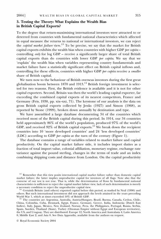
We have assembled a large database documenting 34 of the countries whichreceived most of the British capital during this period. In 1914, our 34 countriesheld approximately 86% of the world’s population, produced 97% of the world’sGDP, and received 92% of British capital exports.15 We break down the recipientcountries into 10 ‘more developed countries’ and 24 ‘less developed countries’(LDC) according to GDP per capita at the turn of the century (Figure 1).

The database contains a range of variables related to market failure and capitalproductivity. On the capital market failure side, it includes import duties as afraction of total import value, colonial affiliation, monetary regime, exchange ratevariance against the pound sterling, changes in the terms of trade and an indexcombining shipping costs and distance from London. On the capital productivity

13 Remember that this view posits international capital market failure rather than domestic capitalmarket failure; the latter implies unproductive capital for investors of all flags. Note also that theconverse of our test is not true. That is, while the determination of flows by fundamental nationalcharacteristics is sufficient to reject the capital market failure view, lack of such determination is merelya necessary condition to reject the unproductive capital view.

14 Certainly Britain (and others) exported capital before this period, as studied by Neal (1990) andothers. But such international investment did not approach the levels attained in the years precedingWorld War 1, which at times exceeded 10% of British GDP.

15 The countries are Argentina, Australia, Austria-Hungary, Brazil, Burma, Canada, Ceylon, Chile,China, Colombia, Cuba, Denmark, Egypt, France, Germany, Greece, India, Indonesia (Dutch EastIndies), Italy, Japan, Mexico, New Zealand, Norway, Peru, the Philippines, Portugal, Russia, Serbia,Spain, Sweden, Thailand (Siam), Turkey (Ottoman Empire without Egypt and European territories),the US, and Uruguay. They are distributed: Europe 12; North America and Australasia 4; Latin America8; Middle East 2; and Asia 8. See Data Appendix, available from the authors on request.



side, it includes the youth dependency ratio, net immigration rates, primary schoolenrolment rates,16 urbanisation, and indices of natural resource abundance madepopular by Sachs and Warner (2000). The data are summarised in Table 3.

Each data point represents one country in one year. For the purposes of trackingchanges in the determinants of flows over time, the observations are sometimesclassified as belonging to one of six time periods delineated in Figure 2. Sixperiods were chosen to utilise local minima as divisions between successive waves ofoutflows. Economists since Hobson (1914, pp. 142–9) have divided pre-war Britishcapital exports into three periods, separated by two large troughs. The first cor-responds to a depression in the aftermath of the Franco-Prussian war and a seriesof defaults in 1874, and the second to economic collapse in Argentina, Australia,and elsewhere in 1890–1. We exploit minor local minima to achieve a slightlyhigher resolution. We discard the first five years of Stone’s flow data (1865–9) dueto limitations in the availability of regressor data before 1870.

Unlike most studies of British capital exports,17 ours focuses exclusively on whatpulled British capital into some countries versus others, rather than what pushed itout of Great Britain. Our dependent variable is therefore the value of total British

GDP per capita,1990 US$, Average 1894–1901

Uni

ted

Kin

gdom

Aus

tral

ia

New

Zea

land

Uni

ted

Stat

es

Uru

guay

Ger

man

y

Fran

ce

Den

mar

k

Arg

entin

a

Can

ada

Swed

en

Spai

n

Cub

a

Chi

le

Nor

way

Ital

y

Aus

tria

-Hun

gary

Port

ugal

Japa

n

Tur

key

Mex

ico

Rus

sia

Phili

ppin

es

Col

ombi

a

Serb

ia

Tha

iland

Bra

zil

Gre

ece

Peru

Indo

nesi

a

Bur

ma

Cey

lon

Chi

na

Indi

a

Egy

pt

0

1,000

2,000

3,000

4,000

5,000

More Developed Countries

Less Developed Countries

Fig. 1. Definition of ‘Less Developed Country’ (LDC). For the purposes of this study, it isassumed that any country with a GDP/capita in 1990 US$ below $2,000 in Period IV –that is, 1894–1901, or roughly the middle of the period under investigation – is an LDC

Sources: See Data Appendix

16 Estimates of the educational attainment of the work force is unavailable for almost all of thecountries in our sample but we use enrollment rates among the school-aged fifteen years previously as aproxy for the current schooling stock per capita.

17 Such as Edelstein (1982) and Davis and Huttenback (1988).



capital exported to a given country during a given period as a fraction of all Britishcapital exported during that period. Push effects are thus entirely eliminated.Scale effects from market size are eliminated by the inclusion of log GDP on theright hand side.18

3.1. The Determinants of Capital Destination

Our central result, presented in Tables 4 to 7, is that the wealth bias was alive andwell during the latter half of the period 1870–1913, and that it can be explained ina way that is sufficient to reject the global capital market failure view. We stress that

Table 3

Summarising the Data

Variable Observations Mean Std. Dev. Minimum Maximum

Share of all British capital 1,700 0.0294 0.0607 0 0.501Share to governments 1,700 0.0294 0.0769 0 0.725Share to private sector 1,700 0.0294 0.0757 0 0.686ln GDP 1,700 23.2 1.54 19.7 27.0LDC dummy 1,700 0.706 0.456 0 1Warfare dummy 1,700 0.0494 0.217 0 1Bond spread over Consol 1,161 0.0344 0.0560 )0.000345 0.484British colony dummy 1,700 0.217 0.412 0 1Gold Standard dummy 1,495 0.483 0.500 0 1Import duties over imports 1,700 0.158 0.110 0.0250 0.582Lagged change in Terms of Trade 1,666 )0.00231 0.156 )1.93 1.23Effective distance to London 1,700 0.372 0.295 0.0102 1.41Population growth 1,666 1.44 1.25 )5.39 13.0Lagged net immigration 1,700 0.504 1.92 )3 3Primary product exports 1,700 0.876 0.177 0.240 1.00Lagged schooling 1,700 0.184 0.162 0.00113 0.579Urbanisation 1,700 0.0903 0.0738 0 0.444

‘ln GDP’ is in 1990 US$. ‘Warfare’ takes the value of 1 if the country is involved in an inter-state war in which Great Britain was not a combatant in that year. ‘Bond spread’ is thedifference between the yield on sovereign bonds in that country and the yield on BritishConsols, in units of percent divided by 100. ‘Import duties over imports’ (‘tariffs’) are allimport duties collected divided by the value of all imports (dutiable or otherwise). ‘Laggedchange in Terms of Trade’ is the once-lagged year-on-year percent change in a Terms ofTrade index, divided by 100. ‘Effective distance’ is the pre-Panama Canal, post-Suez Canalshipping distance in tens of thousands of nautical miles between London and the principalport of the destination country multiplied by a world-wide time-series index of shippingcosts where the year 1869 ¼ 1.00. ‘Population growth’ is the year-on-year change in totalpopulation, in percent. ‘Lagged net immigration’ is an index of net immigration relativeto recipient country population, where 3 represents heavy immigration and )3 representsheavy emigration, lagged by 10 years. ‘Primary product exports’ is the fraction of totalexports falling into categories 0, 1, 2, 3, 4, and 68 of the United Nations Standard Inter-national Trade Classification (SITC) Revision 1. ‘Lagged schooling’ is the fraction of thepopulation below the age of 15 that is currently attending primary school, lagged by15 years. Urbanisation is the fraction of the population living in agglomerations of 100,000or more.

18 Arguably it is more correct to include share of world GDP rather than simply GDP. To the degreethat period-to-period change in world GDP is small, however, this would not be substantially differentfrom simply changing the units on GDP. Making this adjustment to Table 4 (results not reported) doesnot materially alter its conclusions.



we are not asking, as many others have,19 whether perfect global capital marketsexisted during this period. Instead, we are asking whether global capital marketfailure can be viewed as a primary explanation for the wealth bias.

3.1.1. Identifying the fundamentals that matteredIn Table 4, note the significant, negative effect of the LDC dummy on flows whenthat variable is accompanied only by log GDP in regression (1) to (4). This is onemanifestation of the wealth bias. Regression (2) uses a tobit specification to ac-count for the fact that gross capital flows were censored at zero in 14.5% of thecountry-years in question. Regressions (3) and (4) retain the specification of (2)but hold the sample constant with respect the regressions directly below each.

The inclusion of proxies for global market failure and for fundamental nationalcharacteristics in regression (5) and (6) reverses the sign on the LDC indicatorvariable. In other words, after accounting for the effects of other variables, poorcountries received a larger share of British capital than did rich countries in theyears leading up to World War 1.

Which country characteristics are responsible for the change in sign of the LDCdummy? Regression (7) includes the British colony dummy, the Gold Standarddummy, tariffs, terms of trade and effective distance. The sign on the LDC dummyis negative once again, suggesting that the included variables cannot explain

Period I:1870-7

Period II:1878-85

Period III:1886-93

Period IV:1894-1901

Period V:1902-6

Period VI:1907-13

0

20

40

60

80

100

120

140

160

180

200

1865 1870 1875 1880 1885 1890 1895 1900 1905 1910

Mill

ions

of

curr

ent

Pou

nds

Ster

ling

Fig. 2. Division of Pre-WW1 British Capital Exports into Six Time PeriodsSource: Stone (1999)

19 Including Bordo et al. (1999), among many.



wealth bias. Regression (8) includes population growth, immigration, naturalresource endowment, schooling, and urbanisation. Now the sign on the LDCdummy is positive, suggesting that these variables are able to explain wealth bias.

Table 5 asks which of the various country characteristics mattered most. The aimof the Table is to calculate standardised coefficients for regression (2) and (6) inTable 4, allowing us to compare the magnitudes of the effects across differentregressors. The exercise is complicated, however, by a few factors. First, as

Table 4

Explaining Wealth Bias, 1870–1913Dependent variable: Gross British capital flow to country inquestion in year in question as a fraction of total gross Britishcapital flows in that year. All regressions include time period

dummy variables for periods I–V as well as a constant term

Regression number (1) OLS (2) Tobit (3) Tobit (4) Tobit

ln GDP 0.014 0.016 0.016 0.016(8.74)*** (11.08)*** (11.08)*** (11.58)***

LDC dummy )0.040 )0.043 )0.043 )0.037(9.08)*** (9.70)*** (9.70)*** (8.44)***

Adjusted R2 0.170

Regression number (5) OLS (6) Tobit (7) Tobit (8) Tobit

ln GDP 0.025 0.027 0.023 0.027(12.96)*** (18.26)*** (14.49)*** (19.08)***

LDC dummy 0.041 0.049 )0.028 0.038(6.24)*** (6.54)*** (5.74)*** (5.25)**

Warfare 0.007 0.004 )0.007 )0.002(0.85) (0.50) (0.69) (0.28)

Bond spread 0.057 )0.006 )0.157 )0.096(2.14)** (0.14) (3.40)*** (2.46)**

British colony dummy 0.015 0.020 0.037(2.64)*** (3.32)*** (6.13)***

Gold standard dummy 0.016 0.019 0.018(3.73)*** (4.18)*** (3.40)***

Import duties over imports 0.033 0.042 0.224(2.06)** (1.92)* (10.80)***

Lagged change in terms of trade 0.019 0.020 0.020(1.42) (1.15) (1.00)

Effective distance from London )0.027 )0.035 0.036(2.77)*** (3.48)*** (3.86)***

Population growth rate 0.013 0.015 0.014(4.89)*** (6.63)*** (6.82)***

Lagged net immigration 0.011 0.014 0.012(8.87)*** (9.82)*** (9.64)***

Primary product exports 0.153 0.144 0.160(11.15)*** (9.70)*** (11.32)***

Lagged schooling 0.203 0.203 0.198(8.61)*** (10.01)*** (9.53)***

Urbanisation 0.157 0.158 0.141(3.86)*** (4.36)*** (3.99)***

Observations (of which censored) 1,054 1,054 (153) 1,054 (153) 1,138 (163)Adjusted R2 0.466

Absolute values of t statistics in parentheses (robust in column (1)). *significant at 10%;**significant at 5%; ***significant at 1%.



Tab

le5

Com

pari

ng

the

Mag

nit

ude

sof

Dif

fere

nt

Eff

ects

inT

able

4,

Reg

ress

ion

s(2

)an

d(6

)

Du

mm

ies

trea

ted

as:

(1)

(2)

(3)

(4)

(7)

(8)

Mar

gin

alef

fect

sd

eco

mp

osi

tio

n

(5)

Std

.D

ev.

Co

nd

itio

nal

on

y>

0

(6)

Std

.D

ev.

un

con

dit

ion

al

Stan

dar

dis

edco

effi

cien

ts

@Eðyjy

>0Þ=@

x@

Pðy

>0Þ=@

x

fro

m(1

)fr

om

(3)

Con

tin

uou

s[D

iscr

ete]�

Con

tin

uou

s[D

iscr

ete]�

Dep

end

ent

vari

able

0.07

20.

069

Reg

ress

ion

(2)

fro

mT

able

4ln

GD

P**

*0.

008

0.08

21.

576

1.56

70.

165

0.12

8L

DC

du

mm

y***

)0.

021

[)0.

021]

)0.

221

[)0.

213]

0.49

40.

493

)0.

140

)0.

109

Reg

ress

ion

(6)

fro

mT

able

4ln

GD

P**

*0.

014

0.16

61.

576

1.56

70.

305

0.26

0L

DC

du

mm

y***

0.02

5[0

.024

]0.

300

[0.3

07]

0.49

40.

493

0.17

30.

148

War

fare

0.00

2[0

.002

]0.

026

[0.0

26]

0.19

60.

207

0.00

60.

005

Bo

nd

spre

ad)

0.00

3)

0.03

50.

048

0.05

8)

0.00

2)

0.00

2B

riti

shco

lon

y***

0.01

0[0

.011

]0.

120

[0.1

12]

0.42

90.

412

0.06

00.

049

Go

ldst

and

ard

***

0.01

0[0

.010

]0.

117

[0.1

18]

0.49

10.

493

0.06

70.

057

Tar

iffs

*0.

022

0.25

80.

115

0.11

60.

035

0.03

0T

erm

so

fT

rad

e0.

010

0.12

20.

097

0.10

20.

014

0.01

2E

ffec

tive

Dis

tan

ce**

*)

0.01

8)

0.21

20.

275

0.28

2)

0.06

8)

0.06

0P

op

ula

tio

ngr

ow

th**

*0.

008

0.08

91.

111

1.07

90.

115

0.09

6N

etim

mig

rati

on

***

0.00

70.

083

1.97

61.

977

0.19

10.

164

Pri

mar

yp

rod

.ex

po

rts*

**0.

075

0.88

30.

200

0.19

50.

206

0.17

3Sc

ho

oli

ng*

**0.

105

1.24

30.

173

0.16

80.

250

0.20

8U

rban

isat

ion

***

0.08

10.

964

0.07

50.

073

0.08

50.

071

Sam

ple

ish

eld

con

stan

tth

rou

gho

ut

Tab

le.

Ino

rigi

nal

regr

essi

on

:*s

ign

ifica

nt

at10

%;

**si

gnifi

can

tat

5%;

***s

ign

ifica

nt

at1%

.�F

or

du

mm

yva

riab

les,

the

dis

cret

em

argi

nal

effe

ctsh

ow

nin

colu

mn

(2)

and

(4)

rep

rese

nts

chan

geas

soci

ated

wit

ha

dis

cret

ech

ange

fro

m0

to1

inth

ein

dep

end

ent

vari

able

.C

olu

mn

(7)

isth

eco

effi

cien

tfr

om

colu

mn

(1)

mu

ltip

lied

by

the

con

dit

ion

alst

and

ard

dev

iati

on

of

the

ind

epen

den

tva

riab

lein

colu

mn

(5)

div

ided

by

the

con

dit

ion

alst

and

ard

dev

iati

on

of

the

dep

end

ent

vari

able

atth

eto

po

fco

lum

n(5

).T

his

rep

rese

nts

the

nu

mb

ero

fst

and

ard

dev

iati

on

so

fch

ange

inth

ed

epen

den

tva

riab

leas

soci

ated

wit

ha

on

est

and

ard

dev

iati

on

chan

gein

the

ind

epen

den

tva

riab

le.C

olu

mn

(8)

isth

eco

effi

cien

tfr

om

colu

mn

(3)

mu

ltip

lied

by

the

un

con

dit

ion

alst

and

ard

dev

iati

on

of

the

ind

epen

den

tva

riab

lein

colu

mn

(6).

Th

isre

pre

sen

tsth

en

um

eric

alch

ange

inth

ep

rob

abil

ity

of

bei

ng

un

cen

sore

dd

ue

toa

on

est

and

ard

dev

iati

on

chan

gein

the

ind

epen

den

tva

riab

le.



Tab

le6

Dec

ompo

sin

gT

able

4,

Reg

ress

ion

s(2

)an

d(6

)A

cros

sT

ime

Est

imat

or:

Tob

it.

Dep

end

ent

vari

able

:G

ross

Bri

tish

cap

ital

flo

wto

cou

ntr

yin

qu

esti

on

inye

arin

qu

esti

on

asa

frac

tio

no

fto

tal

gro

ssB

riti

shca

pit

alfl

ow

sin

that

year

(1)

All

per

iod

s(2

)P

erio

dI

(3)

Per

iod

II(4

)P

erio

dII

I(5

)P

erio

dIV

(6)

Per

iod

V(7

)P

erio

dV

I

lnG

DP

0.01

60.

017

0.01

30.

011

0.02

00.

020

0.01

7(1

1.08

)***

(5.0

7)**

*(3

.57)

***

(3.2

9)**

*(6

.24)

***

(4.2

6)**

*(5

.32)

***

LD

Cd

um

my

)0.

043

)0.

026

)0.

059

)0.

053

)0.

035

)0.

036

)0.

044

(9.7

0)**

*(2

.42)

**(5

.25)

***

(5.0

9)**

*(3

.62)

***

(2.5

9)**

(4.6

5)**

*(8

)A

llp

erio

ds

(9)

Per

iod

I(1

0)P

erio

dII

(11)

Per

iod

III

(12)

Per

iod

IV(1

3)P

erio

dV

(14)

Per

iod

VI

lnG

DP

0.02

70.

028

0.02

70.

025

0.03

50.

036

0.03

3(1

8.26

)***

(4.7

7)**

*(6

.99)

***

(8.2

9)**

*(1

1.24

)***

(8.2

6)**

*(1

4.17

)***

LD

Cd

um

my

0.04

9)

0.00

50.

080

0.03

20.

068

0.12

40.

076

(6.5

4)**

*(0

.21)

(4.2

3)**

*(2

.23)

**(4

.53)

***

(4.9

5)**

*(5

.29)

***

War

fare

0.00

40.

012

)0.

002

)0.

018

)0.

043

0.03

30.

016

(0.5

0)(0

.54)

(0.1

2)(0

.38)

(2.3

5)**

(1.0

8)(1

.32)

Bo

nd

spre

ad)

0.00

6)

0.07

1)

0.03

90.

085

0.36

00.

718

0.85

8(0

.14)

(0.8

2)(0

.50)

(1.0

9)(2

.73)

***

(2.7

5)**

*(3

.06)

***

Bri

tish

colo

ny

du

mm

y0.

020

0.04

50.

019

0.00

10.

030

)0.

039

0.00

2(3

.32)

***

(2.2

3)**

(1.2

9)(0

.09)

(2.4

6)**

(2.1

2)**

(0.2

0)G

old

stan

dar

dd

um

my

0.01

90.

002

0.04

2)

0.00

00.

032

0.06

10.

023

(4.1

8)**

*(0

.16)

(3.4

3)**

*(0

.02)

(2.9

5)**

*(4

.20)

***

(2.7

6)**

*Im

po

rtd

uti

eso

ver

imp

ort

s0.

042

0.21

2)

0.03

7)

0.06

5)

0.12

9)

0.16

2)

0.08

1(1

.92)

*(3

.50)

***

(0.6

3)(1

.47)

(2.4

0)**

(2.1

5)**

(1.7

5)*

Lag

ged

chan

gein

Ter

ms

of

trad

e0.

020

0.01

9)

0.03

40.

031

0.01

1)

0.00

10.

045

(1.1

5)(0

.39)

(0.6

7)(0

.94)

(0.3

8)(0

.02)

(1.5

8)E

ffec

tive

dis

tan

cefr

om

Lo

nd

on

)0.

035

)0.

017

)0.

043

)0.

038

)0.

049

)0.

057

)0.

144

(3.4

8)**

*(0

.80)

(1.7

4)*

(1.3

6)(1

.84)

*(1

.33)

(7.9

0)**

*P

op

ula

tio

ngr

ow

thra

te0.

015

)0.

002

0.04

20.

026

0.01

10.

024

0.01

7(6

.63)

***

(0.3

6)(6

.12)

***

(5.1

5)**

*(1

.87)

*(2

.80)

***

(3.7

3)**

*L

agge

dn

etim

mig

rati

on

0.01

40.

012

0.01

40.

020

0.01

20.

021

0.01

8(9

.82)

***

(2.5

9)**

(3.2

8)**

*(6

.40)

***

(4.3

6)**

*(5

.05)

***

(8.6

8)**

*P

rim

ary

pro

du

ctex

po

rts

0.14

40.

059

0.14

90.

173

0.20

80.

261

0.24

4(9

.70)

***

(1.4

2)(4

.56)

***

(5.6

1)**

*(6

.27)

***

(5.3

0)**

*(9

.50)

***

Lag

ged

sch

oo

lin

g0.

203

0.05

40.

275

0.23

50.

191

0.38

20.

294

(10.

01)*

**(0

.73)

(4.8

5)**

*(5

.42)

***

(4.7

2)**

*(6

.74)

***

(8.8

9)**

*U

rban

isat

ion

0.15

8)

0.13

20.

160

0.07

20.

373

0.09

10.

112

(4.3

6)**

*(0

.89)

(1.8

7)*

(0.9

4)(4

.85)

***

(0.7

2)(1

.88)

*O

bse

rvat

ion

s(o

fw

hic

hce

nso

red

)1,

054

(153

)17

2(3

2)19

1(2

9)19

6(3

3)19

6(3

2)12

9(1

8)17

0(9

)

Ab

solu

teva

lue

of

tst

atis

tics

inp

aren

thes

es.

*sig

nifi

can

tat

10%

;**

sign

ifica

nt

at5%

;**

*sig

nifi

can

tat

1%.

All

regr

essi

on

sin

clu

de

aco

nst

ant

term

(no

tre

po

rted

).



McDonald and Moffit (1980) point out, the tobit coefficients reported in Table 4represent an amalgam of two effects: the marginal effect of a change in theregressor on the value of the regressand conditional on the latter being uncen-sored and the marginal effect on the probability that the observation is censored.Both of these may be of interest. Second, we must treat dummy variables as con-tinuous in order to make a meaningful comparison of standardised marginal

Table 7

Determinants of Bond Yield Spreads and of Lendingto the Public versus Private Sector

Dependent variable(2) Tobit (4) TobitPublic sector� Private sector�

ln GDP 0.012 0.022(2.96)*** (12.30)***

LDC dummy )0.052 )0.060(4.07)*** (10.62)***

Dependent variable (1) OLS (3) Tobit (5) TobitBond spread Public sector� Private sector�

ln GDP 0.018 0.040(3.73)*** (22.04)***

LDC dummy 0.060 0.059(2.35)** (6.45)***

Warfare 0.041 )0.014(1.43) (1.28)

Bond spread )0.975 0.056(3.80)*** (1.14)

British colony dummy )0.031 0.074 0.003(6.18)*** (4.00)*** (0.42)

Gold standard dummy )0.012 0.036 0.018(4.23)*** (2.37)** (3.24)***

Tariffs 0.124 )0.113 0.094(4.58)*** (1.43) (3.54)***

Lagged change in Terms of Trade )0.013 0.086 0.006(0.84) (1.53) (0.27)

Effective distance 0.069 0.011 )0.069(5.53)*** (0.35) (5.60)***

Population growth rate )0.006 0.011 0.021(4.00)*** (1.67)* (7.89)***

Lagged net immigration )0.002 0.021 0.019(2.39)** (4.47)*** (11.57)***

Primary product exports 0.009 0.153 0.218(1.10) (2.94)*** (12.12)***

Lagged schooling )0.021 0.027 0.320(2.54)** (0.41) (13.17)***

Urbanisation )0.093 0.335 0.082(4.22)*** (2.96)*** (1.89)*

Observations (of which censored) 1,054 1,054 (405) 1,054 (196)R2 0.297

Absolute value of t statistics in parentheses (robust in column (1)). *significant at 10%; **significant at5%; ***significant at 1%. �‘Public sector’ signifies that the dependent variable is the gross flow of Britishcapital to government borrowers in the country and year in question as a share of all British capitalgoing to government borrowers in that year. �‘Private sector’ signifies that the dependent variable is thegross flow of British capital to private sector borrowers in the country and year in question as a share ofall British capital going to private sector borrowers in that year.



effects across regressors but the marginal effects of discrete changes in the dummyvariables may also be of interest and are therefore reported in the Table.

Columns (1) and (2) of Table 5 show the marginal effect of a unit change in theunderlying regressor on the dependent variable (share of all British capital exportsin each year received by the country in question) conditional on the observationbeing uncensored. That is, this is the effect of the regressor on capital flows inthose countries that received strictly positive flows. Column (3) and (4) show themarginal effect of a unit change in the underlying regressor on the censoringprobability, the probability that a country received no British capital in a givenyear. Column (5) and (6) report the standard deviation of the underlyingregressors, conditional on uncensored and unconditional, respectively. Columns(7) and (8) report standardised coefficients from columns (1) and (3). Column(7) reports the number of standard deviations of change in the dependent variablethat are associated with a one standard deviation change in the regressor, allconditional on the observation being uncensored. Column (8) reports the nu-meric change in censoring probability associated with a one standard deviationchange in the regressor (unconditional).

Table 5 contains two key lessons. The first is the exact degree of wealth bias andthe degree to which it is explained in this analysis. Column (2) shows that amongthose countries that received positive capital flows, controlling only for the size ofthe economy the typical less developed country received a share of British capitalthat was smaller by 2.1% of total capital exports than the share received by a typicalrich country – an enormous difference in a world where the average share was 2.9%of total capital exports.20 After controlling for country characteristics, however, thetypical LDC received a share of British capital that was 2.4% larger than the typicalrich-country share. Column (4) shows that controlling only for size of the economy,LDCs were 21.3% more likely to receive zero British capital. After controlling forcountry characteristics, LDCs were 30.7% less likely to receive zero capital.

The second lesson is that certain country characteristics mattered much morethan others in determining capital flows. The standardised coefficients of column(7) show that schooling, natural resource endowment, demographic structure,immigration and urbanisation dominate the explanatory power of British colony,Gold Standard, tariffs, terms of trade shocks and effective distance.21 Capital flowsare almost eight times as sensitive to the former group of variables as a whole asthey were to the latter group as a whole.

Table 6 shows that these findings are robust to disaggregation across timeperiods. The Table decomposes regression (2) and (6) from Table 4 into sixsubsamples according to the time periods delineated in Figure 2. Regression (1)and (8) in Table 6 simply replicate regression (2) and (6) from Table 4. Regres-

20 The share of a typical country in any year when there are 34 recipient countries is 1/34, or 2.94%.This must always be true given how our share variable is constructed, and is the reason why very differenttypes of capital flow share variables have the same mean in Table 3.

21 Effective distance from London is calculated as the physical distance of the shortest availableshipping route between London and the closest principal port of the country in question (pre-PanamaCanal, post-Suez Canal) multiplied by an index of transoceanic shipping costs. See Data Appendix fordetails, available from the authors on request.



sions (2) to (7) in Table 6 show that wealth bias was quite consistent across time,and regressions (9) to (14) show that the added regressors can explain wealth biasin every period except period I. In general, schooling, natural resource endow-ment, demographic structure, immigration, and urbanisation matter more in eachperiod and matter more consistently across periods. The positive effect of tariffsappears confined to the first period. The sample is held constant between vertic-ally-paired regressions.

3.1.2. Rejecting the global capital market failure view of the wealth biasThe evidence in Tables 4 to 6 is consistent with the predictions of the unpro-ductive domestic capital view of the wealth bias but not with those of the globalcapital market failure view. The global capital market failure view predicts thatinvolvement in warfare should have choked off British capital inflows, that coun-tries with a higher sovereign bond spread should have received a smaller share ofBritish capital and that country fundamentals unrelated to creditworthiness shouldnot have affected inflows. In fact, country fundamentals were the best determi-nants of flows and overpower the effects of warfare and bond spreads. It cannot besaid that the global capital market failure view is totally without merit; after all,bond spread, British colony, the Gold Standard, terms of trade shocks and effectivedistance from London all have the predicted signs. However, the market failureview pales in importance compared with the competing unproductive domesticcapital view.

How can we be sure that the ‘fundamentals’ are not proxies for creditworthi-ness? Could natural resource endowment or education have made a recipientcountry more creditworthy in the eyes of British investors, rather than directlyaffecting the return to capital? Regression (1) in Table 7 explores this issue. Thedependent variable is the spread between the yield on sovereign bonds in 27countries and the yield on the riskless British Consol. The results are consistentwith the premise that the bond spread captures investment risk: British coloniesand those on the Gold Standard had lower spreads, while highly protectedcountries far from London had higher spreads. Natural resource endowment didnot affect bond spread in a statistically significant way, although schooling, pop-ulation growth and immigration were statistically significant predictors of lowerbond spreads. Recall from Table 4, however, that even after accounting for theeffect of these latter three variables on creditworthiness (by including bond spreadas a regressor), they remain some of the top determinants of capital flows. It is forthis reason that we describe them along with natural resource endowment as‘fundamentals’, or factors that affect capital flows through their effect on thereturn to domestic capital.

Just because the predictors of bond spread have the ‘right’ sign does not, ofcourse, prove unambiguously that bond spreads capture creditworthiness. In thetransition from autarky (around 1870) to integrated world capital markets(around 1913), bond spreads would have had very different meaning: bondspreads would have attracted capital at the start, while at the end they shouldhave been an indicator of risk, thus deterring foreign capital. Figure 3 reveals amassive global convergence in bond spreads in the years leading up to World



War 1, a phenomenon discussed elsewhere (Mauro et al., 2002). Not only doesthe mean of these spreads fall from 4.07% to 1.65% between periods III and VIbut the coefficient of variation also falls from 1.75 to 1.07. We interpret thisevidence as support for the view that bond spreads were increasingly an indi-cator of creditworthiness.

Period average spread between government bond yieldsand yield on UK consol, in %, 27countries, Periods I through VI

0

5

10

15

20

25

30

35

40

1870 1875 1880 1885 1890 1895 1900 1905 1910 1915

ArgentinaAustraliaAustria-HungaryBrazilCanadaCeylonChileChinaColombiaDenmarkEgyptFranceGermanyGreeceIndiaItalyJapanMexicoNew ZealandNorwayPeruPortugalRussiaSpainSwedenTurkeyUnited StatesUruguay

Fig. 3. Convergence in Sovereign Bond Yields During the First Global Capital Export BoomSource: Taylor (2000)



3.1.3. SpecificationOur conclusions are robust to several changes of regression specification.Regressions (7) and (8) in Table 4 show that the sign change on LDC betweenregressions (2) and (6) does not spring from a paucity in degrees of freedom.Inclusion of just a few of the variables associated with the unproductive domesticcapital view largely reproduces the results of regression (6), while inclusion of thesame number of variables related to the global capital market failure view cannotexplain the wealth bias.22

3.1.4. Endogeneity biasWe have treated immigration as exogenous to capital flows and to the other fun-damentals of the right-hand side. That certainly would have been so if European‘push’ conditions dominated. But a rich literature makes it clear that the massmigrations were also determined by ‘pull’ in receiving regions (Hatton and Will-iamson, 1998). Since we are uncertain about whether push or pull dominated, werun all regressions using lagged immigration, defined as average net immigrationlagged by ten years.

We have also treated education and natural resource endowment as exogenous.We are sympathetic to any argument suggesting that British investment may haveraised the returns to education in recipient countries. Note, however, that oureducation regressor is lagged by 15 years. We also agree that British investmentcontributed to the development of natural resources in the recipient countries.But regressing period VI capital flows on period I natural resource endowmentdoes not alter the status of this variable as a primary determinant of capital flows.This is not a surprise, since less than 10% of British capital exports were investeddirectly in projects to extract natural resources such as metals, nitrates, oil, tea,coffee, and rubber (Stone, 1999). The vast majority of British capital went torailroads and other transportation infrastructure, financial institutions, factoriesand communications infrastructure.

3.1.5. Influential observationsMajor recipients of British capital included the US, Argentina, Australia, andCanada. Was one of these countries largely responsible for the results in Tables 4to 7? Additionally, it is not known how much British investment in ‘China’ wasactually investment in resource-poor Hong Kong. Would the elimination of Chinaalter the results? The following are the standardised marginal effects on Britishcapital share with respect to the LDC dummy from column (7) of Table 5 whenvarious countries are omitted from the sample: Argentina, 0.240; Australia, 0.144;Canada, 0.175; China 0.141; US, 0.120 (whole sample: 0.173). The standardised

22 Neither do several other changes of specification, not reported here, alter our results. OLS crosssection regressions on averages across each of the six periods retain the ability of fundamentals toexplain wealth bias. A version of Table 6 that includes country random effects and a correction for serialcorrelation retains the ability of country fundamentals to explain wealth bias in all but one of theperiods where it is explained by Table 6 (period III). Including exchange rate variance or an indicatorof Gold, Silver or Bimetallic standard instead of just the Gold Standard; including variance in Terms ofTrade instead of cumulative change in Terms of Trade; or defining ‘LDC’ according to relative PPP-adjusted real wage levels do not materially alter the results.



coefficient on natural resource endowment when China is omitted is 0.235 (wholesample: 0.206). In all cases the underlying coefficient estimates remain statisticallysignificant at the 1% level. In short, none of these countries by itself can be drivingthe ability of fundamentals to explain wealth bias.

3.1.6. Selection biasWe have implicitly assumed that if borrowing countries have some preference forthe nationality of their creditors, it is uncorrelated with the borrower traits we haveincluded as regressors. For example, it could be that the reason we observe moreBritish capital going to better-educated countries is because less-educated countriestended to borrow in Berlin or Paris. While we are not aware of comparable data onGerman and French capital flows to test this hypothesis directly, we are highlysceptical of its relevance. First, the most natural dimension for self-selection,colonial affiliation, has far less importance than other determinants of flows. Sec-ond, Table 1 shows that the fraction of French and German capital going toWestern Europe – where schooling and urbanisation were high – was much greaterthan the corresponding figure for Britain. Third, Britain provided roughly half theworld supply of international capital during the period in question (Obstfeld andTaylor, 2003), a dominance capable of constraining borrower self-selection. Fourth,while it is reasonable that resource-poor or human capital-poor countries mightrequire more sophisticated financial instruments to hedge against risk, no countrycompeted successfully with British financial technology at this time.

3.1.7. Global capital market deepening and transitions through timeTable 6 documents an upward drift in the share of British capital flows explained,and, furthermore, that the fundamentals exhibit a stronger impact as the decadesunfold.23 What made flows respond to fundamentals after 1890s more than theyhad previously? Figures 2 and 3 suggest that the international capital market wassimply deeper than it had been before24 as British capital spread to a wider areathan ever before – including major movements to Brazil, Mexico, Chile, Egypt,South Africa, India, Russia, and the Far East (Hobson, 1914, pp. 157–8). Feis(1930, pp. 12–3) puts it thus:

Changing political relations took British capital into countries from which ithad previously abstained – Japan [Alliance of 1902], Russia [Anglo-Russianagreement, 1907], and Turkey. But more important than these causes in

23 This shift is statistically significant. We include a dummy variable for periods IV, V and VI, as well asinteraction terms between this dummy and the explanatory variables from British colony to urbanisa-tion. A positive and significant interaction term is interpreted as signifying an increase in the coefficientvalue between periods I–III and periods IV–VI. Omitting period I, a Chow test fails to reject that all theinteraction terms are jointly equal to zero for British colony, Gold Standard, tariffs, terms of trade, andeffective distance (F(5, 856) ¼ 0.56, p-value 0.731). A similar Chow test rejects the hypothesis that theinteraction terms are jointly zero for ‘fundamentals’ population growth, immigration, primary productexports, schooling and urbanisation (F(5, 856) ¼ 6.02, p-value < 0.0005). Including period I, the re-spective statistics are F(5, 1028) ¼ 2.22 (p-value 0.0503) and F(5, 1028) ¼ 2.17 (p-value 0.0549). Inother words, from periods II and III (1878–93) to periods IV–VI (1894–1913) there was a statisticallysignificant increase in the explanatory power of the ‘fundamentals’ but not in the other regressors.

24 Only about 40% of British capital exports that occurred during 1870–1914 flowed overseas before1895.



producing a great growth in foreign investment was the fact that during the1900–1914 period those distant lands to which the capital had been goingin earlier periods, seemed to have overcome the risks and crashes of theirfirst growth. Now in the greater stability and greater order of their devel-opment, they needed still more capital than before and offered surer re-turn. Or – the idea presents itself in alternative form – it was as though manyregions of the world in which British capital had invested itself had come tofit themselves better for the investment, learning from pioneer failures.

Gallman and Davis (2001, Ch. 7) provide extensive evidence of ‘financialdeepening’ in British capital recipient countries during this period, includingrising measures of total financial assets and assets of financial intermediaries as afraction of GNP.

There may, of course, be other reasons why the fundamentals exhibit anincreasingly powerful influence through time. Economic historians have long ar-gued that conventional physical capital accumulation mattered far more in the19th century, while human capital accumulation mattered far more in the 20thcentury, the changing mode of accumulation driven by the evolution of techno-logies on the demand side and/or by the release of constraints on schoolinginvestment on the supply side. Perhaps the somewhat increasing importance ofhuman capital endowment as a determinant of British capital inflows simply re-flects this transition.

One explanation for the increasing importance of fundamentals over time canbe easily ruled out. If the data on British capital exports included re-investment indebt that was periodically ‘rolled over’, one might expect that a country withfundamentals that attracted capital would build up a larger and larger stock ofdebt over time, thus experiencing ever larger ‘rollover’ inflows of capital. The flowsexplored here do not, however, include debt rollover. Rather, they were compiledto include only ‘new issues’, and only reflect actual financial transfers rather thanaccounting changes (Stone, 1999; Jenks, 1927). Furthermore, a necessary condi-tion for this ‘rollover’ explanation would be to observe long-term persistence inthe geographical distribution of flows. Table 8 shows Spearman’s correlationcoefficient between the rankings of British capital recipients in the six periods;there is very little persistence in the evidence.

3.2. Capital Flows to Governments and to the Private Sector

Disaggregating capital flows by recipient sector allows us to learn even more abouthow they were determined. Table 9 shows that during most of the pre-war years,British capital exports were primarily invested in the private sector of the desti-nation country. What drove flows to governments and how did these interact withflows to the private sector? Regressions (2) and (3) in Table 7 explore the deter-minants of flows to governments, while regressions (4) and (5) do the same forcapital flows to private sector borrowers. The first item to note is that the wealthbias is alive and well for both types of flows, as is the ability of the includedcovariates to explain it and change the sign on the LDC dummy.



Also noteworthy are certain broad differences between government and privatesector flows. Government flows were more closely associated with British colonies,low bond spreads, Gold Standard participants and highly urbanised countries.Private sector flows were more closely associated with large natural resourceendowments, growing populations and educated populations. That British colo-nial status mattered for government flows is to be expected in light of the highlyunreliable contract enforcement efforts by the British government on behalf ofBritish investors in foreign governments documented by Feis (1930, pp. 98–117).Such interventions were often guided more by British political or territorial aspi-rations than by a sense of duty to its investors and those investors suffered themany defaults catalogued by Lindert and Morton (1989).

Abundant anecdotal evidence suggests that warfare was an important deter-minant of demand for sovereign borrowing, which in itself would make capitalflows to governments unrelated to recipient country characteristics, even withoutinternational market failure. There were massive loans to the French and Germangovernments during the Franco-Prussian War in the 1870s, to the South Africangovernment at the time of the Boer War in the 1890s and to the Japanese gov-ernment to finance its war with Russia just after 1900. In each of these cases, total

Table 9

Percentage of British Capital Exports to 34 Countries, by Recipient Sector

Public Sector Private Sector

Period I 1870–1877 55.4 44.6Period II 1878–1885 42.3 57.7Period III 1886–1893 33.0 67.0Period IV 1894–1901 39.0 61.0Period V 1902–1906 29.6 70.4Period VI 1907–1913 28.1 71.9

Source: Stone (1999).

Table 8

Spearman’s Correlation Coefficient for the Rank Order of the 34 BritishCapital Recipients in Six Periods, by Share of British Capital Received

Period I Period II Period III Period IV Period V Period VI

Period I 1.000 0.039 0.053 )0.024 )0.005 )0.061Period II – 1.000 0.263 0.342 0.099 0.300Period III – – 1.000 0.268 0.108 0.206Period IV – – – 1.000 0.285 0.397Period V – – – – 1.000 0.272Period VI – – – – – 1.000

In each period, all countries were ranked from 1 to 34 according to the share of totalBritish capital exports in that period received by each country, in descending order.The numbers in the Table represent Spearman’s (equivalently Pearson’s) correlationcoefficient between rank orderings in different periods. They are intended as anindicator of period-to-period persistence in the geographic distribution of Britishcapital exports. Periods are defined in Figure 2.



wartime sovereign borrowing dramatically exceeded the cumulative total of allpeacetime borrowing during the five decades that preceded the First World War.Contemporary observers likewise identified warfare as the primary determinant ofsovereign borrowing.

Although warfare is not statistically significant in Table 7, the magnitude of thecoefficient is much larger than in the corresponding regressions with total capitalflows as the dependent variable. Upon decomposing the results of regression (3)in the fashion of Table 5, we observe that the effect of a discrete change in thewarfare dummy on the government flows (conditional on uncensored) was 0.0121,or six times larger than for total capital flows. The effect on probability uncensoredis 0.104, or about four times larger than for total capital flows. The analysis ofSection 2 showed that the global-capital-market-failure view predicts a negativecoefficient on warfare, which we do not observe.

We must be cautious, of course, in drawing a hard and clear line between flowsto governments and flows to the private sector, as Simon, Jenks and Stone definedthem. For one thing, government involvement in many of these ‘private sector’loans tended to be heavy – especially in the case of railroads, the largest category ofprivate sector borrowing. Whether through land grants, subsidies, or loan guar-antees, governments were indirect partners to many private sector investments(Nurkse, 1954, p. 749). Furthermore, when analysing these flows from the per-spective of the 21st century, we must remember that most of these private-sectorflows went to investments in what Simon (1968, p. 23) calls ‘social overhead cap-ital’. These included projects with significant positive externalities – like railroadsand public utilities – projects often undertaken today by government borrowers.

3.3. Investment in Governments Crowded-in Private Investment

Table 10 suggests that previous investment in governments ‘crowded in’ subse-quent private sector investment. Capital flow data in this Table were divided into

Table 10

Evidence that Investment in the Public Sector ‘Crowded In’ Investment in the PrivateSector but not the Other Way Around

Regressand: Current investmentin private sector

Current Investmentin public sector

Estimator:Panel FixedEffects Anderson-Hsiao

PanelFixed Effects Anderson-Hsiao

Regressor:Lagged investment in private sector )0.2393 )0.6698 0.05996 0.05299

(3.670)*** (4.415)*** (1.465) (1.023)Lagged investment in public sector 0.1587 0.4817 )0.3661 0.01493

(1.721)* (3.852)*** (6.320)*** (0.100)Observations 272 238 272 238

Absolute values of t-statistics are in parentheses. *Significant at the 10% level. ***Significant at the 1%level. Data have been divided into ten periods of five years each. Variable values are averages over eachperiod. See text for a description of the particular Anderson-Hsiao estimator used.



ten periods of five years each, over which annual variable values are averaged, and‘lagged’ refers to the five-year period preceding the one in question. Because twolags were necessary for the panel fixed-effects model, the number of observations is(34 countries · 10 periods) ) (34 countries · 2 lags) ¼ 272. Similarly, the Anderson-Hsiao estimator, which uses 3 lags, lowers the number of observations to 238.

The panel fixed-effect estimates reveal a positive effect of lagged public sectorinvestment on current private sector investment (significant at 9%), while theeffect of lagged private sector investment on current public sector investment ismuch smaller and insignificant. It is well known, however, that inclusion of alagged dependent variable in a fixed-effects panel regression can produce severelybiased coefficients, especially for small panels like this one (Nickell, 1981).Anderson and Hsiao (1981) offer a solution by instrumenting for the once-diff-erenced dependent variable with the twice-differenced dependent variable.25 Theresults of this Anderson-Hsiao estimation are also reported in Table 10. Thecrowding-in effect of public sector investment on private is confirmed and againno such causation is seen from private sector investment to public. Note thenegative coefficient for past private investment regressed on current privateinvestment, likely reflecting the fact that in each period private investment wasexpanding into countries that had never received it before. This again illustratesthe deepening of the global capital market over time. Furthermore, it arguesagainst geographic persistence of public (and thus total) investment flows: publicinvestment tended to grow in wartime and shrink in peacetime; it did not pro-gressively expand.

Why did crowding-in take place? One explanation might be that loaning topublic entities contributed to financial deepening: for example, investment in thegovernment debt of South Africa during the Boer War may have opened investors’eyes to private sector opportunities subsequently. Alternatively, private investmentfollowed investment in governments because governments borrowed to make war,and the private sector subsequently borrowed to rebuild the country or to makegood on foregone private accumulation.

4. Discussion and Historiography

The question of whether pre-WWI British capital exports were driven by domesticcapital productivity or by global market failure has been around at least sinceHobson, who was writing at the capital export peak. Hobson raised the questionand then offered as an explanation the declining importance of global marketfailure and thus, presumably, the rising importance of capital productivity fun-damentals (Hobson, 1914, p. xii). Were Hobson alive today, he probably wouldwant to leave his explanation unchanged. After all, the evidence we have presentedsuggests that the largest capital exporter in history was indeed sending its moneywhere it could earn the highest return and that was where the fundamentals servedto raise capital’s productivity.

25 Judson and Owen (1999) use a Monte Carlo approach to demonstrate that the Anderson-Hsiaoestimator essentially eliminates this bias, though it is not as efficient as other methods for small panels.



As Edelstein (1982, p. 7) points out, the idea that third factors like land couldallow for increasing returns to British capital exports in newly-settled regions goesback at least to Adam Smith (1776, pp. 89–93). Feis (1930, pp. 25, 31) also fa-voured third-factor fundamentals by asserting that the ‘British investor was sendinghis capital where there was the growth of youth, and where the land was yieldingriches to the initial application of human labour and technical skill’, undeterredby ‘[s]trong risks, bad climates’ and ‘isolation’. After clearly identifying the wealthbias by stating that ‘income per head in the principal debtor countries of thenineteenth century – the newly settled regions – can never have been far belowEuropean levels’, Nurkse (1954, p. 757) also concludes that capital was attracted‘not to the neediest countries with their ‘‘teeming millions’’’, but rather chasedthe ‘great migration’ to the ‘spacious, fertile, and virtually empty plains’ of certaincountries (pp. 745, 750). Thus, our answer to Hobson’s question is not new.

4.1. Second-Order Determinants of Flows

This paper provides empirical confirmation of the views of pioneer analysts of theglobal capital market and shows that they are superior to competitors. We nowconsider several popular competing explanations of British capital flows which wefind to be of only secondary importance.

4.1.1. Terms of tradeWe can find no evidence supporting the view that capital flows were primarilydriven by recent terms of trade shocks. Thomas (1968, pp. 49–50) felt that‘movements in the terms of trade are to be looked upon more as consequencesthan as causal forces’ of capital flows. ‘Cairncross [1953]’, he writes, ‘has to go outof his way to find reasons why heavy British capital exports in the eighties shouldhave coincided with a deterioration in the terms of trade of the borrowing countries,for the link seemed to work so well in the nineties and the 1900s’. In defence of hiscritique, Thomas expounds a plausible model of causation from capital flows toterms of trade. Our results support his critique (but not necessarily his model).

4.1.2. Colonial statusMany historians have viewed British capital exports as part and parcel of Britishcolonial expansion. This view appears reasonable in light of such developments asthe 1900 revision of the Colonial Stocks Act, which promoted Empire investmentby allowing registered securities in British colonies and dominions to be purchasedby trust bodies and large institutional investors previously banned from foreigninvestment (Feis, 1930, pp. 92–5). Yet, many have criticised this view by simplyciting counter-examples like non-Empire capital flows to Argentina and the US(Simon, 1968, p. 24; Platt, 1986, p. 25). What we add here is multivariate, quan-titative support their univariate, qualitative analysis. Our results leave no doubtwhatsoever that markets mattered far more than flag for private-sector Britishinvestment heading abroad. British colonies did get a larger share of capital flowsto government recipients, but market concern was the first-order determinant ofdestination.



4.1.3. The Gold StandardEichengreen (1996, p. 18) has stated unequivocally that in the 1870s, ‘[i]ndus-trialisation rendered the one country already on gold, Great Britain, the world’sleading economic power and the main source of foreign finance. This encouragedother countries seeking to trade with and import capital from Britain to follow itsexample’. While we also detect a positive and statistically significant effect ofparticipation in the Gold Standard, the magnitude of this effect on investmentflows is much lower than the effects of natural resources, education, demographicstructure and capital scarcity, and somewhat lower than urbanisation.

There are many possible explanations for our finding but the prominent one isthat the effects of economic, demographic and geographic fundamentals simplyoutweighed the effects of the Gold Standard. Bordo and Schwartz (1996, p. 41)find anecdotal evidence that ‘adherence to the rule by Argentina may have hadsome marginal influence on capital calls … before 1890 … but that the keydeterminant was the opening up of the country’s vast resources to economicdevelopment once unification and a modicum of political stability were achieved’.We confirm the Bordo and Schwartz Argentina finding on a global scale: if thefundamentals were not satisfied, going on gold did not bring in the capital. Basedon a sample of nine capital-importing countries, Bordo and Rockoff (1996) arguethat adopting the Gold Standard lowered the costs of borrowing in world capitalmarkets and that it served as a ‘good housekeeping seal of approval’.26 However,Bordo and Rockoff do not control for any economic, demographic or geographicfundamentals. Flandreau et al. (1998) and Obstfeld and Taylor (2003) also find anassociation between lower interest rate spreads and going on gold, but againwithout controlling for a range of determinants of capital productivity. We do notdispute these findings – indeed the coefficient on gold in Table 4 confirms them –but we do suggest that gold was nowhere near the most important determinant offlows.

5. Conclusion

During the first globalisation boom prior to World War I, British capital did not goto poor, labour abundant economies. We call this the wealth bias. The evidencerejects the global-capital-market-failure explanation of the wealth bias. Britishforeign investment went where it was most profitable – chasing natural resources,educated populations, migrants, and young, urban populations. Flows to privatesector investment opportunities abroad were also encouraged by previous invest-ments in government-financed projects.

We should stress what our results do not imply. They do not suggest that globalcapital market failure was absent in the years leading up to the First World War.Rather, they suggest that the observed wealth bias was not explained by globalcapital market failure. It is surely possible to imagine capital flows that – althoughunobservable because global capital market failure stopped them cold – would

26 While recently exploring the determinants of the gold standard, Meissner (2002, p. 33) also lenthis support to good-housekeeping-seal-of-approval view.



have gone primarily to capital-poor countries. One candidate for such flows isinvestment in manufacturing, which accounted for less than 4% of British capitalexports (Simon, 1968, p. 23). Edelstein (1982, pp. 41–2) points to market failure asthe cause of this tiny figure, citing insuperable informational advantages of localmanufacturers in local input and output markets. He also mentions the increasingimportance of tariff barriers abroad in keeping British manufacturing investmentat home. Feis (1930, p.31) agrees, calling foreign industrial investment ‘risky [and]difficult to manage well from a distance’. We do not have the evidence to assertthat such imaginary flows would also have chased resources, education, migrants,urbanisation and youth.

British capital flows to sub-Saharan Africa were modest but we certainly do notclaim that this region lacked natural resources. Perhaps there is an extremely lowGDP per capita threshold below which capital market failure is the primary deter-minant of capital flows. Since this level lies below the lowest GDP per capita in ourdata, we cannot test this hypothesis. We can only reiterate that our data coverabout nine tenths of the world population and almost all of the global economy ofthat time, as well as an extremely wide range of GDP per capita levels from the verywealthy to the very poor.

Global capital market failure did not determine how large a slice of the British-capital-export pie was received by a given capital-importing country at the height ofthe boom. Furthermore, the major fundamentals that determined where capitalwent were, in order of importance, schooling, natural resource endowment, anddemographic attributes. Whether the fundamentals driving capital exports in thelate 19th century were the same as those driving capital exports in the late 20thcentury is a question that could certainly be answered, but it must await futureresearch.

Center for Global Development Harvard UniversityNBER and Center for International Development

Date of receipt of first submission: July 2001Date of receipt of final typescript: July 2003

ReferencesAdler, M. and Dumas, B. (1983). ‘International portfolio choice and corporation finance: a synthesis’,

Journal of Finance, vol. 38(3), pp. 925–84.Anderson, T. W. and Hsiao, C. (1981). ‘Estimation of dynamic models with error components’, Journal

of the American Statistical Association, vol. 76 (September), pp. 598–606.Barro, R. J. (1991). ‘Economic growth in a cross-section of countries’, Quarterly Journal of Economics,

vol. 106 (May), pp. 407–43.Bekaert, G. and Harvey, C. R. (1995). ‘Time-varying world market integration’, Journal of Finance,

vol. 50(2), pp. 403–44.Black, F., (1974). ‘International capital market equilibrium with investment barriers’, Journal of Financial

Economics, vol. 1(4), pp. 337–52.Bloom, D. and Sachs, J. (1998). ‘Geography, demography, and economic growth in Africa’, Brookings

Papers on Economic Activity, vol. 2, pp. 207–95, Washington, DC: Brookings Institution.Bloom, D. and Williamson, J. G. (1998). ‘Demographic transitions and economic miracles in emerging

Asia’, World Bank Economic Review, vol. 12(3), pp. 419–55.Bohn, H. and Tesar, L. L. (1996). ‘US equity investment in foreign markets: portfolio rebalancing or

return chasing?’, American Economic Review, vol. 86 (May), pp. 77–81.



Bordo, M. D., Eichengreen, B. and Kim, J. (1999). ‘Was there really an earlier period of internationalfinancial integration comparable to today?’, in The Implications of the Globalisation of World FinancialMarkets, pp. 27–83, Seoul: Bank of Korea.

Bordo, M. D. and Kydland, F. E. (1995). ‘The gold standard as a rule: an essay in exploration’, Explo-rations in Economic History, vol. 32 (October), pp. 423–64.

Bordo, M. D. and Rockoff, H. (1996). ‘The gold standard as a ‘‘good housekeeping seal of approval’’’,Journal of Economic History, vol. 56(2), pp. 389–428.

Bordo, M. D. and Schwartz, A. J. (1996). ‘The operation of the specie standard: evidence for core andperipheral countries 1880–1990’, in ( J. Braga de Macedo, B. Eichengreen and J. Reis, eds.),Currency Convertibility: The Gold Standard and Beyond, New York: Routledge.

Boyd, J. H. and Smith, B. D. (1992). ‘Intermediation and the equilibrium allocation of investmentcapital’, Journal of Monetary Economics, vol. 30, pp. 409–32.

Broadberry, S. N. (1997). The Productivity Race, New York: Cambridge University Press.Cairncross, A., (1953). Home and Foreign Investment, Cambridge: Cambridge University Press.Clark, G. (1987). ‘Why isn’t the whole world developed? Lessons from the cotton mills’, Journal of

Economic History, vol. 47(1), pp. 141–73.Collins, W. J. and Williamson, J. G. (2001). ‘Capital goods prices and investment, 1870–1950’, Journal of

Economic History, vol. 61 (March), pp. 59–94.Cont, R., and Bouchaud, J.-P. (2000). ‘Herd behavior and aggregate fluctuations in financial markets’,

Macroeconomic Dynamics, vol. 4 (June), pp. 170–96.Cox, J. C., Ingersoll, J. E. Jr. and Ross, S. A. (1985). ‘An intertemporal general equilibrium model of

asset prices’, Econometrica, vol. 53 (March), pp. 363–84.Davis, L. E. and Huttenback, R. A. (1988). Mammon and the Pursuit of Empire: The Economics of British

Imperialism, New York: Cambridge University Press.De Santis, G. and Gerard, B. (1998). ‘How big is the premium for currency risk?’, Journal of Financial

Economics, vol. 49(3), pp. 375–412.DeLong, J. B. and Summers, L. (1991). ‘Equipment investment and economic growth’, Quarterly Journal

of Economics, vol. 106, pp. 445–502.DiTella, G. (1982). ‘The economics of the frontier’, in (C. P. Kindleberger and G. DiTella, eds.),

Economics in the Long View, vol. 1, New York: New York University Press.Dumas, B. (1994). ‘Partial- vs. general-equilibrium models of the international capital market’, in (F. van

der Ploeg, ed.), Handbook of International Macroeconomics, Cambridge, MA: Blackwell.Dumas, B. and Solnik, B. (1995). ‘The world price of foreign exchange risk’, Journal of Finance, vol.

50(2), pp. 445–79.Eatwell, J., Milgate, M. and Newman, P. (eds.), (1987). The New Palgrave, A Dictionary of Economics, New

York: W. W. Norton.Edelstein, M. (1976). ‘Realized rates of return on UK home and overseas portfolio investment in the age

of high imperialism’, Explorations in Economic History, vol. 13, pp. 283–329.Edelstein, M. (1982). Overseas Investment in the Age of High Imperialism, New York: Columbia University

Press.Eichengreen, B. (1992). Golden Fetters: The Gold Standard and the Great Depression 1919–1939, Oxford:

Oxford University Press.Eichengreen, B. (1996). Globalizing Capital: A History of the International Monetary System, Princeton, NJ:

Princeton University Press.Faini, R. (1996). ‘Increasing returns, migrations, and convergence’, Journal of Development Economics,

vol. 49, pp. 121–36.Feis, H. (1930). Europe, The World’s Banker 1870–1914, New Haven, CN: Yale University Press.Flandreau, M., Le Cacheux, J. and Zumer, F. (1998). ‘Stability without a pact? Lessons from the

European gold standard, 1880–1914’, Economic Policy, vol. 26, pp. 115–49.Gallman, R. E. and Davis, L. E. (2001). Evolving Financial Markets and International Capital Flows: Britain,

the Americas, and Australia, 1865–1914, New York: Cambridge University Press.Gertler, M. and Rogoff, K. (1990). ‘North-south lending and endogenous domestic capital market

inefficiences’, Journal of Monetary Economics, vol. 26, pp. 246–66.Gordon, R. H. and Bovenberg, A. L. (1996). ‘Why is capital so immobile internationally? Possible

explanations and implications for capital income taxation’, American Economic Review, vol. 86(5),pp. 1057–75.

Green, A. and Urquhart, M. C. (1976). ‘Factor and commodity flows in the international economy of1870–1914: a multi-country view’, Journal of Economic History, vol. 36, pp. 217–52.

Hanson, J. R., II, (1999). ‘Culture shock and direct investment in poor countries’, Journal of EconomicHistory, vol. 59(1), pp. 1–16.

Hatton, T. J. and Williamson, J. G. (1998). The Age of Mass Migration, Oxford: Oxford University Press.Higgins, M. D. (1993). ‘Why capital doesn’t flow from rich to poor countries’, mimeo, Department of

Economics, Harvard University.



Higgins, M. D., and Williamson, J. G. (1997). ‘Age structure dynamics in Asia and dependence onforeign capital’, Population and Development Review, vol. 23(2), pp. 261–93.

Hobson, C. K. (1914). The Export of Capital, London: Constable.Jenks, L. H. (1927). The Migration of British Capital to 1875, New York: Alfred A. Knopf.Jones, C. I. (1994). ‘Economic growth and the relative price of capital’, Journal of Monetary Economics, vol.

34, pp. 359–82.Judson, R. A and Owen, A. L. (1999). ‘Estimating dynamic panel data models: a guide for macro-

economists’, Economic Letters, vol. 65, pp. 9–15.Kaeuper, R. W. (1973). Bankers to the Crown: The Riccardi of Lucca and Edward I, Princeton, New Jersey:

Princeton University Press.King, R. G. and Rebelo, S. T. (1993). ‘Transitional dynamics and economic growth in the neoclassical

model’, American Economic Review, 83 (September), pp. 908–31.Lane, P. and Milesi-Ferretti, G. M. (2001). ‘The external wealth of nations: measures of foreign assets

and liabilities for industrial and developing countries’, Journal of International Economics, vol. 55(December), pp. 263–94.

Lindert, P. H. and Morton, P. J. (1989). ‘How sovereign debt has worked’, in ( J. D. Sachs, ed.),Developing Country Debt and the World Economy, Chicago: The University of Chicago Press.

List, F. (1856). The National System of Political Economy, Fairfield, NJ: Augustus M. Kelley Publishers,reprinted 1991.

Lucas, R. (1990). ‘Why doesn’t capital flow from rich to poor countries?’, American Economic Review,vol. 80 (May), pp. 92–6.

Mauro, P., N. Sussman and Yafeh, Y. (2002). ‘Emerging market bond spreads: then versus now’,Quarterly Journal of Economics, vol. 117 (May), pp. 695–733.

Mc Donald, J. A. and Moffit, R. (1980). ‘The uses of tobit analysis’, Review of Economics and Statistics,vol. 62 (May), pp. 318–21.

Meissner, C. M. (2002). ‘A new world order: explaining the emergence of the classical gold standard’,NBER Working Paper 9233, (October).

Neal, L. (1990). The Rise of Financial Capitalism: International Capital Markets in the Age of Reason, New York:Cambridge University Press.

Nickell, S. (1981). ‘Biases in dynamic models with fixed effects’, Econometrica, vol. 49 (November),pp. 1417–26.

Nurkse, R. (1954). ‘International investment today in the light of nineteenth-century experience’,Economic Journal, vol. 64 (December), pp. 744–58.

O’Rourke, K. H. (1992). ‘Why Ireland emigrated: a positive theory of factor flows’, Oxford EconomicPapers, vol. 44, pp. 322–40.

O’Rourke, K. H. (2000). ‘Tariffs and growth in the late 19th century’, Economic Journal, vol. 110(April), pp. 456–83.

O’Rourke, K. H. and Williamson, J. G. (1999). Globalization and History, Cambridge, MA: MIT Press.Obstfeld, M. and Taylor, A. M. (1998). ‘The great depression as a watershed: international capital

mobility in the long run’, in (M. D. Bordo, C. D. Goldin and E. N. White, eds.), The Defining Moment:The Great Depression and the American Economy in the Twentieth Century, pp. 353–402, Chicago:University of Chicago Press.

Obstfeld, M. and A. M. Taylor, (2003). ‘Globalization and capital markets’, in (M. Bordo, A. M. Taylor,and J. G. Williamson, eds.), Globalization in Historical Perspective, Chicago: Chicago University Pressand NBER.

Platt, D. C. M. (1986). Britain’s Overseas Investment on the Eve of the First World War: The Use and Abuse ofNumbers, London: MacMillan.

Polyani, K., (1944). The Great Transformation: The Political and Economic Origins of Our Time, New York:Rinehart.

Razin, A., Sadka, E. and Yuen, C.-W. (2001). ‘Excessive FDI flows under asymmetric information’, in(R. Glick, R. Moreno, and M. M. Spiegel, eds.), Financial Crises in Emerging Markets, Ch 8, New York:Cambridge University Press.

Reisen, H. (1994). ‘Public finance in developing countries and the attraction of foreign capital’, in Debt,Deficits and Exchange Rates: Essays on Financial Interdependence and Development, Paris: OECD.

Richardson, H. W. (1972). ‘British emigration and overseas investment’, Economic History Review, SecondSeries, vol. 25 (February), pp. 99–113.

Sachs, J. D. and Warner, A. M. (2000). ‘Natural resource abundance and economic growth’, in(G. M. Meier and J. E. Rauch), Leading Issues in Economic Development, pp. 161–7, New York:Oxford University Press.

Simon, M. (1968). ‘The pattern of new British portfolio foreign investment, 1865–1914’, in (A. R. Hall,ed.), The Export of Capital from Britain 1870–1914, London: Methuen.

Smith, A. (1776). An Inquiry into the Nature and Causes of the Wealth of Nations, New York: The ModernLibrary, reprinted 1937.



Stone, I. (1999). The Global Export of Capital from Great Britain, 1865–1914, New York: St. Martin’s Press.Stulz, R. M. (1981). ‘On the effects of barriers to international investment’, Journal of Finance, vol. 36(4),

(September), pp. 923–34.Taylor, A. M. (1998). ‘On the costs of inward-looking development: historical perspectives on price

distortions, growth, and divergence in Latin America from the 1930s to the 1980s’, Journal ofEconomic History, vol. 58(1), pp. 1–28.

Taylor, A. M. and Williamson, J. G. (1994). ‘Capital flows to the New World as an intergenerationaltransfer’, Journal of Political Economy, vol. 102 (April), pp. 348–71.

Taylor, B. (2000). Encyclopedia of Global Financial Markets, Los Angeles: Global Financial Data.Thomas, B. (1954). Migration and Economic Growth, Cambridge: Cambridge University Press.Thomas, B. (1968). ‘Migration and international settlement’, in (A. R. Hall, ed.), The Export of Capital

from Britain 1870–1914, London: Methuen.Tobin, J. (1996). ‘On the internationalization of portfolios’, in Essays in Economics: National and Inter-

national, Cambridge, MA: MIT Press.Tornell, A. and Velasco, A. (1992). ‘The tragedy of the commons and economic growth: why does

capital flow from poor to rich countries?’, Journal of Political Economy, vol. 100(6), pp. 1208–31.Tortella, G. (1994). ‘Patterns of economic retardation and recovery in south-western Europe in the

nineteenth and twentieth centuries’, Economic History Review, vol. 47(1), pp. 1–21.



Date post:	13-May-2018
Category:	Documents
Upload:	lamkhuong
View:	213 times
Download:	0 times

WEALTH BIAS IN THE FIRST GLOBAL CAPITAL MARKET … pages/clemens/clemwillEJ04.pdf · WEALTH BIAS IN...

Documents