1 Wealth gender differences: the changing role of explanatory factors over time Eva Sierminka 1 , Daniela Piazzalunga 2 and Markus M. Grabka 3 1 Luxembourg Institute of Socio-Economic Research, DIW Berlin and IZA 2 University of Turin and CHILD-Collegio Carlo Alberto 3 DIW Berlin and TU Berlin 8 June 2015 PRELIMINARY AND INCOMPLETE PLEASE DO NOT CIRCULATE WITHOUT PERMISSION Abstract In this paper we set out to investigate the explanatory factors of that have contributed to changing wealth levels covering the period of the Great Recession. Given the large labor market changes, which have taken place during this time in Germany we expect the process of accumulating wealth to have changed. In particular, we investigate the role of labor supply (which has largely increased for women in the years considered), the portfolio composition, and changes in marital status. We find the increased participation of women in the labor market and particularly their occupation structure had an increasing role in wealth accumulation. We also find an important role of marital transitions particularly for those never married. The changing role of explanatory factors has altered the wealth gap in Germany. Consequently, in the second part of the paper we extend the existing literature and investigate the changing gender wealth gap over time, which has resulted from these changes, both at the mean and across the wealth distribution. We use micro data from the German Socio-Economic Panel (years 2002, 2007, 2012), which uniquely provides wealth information at the individual level. Preliminary results show that the mean wealth levels have been decreasing since 2002 for both women and men. However, while the decrease was similar for both men and women in the period 2002-2007, men lose more than women in 2007-2012, and the wealth gender gap shrank from 30,000€ to 27,000€, but this trend hides heterogeneities along the wealth distribution. JEL D31, D13 Keywords Wealth differences, Gender, SOEP, decomposition
Transcript
1
Wealth gender differences the changing role of explanatory factors over time
Eva Sierminka1 Daniela Piazzalunga2 and Markus M Grabka3
1 Luxembourg Institute of Socio-Economic Research DIW Berlin and IZA
2 University of Turin and CHILD-Collegio Carlo Alberto 3 DIW Berlin and TU Berlin
8 June 2015
PRELIMINARY AND INCOMPLETE PLEASE DO NOT CIRCULATE WITHOUT PERMISSION
Abstract
In this paper we set out to investigate the explanatory factors of that have contributed to changing wealth levels covering the period of the Great Recession Given the large labor market changes which have taken place during this time in Germany we expect the process of accumulating wealth to have changed In particular we investigate the role of labor supply (which has largely increased for women in the years considered) the portfolio composition and changes in marital status We find the increased participation of women in the labor market and particularly their occupation structure had an increasing role in wealth accumulation We also find an important role of marital transitions particularly for those never married The changing role of explanatory factors has altered the wealth gap in Germany Consequently in the second part of the paper we extend the existing literature and investigate the changing gender wealth gap over time which has resulted from these changes both at the mean and across the wealth distribution We use micro data from the German Socio-Economic Panel (years 2002 2007 2012) which uniquely
provides wealth information at the individual level Preliminary results show that the mean wealth
levels have been decreasing since 2002 for both women and men However while the decrease was
similar for both men and women in the period 2002-2007 men lose more than women in 2007-2012
and the wealth gender gap shrank from 30000euro to 27000euro but this trend hides heterogeneities
1 Introduction Given the growing reliance of economic well-being on private assets including old age provision in the form of pensions and retirement income there is a growing interest in the study of private wealth However until recently the information about private wealth were scarce or not existent in many European countries With the Household Finance and Consumption Survey (HFCS) this gap is signicficantly shortened But still there arises the problem that private wealth is typically only surveyed at the household level by a reference person - as has been done in the HFCS or even also in the SCF - which does not allow for any intra-household analyses of private wealth Though past literature has stressed the importance of looking at intra-household inequalities (Deere and Doss 2006) and it has shown to lead to substantial differences in wealth levels among women and men (Sierminska et al 2010 Grabka et al 2013) Moreover Germany is also an interesting subject for wealth analyses as it was one of the OECD countries which had been hit hardest by the financial crisis ndash the so-called Great Recession in 20082009 GDP dropped by more than 5 in 2009 which was the strongest recession in Germany after World War II Other West European countries were not affected as much by the Great Recession1 It can be assumed that a financial crisis usually should have an impact on financial assets and net worth of private households However given that women are believed to be less risk prone (Cartwright 2011) thus reducing their expected return on a portfolio ndash at the same time higher risk aversion may shelter from unexpected asset fluctuations that had place during the Great Recession Thus we also intend to test whether this lower risk aversion allowed women to lose less (or maybe allowed to gain) during the Great Recession in Germany compared to men With three observations years of the German Socio-Economic Panel we are able to describe the gender specific wealth accumulation before the crisis (2002-2007) and during the crisis (2007-2012) It can be assumed that absolute wealth changes might be more prevalent for men given the higher wealth levels of men preceding the crisis their higher risk behavior in financial investments and income losses as the manufacturing and engineering industry in Germany ndash which by the majority employ men ndash shrank by almost 20 during the Great Recession in Germany and heavily made use of short-term compensation2 With unique micro-data about private wealth at hand we are able to analyze the gender difference in wealth levels and wealth accumulation in Germany given that the German Socio-Economic Panel (SOEP) is one of the very rare data-sources which collects wealth information at the individual level Besides this methodological precondition Germany also provides an interesting context for the analyses of the gender wealth gap womenrsquos attachment to the labor market has been significantly growing While the female labour force participation rate was only 53 in 1993 this share has been markedly increased by 10 percentage points to almost 63 in 2013 (Brenke 2015) and is now clearly above the Euopean level With entry into employment this allows women to earn their own money and to accumulate wealth Thus we like to answer the question how this changed labor market participation had any affects on the wealth distribution of women and men Given that women on average live a few years longer than man (Eurostat 2015) in combination with lower entitlements from public pension systems (the gender pension gap for mandatory pensions is
1 The Great Recession in Germany last for 12 months between Q2-2008 until Q1-2009 measured by quarter-on-quarter changes of seasonally adjusted real GDP For example in 2009 GDP in Spain contracted by only 38 in France by 32 and even in Portugal only by 29 (Eurostat 2014) 2 The basic idea of short-time compensation is that a firm with financial difficulties can apply for financial aid from the Federal Employment Agency to prevent the need for layoffs In return the firm has to reduce working hours and pay The replacement rate is 60 for single workers and 67 for workers with dependents
3
about 34 in OECD countries ndash OECD 2012) there is pressure for women to take care of their own private wealth This is reinforced by the growing number of single-headed female households (UNECE 2014 US Census Bureau 2014) and in particular elderly females which suffer more from old-age poverty than men (OECD 2012) In this paper we set out to investigate the explanatory factors of that have contributed to changing wealth levels covering the period of the Great Recession Given the large labor market changes which have taken place during this time in Germany we expect the process of accumulating wealth to have changed Women have increased their labor market participation while men have had it more difficult We compare the role of factors for women and men Consequently in the second part of the paper we extend the existing literature and discuss the changing gender wealth gap which has resulted from this changes both at the mean and across the wealth distribution The rest of the paper is organised as follows The following section outlines the literature and conceptual backgrounds Section 3 describes the methods Section 4 presents the data The descriptives and empirical results are in Section 5 and 6 respectively followed by a summary and conclusions in Section 7 2 Literature and Conceptual Background As commonly known wealth is accumulated according to the standard life-cycle model where the stock of assets in the current period is the outcome of past decisions regarding investment labor market outcomes savings and consumption As discussed in Sierminska et al (2010) differences in any of these factors will give rise to a different accumulation pattern and consequently a different portfolio structure Consequently any type of macro-economic or life-shock will have a differential impact on individual portfolios according to this structure Among possible causes that have been shown to affect wealth accumulation differently for women and men are women and men save differently women have a weaker attachment to the labor market and women and men invest differently with diverging levels of returns The literature indicates that women and men differ in the risk attitudes with women being less risk tolerant and more risk-averse (Cartwright 2011) which would lead to less risky portfolios and lower rates of return Addionally financial literacy (eg Lusardi and Mitchell 2008) influence investment decisions It is shown that men and women differ in their financial knowledge which also leads to more conservative investments done by women Apart from having differential returns a more risk-loving individual having invested in risky assets will be more exposed to fluctuations in the (stock) market Similarly a person whose majority of assets are invested in real estate property will be very susceptible to changing house prices One of the the more important factors that has been shown in Sierminska et al (2010) to explain male-female differences in wealth accumulation is labor market differences It is not only the lower labor market participation rate of women the lower working hours as women commonly work part-time compared to men with the standard pattern of a continuous full-time employment but even also the still existing gender pay gap which impairs the wealth accumulation for women (Warren et al 2001) Even when holding savings rates constant women are thus expected to accumulate lower levels of wealth (eg Blau and Kahn 1997 2000)
4
Other factors which may affect wealth accumulation and in particular its differences by gender are for example inheritance and bestowals if women are men have differential access to these One factor important for this paper would also be occupations Women and men ten to cluster in different occupation that have different perspectives in advancement as well as different exposures to labor market flucturations and thus could be differentially exposed to the consequences of the Great Recession During the last financial crisis in Germany the labor market has been differentially affected across occupations Over the last two decades the labor market in Germany has observed some major changes Not only women have substanitally increased their participation rates but numerous labor market reforms have been implemented (Hartz reforms) (Dustmann et al 2014 Brenke 2015) which as we will show could have had an impact on the wealth accumulation of women and men Based on the overview of the literature several hypothesis come to mind that could be tested within our framework Hypothesis 1 A more risk-loving individual (men) having invested in risky assets will be more exposed to fluctuation in the stock market Similarly a person whose majority of assets are invested in real estate property will be very susceptible to changing house prices (men) and this will result in the changing wealth levels Hypothesis 2 Womenrsquos increased attachment to the labor market will improve their position in the wealth distribution Hypothesis 3 Higher prevelance of part-time work will have a negative (decreasing ) effect on wealth Hypothesis 4 The changing impact of labor market attachment will have a stronger impact on womenrsquos wealth Hypothesis 5 Labor market factors are less important for older individuals We will consequently address these in our results section 3 Methods As discussed in the introduction we will first focus on what were the causes of the changes in wealth over this period and then we will investigate the changing wealth gap
31 Change in wealth
To analyse the changes of wealth over time we starting by estimating a wealth equation by OLS considering the change in variables instead of the level ones The equation is
(1)
Where is the change in the level of (inverse hyperbolic real) net wealth ie
is a vector of control variables observed in the second period (ie in 2007 for the comparison
2002-2007 and in 2012 for the comparison 2007-2012) migratory background age age squared living in West or East Germany number of children below age 5 in the household number of
5
marriages length of current marriage number of months spent in fulltime and in parttime work in the previous 5 years long term unemployement in the previous 5 years (inverse hyperbolic real) permanent income household inheritances bequestgifts lottery winning and their value over the previous 5 years household savings in the previous 5 years and share of financial assets
is a vector of control variables observed in the first period (ie in 2002 for the comparison 2002-
2007 and in 2007 for the comparison 2007-2012) level of education (controlling also if shehe was still in education) occupational status (inverse hyperbolic real) permanent income tangible assets own property debts and position in the wealth distribution
is a vector of changes in control variables between and change in marital status change
in own property assets change in consumer credits is a random error normally distributed
are the parameters to be estimated by OLS
Equation 1 is estimated separately for men and women and for the period 2002-2007 2007-2012 In addition we also estimate the same equation for married individuals In that case we also control
for the permanent income of the spouse in and for the bargaining power in
32 Gender wealth gap in different periods
The second contribution of our paper is to examine the evolution of the gender wealth gap over time particularly before and after the crisis In the first instance we only consider those individuals that were married in period 13 We focus on married people to see clearly the changing role of explanatory factors for a more homogenous group which nevertheless comprises about 50 of the population and because we have the unique opportunity of doing so with our individual level data In this case we first apply the Oaxaca-Blinder decomposition (Blinder 1973 Oaxaca 1973) at the mean and then Firpo Fortin Lemieux decomposition (Firpo et al 2009) for the whole distribution The Oaxaca-Blinder decomposition relies on the estimation of the following equation for men and women similar to equation 1 but where the dependent variables is the (inverse hyperbolic real) net worth and not its change over time
(2)
The OB decomposition is the standard one (3)
Where =male =female The first component captures the effect which can be attributed to differences in characteristics while the second one captures the effect of differences in returns
33 Detailed decomposition of the gender wealth gaps
3 Throuout the paper with ldquoperiod 1rdquo we indicate 2002 in the comparison 2002-2007 and 2007 in the
comparison 2007-2012
6
In the final section of the paper we focus in performing a detailed decomposition of the gender wealth gaps over time This technique introduced in Firpo et al (2009) allows to decompose differences between two distributions of a variable It allows to have the individual contribution of each explanatory variable considered in the analysis via the characteristics and returns components In our case it will allow us to identify the explanatory factors and how the differences in their distribution and returns change due to the financial crisis and the changing labor market circumstances (characteristics and returns) in order to understand what is contributing to the gender wealth gap in Germany
The Firpo Fortin Lemiuex method is regression based which allows to apply it in a simiar way as the OB method The technique relies on the estimation of a regression where the dependent variable is replaced by a recentered influence function (RIF) transformation and so any distributional statics can be decomposed based on the regression results
In our case we will focus on the differences in quantiles
)()(
^^__^____
QF
QM
M
QM
FM
Q XXX (4)
Where Q is the difference in quantile (or other statistic) τ of the wealth distribution
FM
XX____
are the average observed characteristics for men (M) and women (F) FM
Q
^
are the
coefficients obtained from the regression of the RIF variables of quantile Qτ on the set of explanatory variables for women (F) and men (M) The first terms in equation (4) captures the effect on the differential between the distributions caused by differences in characteristics (explained component) The second term corresponds to the effect of the coefficient in which the contribution of each individual explanatory factor can be distinguished 4 Data We use the German Socio-Economic Panel (G-SOEP) a representative longitudinal survey on individuals in private household The survey started in 1984 in West Germany and extended to states in East Germany before the reunification in 1990 Every year about 15000 household are interviewd (25000 people) In 2002 there was a boost of higher-income people to better capture the upper margin of the income and wealth distribution There were other refreshment samples in 2006 2009 and 2011 while we couldnrsquot include the refreshment of 2012 since they were not asked information on wealth Although the SOEP has a special high-income sample there is still the problem of an undercoverage of the very rich The person with the highest net worth in the sample only holds almost 63 mio euro in 2002 Thus all multi-millionaires above that threshold and even also billionaires are missing although they had a significant impact of the wealth distribution (see Westermeier and Grabka 2015) Every year information on the sociodemographic variables are collected as well as information on education labour market and employment earnings and income household composition health and satisfaction In addition there are topic modules which are replicated about every 5 years and inquiries on specific topic We use mostly data from 2002 2007 and 2012 which contain information on individual wealth The initial sample has more than 23000 observations in 2002 almost 21000 in 2007 and slightly more than 18000 in 2012
41 Sample
7
Along the paper we use two different samples the first sample is composed by the three pooled cross-sections (2002 2007 and 2012) Using cross-sectional weights this sample is representative of the German population at every year We consider the pooled cross-sectional sample in presenting the mean and median wealth and for the descriptive The second sample is twofold one part is composed by people present in the survey in 2002 and in 2007 (Panel sample 2002-2007) the second part is composed by people present in the survey in 2007 and 2012 (Panel sample 2007-2012) These panel sample have the advantage to allow us to follow people over 5 years and track their changes however we lose some observations because of attrition In addition the refreshments which happened during the 5 years of observation which have the objective to cover demographic changes in the underlying population canrsquot be used either since those individuals were not present in our starting point Hence the main disadvantage from the panel sample comes from the attrition and from the fact that we have two samples for 2007 one comparable with 2002 and the other one comparable with 2012 We do not consider only people who are included in the survey from 2002 to 2012 because we would lose to many observations For the panel sample we use panel weights The maximum number of observations is shown in the Appendix table B1
42 Outcome variable
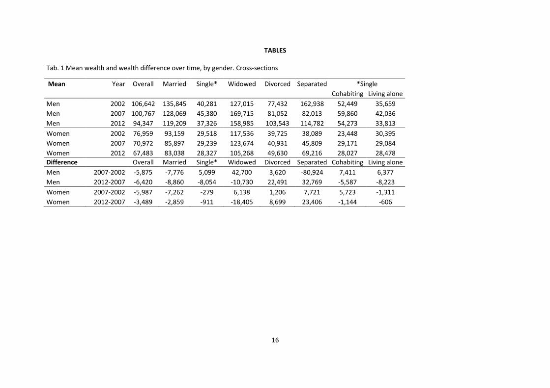
G-SOEP contains information on individual wealth in particular the following assets are details own property (and relative share and relative debt) other real estate (and relative share and relative debt) financial assets (and relative share) business assets tangible assets building loan and private insurance and consumer credits The main dependent variable is net total wealth in 2010 real price In G-SOEP the missing values for wealth are corrected for applying a multiple imputation technique (see Frick et al 2010) for the moment we are only using implicate A but we will later include also the other implicates We apply a 01 top coding and the inverse hyperbolic sine transformation useful to mitigate the effect of the outliners and to deal with skewed variables (with respect to the log transformation the inverse hyperbolic transformation is possible with negative and 0 value) In the first part of the analysis our dependent variables is the difference in net wealth between 2 periods while in the second part is the level in wealth and the gap between men and women The control variables are detailed in Appendix A 5 Descriptives We find that during the period of analysis the real mean wealth levels have been decreasing since 2002 for both women and men (Table 1) The wealth gender gap in 2002 hovered around 30 000 euros at the mean (for a discussion of the sources of the wealth gap in Germany in 2002 see Sierminska et al 2010) it was similar in 2007 and declined to about 27 000 in 2012 The decline in wealth 2002-2007 was similar for women and men (about 6000) and in the subsequent period 2007-2012 it was almost double for men as it was for women (6500 versus 3500) The effect at the median is even more striking A reduction in wealth for men in the pre-crisis period of about 4000 with only a decline of about 400 for women In the subsequent period an increase of 2000 for men and only 500 for women At the median the wealth gender gap increases in 2012 suggesting that there have been different changes for men and women along the wealth distribution Hence the effect of the Great Recession had a differential effect on men compared to women in terms of their wealth level We explore the sources of this differential change
8
We investigate the following possible reasons -different levels of wealth to begin with -risk aversion affecting portfolio composition -more risky portfolio of men than women -more men are self- employed ndash lost businesses -change in labour market attachment of men vs women -more men unemployed then women in post-crisis period In fact our descriptive statistics in Table 5 indicate that women have a lower preference for risk than men (although increasing over time ndash just like men) As shown in Tables 7 and 8 men are more likely to own their home (by about 4 ppt) than women and to have debt either home or consumer debt More generally men are more likely to hold every type of assets (property other real estate financial business tangible building loan and private insurance consumer credits) Interestingly there has been a slight reduction in the percentage of men with business assets and the value of business assets (conditional on owning) is decreasing In addition the percentage of men with building loans and private insurance is decreasing while the same percentage is increasing among women When it comes to married men and women in principle comparable structures could be found although more wealth components are held Women are more likely to have low education but this has decreased by about 6 ppt since 2002 They still have a slight disadvantage in terms of high education but the gap remains at about 4 ppt compared to men This is a striking results since in most other developed countries women are now more educated than men (and this is also true for young German people ndash see OECD 2015) In terms of labour market attachments the number of month in full-time employment for men in the last 5 years has remained about the same with a slight increase for 2007 and subsequent decline while for women the numbers have been steadily increasing although on a slow pace There is still a 1 year difference between the sexes Women are more likely to work part-time but this is declining The number of women not in employment has also been decreasing and is down by 6 ppt since 2002 In terms of the type of employment we can say that the unemployment rate is quite similar for the two groups The share of pensioners has been increasing for men and decreasing for women What is striking is the large 8 ppt increase in white collar employment for women since 2002 which now exceeds that of men by 9 ppt As a result permanent income has been increasing for women and decreasing for men Both groups save regularly at a similar base but the levels for inheritances and gifts received have decreased by 20000 on average compared to the previous period Contrary to previous periods women average levels are now about 20000 more than menrsquos (in 2012) Another aspect that could be affecting this differential changes in wealth levels could be the demographic dimension and more specifically marital status transitions among men and women Marriage is a wealth-enhancing institution because married couples benefit from a joining of assets dual incomes and lowered expenses from economies of scale (Vespa and Painter 2008) See also Vespa and Painter 2011 ldquoOver time marriage positively correlates with wealth accumulation [hellip] We conclude that relationship history may shape long-term wealth accumulation and contrary to existing literature individuals who marry their only cohabiting partners experience a beneficial marital outcomerdquo
9
However in contrast marriage has negative effects on human-capital development for women as they usually suspend their employment career or at least reduce working-hours which impairs individual wealth accumulation for women It is well know that there exists a marriage premium for men in wages and a penalty for women and that substantial income and wealth loses occur due to divorce (Jarvis and Jenkis 1999 Zagorsky 2005) In our sample we find women less likely to be married than men and less likely to be single (by about 5ppt) Women are more likely to be widowed by about 7ppt and slightly more likely to be divorced (2ppt) When it comes to marital changes over the last 5 years we find that there is a 8 ppt gap in 200207 who remained married in favour of men Men are also more likely to remain never married (23-25 versus 18-21) and substantially less likely to remain single after a separation widowhood or divorce (11 versus 22) (even though part of the explanation is that women are overall more likely to be widowed) Thus womenrsquos labour market attachment education and participation in white collar employment could be driving their increase in permanent income and thus affecting the way their wealth has been changing Another aspect could be their changes in marital status which could also affect wealth levels and the composition of the portfolio which changed over the period we are considering 6 Results
61 Changes in wealth the role of explanatory factors
In the next step we isolate in more detail the factors that could affect changes in wealth levels and compare these for women and men We regress the inverse hyperbolic sine differences in wealth in the two periods on multiple explanatory factors In the overall sample (Table 9)4 the determinants of the (inverse hyperbolic sine) difference in the wealth vary over time and across genders Being a migrant has a significant negative effect for both men and women Usually one can argue that this has something to do with disrimination at the labor force however we certainly control for this aspect Thus one may argue that there is a migrant ldquodrawbackrdquo in wealth accumulation An strong factors is whether a person is currently living in East Germany Given the still existing lower earnings level and the general lower wealth level in that fromerly socialist region this still also impairs absolute wealth changes A High educational level (university) is associated with higher asolute wealth changes Besides better labor market changes and thus higher earning profiles for higher educated people this covariate may also point to a better financial literacy which facilitates better investment decisions In addition having a higher educational level is more benefical more women than for men In terms of employment variables we see that full-time employment has a positive effect on changes in wealth which definitely enables individuals to save on a regular basis Having said that long-term
4 In Table A2 we present the results of similar regressions where non-married people are separated into living alone and
cohabiting
10
unemployment has a negative effect on wealth accumulation Income losses due to job losses often offset by dissaving Being self-employed and in a white collar profession has an increasing positive effect only for men
Marital status changes When it comes to marital change it has been found that divorce usually has a negative effect on wealth In our sample this covariate show a negative sign however the effect is not significant The results for our sample indicate that for those that became widows in the past 5 years this increased their wealth as expected B but this effect is stronger for men than for women One potential interpretation is that men usually the one in a partnership who is responsible for investment decissions thus he is more able to handle and invest additional assets Usually one would also a positive effect for those getting married as both partners now profit from joining of assets dual incomes and lowered expenses from economies of scale However no significant effect can be found for our sample One potential explanation for this finding could be that marriage usually coincide with childbirth and finding a new home these additional costs may interfere the wealth accumulation process It can also be that the number of marital status changes in the 5 years is to small to identify significant changes
Portfolio effect The change in wealth will also depend on the performance of the portfolio For example if the portfolio consists of risky assets with a high expected return it will most likely perform better during an expansion compared to a financial crisis While a less risky portfolio with low expected returns would exhibit lower losses as well as lower gains In our results it seems that a preference for risk has a significant effect in the first period People that save have higher gains in wealth with a stronger effect for women In the following we examined whether people were purchasing or selling property and whether they were getting themselves into consumer debt in other to smooth consumption or finance their consumption needs The overall conclusion seems to be that people with property or those that purchased property are better off than In terms of debt those that get rid of consumer credits or property debts show a positive wealth change as they are forced to pay back their loan on a regular basis However those who newly borrowed have a negative effect on wealth change A very strong negative effect can also observed for those how changed their tenure status from owner occupiers to tenants Although in case of a sale one would assume that net worth Would not change while there is a shift from property wealth to financial assets in many cases bestowals to children or other relatives may the causal explanation
Quintile
People at every other quintile of net wealth lose with respect to people in the first quantile Those in the group of having debts in t0 are forced to pay back their loans on a regular basis and thus show positive wealth changes Those who had zero wealth in t0 are often young people who are at the beginning of the typical life cycle process of saving Thus with increased earnings the possibility to save also increase for this group On the other side those at the top are often elderly who hand over their wealth (by bestowals) to the next generation Additionally the higher the wealth the higher is also the probability to loose in absolute amounts
11
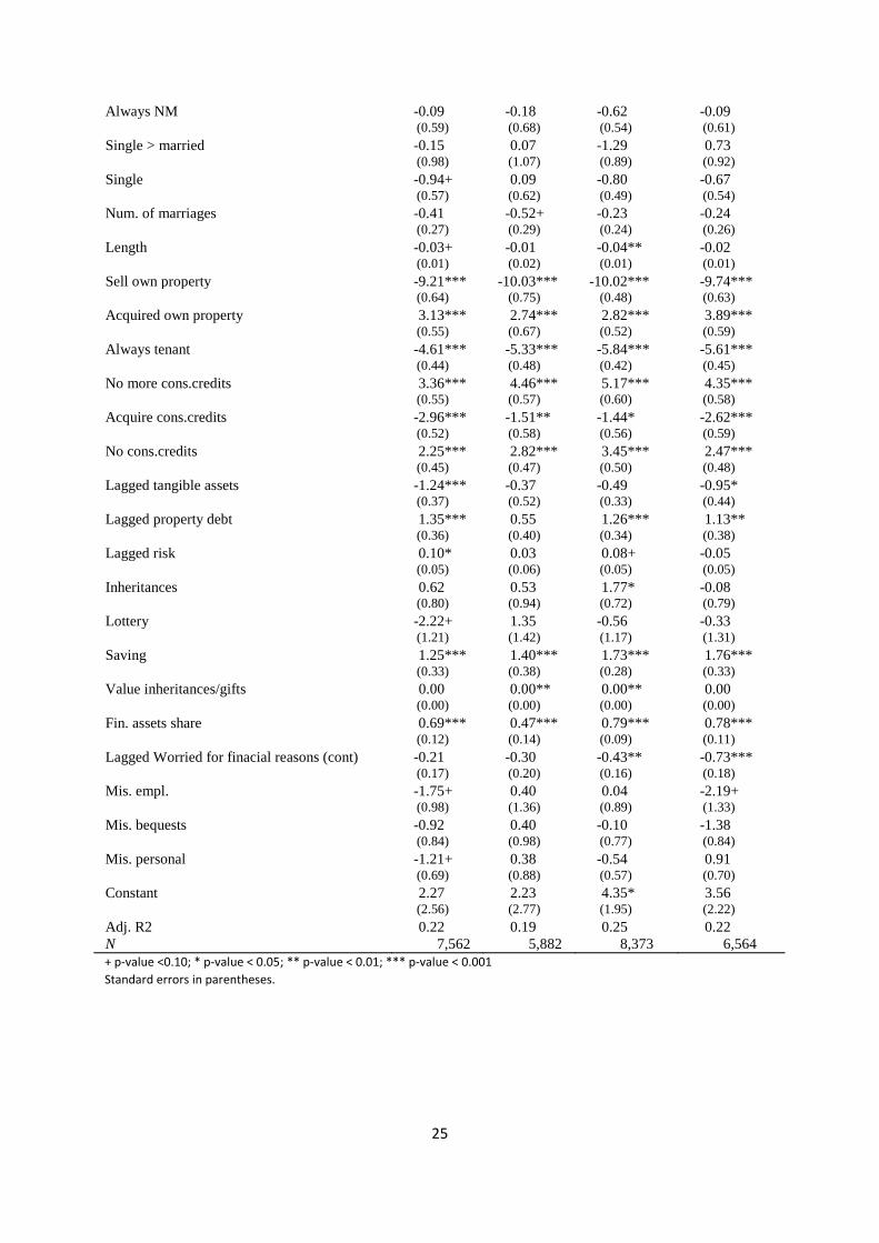
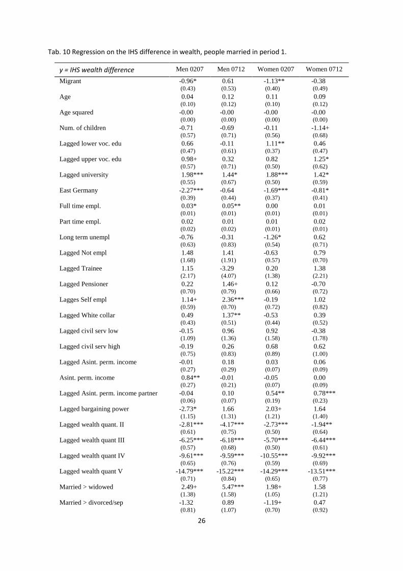
Married only When we perform the regression only on those that were married we observe some changes (Table 10) We also include additional variables such as the lagged income of the partner and lagged bargaining power First of all the labour market and employement variables lose significance for women that are married and the partner income is positive and statistically significant for women Being a migrant only matters in the first period With respect to the changes in marital status widowhood has a larger positive impact for men more than women Divorce has a negative impact in the first period significant only among women The number of marriages has a negative effect on changes in wealth but only in the second period for both genders The risk variable is no longer significant for women Saving still has a positive effect on both groups
62 Comparing the gender wealth gap in different periods
621 Regressions As a second step we investigate the gender wealth gap between married men and women in 2007 and 2012 In this case our dependent variable is the IHS of wealth (not the difference) To perform the OB decomposition we first of all run separated regressions for men and women in 2007 and in 2012 The effect of the control variables is similar to the previous specification but some changes can be noticed Being a migrant has a negative effect on the wealth of women also in the second period If we look back to the descriptive it can be noticed that there is an increase of 1st generation migrants among women while the percentage is stable among men Both the descriptive and the regressions point toward a different migration patter of migrant men and women to Germany Age has a positive effect larger in 2012 The level of education has a larger and effect for women than for men in 2007 while in 2012 the positive effect of education is similar for men and women Full time and part-time employment has a stronger effect in 2007 than in 2012 for both men and women On the other hand the long term unemployment has a stronger negative effect in 2012 for men wile for women it is similar in the two periods With respect to the occupations being self-employed has a positive and significant effect on wealth for men only larger in the first period the regression is reflecting what we have already seen in the descriptive that the value of business assets was decreasing over time Becoming widowed has no significant impact on the level of wealth while having a divorce in the previous 5 years has a negative impact on men wealth stable over time For women the effect of a divorce is negative and significant only in the first period On the other hand the negative effect of the number of marriages is stronger in 2012 Savings have a larger positive effect for women
622 OB decomposition
12
The OB decomposition is presented in Table 12 The gender wealth gap at the mean decreases from 2007 to 2012 Moreover the explained gender wealth gap is smaller and the unexplained component which is negative is larger In other words the wealth gap decreases as a consequence of smaller differences in characteristics between men and women but also due to slightly better returns for women which partially compensate The level of education which had no significant effect on the explained component in 2007 in 2012 has a positive effect on the explained gap indeed the returns to education in 2012 are very similar but men are more likely to have higher education than women On the other hand the occupational status is no longer significant in explaining the level of wealth and thus does not explain wealth differences among the two groups Permanent income has a smaller effect in 2012 while the income of the partner contributes more in reducing the explained gap It is worth noting that changes in property debt and in consumer credits have both a smaller (absolute) effect on the gap Both property and consumer credits no longer have a significant effect on the unexplained component in 2012 The largest effects come from permanent income and from the partner income the permanent income has a large and significant effect on the unexplained gap while the permanent income of the partner has a significant effect which contributes to reducing the unexplained gap The coefficients on these work in the opposite direction and even though they are still very large they are smaller in absolute terms in 2012 In addition the level of education (which had a negative effect on the unexplained gap) and the labour market status (positive) are not significant anymore indeed full time and part-time unemployment have no significant impact on the level of wealth in 2012 while the higher return to education for women which were present in 2007 are now at the same level for both sex Overall it seems that the smaller return to permanent income of women largely affect the gap as can be seen from the regressions as well the permanent income has a positive effect for men but almost no effect for women compensated by the higher effect for women wealth of partner income (Still ndash men do not compensate enough since the gwg among married is larger than in the total population)
623 FIRPO decomposition The results from the detailed decomposition serve to complement the above OB decomposition at the mean We examine these at the 10th 50th and 90th percentile in Table 13 As in the mean decomposition the wealth gap has decreased from 2007 and 2012 but the largest change is observed at the median There has not been much change at the top of the distribution either for women nor for men The role of education in explaining the gap is more or less constant throughout the distribution Though labour market status differences did not significantly explain the wealth gap at the mean they do explain a sizeable portion of the gap at the median and the upper half of the distribution In fact the differences have a diminishing effect on the gap as the share of men working full-time changed and the share of women working full-time and part-time increased in the first period (from 2002 to 2007) (Table 6) Subsequently the number decreases a bit from 2007 to 2012 and the effect is no longer significant in the second period
13
Differences in occupational status consistently contribute to the gender wealth gap over time As in our previous work differences in permanent income play a sizeable role ndash although in the second period this declines at the median Permanent income of the partner is not significant in explaining the gender wealth gap throughout the distribution Another factor that plays a sizeable role in the first period but then diminishes in size is the status of property ownership It explains about one-half and almost all the gap in the second period at the median Risk is only significant in the second period for the top half of the distribution In terms of returns Differences in labour market returns are sizeable and contribute to the gap only in the first period Overall returns in permanent household income have a diminishing effect on the gap in the first period and an effect twice as large in the second period Seems as if womenrsquos income works to diminish the gap The differences in the return to the share of financial assets in the portfolio also seem to diminish the gap 7 Summary and conclusions To be completed
14
References Blau FD and Kahn LM (1997) Swimming Upstream Trends in the Gender Wage Differential in the
1980s Journal of Labor Economics 15 1-42
Blau FD and Kahn LM (2000) Gender Differences in Pay Journal of Economic Perspectives 14 75-99
Blinder AS (1973) Wage discrimination reduced form and structural estimates Journal of Human Resources 8(4) 436-455
Brenke K (2015) Wachsende Bedeutung der Frauen auf dem Arbeitsmarkt DIW Wochenbericht Nr 5-2015 S 75-86
Cartwright Edward (2011) Behavioral econimcs Routledge New York Deere CD and Doss CR (2006) The gender asset gap What do we know and why does it matter
Feminist Economics 12(1-2) 1-50 EUROSTAT (2014) Wachstumsrate des realen BIPmdashVolumen (httpeppeurostateceuropaeutgm tabledotab=tableampinit=1ampplugin=1amplanguage=deamppcode=tec00115) Accessed 29 Oct 2014 Eurostat (2015) Life expectancy at birth by sex
Firpo S Fortin N M and Lemieux T (2009) Unconditional Quantile Regressions Econometrica 77(3) 953-973 Frick JR Grabka MM and Marcus J (2010) Editing und multiple Imputation der Vermoumlgensinformation 2002 und 2007 im SOEP DIW Data Documentation No 51 Berlin Grabka M Marcus J and Sierminska E (2013) Wealth distribution within couples Review of
Economics of the Household online first 101007s11150-013-9229-2 Jarvis S and Jenkis SP (1999) Marital splits and income changes Evidence from the British
Household Panel Survey Population Studies 3(2) 237-254) Lusardi A amp Mitchell O S (2008) Planning and financial literacy How do women fare American
Oaxaca R L (1973) Male-Female Wage Differentials in Urban Labor Markets International Economic Review 14(3) 693-709
OECD (2012) Closing the Gender Gap Act Now OECD Publishing httpdxdoiorg1017879789264179370-en
OECD (2015) Education and employment What are the gender differences Education Indicator in Focus n 30 Paris OECD
Sierminska E Frick JR and Grabka M (2010) Examining the gender wealth gap Oxford Economic Papers 62(4) 669-690
UNECE (2014) Statistical Database Fertility families and households httpw3uneceorgpxwebdatabaseSTAT30-GE02-Families_householdslang=1
US Census Bureau (2014) Americarsquos Families and Living Arrangements 2014 Family groups httpwwwcensusgovhhesfamiliesdatacps2014FGhtml
Vespa J and Painter MA (2008) ldquoThe Paths to Marriage Cohabitation and Marital Wealth Accumulationrdquo Paper presented at the Population Association of America Meeting New Orleans Vespa J Painter MA (2011) Cohabitation history marriage and wealth accumulation Demography 48(3)983-1004 doi 101007s13524-011-0043-2 Warren T Rowlingson K and Whyley C (2001) Female finances Gender Wage Gaps and Gender
Assets Gaps Work Employment and Society 15 465-488
Westermeier C and Grabka MM (2015) Significant Statistical Uncertainty over Share of High Net Worth Households Economic bulletin no 14+15 p 210-219
Zagorsky JL (2005) Marriage and divorce impact on wealth Journal of Sociology 41(4) 406ndash424
15
FIGURES
Fig 1 Wealth density over time (truncated)
16
TABLES Tab 1 Mean wealth and wealth difference over time by gender Cross-sections
Mean Year Overall Married Single Widowed Divorced Separated Single
Cohabiting Living alone
Men 2002 106642 135845 40281 127015 77432 162938 52449 35659
Men 2007 100767 128069 45380 169715 81052 82013 59860 42036
Men 2012 94347 119209 37326 158985 103543 114782 54273 33813
Women 2002 76959 93159 29518 117536 39725 38089 23448 30395
Women 2007 70972 85897 29239 123674 40931 45809 29171 29084
Women 2012 67483 83038 28327 105268 49630 69216 28027 28478
Difference
Overall Married Single Widowed Divorced Separated Cohabiting Living alone
Men 2007-2002 -5875 -7776 5099 42700 3620 -80924 7411 6377
Men 2012-2007 -6420 -8860 -8054 -10730 22491 32769 -5587 -8223
Women 2007-2002 -5987 -7262 -279 6138 1206 7721 5723 -1311
Women 2012-2007 -3489 -2859 -911 -18405 8699 23406 -1144 -606
17
Tab 2 Mean wealth and wealth difference over time by gender Panel
+ p-value lt010 p-value lt 005 p-value lt 001 p-value lt 0001 Standard errors in parentheses
33
APPENDIX
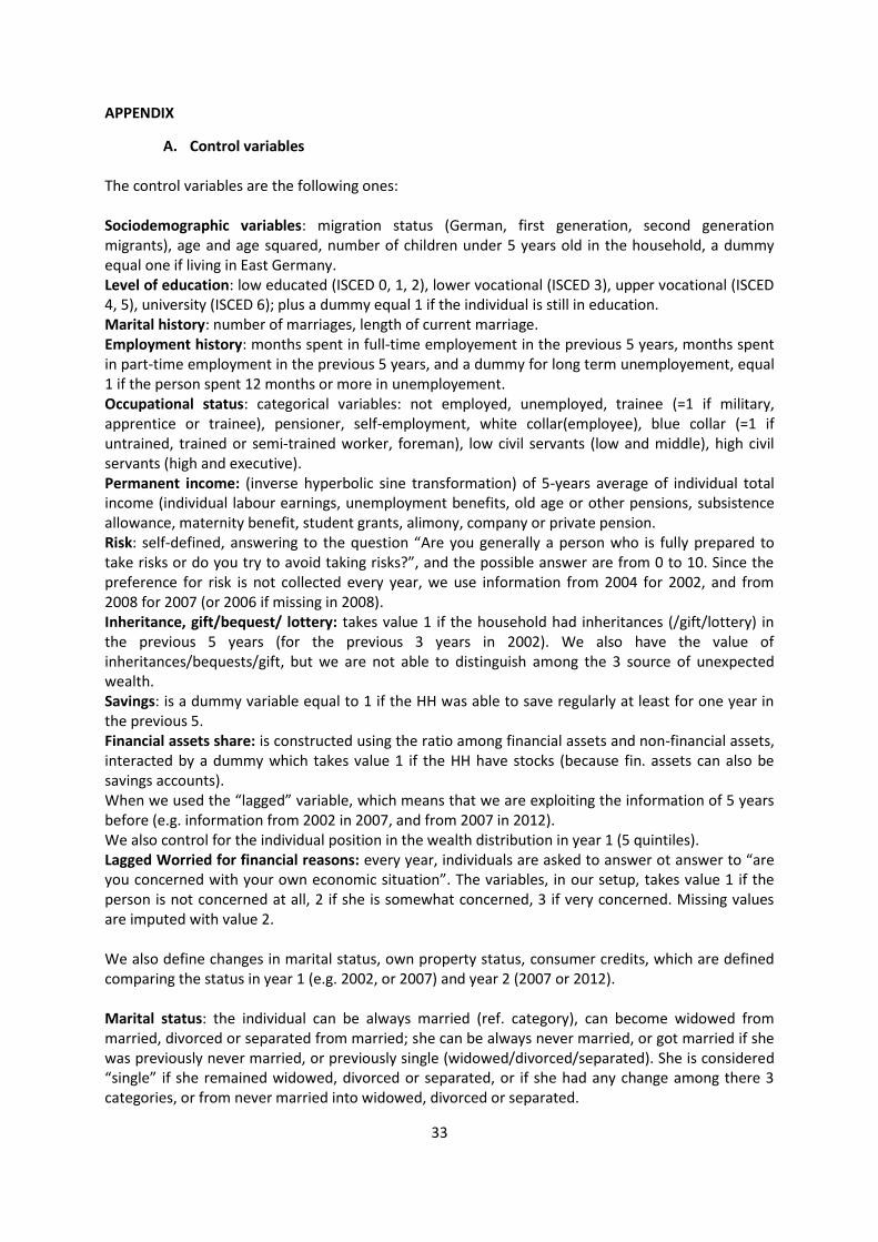
A Control variables The control variables are the following ones Sociodemographic variables migration status (German first generation second generation migrants) age and age squared number of children under 5 years old in the household a dummy equal one if living in East Germany Level of education low educated (ISCED 0 1 2) lower vocational (ISCED 3) upper vocational (ISCED 4 5) university (ISCED 6) plus a dummy equal 1 if the individual is still in education Marital history number of marriages length of current marriage Employment history months spent in full-time employement in the previous 5 years months spent in part-time employment in the previous 5 years and a dummy for long term unemployement equal 1 if the person spent 12 months or more in unemployement Occupational status categorical variables not employed unemployed trainee (=1 if military apprentice or trainee) pensioner self-employment white collar(employee) blue collar (=1 if untrained trained or semi-trained worker foreman) low civil servants (low and middle) high civil servants (high and executive) Permanent income (inverse hyperbolic sine transformation) of 5-years average of individual total income (individual labour earnings unemployment benefits old age or other pensions subsistence allowance maternity benefit student grants alimony company or private pension Risk self-defined answering to the question ldquoAre you generally a person who is fully prepared to take risks or do you try to avoid taking risksrdquo and the possible answer are from 0 to 10 Since the preference for risk is not collected every year we use information from 2004 for 2002 and from 2008 for 2007 (or 2006 if missing in 2008) Inheritance giftbequest lottery takes value 1 if the household had inheritances (giftlottery) in the previous 5 years (for the previous 3 years in 2002) We also have the value of inheritancesbequestsgift but we are not able to distinguish among the 3 source of unexpected wealth Savings is a dummy variable equal to 1 if the HH was able to save regularly at least for one year in the previous 5 Financial assets share is constructed using the ratio among financial assets and non-financial assets interacted by a dummy which takes value 1 if the HH have stocks (because fin assets can also be savings accounts) When we used the ldquolaggedrdquo variable which means that we are exploiting the information of 5 years before (eg information from 2002 in 2007 and from 2007 in 2012) We also control for the individual position in the wealth distribution in year 1 (5 quintiles) Lagged Worried for financial reasons every year individuals are asked to answer ot answer to ldquoare you concerned with your own economic situationrdquo The variables in our setup takes value 1 if the person is not concerned at all 2 if she is somewhat concerned 3 if very concerned Missing values are imputed with value 2 We also define changes in marital status own property status consumer credits which are defined comparing the status in year 1 (eg 2002 or 2007) and year 2 (2007 or 2012) Marital status the individual can be always married (ref category) can become widowed from married divorced or separated from married she can be always never married or got married if she was previously never married or previously single (widoweddivorcedseparated) She is considered ldquosinglerdquo if she remained widowed divorced or separated or if she had any change among there 3 categories or from never married into widowed divorced or separated
34
Property the individual can be always owner (ref category) sell the property acquire property or be always tenant Consumer credits the individual can have consumer credits in both periods (ref category) get rid of them take out consumer credits or never have consumer credits In addition we also include some ldquomissing variablesrdquo ldquomissing employmentrdquo takes value 1 if the employment history or the occupational category was missing ldquomissing bequestrdquo takes value 1 if the inheritance gifts lottery (or their value) saving variable is missing ldquomissing personalrdquo takes 1 if variables for education marital status or marital history migration background risk preference are missing In the regression for married couples we also include the permanent income of the spouse and a variable controlling for the bargaining power this variable is constructed as the ratio among the personal permanent income and the permanent income of the couple (partner permanent income added to the personal one) When we perform the Oaxaca-Blinder decomposition and the Firpo decomposition the explanatory variables are grouped in the following way Groupmig migratory status Groupage age and ande squared Groupkids number of kids Groupeduc lagged level of education or lagged still in education Grouploc residence in East Germany Grouplm labour market (full time parttime unemployment not employed) Groupoccup lagged occupational status (trainee pensioner self empl white collar civil servants low or high) Groupinc personal permanent and lagged permanent income Grouppinc partner lagged income Groupbarg bargaining power Groupmarstat changes in marital status Groupmarr number of marriages and length Groupprop changes in own property Groupcdebt changes in consumer credits Grouport lagged real estate lagged tangible assets Grouprisk lagged risk Groupsav inheritances lottery savings Groupvalsav value of inheritances Groupfinshare financial assets share Groupworried Lagged Worried for financial reasons Groupother missing variables
35
B Additional tables
Tab B1 Sample size
Cross-sections Year Overall Married Single Widowed Divorced Separated Single
2 To conduct the analysis we focus on the changes for 2002-2007 and 2007-2012 To do so we need to keep the same individuals over the 2 periods We avoid doing so for the 3
periods (keeping the same individuals from 2002 to 2012) because the attrition would cause the loss of too many observations The mean and median wealth gap are presented both
considering the 3 samples for the 2002 2007 2012 cross-sections (ldquoCross-sectionsrdquo) and the 2 samples one for 2002-2007 and the other one for 2007-2012 (ldquoPanelrdquo)
36
Tab B2 Regression on the IHS difference in wealth overall sample (controlling for cohabiting people)
y = IHS wealth difference Men 0207 Men 0712 Women 0207 Women 0712
Migrant I -089 049 -087 -093
(038) (049) (034) (043)
Migrant II -114 008 -090+ 017
(055) (060) (050) (055)
Age 002 -000 006 012+
(007) (007) (006) (007)
Age squared 000 000 -000 -000
(000) (000) (000) (000)
Num of children -070+ -074 -044 -068
(041) (050) (036) (044)
Lagged lower voc edu 018 041 089 031
(035) (044) (027) (033)
Lagged upper voc edu 079+ 123 059 113
(044) (053) (037) (045)
Lagged university 166 223 198 183
(043) (050) (037) (042)
Lagged in educ 007 170 240 239
(116) (136) (090) (107)
East Germany -194 -076 -162 -125
(028) (031) (025) (028)
Full time empl 003 005 002 002
(001) (001) (001) (001)
Part time empl 002 002 002 002
(002) (002) (001) (001)
Long term unempl -113 -023 -132 034
(044) (057) (039) (047)
Lagged Not empl 106 046 -021 112
(111) (126) (045) (053)
Lagged Trainee -002 106 057 210
(066) (082) (060) (074)
Lagged Pensioner 035 153 -003 -011
(057) (063) (051) (056)
Lagges Self empl 120 226 -018 153
(047) (054) (057) (063)
Lagged White collar 081 124 -033 083
(033) (039) (033) (039)
Lagged civil serv low 000 070 069 215+
(084) (103) (115) (126)
Lagged civil serv high -032 007 053 132+
(061) (068) (068) (077)
Lagged IHS perm income -012 010 007 008
(010) (011) (005) (006)
IHS perm income 052 006 -002 001
(015) (012) (006) (007)
Lagged wealth quant II -253 -308 -234 -247
(039) (047) (032) (040)
Lagged wealth quant III -622 -633 -613 -673
(039) (047) (034) (040)
Lagged wealth quant IV -925 -944 -1036 -965
(048) (054) (044) (048)
Lagged wealth quant V -1431 -1445 -1407 -1338
(053) (060) (049) (055)
Married gt divorcedsep -108 012 -121+ 078
(074) (091) (064) (084)
Married gt widowed 260 454 157 312
(119) (133) (078) (087)
Cohabit gt married 112 114 -026 027
37
(082) (090) (074) (082)
Always cohabit 033 -022 -028 061
(087) (096) (078) (087)
Cohabit gt singleNM -108 047 015 -121
(131) (151) (112) (138)
NM gt married -053 -051 -065 240
(090) (120) (083) (107)
NM gt cohabit 009 101 116 065
(091) (105) (081) (095)
Always NM 001 -078 -091 -083
(066) (076) (061) (069)
Single gt married 004 031 -277 165+
(097) (104) (092) (098)
Single -099+ 010 -103 -083
(057) (063) (049) (054)
Num of marriages -036 -063 -013 -038
(029) (031) (025) (027)
Length -003+ -002 -004 -002+
(001) (002) (001) (001)
Sell own property -925 -1001 -1006 -980
(064) (075) (048) (063)
Acquired own property 310 278 286 392
(055) (067) (052) (059)
Always tenant -463 -527 -585 -555
(044) (048) (042) (045)
No more conscredits 339 445 514 436
(055) (057) (060) (058)
Acquire conscredits -292 -147 -147 -260
(052) (058) (056) (059)
No conscredits 231 288 348 258
(045) (047) (050) (048)
Lagged tangible assets -124 -039 -043 -087
(037) (052) (033) (044)
Lagged property debt 133 052 126 108
(036) (040) (034) (038)
Lagged risk 011 003 008+ -004
(005) (006) (005) (005)
Inheritance 088 060 147 099
(073) (087) (068) (073)
Gift 135+ 030 058 031
(072) (085) (066) (074)
Lottery -189 129 -093 025
(118) (138) (115) (129)
Saving 130 147 183 188
(033) (038) (028) (033)
Value inheritancesgifts 000 000 000 000
(000) (000) (000) (000)
Fin assets share 070 047 078 076
(012) (014) (009) (011)
Mis empl -178+ 039 005 -220+
(098) (136) (089) (133)
Mis bequests -038 032 -069 -066
(076) (089) (070) (077)
Mis personal -147+ 019 -075 092
(075) (094) (065) (077)
Constant 120 192 353+ 133
(253) (271) (190) (218)
R2 022 019 025 022
N 7562 5883 8373 6564
+ p-value lt010 p-value lt 005 p-value lt 001 p-value lt 0001 Standard errors in parentheses
38
Tab B3 Regression on the (asint) wealth levels people never married in period 1 Y=as Wealth
Men 07 Men 12 Women 07 Women 12
Migrant -127 -045+ -049 -059
(037) (023) (036) (043)
Age -003 021 009 015
(010) (005) (007) (009)
Age squared 000 -000 -000 -000
(000) (000) (000) (000)
Num of children -050 -005 -072 -043
(040) (031) (030) (038)
Lagged lower voc edu 017 042 039 026
(039) (027) (037) (046)
Lagged upper voc edu 063 085 034 038
(057) (031) (048) (058)
Lagged university 129 102 136 167
(058) (029) (051) (059)
Lagged in educ 017 158 258
(081) (067) (085)
East Germany -020 -037 -039 -102
(031) (018) (029) (033)
Full time empl 004 001 002 002
(001) (001) (001) (001)
Part time empl 001 -000 003 002
(002) (001) (001) (001)
Long term unempl -143 -107 -147 -040
(043) (036) (043) (054)
Lagged Not empl -094 114 -053 178
(109) (084) (065) (078)
Lagged Trainee -041 -337 114 214
(048) (168) (047) (058)
Lagged Pensioner 052 -006 165 -010
(120) (034) (102) (136)
Lagges Self empl 097 111 276 144
(064) (030) (082) (091)
Lagged White collar 049 019 119 149
(040) (022) (041) (050)
Lagged civil serv low 120 096 -039 195
(107) (059) (131) (143)
Lagged civil serv high 001 001 -011 015
(110) (037) (083) (103)
Lagged Asint perm income 004 019+ -001 001
(007) (010) (006) (007)
Asint perm income 031 016+ 043 026
(011) (009) (012) (012)
NM gt married 232 137 166
(170) (172) (159)
Single 206 127 149
(207) (219) (189)
Num of marriages -257+ -073 -159 -044
(148) (018) (155) (137)
Length 015 -001 016 -016
(019) (001) (017) (021)
Sell own property -227+ -574 -375 -263+
(130) (041) (111) (144)
Acquired own property -198 -001 -029 -076
(079) (036) (080) (091)
Always tenant -482 -516 -471 -459
(068) (020) (070) (076)
No more conscredits 757 455 1034 687
39
(078) (032) (084) (077)
Acquire conscredits 136 142 335 026
(066) (033) (070) (071)
No conscredits 817 486 1071 738
(061) (025) (064) (062)
Lagged tangible assets 057 101 044 021
(055) (029) (055) (065)
Lagged property debt -006 023 103 -064
(085) (020) (086) (094)
Lagged risk -003 -001 010+ -005
(006) (003) (006) (007)
Inheritance 217 073 134 063
(076) (061) (065) (068)
Lottery -145 033 252 127
(121) (081) (126) (151)
Saving 208 238 216 203
(037) (023) (034) (040)
Value inheritancesgifts 000 000+ 000 000
(000) (000) (000) (000)
Fin assets share 071 067 052 062
(011) (009) (008) (009)
Lagged Worried for finacial reasons 004 -037 -035+ -043+
(020) (012) (019) (022)
Mis empl -036 -071 -342 -324
(204) (073) (216) (227)
Mis bequests 069 055 130+ -031
(085) (063) (074) (076)
Mis personal -098 -002 -077 -020
(060) (063) (060) (070)
Constant -304 -592 -1021 -549
(273) (204) (228) (264)
Adj R2 041 046 048 043
Obs 1781 3831 1667 1315
+ p-value lt010 p-value lt 005 p-value lt 001 p-value lt 0001 Standard errors in parentheses
40
Tab B4 Oaxaca Blinder decomposition (2007 and 2012) never married in period 1 Y=as Wealth
1 Introduction Given the growing reliance of economic well-being on private assets including old age provision in the form of pensions and retirement income there is a growing interest in the study of private wealth However until recently the information about private wealth were scarce or not existent in many European countries With the Household Finance and Consumption Survey (HFCS) this gap is signicficantly shortened But still there arises the problem that private wealth is typically only surveyed at the household level by a reference person - as has been done in the HFCS or even also in the SCF - which does not allow for any intra-household analyses of private wealth Though past literature has stressed the importance of looking at intra-household inequalities (Deere and Doss 2006) and it has shown to lead to substantial differences in wealth levels among women and men (Sierminska et al 2010 Grabka et al 2013) Moreover Germany is also an interesting subject for wealth analyses as it was one of the OECD countries which had been hit hardest by the financial crisis ndash the so-called Great Recession in 20082009 GDP dropped by more than 5 in 2009 which was the strongest recession in Germany after World War II Other West European countries were not affected as much by the Great Recession1 It can be assumed that a financial crisis usually should have an impact on financial assets and net worth of private households However given that women are believed to be less risk prone (Cartwright 2011) thus reducing their expected return on a portfolio ndash at the same time higher risk aversion may shelter from unexpected asset fluctuations that had place during the Great Recession Thus we also intend to test whether this lower risk aversion allowed women to lose less (or maybe allowed to gain) during the Great Recession in Germany compared to men With three observations years of the German Socio-Economic Panel we are able to describe the gender specific wealth accumulation before the crisis (2002-2007) and during the crisis (2007-2012) It can be assumed that absolute wealth changes might be more prevalent for men given the higher wealth levels of men preceding the crisis their higher risk behavior in financial investments and income losses as the manufacturing and engineering industry in Germany ndash which by the majority employ men ndash shrank by almost 20 during the Great Recession in Germany and heavily made use of short-term compensation2 With unique micro-data about private wealth at hand we are able to analyze the gender difference in wealth levels and wealth accumulation in Germany given that the German Socio-Economic Panel (SOEP) is one of the very rare data-sources which collects wealth information at the individual level Besides this methodological precondition Germany also provides an interesting context for the analyses of the gender wealth gap womenrsquos attachment to the labor market has been significantly growing While the female labour force participation rate was only 53 in 1993 this share has been markedly increased by 10 percentage points to almost 63 in 2013 (Brenke 2015) and is now clearly above the Euopean level With entry into employment this allows women to earn their own money and to accumulate wealth Thus we like to answer the question how this changed labor market participation had any affects on the wealth distribution of women and men Given that women on average live a few years longer than man (Eurostat 2015) in combination with lower entitlements from public pension systems (the gender pension gap for mandatory pensions is
1 The Great Recession in Germany last for 12 months between Q2-2008 until Q1-2009 measured by quarter-on-quarter changes of seasonally adjusted real GDP For example in 2009 GDP in Spain contracted by only 38 in France by 32 and even in Portugal only by 29 (Eurostat 2014) 2 The basic idea of short-time compensation is that a firm with financial difficulties can apply for financial aid from the Federal Employment Agency to prevent the need for layoffs In return the firm has to reduce working hours and pay The replacement rate is 60 for single workers and 67 for workers with dependents
3
about 34 in OECD countries ndash OECD 2012) there is pressure for women to take care of their own private wealth This is reinforced by the growing number of single-headed female households (UNECE 2014 US Census Bureau 2014) and in particular elderly females which suffer more from old-age poverty than men (OECD 2012) In this paper we set out to investigate the explanatory factors of that have contributed to changing wealth levels covering the period of the Great Recession Given the large labor market changes which have taken place during this time in Germany we expect the process of accumulating wealth to have changed Women have increased their labor market participation while men have had it more difficult We compare the role of factors for women and men Consequently in the second part of the paper we extend the existing literature and discuss the changing gender wealth gap which has resulted from this changes both at the mean and across the wealth distribution The rest of the paper is organised as follows The following section outlines the literature and conceptual backgrounds Section 3 describes the methods Section 4 presents the data The descriptives and empirical results are in Section 5 and 6 respectively followed by a summary and conclusions in Section 7 2 Literature and Conceptual Background As commonly known wealth is accumulated according to the standard life-cycle model where the stock of assets in the current period is the outcome of past decisions regarding investment labor market outcomes savings and consumption As discussed in Sierminska et al (2010) differences in any of these factors will give rise to a different accumulation pattern and consequently a different portfolio structure Consequently any type of macro-economic or life-shock will have a differential impact on individual portfolios according to this structure Among possible causes that have been shown to affect wealth accumulation differently for women and men are women and men save differently women have a weaker attachment to the labor market and women and men invest differently with diverging levels of returns The literature indicates that women and men differ in the risk attitudes with women being less risk tolerant and more risk-averse (Cartwright 2011) which would lead to less risky portfolios and lower rates of return Addionally financial literacy (eg Lusardi and Mitchell 2008) influence investment decisions It is shown that men and women differ in their financial knowledge which also leads to more conservative investments done by women Apart from having differential returns a more risk-loving individual having invested in risky assets will be more exposed to fluctuations in the (stock) market Similarly a person whose majority of assets are invested in real estate property will be very susceptible to changing house prices One of the the more important factors that has been shown in Sierminska et al (2010) to explain male-female differences in wealth accumulation is labor market differences It is not only the lower labor market participation rate of women the lower working hours as women commonly work part-time compared to men with the standard pattern of a continuous full-time employment but even also the still existing gender pay gap which impairs the wealth accumulation for women (Warren et al 2001) Even when holding savings rates constant women are thus expected to accumulate lower levels of wealth (eg Blau and Kahn 1997 2000)
4
Other factors which may affect wealth accumulation and in particular its differences by gender are for example inheritance and bestowals if women are men have differential access to these One factor important for this paper would also be occupations Women and men ten to cluster in different occupation that have different perspectives in advancement as well as different exposures to labor market flucturations and thus could be differentially exposed to the consequences of the Great Recession During the last financial crisis in Germany the labor market has been differentially affected across occupations Over the last two decades the labor market in Germany has observed some major changes Not only women have substanitally increased their participation rates but numerous labor market reforms have been implemented (Hartz reforms) (Dustmann et al 2014 Brenke 2015) which as we will show could have had an impact on the wealth accumulation of women and men Based on the overview of the literature several hypothesis come to mind that could be tested within our framework Hypothesis 1 A more risk-loving individual (men) having invested in risky assets will be more exposed to fluctuation in the stock market Similarly a person whose majority of assets are invested in real estate property will be very susceptible to changing house prices (men) and this will result in the changing wealth levels Hypothesis 2 Womenrsquos increased attachment to the labor market will improve their position in the wealth distribution Hypothesis 3 Higher prevelance of part-time work will have a negative (decreasing ) effect on wealth Hypothesis 4 The changing impact of labor market attachment will have a stronger impact on womenrsquos wealth Hypothesis 5 Labor market factors are less important for older individuals We will consequently address these in our results section 3 Methods As discussed in the introduction we will first focus on what were the causes of the changes in wealth over this period and then we will investigate the changing wealth gap
31 Change in wealth
To analyse the changes of wealth over time we starting by estimating a wealth equation by OLS considering the change in variables instead of the level ones The equation is
(1)
Where is the change in the level of (inverse hyperbolic real) net wealth ie
is a vector of control variables observed in the second period (ie in 2007 for the comparison
2002-2007 and in 2012 for the comparison 2007-2012) migratory background age age squared living in West or East Germany number of children below age 5 in the household number of
5
marriages length of current marriage number of months spent in fulltime and in parttime work in the previous 5 years long term unemployement in the previous 5 years (inverse hyperbolic real) permanent income household inheritances bequestgifts lottery winning and their value over the previous 5 years household savings in the previous 5 years and share of financial assets
is a vector of control variables observed in the first period (ie in 2002 for the comparison 2002-
2007 and in 2007 for the comparison 2007-2012) level of education (controlling also if shehe was still in education) occupational status (inverse hyperbolic real) permanent income tangible assets own property debts and position in the wealth distribution
is a vector of changes in control variables between and change in marital status change
in own property assets change in consumer credits is a random error normally distributed
are the parameters to be estimated by OLS
Equation 1 is estimated separately for men and women and for the period 2002-2007 2007-2012 In addition we also estimate the same equation for married individuals In that case we also control
for the permanent income of the spouse in and for the bargaining power in
32 Gender wealth gap in different periods
The second contribution of our paper is to examine the evolution of the gender wealth gap over time particularly before and after the crisis In the first instance we only consider those individuals that were married in period 13 We focus on married people to see clearly the changing role of explanatory factors for a more homogenous group which nevertheless comprises about 50 of the population and because we have the unique opportunity of doing so with our individual level data In this case we first apply the Oaxaca-Blinder decomposition (Blinder 1973 Oaxaca 1973) at the mean and then Firpo Fortin Lemieux decomposition (Firpo et al 2009) for the whole distribution The Oaxaca-Blinder decomposition relies on the estimation of the following equation for men and women similar to equation 1 but where the dependent variables is the (inverse hyperbolic real) net worth and not its change over time
(2)
The OB decomposition is the standard one (3)
Where =male =female The first component captures the effect which can be attributed to differences in characteristics while the second one captures the effect of differences in returns
33 Detailed decomposition of the gender wealth gaps
3 Throuout the paper with ldquoperiod 1rdquo we indicate 2002 in the comparison 2002-2007 and 2007 in the
comparison 2007-2012
6
In the final section of the paper we focus in performing a detailed decomposition of the gender wealth gaps over time This technique introduced in Firpo et al (2009) allows to decompose differences between two distributions of a variable It allows to have the individual contribution of each explanatory variable considered in the analysis via the characteristics and returns components In our case it will allow us to identify the explanatory factors and how the differences in their distribution and returns change due to the financial crisis and the changing labor market circumstances (characteristics and returns) in order to understand what is contributing to the gender wealth gap in Germany
The Firpo Fortin Lemiuex method is regression based which allows to apply it in a simiar way as the OB method The technique relies on the estimation of a regression where the dependent variable is replaced by a recentered influence function (RIF) transformation and so any distributional statics can be decomposed based on the regression results
In our case we will focus on the differences in quantiles
)()(
^^__^____
QF
QM
M
QM
FM
Q XXX (4)
Where Q is the difference in quantile (or other statistic) τ of the wealth distribution
FM
XX____
are the average observed characteristics for men (M) and women (F) FM
Q
^
are the
coefficients obtained from the regression of the RIF variables of quantile Qτ on the set of explanatory variables for women (F) and men (M) The first terms in equation (4) captures the effect on the differential between the distributions caused by differences in characteristics (explained component) The second term corresponds to the effect of the coefficient in which the contribution of each individual explanatory factor can be distinguished 4 Data We use the German Socio-Economic Panel (G-SOEP) a representative longitudinal survey on individuals in private household The survey started in 1984 in West Germany and extended to states in East Germany before the reunification in 1990 Every year about 15000 household are interviewd (25000 people) In 2002 there was a boost of higher-income people to better capture the upper margin of the income and wealth distribution There were other refreshment samples in 2006 2009 and 2011 while we couldnrsquot include the refreshment of 2012 since they were not asked information on wealth Although the SOEP has a special high-income sample there is still the problem of an undercoverage of the very rich The person with the highest net worth in the sample only holds almost 63 mio euro in 2002 Thus all multi-millionaires above that threshold and even also billionaires are missing although they had a significant impact of the wealth distribution (see Westermeier and Grabka 2015) Every year information on the sociodemographic variables are collected as well as information on education labour market and employment earnings and income household composition health and satisfaction In addition there are topic modules which are replicated about every 5 years and inquiries on specific topic We use mostly data from 2002 2007 and 2012 which contain information on individual wealth The initial sample has more than 23000 observations in 2002 almost 21000 in 2007 and slightly more than 18000 in 2012
41 Sample
7
Along the paper we use two different samples the first sample is composed by the three pooled cross-sections (2002 2007 and 2012) Using cross-sectional weights this sample is representative of the German population at every year We consider the pooled cross-sectional sample in presenting the mean and median wealth and for the descriptive The second sample is twofold one part is composed by people present in the survey in 2002 and in 2007 (Panel sample 2002-2007) the second part is composed by people present in the survey in 2007 and 2012 (Panel sample 2007-2012) These panel sample have the advantage to allow us to follow people over 5 years and track their changes however we lose some observations because of attrition In addition the refreshments which happened during the 5 years of observation which have the objective to cover demographic changes in the underlying population canrsquot be used either since those individuals were not present in our starting point Hence the main disadvantage from the panel sample comes from the attrition and from the fact that we have two samples for 2007 one comparable with 2002 and the other one comparable with 2012 We do not consider only people who are included in the survey from 2002 to 2012 because we would lose to many observations For the panel sample we use panel weights The maximum number of observations is shown in the Appendix table B1
42 Outcome variable
G-SOEP contains information on individual wealth in particular the following assets are details own property (and relative share and relative debt) other real estate (and relative share and relative debt) financial assets (and relative share) business assets tangible assets building loan and private insurance and consumer credits The main dependent variable is net total wealth in 2010 real price In G-SOEP the missing values for wealth are corrected for applying a multiple imputation technique (see Frick et al 2010) for the moment we are only using implicate A but we will later include also the other implicates We apply a 01 top coding and the inverse hyperbolic sine transformation useful to mitigate the effect of the outliners and to deal with skewed variables (with respect to the log transformation the inverse hyperbolic transformation is possible with negative and 0 value) In the first part of the analysis our dependent variables is the difference in net wealth between 2 periods while in the second part is the level in wealth and the gap between men and women The control variables are detailed in Appendix A 5 Descriptives We find that during the period of analysis the real mean wealth levels have been decreasing since 2002 for both women and men (Table 1) The wealth gender gap in 2002 hovered around 30 000 euros at the mean (for a discussion of the sources of the wealth gap in Germany in 2002 see Sierminska et al 2010) it was similar in 2007 and declined to about 27 000 in 2012 The decline in wealth 2002-2007 was similar for women and men (about 6000) and in the subsequent period 2007-2012 it was almost double for men as it was for women (6500 versus 3500) The effect at the median is even more striking A reduction in wealth for men in the pre-crisis period of about 4000 with only a decline of about 400 for women In the subsequent period an increase of 2000 for men and only 500 for women At the median the wealth gender gap increases in 2012 suggesting that there have been different changes for men and women along the wealth distribution Hence the effect of the Great Recession had a differential effect on men compared to women in terms of their wealth level We explore the sources of this differential change
8
We investigate the following possible reasons -different levels of wealth to begin with -risk aversion affecting portfolio composition -more risky portfolio of men than women -more men are self- employed ndash lost businesses -change in labour market attachment of men vs women -more men unemployed then women in post-crisis period In fact our descriptive statistics in Table 5 indicate that women have a lower preference for risk than men (although increasing over time ndash just like men) As shown in Tables 7 and 8 men are more likely to own their home (by about 4 ppt) than women and to have debt either home or consumer debt More generally men are more likely to hold every type of assets (property other real estate financial business tangible building loan and private insurance consumer credits) Interestingly there has been a slight reduction in the percentage of men with business assets and the value of business assets (conditional on owning) is decreasing In addition the percentage of men with building loans and private insurance is decreasing while the same percentage is increasing among women When it comes to married men and women in principle comparable structures could be found although more wealth components are held Women are more likely to have low education but this has decreased by about 6 ppt since 2002 They still have a slight disadvantage in terms of high education but the gap remains at about 4 ppt compared to men This is a striking results since in most other developed countries women are now more educated than men (and this is also true for young German people ndash see OECD 2015) In terms of labour market attachments the number of month in full-time employment for men in the last 5 years has remained about the same with a slight increase for 2007 and subsequent decline while for women the numbers have been steadily increasing although on a slow pace There is still a 1 year difference between the sexes Women are more likely to work part-time but this is declining The number of women not in employment has also been decreasing and is down by 6 ppt since 2002 In terms of the type of employment we can say that the unemployment rate is quite similar for the two groups The share of pensioners has been increasing for men and decreasing for women What is striking is the large 8 ppt increase in white collar employment for women since 2002 which now exceeds that of men by 9 ppt As a result permanent income has been increasing for women and decreasing for men Both groups save regularly at a similar base but the levels for inheritances and gifts received have decreased by 20000 on average compared to the previous period Contrary to previous periods women average levels are now about 20000 more than menrsquos (in 2012) Another aspect that could be affecting this differential changes in wealth levels could be the demographic dimension and more specifically marital status transitions among men and women Marriage is a wealth-enhancing institution because married couples benefit from a joining of assets dual incomes and lowered expenses from economies of scale (Vespa and Painter 2008) See also Vespa and Painter 2011 ldquoOver time marriage positively correlates with wealth accumulation [hellip] We conclude that relationship history may shape long-term wealth accumulation and contrary to existing literature individuals who marry their only cohabiting partners experience a beneficial marital outcomerdquo
9
However in contrast marriage has negative effects on human-capital development for women as they usually suspend their employment career or at least reduce working-hours which impairs individual wealth accumulation for women It is well know that there exists a marriage premium for men in wages and a penalty for women and that substantial income and wealth loses occur due to divorce (Jarvis and Jenkis 1999 Zagorsky 2005) In our sample we find women less likely to be married than men and less likely to be single (by about 5ppt) Women are more likely to be widowed by about 7ppt and slightly more likely to be divorced (2ppt) When it comes to marital changes over the last 5 years we find that there is a 8 ppt gap in 200207 who remained married in favour of men Men are also more likely to remain never married (23-25 versus 18-21) and substantially less likely to remain single after a separation widowhood or divorce (11 versus 22) (even though part of the explanation is that women are overall more likely to be widowed) Thus womenrsquos labour market attachment education and participation in white collar employment could be driving their increase in permanent income and thus affecting the way their wealth has been changing Another aspect could be their changes in marital status which could also affect wealth levels and the composition of the portfolio which changed over the period we are considering 6 Results
61 Changes in wealth the role of explanatory factors
In the next step we isolate in more detail the factors that could affect changes in wealth levels and compare these for women and men We regress the inverse hyperbolic sine differences in wealth in the two periods on multiple explanatory factors In the overall sample (Table 9)4 the determinants of the (inverse hyperbolic sine) difference in the wealth vary over time and across genders Being a migrant has a significant negative effect for both men and women Usually one can argue that this has something to do with disrimination at the labor force however we certainly control for this aspect Thus one may argue that there is a migrant ldquodrawbackrdquo in wealth accumulation An strong factors is whether a person is currently living in East Germany Given the still existing lower earnings level and the general lower wealth level in that fromerly socialist region this still also impairs absolute wealth changes A High educational level (university) is associated with higher asolute wealth changes Besides better labor market changes and thus higher earning profiles for higher educated people this covariate may also point to a better financial literacy which facilitates better investment decisions In addition having a higher educational level is more benefical more women than for men In terms of employment variables we see that full-time employment has a positive effect on changes in wealth which definitely enables individuals to save on a regular basis Having said that long-term
4 In Table A2 we present the results of similar regressions where non-married people are separated into living alone and
cohabiting
10
unemployment has a negative effect on wealth accumulation Income losses due to job losses often offset by dissaving Being self-employed and in a white collar profession has an increasing positive effect only for men
Marital status changes When it comes to marital change it has been found that divorce usually has a negative effect on wealth In our sample this covariate show a negative sign however the effect is not significant The results for our sample indicate that for those that became widows in the past 5 years this increased their wealth as expected B but this effect is stronger for men than for women One potential interpretation is that men usually the one in a partnership who is responsible for investment decissions thus he is more able to handle and invest additional assets Usually one would also a positive effect for those getting married as both partners now profit from joining of assets dual incomes and lowered expenses from economies of scale However no significant effect can be found for our sample One potential explanation for this finding could be that marriage usually coincide with childbirth and finding a new home these additional costs may interfere the wealth accumulation process It can also be that the number of marital status changes in the 5 years is to small to identify significant changes
Portfolio effect The change in wealth will also depend on the performance of the portfolio For example if the portfolio consists of risky assets with a high expected return it will most likely perform better during an expansion compared to a financial crisis While a less risky portfolio with low expected returns would exhibit lower losses as well as lower gains In our results it seems that a preference for risk has a significant effect in the first period People that save have higher gains in wealth with a stronger effect for women In the following we examined whether people were purchasing or selling property and whether they were getting themselves into consumer debt in other to smooth consumption or finance their consumption needs The overall conclusion seems to be that people with property or those that purchased property are better off than In terms of debt those that get rid of consumer credits or property debts show a positive wealth change as they are forced to pay back their loan on a regular basis However those who newly borrowed have a negative effect on wealth change A very strong negative effect can also observed for those how changed their tenure status from owner occupiers to tenants Although in case of a sale one would assume that net worth Would not change while there is a shift from property wealth to financial assets in many cases bestowals to children or other relatives may the causal explanation
Quintile
People at every other quintile of net wealth lose with respect to people in the first quantile Those in the group of having debts in t0 are forced to pay back their loans on a regular basis and thus show positive wealth changes Those who had zero wealth in t0 are often young people who are at the beginning of the typical life cycle process of saving Thus with increased earnings the possibility to save also increase for this group On the other side those at the top are often elderly who hand over their wealth (by bestowals) to the next generation Additionally the higher the wealth the higher is also the probability to loose in absolute amounts
11
Married only When we perform the regression only on those that were married we observe some changes (Table 10) We also include additional variables such as the lagged income of the partner and lagged bargaining power First of all the labour market and employement variables lose significance for women that are married and the partner income is positive and statistically significant for women Being a migrant only matters in the first period With respect to the changes in marital status widowhood has a larger positive impact for men more than women Divorce has a negative impact in the first period significant only among women The number of marriages has a negative effect on changes in wealth but only in the second period for both genders The risk variable is no longer significant for women Saving still has a positive effect on both groups
62 Comparing the gender wealth gap in different periods
621 Regressions As a second step we investigate the gender wealth gap between married men and women in 2007 and 2012 In this case our dependent variable is the IHS of wealth (not the difference) To perform the OB decomposition we first of all run separated regressions for men and women in 2007 and in 2012 The effect of the control variables is similar to the previous specification but some changes can be noticed Being a migrant has a negative effect on the wealth of women also in the second period If we look back to the descriptive it can be noticed that there is an increase of 1st generation migrants among women while the percentage is stable among men Both the descriptive and the regressions point toward a different migration patter of migrant men and women to Germany Age has a positive effect larger in 2012 The level of education has a larger and effect for women than for men in 2007 while in 2012 the positive effect of education is similar for men and women Full time and part-time employment has a stronger effect in 2007 than in 2012 for both men and women On the other hand the long term unemployment has a stronger negative effect in 2012 for men wile for women it is similar in the two periods With respect to the occupations being self-employed has a positive and significant effect on wealth for men only larger in the first period the regression is reflecting what we have already seen in the descriptive that the value of business assets was decreasing over time Becoming widowed has no significant impact on the level of wealth while having a divorce in the previous 5 years has a negative impact on men wealth stable over time For women the effect of a divorce is negative and significant only in the first period On the other hand the negative effect of the number of marriages is stronger in 2012 Savings have a larger positive effect for women
622 OB decomposition
12
The OB decomposition is presented in Table 12 The gender wealth gap at the mean decreases from 2007 to 2012 Moreover the explained gender wealth gap is smaller and the unexplained component which is negative is larger In other words the wealth gap decreases as a consequence of smaller differences in characteristics between men and women but also due to slightly better returns for women which partially compensate The level of education which had no significant effect on the explained component in 2007 in 2012 has a positive effect on the explained gap indeed the returns to education in 2012 are very similar but men are more likely to have higher education than women On the other hand the occupational status is no longer significant in explaining the level of wealth and thus does not explain wealth differences among the two groups Permanent income has a smaller effect in 2012 while the income of the partner contributes more in reducing the explained gap It is worth noting that changes in property debt and in consumer credits have both a smaller (absolute) effect on the gap Both property and consumer credits no longer have a significant effect on the unexplained component in 2012 The largest effects come from permanent income and from the partner income the permanent income has a large and significant effect on the unexplained gap while the permanent income of the partner has a significant effect which contributes to reducing the unexplained gap The coefficients on these work in the opposite direction and even though they are still very large they are smaller in absolute terms in 2012 In addition the level of education (which had a negative effect on the unexplained gap) and the labour market status (positive) are not significant anymore indeed full time and part-time unemployment have no significant impact on the level of wealth in 2012 while the higher return to education for women which were present in 2007 are now at the same level for both sex Overall it seems that the smaller return to permanent income of women largely affect the gap as can be seen from the regressions as well the permanent income has a positive effect for men but almost no effect for women compensated by the higher effect for women wealth of partner income (Still ndash men do not compensate enough since the gwg among married is larger than in the total population)
623 FIRPO decomposition The results from the detailed decomposition serve to complement the above OB decomposition at the mean We examine these at the 10th 50th and 90th percentile in Table 13 As in the mean decomposition the wealth gap has decreased from 2007 and 2012 but the largest change is observed at the median There has not been much change at the top of the distribution either for women nor for men The role of education in explaining the gap is more or less constant throughout the distribution Though labour market status differences did not significantly explain the wealth gap at the mean they do explain a sizeable portion of the gap at the median and the upper half of the distribution In fact the differences have a diminishing effect on the gap as the share of men working full-time changed and the share of women working full-time and part-time increased in the first period (from 2002 to 2007) (Table 6) Subsequently the number decreases a bit from 2007 to 2012 and the effect is no longer significant in the second period
13
Differences in occupational status consistently contribute to the gender wealth gap over time As in our previous work differences in permanent income play a sizeable role ndash although in the second period this declines at the median Permanent income of the partner is not significant in explaining the gender wealth gap throughout the distribution Another factor that plays a sizeable role in the first period but then diminishes in size is the status of property ownership It explains about one-half and almost all the gap in the second period at the median Risk is only significant in the second period for the top half of the distribution In terms of returns Differences in labour market returns are sizeable and contribute to the gap only in the first period Overall returns in permanent household income have a diminishing effect on the gap in the first period and an effect twice as large in the second period Seems as if womenrsquos income works to diminish the gap The differences in the return to the share of financial assets in the portfolio also seem to diminish the gap 7 Summary and conclusions To be completed
14
References Blau FD and Kahn LM (1997) Swimming Upstream Trends in the Gender Wage Differential in the
1980s Journal of Labor Economics 15 1-42
Blau FD and Kahn LM (2000) Gender Differences in Pay Journal of Economic Perspectives 14 75-99
Blinder AS (1973) Wage discrimination reduced form and structural estimates Journal of Human Resources 8(4) 436-455
Brenke K (2015) Wachsende Bedeutung der Frauen auf dem Arbeitsmarkt DIW Wochenbericht Nr 5-2015 S 75-86
Cartwright Edward (2011) Behavioral econimcs Routledge New York Deere CD and Doss CR (2006) The gender asset gap What do we know and why does it matter
Feminist Economics 12(1-2) 1-50 EUROSTAT (2014) Wachstumsrate des realen BIPmdashVolumen (httpeppeurostateceuropaeutgm tabledotab=tableampinit=1ampplugin=1amplanguage=deamppcode=tec00115) Accessed 29 Oct 2014 Eurostat (2015) Life expectancy at birth by sex
Firpo S Fortin N M and Lemieux T (2009) Unconditional Quantile Regressions Econometrica 77(3) 953-973 Frick JR Grabka MM and Marcus J (2010) Editing und multiple Imputation der Vermoumlgensinformation 2002 und 2007 im SOEP DIW Data Documentation No 51 Berlin Grabka M Marcus J and Sierminska E (2013) Wealth distribution within couples Review of
Economics of the Household online first 101007s11150-013-9229-2 Jarvis S and Jenkis SP (1999) Marital splits and income changes Evidence from the British
Household Panel Survey Population Studies 3(2) 237-254) Lusardi A amp Mitchell O S (2008) Planning and financial literacy How do women fare American
Oaxaca R L (1973) Male-Female Wage Differentials in Urban Labor Markets International Economic Review 14(3) 693-709
OECD (2012) Closing the Gender Gap Act Now OECD Publishing httpdxdoiorg1017879789264179370-en
OECD (2015) Education and employment What are the gender differences Education Indicator in Focus n 30 Paris OECD
Sierminska E Frick JR and Grabka M (2010) Examining the gender wealth gap Oxford Economic Papers 62(4) 669-690
UNECE (2014) Statistical Database Fertility families and households httpw3uneceorgpxwebdatabaseSTAT30-GE02-Families_householdslang=1
US Census Bureau (2014) Americarsquos Families and Living Arrangements 2014 Family groups httpwwwcensusgovhhesfamiliesdatacps2014FGhtml
Vespa J and Painter MA (2008) ldquoThe Paths to Marriage Cohabitation and Marital Wealth Accumulationrdquo Paper presented at the Population Association of America Meeting New Orleans Vespa J Painter MA (2011) Cohabitation history marriage and wealth accumulation Demography 48(3)983-1004 doi 101007s13524-011-0043-2 Warren T Rowlingson K and Whyley C (2001) Female finances Gender Wage Gaps and Gender
Assets Gaps Work Employment and Society 15 465-488
Westermeier C and Grabka MM (2015) Significant Statistical Uncertainty over Share of High Net Worth Households Economic bulletin no 14+15 p 210-219
Zagorsky JL (2005) Marriage and divorce impact on wealth Journal of Sociology 41(4) 406ndash424
15
FIGURES
Fig 1 Wealth density over time (truncated)
16
TABLES Tab 1 Mean wealth and wealth difference over time by gender Cross-sections
Mean Year Overall Married Single Widowed Divorced Separated Single
Cohabiting Living alone
Men 2002 106642 135845 40281 127015 77432 162938 52449 35659
Men 2007 100767 128069 45380 169715 81052 82013 59860 42036
Men 2012 94347 119209 37326 158985 103543 114782 54273 33813
Women 2002 76959 93159 29518 117536 39725 38089 23448 30395
Women 2007 70972 85897 29239 123674 40931 45809 29171 29084
Women 2012 67483 83038 28327 105268 49630 69216 28027 28478
Difference
Overall Married Single Widowed Divorced Separated Cohabiting Living alone
Men 2007-2002 -5875 -7776 5099 42700 3620 -80924 7411 6377
Men 2012-2007 -6420 -8860 -8054 -10730 22491 32769 -5587 -8223
Women 2007-2002 -5987 -7262 -279 6138 1206 7721 5723 -1311
Women 2012-2007 -3489 -2859 -911 -18405 8699 23406 -1144 -606
17
Tab 2 Mean wealth and wealth difference over time by gender Panel
+ p-value lt010 p-value lt 005 p-value lt 001 p-value lt 0001 Standard errors in parentheses
33
APPENDIX
A Control variables The control variables are the following ones Sociodemographic variables migration status (German first generation second generation migrants) age and age squared number of children under 5 years old in the household a dummy equal one if living in East Germany Level of education low educated (ISCED 0 1 2) lower vocational (ISCED 3) upper vocational (ISCED 4 5) university (ISCED 6) plus a dummy equal 1 if the individual is still in education Marital history number of marriages length of current marriage Employment history months spent in full-time employement in the previous 5 years months spent in part-time employment in the previous 5 years and a dummy for long term unemployement equal 1 if the person spent 12 months or more in unemployement Occupational status categorical variables not employed unemployed trainee (=1 if military apprentice or trainee) pensioner self-employment white collar(employee) blue collar (=1 if untrained trained or semi-trained worker foreman) low civil servants (low and middle) high civil servants (high and executive) Permanent income (inverse hyperbolic sine transformation) of 5-years average of individual total income (individual labour earnings unemployment benefits old age or other pensions subsistence allowance maternity benefit student grants alimony company or private pension Risk self-defined answering to the question ldquoAre you generally a person who is fully prepared to take risks or do you try to avoid taking risksrdquo and the possible answer are from 0 to 10 Since the preference for risk is not collected every year we use information from 2004 for 2002 and from 2008 for 2007 (or 2006 if missing in 2008) Inheritance giftbequest lottery takes value 1 if the household had inheritances (giftlottery) in the previous 5 years (for the previous 3 years in 2002) We also have the value of inheritancesbequestsgift but we are not able to distinguish among the 3 source of unexpected wealth Savings is a dummy variable equal to 1 if the HH was able to save regularly at least for one year in the previous 5 Financial assets share is constructed using the ratio among financial assets and non-financial assets interacted by a dummy which takes value 1 if the HH have stocks (because fin assets can also be savings accounts) When we used the ldquolaggedrdquo variable which means that we are exploiting the information of 5 years before (eg information from 2002 in 2007 and from 2007 in 2012) We also control for the individual position in the wealth distribution in year 1 (5 quintiles) Lagged Worried for financial reasons every year individuals are asked to answer ot answer to ldquoare you concerned with your own economic situationrdquo The variables in our setup takes value 1 if the person is not concerned at all 2 if she is somewhat concerned 3 if very concerned Missing values are imputed with value 2 We also define changes in marital status own property status consumer credits which are defined comparing the status in year 1 (eg 2002 or 2007) and year 2 (2007 or 2012) Marital status the individual can be always married (ref category) can become widowed from married divorced or separated from married she can be always never married or got married if she was previously never married or previously single (widoweddivorcedseparated) She is considered ldquosinglerdquo if she remained widowed divorced or separated or if she had any change among there 3 categories or from never married into widowed divorced or separated
34
Property the individual can be always owner (ref category) sell the property acquire property or be always tenant Consumer credits the individual can have consumer credits in both periods (ref category) get rid of them take out consumer credits or never have consumer credits In addition we also include some ldquomissing variablesrdquo ldquomissing employmentrdquo takes value 1 if the employment history or the occupational category was missing ldquomissing bequestrdquo takes value 1 if the inheritance gifts lottery (or their value) saving variable is missing ldquomissing personalrdquo takes 1 if variables for education marital status or marital history migration background risk preference are missing In the regression for married couples we also include the permanent income of the spouse and a variable controlling for the bargaining power this variable is constructed as the ratio among the personal permanent income and the permanent income of the couple (partner permanent income added to the personal one) When we perform the Oaxaca-Blinder decomposition and the Firpo decomposition the explanatory variables are grouped in the following way Groupmig migratory status Groupage age and ande squared Groupkids number of kids Groupeduc lagged level of education or lagged still in education Grouploc residence in East Germany Grouplm labour market (full time parttime unemployment not employed) Groupoccup lagged occupational status (trainee pensioner self empl white collar civil servants low or high) Groupinc personal permanent and lagged permanent income Grouppinc partner lagged income Groupbarg bargaining power Groupmarstat changes in marital status Groupmarr number of marriages and length Groupprop changes in own property Groupcdebt changes in consumer credits Grouport lagged real estate lagged tangible assets Grouprisk lagged risk Groupsav inheritances lottery savings Groupvalsav value of inheritances Groupfinshare financial assets share Groupworried Lagged Worried for financial reasons Groupother missing variables
35
B Additional tables
Tab B1 Sample size
Cross-sections Year Overall Married Single Widowed Divorced Separated Single
2 To conduct the analysis we focus on the changes for 2002-2007 and 2007-2012 To do so we need to keep the same individuals over the 2 periods We avoid doing so for the 3
periods (keeping the same individuals from 2002 to 2012) because the attrition would cause the loss of too many observations The mean and median wealth gap are presented both
considering the 3 samples for the 2002 2007 2012 cross-sections (ldquoCross-sectionsrdquo) and the 2 samples one for 2002-2007 and the other one for 2007-2012 (ldquoPanelrdquo)
36
Tab B2 Regression on the IHS difference in wealth overall sample (controlling for cohabiting people)
y = IHS wealth difference Men 0207 Men 0712 Women 0207 Women 0712
Migrant I -089 049 -087 -093
(038) (049) (034) (043)
Migrant II -114 008 -090+ 017
(055) (060) (050) (055)
Age 002 -000 006 012+
(007) (007) (006) (007)
Age squared 000 000 -000 -000
(000) (000) (000) (000)
Num of children -070+ -074 -044 -068
(041) (050) (036) (044)
Lagged lower voc edu 018 041 089 031
(035) (044) (027) (033)
Lagged upper voc edu 079+ 123 059 113
(044) (053) (037) (045)
Lagged university 166 223 198 183
(043) (050) (037) (042)
Lagged in educ 007 170 240 239
(116) (136) (090) (107)
East Germany -194 -076 -162 -125
(028) (031) (025) (028)
Full time empl 003 005 002 002
(001) (001) (001) (001)
Part time empl 002 002 002 002
(002) (002) (001) (001)
Long term unempl -113 -023 -132 034
(044) (057) (039) (047)
Lagged Not empl 106 046 -021 112
(111) (126) (045) (053)
Lagged Trainee -002 106 057 210
(066) (082) (060) (074)
Lagged Pensioner 035 153 -003 -011
(057) (063) (051) (056)
Lagges Self empl 120 226 -018 153
(047) (054) (057) (063)
Lagged White collar 081 124 -033 083
(033) (039) (033) (039)
Lagged civil serv low 000 070 069 215+
(084) (103) (115) (126)
Lagged civil serv high -032 007 053 132+
(061) (068) (068) (077)
Lagged IHS perm income -012 010 007 008
(010) (011) (005) (006)
IHS perm income 052 006 -002 001
(015) (012) (006) (007)
Lagged wealth quant II -253 -308 -234 -247
(039) (047) (032) (040)
Lagged wealth quant III -622 -633 -613 -673
(039) (047) (034) (040)
Lagged wealth quant IV -925 -944 -1036 -965
(048) (054) (044) (048)
Lagged wealth quant V -1431 -1445 -1407 -1338
(053) (060) (049) (055)
Married gt divorcedsep -108 012 -121+ 078
(074) (091) (064) (084)
Married gt widowed 260 454 157 312
(119) (133) (078) (087)
Cohabit gt married 112 114 -026 027
37
(082) (090) (074) (082)
Always cohabit 033 -022 -028 061
(087) (096) (078) (087)
Cohabit gt singleNM -108 047 015 -121
(131) (151) (112) (138)
NM gt married -053 -051 -065 240
(090) (120) (083) (107)
NM gt cohabit 009 101 116 065
(091) (105) (081) (095)
Always NM 001 -078 -091 -083
(066) (076) (061) (069)
Single gt married 004 031 -277 165+
(097) (104) (092) (098)
Single -099+ 010 -103 -083
(057) (063) (049) (054)
Num of marriages -036 -063 -013 -038
(029) (031) (025) (027)
Length -003+ -002 -004 -002+
(001) (002) (001) (001)
Sell own property -925 -1001 -1006 -980
(064) (075) (048) (063)
Acquired own property 310 278 286 392
(055) (067) (052) (059)
Always tenant -463 -527 -585 -555
(044) (048) (042) (045)
No more conscredits 339 445 514 436
(055) (057) (060) (058)
Acquire conscredits -292 -147 -147 -260
(052) (058) (056) (059)
No conscredits 231 288 348 258
(045) (047) (050) (048)
Lagged tangible assets -124 -039 -043 -087
(037) (052) (033) (044)
Lagged property debt 133 052 126 108
(036) (040) (034) (038)
Lagged risk 011 003 008+ -004
(005) (006) (005) (005)
Inheritance 088 060 147 099
(073) (087) (068) (073)
Gift 135+ 030 058 031
(072) (085) (066) (074)
Lottery -189 129 -093 025
(118) (138) (115) (129)
Saving 130 147 183 188
(033) (038) (028) (033)
Value inheritancesgifts 000 000 000 000
(000) (000) (000) (000)
Fin assets share 070 047 078 076
(012) (014) (009) (011)
Mis empl -178+ 039 005 -220+
(098) (136) (089) (133)
Mis bequests -038 032 -069 -066
(076) (089) (070) (077)
Mis personal -147+ 019 -075 092
(075) (094) (065) (077)
Constant 120 192 353+ 133
(253) (271) (190) (218)
R2 022 019 025 022
N 7562 5883 8373 6564
+ p-value lt010 p-value lt 005 p-value lt 001 p-value lt 0001 Standard errors in parentheses
38
Tab B3 Regression on the (asint) wealth levels people never married in period 1 Y=as Wealth
Men 07 Men 12 Women 07 Women 12
Migrant -127 -045+ -049 -059
(037) (023) (036) (043)
Age -003 021 009 015
(010) (005) (007) (009)
Age squared 000 -000 -000 -000
(000) (000) (000) (000)
Num of children -050 -005 -072 -043
(040) (031) (030) (038)
Lagged lower voc edu 017 042 039 026
(039) (027) (037) (046)
Lagged upper voc edu 063 085 034 038
(057) (031) (048) (058)
Lagged university 129 102 136 167
(058) (029) (051) (059)
Lagged in educ 017 158 258
(081) (067) (085)
East Germany -020 -037 -039 -102
(031) (018) (029) (033)
Full time empl 004 001 002 002
(001) (001) (001) (001)
Part time empl 001 -000 003 002
(002) (001) (001) (001)
Long term unempl -143 -107 -147 -040
(043) (036) (043) (054)
Lagged Not empl -094 114 -053 178
(109) (084) (065) (078)
Lagged Trainee -041 -337 114 214
(048) (168) (047) (058)
Lagged Pensioner 052 -006 165 -010
(120) (034) (102) (136)
Lagges Self empl 097 111 276 144
(064) (030) (082) (091)
Lagged White collar 049 019 119 149
(040) (022) (041) (050)
Lagged civil serv low 120 096 -039 195
(107) (059) (131) (143)
Lagged civil serv high 001 001 -011 015
(110) (037) (083) (103)
Lagged Asint perm income 004 019+ -001 001
(007) (010) (006) (007)
Asint perm income 031 016+ 043 026
(011) (009) (012) (012)
NM gt married 232 137 166
(170) (172) (159)
Single 206 127 149
(207) (219) (189)
Num of marriages -257+ -073 -159 -044
(148) (018) (155) (137)
Length 015 -001 016 -016
(019) (001) (017) (021)
Sell own property -227+ -574 -375 -263+
(130) (041) (111) (144)
Acquired own property -198 -001 -029 -076
(079) (036) (080) (091)
Always tenant -482 -516 -471 -459
(068) (020) (070) (076)
No more conscredits 757 455 1034 687
39
(078) (032) (084) (077)
Acquire conscredits 136 142 335 026
(066) (033) (070) (071)
No conscredits 817 486 1071 738
(061) (025) (064) (062)
Lagged tangible assets 057 101 044 021
(055) (029) (055) (065)
Lagged property debt -006 023 103 -064
(085) (020) (086) (094)
Lagged risk -003 -001 010+ -005
(006) (003) (006) (007)
Inheritance 217 073 134 063
(076) (061) (065) (068)
Lottery -145 033 252 127
(121) (081) (126) (151)
Saving 208 238 216 203
(037) (023) (034) (040)
Value inheritancesgifts 000 000+ 000 000
(000) (000) (000) (000)
Fin assets share 071 067 052 062
(011) (009) (008) (009)
Lagged Worried for finacial reasons 004 -037 -035+ -043+
(020) (012) (019) (022)
Mis empl -036 -071 -342 -324
(204) (073) (216) (227)
Mis bequests 069 055 130+ -031
(085) (063) (074) (076)
Mis personal -098 -002 -077 -020
(060) (063) (060) (070)
Constant -304 -592 -1021 -549
(273) (204) (228) (264)
Adj R2 041 046 048 043
Obs 1781 3831 1667 1315
+ p-value lt010 p-value lt 005 p-value lt 001 p-value lt 0001 Standard errors in parentheses
40
Tab B4 Oaxaca Blinder decomposition (2007 and 2012) never married in period 1 Y=as Wealth
+ p-value lt010 p-value lt 005 p-value lt 001 p-value lt 0001 Standard errors in parentheses
33
APPENDIX
A Control variables The control variables are the following ones Sociodemographic variables migration status (German first generation second generation migrants) age and age squared number of children under 5 years old in the household a dummy equal one if living in East Germany Level of education low educated (ISCED 0 1 2) lower vocational (ISCED 3) upper vocational (ISCED 4 5) university (ISCED 6) plus a dummy equal 1 if the individual is still in education Marital history number of marriages length of current marriage Employment history months spent in full-time employement in the previous 5 years months spent in part-time employment in the previous 5 years and a dummy for long term unemployement equal 1 if the person spent 12 months or more in unemployement Occupational status categorical variables not employed unemployed trainee (=1 if military apprentice or trainee) pensioner self-employment white collar(employee) blue collar (=1 if untrained trained or semi-trained worker foreman) low civil servants (low and middle) high civil servants (high and executive) Permanent income (inverse hyperbolic sine transformation) of 5-years average of individual total income (individual labour earnings unemployment benefits old age or other pensions subsistence allowance maternity benefit student grants alimony company or private pension Risk self-defined answering to the question ldquoAre you generally a person who is fully prepared to take risks or do you try to avoid taking risksrdquo and the possible answer are from 0 to 10 Since the preference for risk is not collected every year we use information from 2004 for 2002 and from 2008 for 2007 (or 2006 if missing in 2008) Inheritance giftbequest lottery takes value 1 if the household had inheritances (giftlottery) in the previous 5 years (for the previous 3 years in 2002) We also have the value of inheritancesbequestsgift but we are not able to distinguish among the 3 source of unexpected wealth Savings is a dummy variable equal to 1 if the HH was able to save regularly at least for one year in the previous 5 Financial assets share is constructed using the ratio among financial assets and non-financial assets interacted by a dummy which takes value 1 if the HH have stocks (because fin assets can also be savings accounts) When we used the ldquolaggedrdquo variable which means that we are exploiting the information of 5 years before (eg information from 2002 in 2007 and from 2007 in 2012) We also control for the individual position in the wealth distribution in year 1 (5 quintiles) Lagged Worried for financial reasons every year individuals are asked to answer ot answer to ldquoare you concerned with your own economic situationrdquo The variables in our setup takes value 1 if the person is not concerned at all 2 if she is somewhat concerned 3 if very concerned Missing values are imputed with value 2 We also define changes in marital status own property status consumer credits which are defined comparing the status in year 1 (eg 2002 or 2007) and year 2 (2007 or 2012) Marital status the individual can be always married (ref category) can become widowed from married divorced or separated from married she can be always never married or got married if she was previously never married or previously single (widoweddivorcedseparated) She is considered ldquosinglerdquo if she remained widowed divorced or separated or if she had any change among there 3 categories or from never married into widowed divorced or separated
34
Property the individual can be always owner (ref category) sell the property acquire property or be always tenant Consumer credits the individual can have consumer credits in both periods (ref category) get rid of them take out consumer credits or never have consumer credits In addition we also include some ldquomissing variablesrdquo ldquomissing employmentrdquo takes value 1 if the employment history or the occupational category was missing ldquomissing bequestrdquo takes value 1 if the inheritance gifts lottery (or their value) saving variable is missing ldquomissing personalrdquo takes 1 if variables for education marital status or marital history migration background risk preference are missing In the regression for married couples we also include the permanent income of the spouse and a variable controlling for the bargaining power this variable is constructed as the ratio among the personal permanent income and the permanent income of the couple (partner permanent income added to the personal one) When we perform the Oaxaca-Blinder decomposition and the Firpo decomposition the explanatory variables are grouped in the following way Groupmig migratory status Groupage age and ande squared Groupkids number of kids Groupeduc lagged level of education or lagged still in education Grouploc residence in East Germany Grouplm labour market (full time parttime unemployment not employed) Groupoccup lagged occupational status (trainee pensioner self empl white collar civil servants low or high) Groupinc personal permanent and lagged permanent income Grouppinc partner lagged income Groupbarg bargaining power Groupmarstat changes in marital status Groupmarr number of marriages and length Groupprop changes in own property Groupcdebt changes in consumer credits Grouport lagged real estate lagged tangible assets Grouprisk lagged risk Groupsav inheritances lottery savings Groupvalsav value of inheritances Groupfinshare financial assets share Groupworried Lagged Worried for financial reasons Groupother missing variables
35
B Additional tables
Tab B1 Sample size
Cross-sections Year Overall Married Single Widowed Divorced Separated Single
2 To conduct the analysis we focus on the changes for 2002-2007 and 2007-2012 To do so we need to keep the same individuals over the 2 periods We avoid doing so for the 3
periods (keeping the same individuals from 2002 to 2012) because the attrition would cause the loss of too many observations The mean and median wealth gap are presented both
considering the 3 samples for the 2002 2007 2012 cross-sections (ldquoCross-sectionsrdquo) and the 2 samples one for 2002-2007 and the other one for 2007-2012 (ldquoPanelrdquo)
36
Tab B2 Regression on the IHS difference in wealth overall sample (controlling for cohabiting people)
y = IHS wealth difference Men 0207 Men 0712 Women 0207 Women 0712
Migrant I -089 049 -087 -093
(038) (049) (034) (043)
Migrant II -114 008 -090+ 017
(055) (060) (050) (055)
Age 002 -000 006 012+
(007) (007) (006) (007)
Age squared 000 000 -000 -000
(000) (000) (000) (000)
Num of children -070+ -074 -044 -068
(041) (050) (036) (044)
Lagged lower voc edu 018 041 089 031
(035) (044) (027) (033)
Lagged upper voc edu 079+ 123 059 113
(044) (053) (037) (045)
Lagged university 166 223 198 183
(043) (050) (037) (042)
Lagged in educ 007 170 240 239
(116) (136) (090) (107)
East Germany -194 -076 -162 -125
(028) (031) (025) (028)
Full time empl 003 005 002 002
(001) (001) (001) (001)
Part time empl 002 002 002 002
(002) (002) (001) (001)
Long term unempl -113 -023 -132 034
(044) (057) (039) (047)
Lagged Not empl 106 046 -021 112
(111) (126) (045) (053)
Lagged Trainee -002 106 057 210
(066) (082) (060) (074)
Lagged Pensioner 035 153 -003 -011
(057) (063) (051) (056)
Lagges Self empl 120 226 -018 153
(047) (054) (057) (063)
Lagged White collar 081 124 -033 083
(033) (039) (033) (039)
Lagged civil serv low 000 070 069 215+
(084) (103) (115) (126)
Lagged civil serv high -032 007 053 132+
(061) (068) (068) (077)
Lagged IHS perm income -012 010 007 008
(010) (011) (005) (006)
IHS perm income 052 006 -002 001
(015) (012) (006) (007)
Lagged wealth quant II -253 -308 -234 -247
(039) (047) (032) (040)
Lagged wealth quant III -622 -633 -613 -673
(039) (047) (034) (040)
Lagged wealth quant IV -925 -944 -1036 -965
(048) (054) (044) (048)
Lagged wealth quant V -1431 -1445 -1407 -1338
(053) (060) (049) (055)
Married gt divorcedsep -108 012 -121+ 078
(074) (091) (064) (084)
Married gt widowed 260 454 157 312
(119) (133) (078) (087)
Cohabit gt married 112 114 -026 027
37
(082) (090) (074) (082)
Always cohabit 033 -022 -028 061
(087) (096) (078) (087)
Cohabit gt singleNM -108 047 015 -121
(131) (151) (112) (138)
NM gt married -053 -051 -065 240
(090) (120) (083) (107)
NM gt cohabit 009 101 116 065
(091) (105) (081) (095)
Always NM 001 -078 -091 -083
(066) (076) (061) (069)
Single gt married 004 031 -277 165+
(097) (104) (092) (098)
Single -099+ 010 -103 -083
(057) (063) (049) (054)
Num of marriages -036 -063 -013 -038
(029) (031) (025) (027)
Length -003+ -002 -004 -002+
(001) (002) (001) (001)
Sell own property -925 -1001 -1006 -980
(064) (075) (048) (063)
Acquired own property 310 278 286 392
(055) (067) (052) (059)
Always tenant -463 -527 -585 -555
(044) (048) (042) (045)
No more conscredits 339 445 514 436
(055) (057) (060) (058)
Acquire conscredits -292 -147 -147 -260
(052) (058) (056) (059)
No conscredits 231 288 348 258
(045) (047) (050) (048)
Lagged tangible assets -124 -039 -043 -087
(037) (052) (033) (044)
Lagged property debt 133 052 126 108
(036) (040) (034) (038)
Lagged risk 011 003 008+ -004
(005) (006) (005) (005)
Inheritance 088 060 147 099
(073) (087) (068) (073)
Gift 135+ 030 058 031
(072) (085) (066) (074)
Lottery -189 129 -093 025
(118) (138) (115) (129)
Saving 130 147 183 188
(033) (038) (028) (033)
Value inheritancesgifts 000 000 000 000
(000) (000) (000) (000)
Fin assets share 070 047 078 076
(012) (014) (009) (011)
Mis empl -178+ 039 005 -220+
(098) (136) (089) (133)
Mis bequests -038 032 -069 -066
(076) (089) (070) (077)
Mis personal -147+ 019 -075 092
(075) (094) (065) (077)
Constant 120 192 353+ 133
(253) (271) (190) (218)
R2 022 019 025 022
N 7562 5883 8373 6564
+ p-value lt010 p-value lt 005 p-value lt 001 p-value lt 0001 Standard errors in parentheses
38
Tab B3 Regression on the (asint) wealth levels people never married in period 1 Y=as Wealth
Men 07 Men 12 Women 07 Women 12
Migrant -127 -045+ -049 -059
(037) (023) (036) (043)
Age -003 021 009 015
(010) (005) (007) (009)
Age squared 000 -000 -000 -000
(000) (000) (000) (000)
Num of children -050 -005 -072 -043
(040) (031) (030) (038)
Lagged lower voc edu 017 042 039 026
(039) (027) (037) (046)
Lagged upper voc edu 063 085 034 038
(057) (031) (048) (058)
Lagged university 129 102 136 167
(058) (029) (051) (059)
Lagged in educ 017 158 258
(081) (067) (085)
East Germany -020 -037 -039 -102
(031) (018) (029) (033)
Full time empl 004 001 002 002
(001) (001) (001) (001)
Part time empl 001 -000 003 002
(002) (001) (001) (001)
Long term unempl -143 -107 -147 -040
(043) (036) (043) (054)
Lagged Not empl -094 114 -053 178
(109) (084) (065) (078)
Lagged Trainee -041 -337 114 214
(048) (168) (047) (058)
Lagged Pensioner 052 -006 165 -010
(120) (034) (102) (136)
Lagges Self empl 097 111 276 144
(064) (030) (082) (091)
Lagged White collar 049 019 119 149
(040) (022) (041) (050)
Lagged civil serv low 120 096 -039 195
(107) (059) (131) (143)
Lagged civil serv high 001 001 -011 015
(110) (037) (083) (103)
Lagged Asint perm income 004 019+ -001 001
(007) (010) (006) (007)
Asint perm income 031 016+ 043 026
(011) (009) (012) (012)
NM gt married 232 137 166
(170) (172) (159)
Single 206 127 149
(207) (219) (189)
Num of marriages -257+ -073 -159 -044
(148) (018) (155) (137)
Length 015 -001 016 -016
(019) (001) (017) (021)
Sell own property -227+ -574 -375 -263+
(130) (041) (111) (144)
Acquired own property -198 -001 -029 -076
(079) (036) (080) (091)
Always tenant -482 -516 -471 -459
(068) (020) (070) (076)
No more conscredits 757 455 1034 687
39
(078) (032) (084) (077)
Acquire conscredits 136 142 335 026
(066) (033) (070) (071)
No conscredits 817 486 1071 738
(061) (025) (064) (062)
Lagged tangible assets 057 101 044 021
(055) (029) (055) (065)
Lagged property debt -006 023 103 -064
(085) (020) (086) (094)
Lagged risk -003 -001 010+ -005
(006) (003) (006) (007)
Inheritance 217 073 134 063
(076) (061) (065) (068)
Lottery -145 033 252 127
(121) (081) (126) (151)
Saving 208 238 216 203
(037) (023) (034) (040)
Value inheritancesgifts 000 000+ 000 000
(000) (000) (000) (000)
Fin assets share 071 067 052 062
(011) (009) (008) (009)
Lagged Worried for finacial reasons 004 -037 -035+ -043+
(020) (012) (019) (022)
Mis empl -036 -071 -342 -324
(204) (073) (216) (227)
Mis bequests 069 055 130+ -031
(085) (063) (074) (076)
Mis personal -098 -002 -077 -020
(060) (063) (060) (070)
Constant -304 -592 -1021 -549
(273) (204) (228) (264)
Adj R2 041 046 048 043
Obs 1781 3831 1667 1315
+ p-value lt010 p-value lt 005 p-value lt 001 p-value lt 0001 Standard errors in parentheses
40
Tab B4 Oaxaca Blinder decomposition (2007 and 2012) never married in period 1 Y=as Wealth