Weather and Infant Mortality in Africa∗

Masayuki Kudamatsu, Torsten Persson, and David Strömberg

IIES, Stockholm University

August 30, 2012

Abstract

How have weather fluctuations affected infant mortality in Africa

over the last half century? To answer, we combine individual level

data, obtained from retrospective fertility surveys (DHS) for nearly a

million births in 28 African countries, with data for weather outcomes,

obtained from re-analysis with climate models (ERA-40). We find ro-

bust statistical evidence of quantitatively significant effects via malaria

and malnutrition. Infants in areas with epidemic malaria that expe-

rience worse malarious conditions during the time in utero than the

site-specific seasonal means face a higher risk of death, especially when

malaria shocks hit low-exposure areas. Infants in arid areas who expe-

rience droughts when in utero face a higher risk of death, especially if

born in the so-called hungry season. We also uncover heterogeneities

in the infant mortality effects of growing season rainfall and drought

shocks, depending on household occupation or education. Based on

the estimates, the paper estimates the number of infant deaths due to

extreme weather events and the total number of infant deaths due to

maternal malaria in epidemic areas.

∗Prepared for the conference on Climate and the Economy in Stockholm, September5-8, 2012. We are grateful to participants in seminars at the IIES, Amsterdam, UPF,

UCLA, UBC, Chicago, LSE, Princeton, Berkeley, Oslo, LSHTM, Edinburgh, Nottingham,

Houston, Stockholm School of Economics, Gothenburg, Harvard/MIT, Bristol, Leicester,

Umeå, Zurich, Toulouse, and in the SEA Annual Meeting 2009, a CIFAR Meeting, and

the 2010 EEA Annual Congress, Daron Acemoglu, Sandra Black, Robin Burgess, Angus

Deaton, Colin Jones, Heiner Körnich, Ben Smith, Peter Svedberg, and Jakob Svensson,

for helpful comments; to Heiner Körnich and Lars Eklundh for asistance with data; to

Pamela Campa for research assistance; and to Mistra and the ERC for financial support.

1

1 Introduction

To think clearly about global policy responses to climate change, we need

information about the impact of weather on central socioeconomic outcomes,

like health, at large scales and over long periods of time. While some impact

assessments do exist,1 many global estimates rely on bold extrapolation.

Existing knowledge is particularly scant for developing regions, especially for

Africa. As its climate is already harsh and its societies probably will remain

vulnerable, Africa is likely to be hit the hardest by future climate change.

We deal only marginally with climate change. But we focus on carefully

evaluating the health impacts of weather shocks in Africa over some 40 years

in the past. Specifically, we focus on the effects on infant mortality. The

reason is twofold. Alongside HIV, infant death is Africa’s largest health

problem: still today, close to 10% of babies born on the continent die before

the age of one. But unlike the case of HIV, weather variation is important

for infant death, in particular through its effect on malaria and malnutrition.

The fragmented information we have about such effects comes from clinical

short-run studies in local settings, imprecise estimates of e.g., the number of

drought victims, and cross-sectional regressions on cause-of-death surveys.

Differently from these studies, we exploit 50 nationally representative De-

mographic and Health Surveys, covering around 17,500 cluster locations in

28 African countries. This way, we obtain data for nearly one million births

in 1957-2002 — our period of study — including their month of birth and

geographic (survey) coordinates. To find out how the probability that these

children survive their first year depends on local weather conditions, we use

weather data from so-called re-analysis by a global atmospheric weather fore-

casting model, with a six-hour frequency on a 125×125 degree (140x140kmat the equator) earth grid.

To identify the causal effects of weather shocks, we use only the tempo-

ral deviation of weather from the normal monthly pattern within each given

location. Constant geographic weather differences are correlated with numer-

ous other factors, which also influence infant mortality. For example, coastal

areas have different weather than land-locked ones, but as economic oppor-

tunities are better, people along the coast have higher incomes and lower

infant mortality. There is little hope to convincingly control for all the rel-

evant determinants. Similarly, long-run weather trends are highly spatially

1See Parry et al. (2007) for an overview.

2

correlated, and thus potentially confounded with long-run infant-mortality

trends tied to the evolution of national health-care systems or income.

For these reasons, we rely on natural weather variations, which — arguably

— are uncorrelated with any latent determinants of health. In effect, we are

using a gigantic set of natural experiments to identify the effects on infant

mortality. Therefore, it is logical to compare the our results from our large-

scale study with those small-scale studies that rely on randomized control

trials to generate variation in other determinants of malaria or malnutrition,

like bednet use or food supplements.

We uncover statistically and quantitatively significant effects through

both malaria and malnutrition. Infants born in areas with epidemic malaria,

who in utero experience worse malarious conditions than the site-specific sea-

sonal means face a higher risk of death, especially in areas with a low average

exposure to malaria. Infants born in arid climate regions of Africa, who in

utero experience droughts face a much higher risk of death than other babies,

especially if born in the so-called hungry season around the start of the rains.

We also find marked heterogeneities in the effects of rainfall and drought on

infant mortality, depending on household occupation and education.

The results are not only statistically robust, but also quantitatively im-

portant. For example, we estimate that a six-month malaria epidemic in a

place with little average exposure to malaria raises infant mortality by more

than 3.5 percentage points. The effect of a drought in an arid area is of similar

magnitude and doubles for infants born in the so-called hungry season.

Because our estimates measure average effects across nationally represen-

tative samples, we can use them to estimate the average historical effects of

these weather-induced phenomena. In aggregate, we estimate that 84,000

infants died in extreme malaria episodes between 1981 and 2000 in areas

where malaria is epidemic in our sample. Extrapolating to all epidemic areas

of Africa, we find that 106,000 infants died of maternal malaria over these

twenty years. For the same twenty-year period, we estimate that 8,700 died

in droughts in the arid areas of our sample, and 11,000 in all arid areas

of Africa. The latter number is comparable to a back-of-the envelope cal-

culation of drought victims from the EM-DAT database of the Centre for

Research on the Epidemiology of Disasters.

We also compute the average number of all infant deaths that were caused

by maternal malaria, in epidemic regions. Our calculation relies on the es-

timated fall in infant mortality in randomly non-malarious weather condi-

tions. This is in the spirit of comparing infants from villages that were non-

3

malarious due to randomly assigned medical treatment with infants from

non-treated villages. In terms of magnitude, we find that infant mortality

drops by 0.8 percentage points in non-malarious conditions — about 7% of

infant mortality. Since our estimates are based on representative samples, we

can also estimate the total effect of malaria. We find that, out of 64 million

births, 629,000 infant lives were lost in 1981-2000 due to malaria in epidemic

regions. By comparison, Steketee et al. (2001) — who survey results from

randomized epidemiological studies — find that infant mortality falls by 3-8%

when mothers are malaria-free due to randomized medical intervention.

We quantify historical infant mortality risks due to weather-related malaria

epidemics and droughts. How about forecasting the future development of

these risks in the wake of climate change? In general, this is a hazardous

exercise because of the genuine uncertainty about future changes in climate,

and because of possible adaptation to a changing climate. While the first

problem remains, some of our estimates can be used to overcome the latter

problem. We hope to illustrate how this can be done for specific simulations

of the future African climate.

While we are not aware of any studies with a similar scope and method-

ology for Africa, there exist a few recent reminiscent studies by economists.

Deschenes and Greenstone (2007b) estimate the effect of weather shocks on

overall mortality in the United States, but they rely on county-level rather

than individual-level data and focus on cardiovascular disease. Barecca et al

(2012) estimate the effect of climate change on mortality in the US, taking

into account patterns of adaptation estimated from historical data. Burgess

et al (2010) look at weather-induced mortality in India, but they too look at

overall mortality and mostly rely on district-level data. References to other

related work are given in context below.2

In the following, Section 2 of the paper gives general background on our

data. Sections 3 and 4 go more into details about our methods of analysis

and report the estimated effects of malaria and malnutrition, respectively,

on infant mortality. Section 5 shows how our results can be used to estimate

some aggregate effects on infant mortality and to pinpointing the areas most

at risk in the past and in the future; we also discuss methodological differences

between our estimates and those in the existing medical literature. Section

2Artadi (2006) estimates the impact of being born in rainy seasons and hungry seasons

on infant mortality in African countries. But her interest is to measure the impact of

average monthly weather patterns while our focus is to estimate the weather impact of

deviations from the average seasonal pattern.

4

6 summarizes our findings and discusses a few possible extensions.

2 Data and Background

The most important data for our study come from two sources. We exploit

individual data on health and demography outcomes assembled from DHS

surveys, and spatially disaggregated data on weather outcomes obtained from

ERA-40 re-analysis. In this section, we give some background on these data

and how we put them together — we also comment on the crucial seasonality

of African weather patterns.

DHS surveys Demographic and Health Surveys (DHS) have been carried

out in many developing countries since 1984 with financial support from US-

AID. Each survey is carried out to collect information on life and health

outcomes by interviews of a nationally representative sample of women in

child-bearing age. Thanks to their standardized survey format, data from

different surveys can easily be combined. DHS data have been used in a

growing number of microeconomic papers on various topics in economic de-

velopment.3

Each DHS survey employs a two-stage sampling, first selecting so-called

clusters — i.e., villages and town districts — and then selecting households

within each cluster. In this study, we use a total of 50 DHS surveys, from 28

African countries — all the surveys available in 2011 in which the geographic

coordinate of each cluster is collected by a GPS receiver. These 50 surveys

comprise information from a total of 17,568 clusters, located in both rural

and urban settings. Figure 1 plots these clusters on a map of Africa. The

data cover all parts of the continent.

In the retrospective fertility module of any DHS survey, women aged 15

to 49 in the sampled households are asked about the month and year of birth

for each of their children, whether the child died after birth and, if so, the age

at death in months. If either the month or the year of birth is not reported

or inconsistent, the date of birth is imputed from auxiliary information. The

surveys we exploit contain information about circa 1.2 million births by about

300,000 mothers that occurred at least 12 months before the survey date, in

3Detailed information on the DHS surveys and the underlying methodology can be

obtained from the website:

www.measuredhs.com

5

the period (1957-2002) covered by our weather data. Dropping all the births

with an imputed birth date leaves us with 962,471 births by 269,754 mothers.4

For each of these births, we construct a binary variable indicating whether

the child died as an infant — i.e., at the age of 12 months or less.5 This is our

major dependent variable in the paper. Infant mortality varies quite a bit

both across time and place. For the full sample of births, the overall mean

is 100.6 deaths per 1000 births, with a standard deviation across clusters of

69.3. But the mean masks a general decline from levels of mortality about

144 in 1970 to about 86 in 2002. Inspection of the data shows that infant

mortality also varies quite a bit from year to year in addition to generally

declining trends, as well as across groups of clusters (e.g., rural and urban

areas) within the same country.

The fact that the surveys are retrospective gives us some causes of con-

cern. While the birth and death of one’s children are certainly life-defining

events, we cannot rule out measurement error (perhaps more about the year

than the month of birth or death). However, our results do not change sig-

nificantly when we drop all reported births more than 10 years before the

survey. Assuming that events nearer in time are more easily recollected,

this is encouraging, and suggests that measurement error owing to imperfect

recall is not a major problem in practice.

Another cause of concern is that mothers might migrate, so the mother’s

location at the time of the survey may not coincide with her location when

her children were born. Using weather information pertaining to the surveyed

cluster may thus attribute incorrect weather conditions to the time around

birth. The surveys allow us to drop all births taking place before migrating

mothers moved to the survey location, and this robustness check does not

materially affect the results. Thus, the prospective downward bias of using

weather data from the wrong place appears to be small. In Sections 3 and

4, we discuss other possible sources of selection bias in context.

4It is conceivable that the mortality of the babies with a missing birth data is lower

if the death of babies make their mothers more likely to remember their birth date. To

assess this possible source of bias, we compare the mortality rates of the babies with and

without an imputed birth date. We find that babies with their birth date imputed are

more likely to die by about 96 deaths per 1000. If this result suggests that those babies

dropped from our sample are more vulnerable to weather shocks, then our estimates will

be a lower bound of the impact.5The results are robust to excluding death at the age of 12 months from the definition

of infant death.

6

The DHS surveys also give basic information about each child’s gender

and birth-order and — at the moment of the interview — their mother’s weight,

stature, years of education, and occupation, her husband’s years of education

and occupation, and the household’s asset ownership, etc. We exploit some

of these variables to investigate if the impact of weather shocks on infant

mortality is heterogenous.

ERA-40 re-analysis Development economics research has increasingly re-

lied on shocks to weather, such as rainfall, as a way of isolating exogenous

variation in variables like income. The bulk of this research relies on data

from weather stations together with various interpolations to fill out the

missing data.

A well-known data set based on weather station observations is supplied

by the Climate Research Unit (CRU) at the University of East Anglia.6 The

CRU data set indeed includes data at a high temporal and spatial resolution

(monthly data at down to 05 × 05 degree resolution) for much of Africa.But its interpolation method is problematic for exploiting variation within

location over time.7 Since weather stations with consistent time-series ob-

servations in most African countries are few and far in between, and their

precise location is not even public information, the CRU data is not suitable

for our purpose.

In their study of African civil wars, Miguel et al. (2004) use rainfall data

from the Global Precipitation Climatology Project (GPCP), which relies on

satellite images of cloud cover to estimate rainfall. However, for our study

the GPCP is unsatisfactory: the spatial resolution of the rainfall data is

rather coarse at 25× 25 degrees, and we need consistent temperature datato predict malaria transmission risk (see the next section).8

Instead, we rely on weather data produced by what meteorologists call

re-analysis.9 Specifically, we use a data archive known as ERA-40 supplied by

6See the webpage at www.cru.uea.ac.uk/cru/data/7First, changes in the weather outcomes in a given location may be due to the avail-

ability of nearby weather station data over time. Second, if the closest weather station

with available data is too far, a long-term average value is used. See Climate Research

Unit (undated) for details.8The higher resolution data of the GPCP (1.0×1.0 degree) is available only after Oc-

tober 1996.9For an account of reanalysis to economists, see Auffhammer et al. (2011).

7

the European Centre for Medium-Term Weather Forecasting (ECMWF).10

The archive provides weather outcomes for every six hours, over the period

from September 1957 through August 2002, on a global grid of quadrilateral

cells defined by parallels and meridians at a resolution of 125× 125 degrees(about 139× 139 kilometers around the equator).11The ERA-40 re-analysis begins with historical data from a variety of

sources: weather stations, ships, aircraft, weather balloons, radiosondes, and

most importantly — from the 1970s — satellites orbiting the Earth.12 Such

observations at each point in time are fed into the ECMWF’s large-scale

atmospheric circulation model (known as IFS CY23r4) to predict the state

of the atmosphere six hours earlier. These predictions are then corrected by

using observations wherever available (the process known as “data assimila-

tion”) to produce the most consistent representation of the atmospheric state

such as humidity and temperature. . Finally, given this estimated time se-

ries of the atmospheric state, the climate model forecasts precipitation (and

other weather outcomes) in every six-hour interval. The resulting data are

used in our analysis.

The re-analysis data — like other prospective data — is, of course, also

subject to measurement error. The quality of the generated rainfall data is

of particular concern, given the well-known difficulty of accurately predicting

the precise location of convective rainfall and thunderstorms. It is noteworthy

that precipitation data in the ERA-40 do not depend on rainfall gauge data,

which is particularly coarse and likely of low quality in Africa. Instead, they

rely entirely on the climate model and the estimated state of the atmosphere

including humidity, temperature and winds. While the resulting forecasts

may often fail to accurately predict the amount of rainfall in a precise location

for the next six hours, the aggregation in time (to a month) and space (to

125 × 125 degrees) resolves much of this problem. A comparison of the

ERA-40 rainfall data to rainfall gauge data also suggests that the bias in the

ERA-40 rainfall data is less important for the arid and semi-arid areas of

Africa, where the annual departures from the regular seasonal fluctuations

10The data were downloaded from ECMWF’s Meteorological Archival and Retrieval

System. We are grateful for Heiner Körnich for help in this process.11See Uppala et al (2006) for an overview and details on the methodology behind the

ERA-40 archive, as well as a (partial) validation of the data.12The satellite data mainly provide temperature and humidity. These variables are

highly spatially correlated, and thus the spatial resolution of satellite data, which is coarse

for the earlier periods, does not hugely affect the data quality of re-analysis.

8

in rainfall are the largest.13

All in all, we expect this data set to contain among the very best available

weather data for Africa. The use of the climate model makes observations

from data sparse regions more realistic and reliable, as weather follows physi-

cal laws almost linearly at short time scales, such as six hours. This advantage

is larger from the time global satellite data became available, first in 1973

and then, at a higher frequency, in 1979 — in fact, about 88% of the births in

our sample are from 1979 or later.

Matching the data sets Each DHS cluster is matched to the ERA-40 grid

cell that contains it, by using ArcGIS 9.3’s Spatial Join tool. These matched

ERA-40 cells and DHS clusters are plotted in Figure 2. With 17,568 clusters

and 743 grid cells, there are almost 24 clusters on average per grid cell. For

each grid cell, we extract 6-hourly data on rainfall and temperatures from the

ERA-40 archive, and aggregate these to the monthly frequency. Effectively,

this gives us a large, balanced panel data set of rainfall and temperature,

with 743 cross-sectional units and 540 (12 × 45) monthly observations foreach unit. Summary statistics for infant mortality and weather outcomes, by

clusters and various subgroups (to be defined below), are reported in Table

1.

Seasonal fluctuations in African weather The monthly frequency of

observations in our data plays a crucial role in the analysis below because the

most salient aspect of weather on the African continent is its strong season-

ality. The seasonal differences in temperature interact in an important way

with strong seasonal fluctuations in precipitation. Thus, while predictably

rich throughout the year in tropical Africa, rainfall in many arid and semi-

arid areas is much more erratic. The reason is that continent-wide rainfall

patterns are largely governed by the so-called Inter Tropical Convergence

Zone (ITCZ), in which the trade winds from the northeast and the southeast

converge (Griffiths 1972). As a result of the low pressures along the ITCZ,

convectional thunderstorms form daily and dump large amounts of precipi-

tation in scattered afternoon rains. Over land, the ITCZ moves north and

south with the seasons, following the hottest part of the continent, which

13Zhang, Körnich and Holmgren (Forthcoming) provide a recent discussion of the quality

of re-analysis data — from different sources including ERA-40 — for Africa to the south of

the equator.

9

causes large variations in rainfall between dry and wet periods in a typical

year. This is illustrated in Figure 3, which shows the average amount of

rainfall across Africa in four different months.

On top of this regular seasonal cycle, however, one finds considerable

fluctuations across years in the precise timing and amount of temperature

and rainfall. These are more marked in the arid and semi-arid areas that

receive little rain, owing to the unpredictable movements of the ITCZ from

one year to the next. Part of these movements are due to the chaotic weather

dynamics over horizons beyond a couple of weeks. But another determinant is

the poorly understood, and thus hard-to-predict, medium-term fluctuation in

air pressure associated with the Southern Oscillation.14 The warming phase

(El Nino) is generally associated with wetter weather than normal in East

Africa during March-May, but less rainfall than normal from December to

February in parts of South and Central Africa, with the opposite patterns

during the cooling phase (La Nina).

The fluctuations around the regular seasonal cycle play a crucial role in

our analysis. In particular, the malaria season, as well as the growing season

for rain-fed agriculture, require a certain amount of rain. Thus, we expect

local, annual fluctuations in the timing and amount of rainfall to map into

fluctuations in the incidence of malaria and malnutrition. These, in turn,

will show up in the local rate of infant mortality.

3 Malaria

In this section, we focus on malaria during pregnancy as the channel through

which weather affects the survival of infants.15 We start by a brief and se-

lective overview of the epidemiology, immunology and pathology literatures

on malaria and infant death. This suggests that large risks are associated

with malaria infected mothers when the child is in utero, and that these risks

may differ by malaria prevalence and type of baby. Next, we describe the

index that we use to measure the weather conditions suitable for malaria

transmission and infection, and how this index can be used to classify our

different DHS clusters into different zones of malaria risk. Then, we present

14The time series pattern of these fluctuations during the past century are analyzed and

discussed e.g., in Zhang, Wallace and Battisti (1997).15By malaria, we mean the infection in humans caused by Plasmodium falciparum, the

most deadly species of malaria parasites, which is the most prevalent in Africa.

10

and discuss our econometric methodology and some results for the full sam-

ple and different malaria zones within a simple model where the number of

malaria months enter linearly. These basic results clearly indicate that site-

specific shocks to malarious conditions only have a significant effect on infant

death in African areas with epidemic malaria, a result which is robust to a

variety of statistical pitfalls. Thus, we look closer at subsets of these epi-

demic areas, allowing for a non-linear effect in the number of malaria months

and in the time of the year when the child is born. Finally, we ask whether

the risk of infant mortality varies systematically with household and mother

characteristics.

Malaria and infant mortality Malaria is one of the major causes of

death for children in Africa. Estimates provided by Black et al. (2010)

suggest that malaria caused about 16 % of deaths of children under the age

of five in Africa. It is estimated that about 75 % of the estimated malaria

death toll of nearly one million people in sub-Saharan Africa in 1995 is made

up of children less than five years old (Snow et al. 1999). However, infants are

known to have a reduced sensitivity to malaria during the first few months

of life, and fatal infections are believed to be more likely in the latter half of

the first year of life and the first few years of childhood (Maegraith 1984, p.

262).

Malaria in pregnancy16 is known to raise the likelihood of infant death

via low birthweight — a major risk factor for infant death (McCormick 1985).

Guyatt and Snow (2001) show that the risk of low birthweight doubles if

a baby’s mother is infected with malaria during pregnancy, and that 5.7 %

of infant deaths in Africa might be attributed to low birth weight induced

by maternal malaria.17 The exact mechanism for the association between

malaria in pregnancy and low birthweight remains unclear, although insuffi-

ciency of a malaria-infected placenta is thought to lead to intrauterine growth

retardation and premature delivery (Brabin et al. 2004). Placental infection

by malaria parasites in African pregnant women is quite frequent. For areas

where malaria is endemic, the median infection rate in the studies reviewed

by Gyatt and Snow (2004) is 26 %, with a range of 5 to 52 %. Desai et al.

16See Desai et al. (2007) for a recent and extensive review of the medical literature on

malaria in pregnancy.17Studies reviewed by Steketee et al. (2001) attribute 3 to 8 % of infant mortality to

maternal malaria.

11

(2007) review studies conducted in low malaria transmission areas of Africa

and report a median prevalence of placental infection amounting to 6.7 %.

On top of a higher likelihood of low birth weight, babies born to mothers

with an infected placenta are reported to be more likely to develop a malaria

infection during the first year of life (Le Hesran et al. 1997) and may become

susceptible to measles earlier than other babies due to reduced placental

transfer of maternal antibody (Owens et al., 2006).18

Given the above-mentioned immunity of infants to malaria during the

first few months of life, malaria in pregnancy may have a more profound

effect on infant survival than infants’ own infection after birth.19 Thus, we

focus on weather-induced variation in malaria incidence while the child is

in utero on the subsequent risk of infant death, although we briefly discuss

exploratory estimates of malarious weather conditions during the first year

of life on mortality.

The medical literature suggests several factors that may raise the risk of

infant death due to maternal malaria. One such factor is the annual preva-

lence of malaria. Where malaria is endemic, adult women develop partial

immunity after repeated infections since childhood and thus avoid symptoms

such as fever and anemia during pregnancy. Where malaria is seasonal or

epidemic-prone, however, adult women lack in immunity. As a result, once

infected with malaria, pregnant women get sicker; e.g., they get fever, which

is known to increase the chance of premature delivery and of infant death

(Luxemburger et al. 2001). Also, malaria mortality in general is known to

be much higher in epidemic areas (Kiszewski and Teklehaimanot 2004). For

these reasons, we strongly expect the impact of malaria on infant mortality

to be larger in areas where malaria transmission is low.

Firstborn babies are believed to face a higher risk of death due to malaria

in pregnancy than those of higher birth order, although this heterogeneity

appears to be absent in low malaria transmission areas (McGregor 1984).

Rogerson et al. (2000) and Walker-Abbey et al. (2005) find that teenage

women are more likely to be infected with malaria during pregnancy in

Malawi and in Cameroon, respectively. Infants born to mothers infected

with HIV as well as malaria face higher risks of low birth weight (ter Kuile

et al. 2004). In general, firstborn babies, female babies, and babies born by

18Measles is estimated to account for about 12 % of deaths of children under the age of

five in sub-Saharan Africa in 1990 (Murray and Lopez, 1996, Appendix Table 6f).19Snow et al. (2004) argue that looking only at the direct cause of death would signifi-

cantly underestimate the impact of malaria on child death.

12

stunted mothers, face a particular risk of low birthweight (Kramer 1987),

which makes it plausible that such babies might be particularly at risk in the

wake of malaria shocks. We investigate whether these individual-level charac-

teristics result in heterogeneous impacts of malaria-prone weather conditions.

How to measure malarious weather conditions? The incidence and

prevalence of malaria in a given area and time depend on a host of factors, in-

cluding climatic, biological, geographic, and socioeconomic conditions. Based

on clinical measurements of malaria prevalence, researchers have tried to

combine such information on the spatial distribution of malaria in so-called

malaria maps (e.g., Kiezowski et al. 2004, Hay et al. 2009). In this study,

we exploit the weather-induced variability of malaria-prone conditions over

time within each area for which we have infant mortality data.

A necessary condition for malaria to spread is the growth and survival

of parasites causing the disease and vectors (a certain species of mosquitoes)

transmitting the parasites. The rates of growth and survival are known to

be heavily dependent on temperature and rainfall, and we want to capture

these conditions in a parametric way.

To this end, we follow Tanser, Sharpe, and le Seuer (2003), who propose

a relatively parsimonious weather-based index for malarious conditions for

Africa in their study of malaria and climate change. This index builds on

the comparison of mean long-term (1920-80) monthly rainfall and tempera-

ture with monthly profiles of malaria transmission intensity in 15 different

locations with differing malaria prevalence rates as well as biological ranges

affecting both vector and parasite development. The resulting monthly pre-

dictions of malaria transmission are empirically validated against the malaria

occurrence data from about 3800 parasite surveys in different African loca-

tions. The index correctly predicts 63 % of malaria transmission incidents

and 96 % of the absence of malaria transmission.20

Following the approach of Tanser et al. (2003), we adopt the following:

Definition 1 We set our binary malaria index for month in grid cell ,

= 1 if and only if all of the following four conditions are satisfied:

20A high probability of correctly predicting the disease absence is remarkable given

that these parasite survey sites were chosen because of their potential for transmission.

A modest probability of correctly predicting the incidence of malaria is presumably due

to socio-economic factors that prevent malaria transmission despite the suitable weather

conditions.

13

(a) Average monthly rainfall during the past 3 months ( − 2 − 1 ) is atleast 60mm.

(b) Rainfall in at least one of the past 3 months is at least 80 mm.

(c) No month in the past 12 months (−11 to ) has an average temperaturebelow 5◦C.

(d) The average temperature in the past 3 months ( − 2 − 1 ) exceeds195◦C+SD(monthly temperature in the past 12 months).

If any one of conditions (a)-(d) fails, we set = 0.

Conditions (a) and (b) ensure the availability of breeding sites for the vector

and sufficient soil moisture for the vector to survive; (c) is required for the

survival of the vector, as it quickly dies off at lower temperatures; and (d)

allows the parasite to become infectious inside the vector’s body before the

vector dies.21 The required threshold of temperature is higher, the higher

the standard deviation of monthly temperature, because, after a cold winter,

the populations of parasites and vectors need to be quickly regenerated to

the level sufficient for malaria transmission.22

Malaria zones in Africa Climatological conditions play a major role for

prevalence of malaria. In some areas, malaria is endemic, meaning that a

high risk of malaria permanently, or at least a good part of every year. In

other epidemic areas, malaria spells are more short lived. This can be either

because the transmission is seasonal, i.e., it recurs in a particular season due

to stable variations in rainfall and temperature, or because it is unstable,

21The vector obtains a parasite by biting a malaria-infected human being. However, it

takes a while for the parasite to become infectious and thus for the vector to transmit

malaria by biting another human being. Higher temperature shortens the time required

for the parasite to become infectious and helps the vector survive long enough.22The definition for our binary malaria index is slightly different from that in Tanser et

al (2003). Even if a month fails to satisfy all the four conditions, Tanser et al (2003) treats

it as malarious if it is sandwiched by two malarious months. A priori such a sandwich

condition may make sense in a cross-sectional context as theirs, but makes less sense in

a time-series context as ours. When we implement the index in exactly the same way as

Tanser et al (2003), the results are weaker presumably due to less variation over time. By

dropping separately each of the four conditions, we found conditions (a) and (d) to be the

most relevant ones to predict infant death.

14

i.e., it is present in some years but not in others. Given the malaria index

discussed above and the seasonality of African weather discussed in Section

2, the distinction will largely reflect the seasonality of rainfall with epidemic

areas falling into the continent’s arid and semiarid areas. Finally, in non-

malarious areas, the climate is too dry or too cold for malaria to be present

or infectious at all.

As mentioned, we expect a larger effect on infant mortality of seasonal

weather shocks in epidemic areas, due to lower immunity rates and more

severe malaria infections in such regions. To test this hypothesis empirically,

we divide the ERA-40 grid cells (and thus DHS clusters) into three different

malaria zones. Non-malarious zones have no single malarious month, as

defined by the malaria index over the entire sample period; epidemic

areas have strictly positive malaria exposure between 0 and 4 months on

average; while endemic areas have higher exposure rates. (We have also set

the epidemic-endemic split at 6 months with similar results.)

Our classification is illustrated in Figure 4. Non-malarious areas, the

green circles on the map, entail about 20% of the births in our sample and

are found in the very North and South of Africa, and in mountain tracts

(which are too cold), and in desert or near-desert regions (which are too

dry). The remaining 80% of births are split almost equally between endemic

and epidemic areas. The epidemic areas, colored in yellow, are mainly found

in the Sahel, in higher terrain in East Africa, and in dry areas of the South.

Endemic areas, in red, are mainly found in the tropical parts of Africa with

stable warm and humid conditions throughout the year.

The geographical distribution of these three zones, based on weather con-

ditions alone, corresponds reasonably well to the distribution of actual cases

of parasite infection in malaria maps, based on cross-sectional clinical obser-

vations (see e.g., Hay et al. 2009).

Malaria exposure for individual pregnancies Focusing on the malaria

conditions during pregnancy, we create a measure of maternal malaria expo-

sure of the 12 months up to the birth month for each birth in our sample.

Specifically, for children born in a cluster within ERA-40 grid cell and in

running month , we define

=

X=−11

. (1)

15

In words, we gauge during how many months in the year before birth the

child’s mother was exposed to malarious weather conditions. This measure

varies substantially across areas and time. In endemic areas, mothers are on

average exposed to 7.9 months of malarious conditions, with a standard de-

viation of 1.0 months. In epidemic areas, the corresponding numbers are 1.8

and 1.0 months. Mean-adjusted variability is thus much higher in epidemic

areas. (See Table 1, Panel B for summary statistics on ).

Basic econometric specifications In our most basic econometric speci-

fications, we estimate panel regressions of the following type:

= + + + (2)

The dependent variable, , is a binary infant mortality indicator. It

indicates death at the age of 12 months or less, for child , who is born in

cluster within grid cell in country and in running month which is

calendar month of year .23 We multiply this indicator by 1000 so that our

results square with the conventional way of measuring infant mortality.

On the right-hand side, our parameter of interest is , which measures

how many more children per 1,000 die in the first year of life due to one

additional month suitable for malaria transmission in the 12 months before

birth. Further, is a fixed effect for cluster and calendar month =

1 12 That is, when we run this regression in the full sample, we control

for 12 monthly means in each of our 17,568 DHS clusters, making for over

210,000 fixed effects. This way, we are identifying the parameter from

the deviation within each cluster from its site-specific monthly mean. To

allow for a non-parametrically declining trend of infant mortality throughout

Africa, in line with actual observations, is a fixed effect for calendar year

= 1957 2002 in country . This adds another set of 1260 (45 × 28)fixed effects. That is, we allow infant mortality to have (non-parametric)

trends in national health systems, policies, or economic conditions, which

could conceivably be related to local weather realizations.24 Finally, is

23The standard definition of infant mortality is death before turning the age of 12

months. The distribution of age at death in the DHS data, however, has a peak at 12

months, suggesting some of the babies who died before turning 12 months old are reported

to die exactly at the age of 12 months. Using the standard definition of infant mortality,

we find somewhat smaller impacts of weather fluctuations.24For example, Kudamatsu (forthcoming) finds democratization has reduced infant mor-

16

an error term. We compute Huber-White robust standard errors, allowing for

clustering at the grid level (encompassing 743 grid cells in the full sample).

Basic results The results we obtain when running versions of (2) in the full

sample are displayed in Columns (1)-(3) of Panel A in Table 2. Column (1)

is the result of a “standard” panel regression, with fixed effects for clusters

and years, thus allowing for different cluster means and a non-parametric

time trend for all of Africa. Column (2) replaces the cluster fixed effects

with cluster-by-month fixed effects, whereas Column (3) estimates equation

(2) by replacing year fixed effects with country-by-year fixed effects so that

non-parametric trends for each country are allowed.

The point estimates of are all positive, as expected. Evidently, taking

the very local seasonal patterns of infant mortality and weather into account

in Column (2) raises the point estimate at only a minor loss of precision.

But the more general specification in Column (3) cuts the point estimate and

renders it statistically insignificant. This specification absorbs all country-

by-year malaria shocks in the fixed effect. The lower coefficient makes sense,

as country-wide malaria shocks may have more severe consequences than

purely local shocks, e.g., because infections might spread from neighboring

areas in the same country.

However, this basic specification assumes a treatment effect of malaria

shocks that is homogenous across all of Africa — a very strong assumption.

To test our prior of a larger effect in epidemic areas, we split the sample

into its endemic and epidemic part, dropping non-malarious areas which,

by definition, have no variation in the malaria index. The corresponding

estimates for endemic areas are shown in columns (4)-(6) of panel A. The

point estimates for temporary malaria shocks show a similar pattern as those

in the full sample, but they are never statistically significant.25 This does

not mean that malaria is not a large risk factor for infant death in endemic

areas. Our identification of the effect hinges on the deviation from the average

seasonal pattern of malaria transmission. Year-to-year variation in seasonal

malaria transmission for endemic areas is not very large (see Table 1 Panel

B), and the bulk of malaria-induced infant deaths are likely absorbed by the

tality in sub-Saharan Africa while Bruckner and Ciccone (forthcoming) find negative rain-

fall shocks led to democratization in Africa.25The result is similar if the boundary between epidemic and endemic is instead drawn

at 6 months average exposure.

17

cluster or cluster-month fixed effects.

Panel B shows the results in epidemic areas. The estimated coefficients in

Columns (1)-(3) follow the same pattern as in Panel A, but now the coefficient

in the most general specification with national non-parametric trends is just

below one and significantly different from zero at the 10% level. Mothers who

face three months higher malaria exposure than normal have a raised infant

mortality risk in the average epidemic cluster by just below 3 per thousand

(close to the total infant mortality rate for Sweden).

In the three remaining specifications in Panel B, we show the results

of some robustness analysis for epidemic areas. Clustering of the standard

errors at the grid-cell level, as in Column (3), allows for arbitrary serial

correlation of infant mortality and weather in each grid cell. While such

local serial correlation certainly exists, weather and the survival of babies are

likely to be correlated across grid cells and also between a particular cell in

a certain month and its neighboring cells in the following months. To allow

for simultaneous spatial and temporal correlations, we use an alternative

clustering scheme by 5 year-period and average malaria exposure (specifically,

we split epidemic areas in those above and below 2 months of exposure north

and south of the equator, respectively), giving a total of 36 clusters. As

Column (4) shows, this yields standard errors for which are slightly lower

than those with grid-level clustering.

While the specification looks at the linear effect of different number of

malaria months, the definition of a malaria month is highly non-linear in

temperature and precipitation. Perhaps this specification really picks up

some other non-linear effect of weather on infant mortality. To check for

this possibility, in Column (5) we include cubic polynomials in rainfall and

in temperature during the 12 months preceding each specific birth.26 This

is like adding a control function to the specification in equation (2). The

resulting estimate of is a bit above 1 with a slightly higher standard error

than in Column (3).

While the specification allows for (non-parametric) trends in infant mor-

26Specifically, we include the following terms to the right hand side of equation (2):

3 3 + 2

2 + 1 + 3

3 + 2

2 + 1

where and are the average temperature and the total rainfall, respectively, in grid

cell over the months − 11 to . In subsequent analysis, we always refer to these termsas cubic polynomials in rainfall and in temperature.

18

tality at the level of each country, it is conceivable that some confounding

variation is more local. Thus, column (6) adds (linear) trends also at the

level of each grid cell to the specification in column (5). The resulting point

estimate only drops a little bit and has a marginally higher standard error.

Non-linear effects in epidemic areas? All specifications in Table 2 as-

sume that the impact of malaria shocks is linear in months of malaria ex-

posure. But infant mortality is an extreme outcome, so perhaps it is more

closely related to extreme weather events. Table 3 shows estimates that re-

lax the functional-form assumptions. We first disaggregate the epidemic area

into two subgroups, above and below 2 months of average exposure per year.

This further classification is illustrated in Figure 5. Based on an immunity

argument, one could presume that weather shocks increasing the susceptibil-

ity to malaria may have their most pronounced effect where malaria occurs

the most rarely. Columns (1) and (2) of Table 3 display the results when

the linear specification in equation (2) is estimated on the two separate epi-

demic subsamples. As the estimates show, however, the linear model does

not produce very different estimates in the two samples.

To get further, we allow for a more general non-linear response within

each subsample, by allowing for five bins of malaria exposure, setting the

omitted default bin at average exposure. In Columns (3)-(5), we look at

the 0-2 month exposure sample, the cream-colored regions in Figure 5. The

distribution of malaria exposure over time in those places is highly skewed

to the left. Over 60 percent of the observations have no malaria exposure at

all. But about 1 percent of the births are exposed to five or more months of

malaria.

The sign and size pattern of the point estimates is exactly what one

might expect: exposures above the average are associated with positive and

increasing point estimates, even though these are quite noisy. The most

striking finding is the comparison of those pregnancies that have more than

6 vs. 1-2 (or 0) months of malaria exposure. A randomly long malaria sea-

son, exposing a set of mothers to a potential more-than-six-months epidemic

raises infant mortality by about 38 per 1000, compared to a control group

of pregnancies with no or little exposure at all. This is a huge effect, given

an average infant mortality rate of about 100 per 1000 in the sample, which

is consistent with mothers in these epidemic areas having little or not im-

munity at all. Columns (4) and (5) show that the results is basically robust

19

to including cubic polynomials in rainfall and in temperature during each

pregnancy and linear ERA-40 cell-specific linear trends. As shown by the

F-test, the polynomial terms are not statistically significant.

In Columns (6)-(8), we show analogous estimates for DHS clusters with 2-

4 months average exposure, the orange regions in Figure 5. In this subsample,

nearly 10 percent of the pregnancies have no exposure to malaria while 1

percent of them are exposed to 7 or more malaria months. The general

sign pattern is similar to that in Column (3). That is, zero or very little

exposure is associated with much lower infant mortality rates than above

6 months exposure. But now the difference depends on the specification.

Since the polynomial terms are significant in this case, the point estimates

in columns (7) and (8) are the most appropriate. We see that eliminating

malaria in a given year, saves about 10 infants in 1000, i.e., it brings down

infant mortality by one percentage point. A rise in malaria exposure from

the average to above 6 months, on the other hand, increases infant mortality

by about 20 in a 1000, i.e., 2 percentage point.27

Figure A2 in the Appendix shows which areas in the sample contribute

to the estimates of these nonlinear effects. It shows all the ERA-40 grid cells

belonging to the epidemic area, which had at least one incidence of malaria

epidemic (5 or more malaria months in the 0-2 month area; 7 or more in the

2-4 month area) for months in which we observe births in the sample. The

figure shows that these events did occur in various places in Africa, but with

a certain concentration to East Africa, especially the mountainous regions

around the Great Rift Valley.

These findings are potentially very important for the consequences of a

changing climate. In section 5, we use the results here to estimate historical

death tolls due to malaria, and discuss the implications of climate change.

Heterogeneity by individual characteristics Following the medical lit-

erature reviewed at the beginning of the section, we have also investigated

if the impact of maternal malaria exposure is heterogeneous across different

types of babies, mothers, or households. In particular, we have estimated

extensions of our basic econometric specification in equation (2), where all

27We have also tried to distinguish areas with seasonal and unstable malaria, based

on the standard deviation of the number of annual malaria months, within the epidemic

sample. But this does not produce any stark differences in the estimated effect of malaria

shocks.

20

right-hand side variables are interacted with indicators for female babies,

firstborn babies, young mothers (under 18), stunted mothers (2 standard de-

viations below the median stature of the WHO Child Growth Standard by

WHO Multicenter Growth Reference Study Group, 2006), and households

living in regions with high HIV prevalence rate (10 % or higher according to

the DHS HIV test results conducted in the 2000s). We have also investigated

the heterogeneous impact by the education level of the household (whether

both the baby’s mother and her husband went to school for more than 8

years) and by affluence of the household (owning a majority of the consumer

durables listed in the survey questionnaire). In these regressions, we always

split the sample between endemic and epidemic areas. However, we find no

significant patterns of heterogeneity in the data, while we always continue to

find a significant effect of malaria shocks in epidemic areas but no such effects

in endemic areas. This lack of heterogeneity across mothers and households

is a bit surprising given the clinical evidence cited above.28

Malaria shocks in the first year of life For each child, we have focused

on malaria shocks during the year before birth and we have seen that these

shocks in utero have a significant effect on the likelihood of survival. Do

malaria shocks after birth affect the probability that a child dies before age

one, directly or indirectly through the health of the mother? To analyze this

question, we have run regressions where malaria exposure during the first year

of life — either month by month or the cumulated number of months with a

positive malaria index — is added as its own term and as its interaction term

with to the right hand side of equation (2).29 We find no significant effects

on infant mortality of in-life shocks neither in epidemic areas, nor in endemic

areas. On the other hand, in-utero malaria exposure continues to exercise a

significant effect on infant death in epidemic areas of similar magnitude as

28Our failure to find heterogeneous impacts of malaria in pregnancy across parities in

endemic areas, however, is consistent with Guyatt and Snow (2001), who report malaria

in pregnancy doubles the risk of low birthweight across all parities as well as for first

pregnancies. Mutabingwa et al. (2005) also find that infants born to women with malaria-

infected placenta are susceptible to malaria infection even if they are of higher birth order.29Malaria exposure in the -th month after birth does not affect the survival of babies

who died before turning months. Therefore, including the 12-month exposure to malaria

infection during the first year of life as a regressor to the whole sample will bias the

estimated effects towards zero. To deal with this problem, for each from 1 to 12, we

restrict the sample to babies who survive at least the first months after birth and use

how many months are malarious during the months after birth as a regressor.

21

in our earlier estimates.

Summary To summarize, we find that weather shocks which raise exposure

to malaria, as measured by the Tanser et al (2003) malaria index, significantly

raise the incidence of infant death. The largest increases arise from exposure

for more than six months in areas where malaria is otherwise rare. The

largest decreases are found when weather in a particular year does not permit

malaria at all in areas where malaria is around from time to time.

4 Malnutrition

In this section, we continue to explore how past weather events impact on

infant death. But here, we focus on the prospective mechanism through

malnutrition. Following a brief literature review, we discuss how to mea-

sure weather-induced crop-yield fluctuations in agricultural societies highly

dependent on rainfall during a limited growing season, and how to partition

the African continent into different climate zones. Next, we describe our

measure of weather conditions conducive to more or less malnutrition during

a child’s period in utero and validate it against the data on crop prices in

a subset of the countries in the infant mortality sample. Our econometric

estimates show that a simple measure of rainfall during the growing season(s)

tied to each childbirth are significantly related to infant mortality. In addi-

tion, we find a large effect of extreme events in the form of droughts (but

not of floods), in Africa’s arid climate zone. When we allow for heterogenous

effects for different types of households, we uncover a significant linear effect

of rainfall among agricultural households in tropical and temperate climate

zones; we also find drought effects in the arid areas to be weaker in house-

holds dependent on agriculture and in well-educated households. Finally, the

data suggest that babies born in the hungry season — the time just after the

start of the rains — are particularly sensitive to malnutrition in utero.

Infant mortality and malnutrition Maternal and child malnutrition

poses a major risk for child health, particularly in poor countries — for a

recent review see Black et al. (2008). Because maternal intake is the sole

source for fetal energy requirements, a lack of food during pregnancy dimin-

ish the intake of calories and important micro-nutrients, which negatively

affects the growth of the fetus in utero. This way, maternal malnutrition

22

increases the risk of low birth weight, which in turn raises the risk of infant

death through birth asphyxia and infections (McCormick 1985, Black et al.

2008). The medical literature finds that low weight gain during pregnancy

increases the risk of low birth weight (Kramer 1987 for a review). This effect

is found to be stronger for women whose nutritional status is already poor

before pregnancy (review by Krasovec and Anderson 1991) and during the

second and third trimesters (Strauss and Dietz 1999).

Most African children are breast-fed during the period after birth, which

is known to lower mortality risk compared to children who obtain non-breast

milk liquid or solid food during the first six months of life (see e.g., Black et

al. 2008, Table 4)30 Consequently — and in analogy to the previous section on

malaria — we do not focus on variations in food supply after birth, but rather

on weather-induced variations in the risk of maternal malnutrition during

pregnancy and their subsequent effects on infant survival.

Crop yield and growing seasons Most African countries are agricultural

economies — in 2004, some 55% of people on the continent are employed in

agriculture (Frenken 2005, Table 2), and many more depend on agriculture

in other ways. In addition, transportation infrastructure in Africa is poorly

developed.31 Most people are thus largely dependent on the local yields of

subsistence crops for nutritional intake (or of cash crops for earning income

to buy foods). Moreover, irrigation of land plays a minor role in crop pro-

duction, especially in Sub-Saharan Africa — only 6.4% of cultivated land was

irrigated in 2004 (Frenken 2005, Table 12). These stylized facts about Africa

suggest that maternal nutritional intake largely depends on local rainfall.

Thus, given the facts in Section 2 about the seasonality of African rainfall,

we expect the largest effects on malnutrition to come from shocks that bring

the amount of rainfall away from its seasonal average in the arid and semi-

arid parts of the continent. In particular, crop yields in the non-tropical

areas of Africa are crucially dependent on the seasonal rains falling in the

growing season — i.e., the rainy period of the year. We therefore use the

total amount of rainfall during the growing season as a proxy for the amount

30One might think that food availability after the birth of a child is important for his

or her mother to produce breast milk. However, as long as it is not very severe, maternal

malnutrition is known to have little impact on the volume and composition of breast milk

(see Brown and Dewey, 1992 for a review).31Herbst (2000, Table 5.3) reports that the road density for the median African country

around the year of 1997 is merely 0.07 kilometers per square kilometers of land.

23

of nutrition available for pregnant women in the analysis below. We have

also experimented with various measures of temperature during the growing

season, but with little success.32

The literature on agriculture and rural poverty in sub-Saharan Africa and

other developing regions stresses the concept of the “hungry season”, the pe-

riod just after the start of the annual rains, when food stocks from the pre-

vious harvest are on the decline at the same time as the calorie expenditures

are peaking due to extensive agricultural work (see e.g., the contributions

in Chambers, Longhurst and Pacey 1981, and in Sahn 1989). Indeed, low

birth weights have been found to occur more often during rainy seasons than

during dry seasons (Bantje 1983 and Kinabo 1993 for Tanzania, Fallis and

Hilditch 1989 for Zaire). This suggests that annual fluctuations in weather-

induced nutritional availability may have heterogeneous impacts on infant

survival, depending on the season of birth.

How to measure the growing season? The growing season in a par-

ticular location depends on many factors other than the extent of rainfall,

including soil qualities, crop types and the use of fertilizers. While some

gridded information on these other factors exists, we take a convenient short

cut to determine the relevant growing season for each of our DHS clusters,

through measures of photosynthetic activity by remote sensing.

Photosynthesis is observable from a long distance, because growing plants

reflect light at the infrared part of the spectrum and absorb light at the near-

red part of the spectrum. Therefore, ecologists often use data collected by

satellites to measure plant growth through ongoing photosynthesis. We use

such data made available through the Global Inventory of Modeling andMap-

ping Studies or GIMMS (Tucker et al. 2005), namely the so-called normalized

difference vegetation index (NDVI). The NDVI index is globally available as

bi-weekly series from 1982 and onwards on a resolution of 8× 8 kilometers.In the ecology and biology literature, the integral of NDVI values over the

growing season is often used as a proxy for crop yields (e.g. Rasmussen, 1992

for millet yields in Burkina Faso, Rasmussen, 1997 and Rasmussen, 1998 for

millet yields in Senegal).

32We are certainly not the first to use growing season rainfall as a proxy for crop yields.

Lobell et al. (2008) use the growing season rainfall (and temperature) to predict crop

yields in developing countries under the future climate change scenarios. Deschenes and

Greenstone (2007a) also use growing season rainfall to predict agricultural profits in the

United States.

24

The map in Figure 6 shows the distribution of the average annual in-

tegrated NDVI across Africa, with bluer areas denoting areas with a low

value — little photosynthetic activity over the year — and redder areas a high

value. The two graphs in Figure 6 plot observed NDVI values as the jagged

thin curves over two years, 1982 and 1983, in two locations: one in Burkina

Faso just at the boundary to Niger, and one in Tanzania just south of the

Victoria Lake. In these graphs, the horizontal axis shows time measured

in two-week periods; the vertical axis shows the NDVI value (multiplied by

10,000). Clearly, the peaks are much lower (note the different scales) for the

Burkina Faso location than the Tanzania location, reflecting a lower amount

of rainfall.

To obtain the growing season from this time-series NDVI data, we use

the TIMESAT program (Jonsson and Eklundh, 2004).33 The two graphs in

Figure 6 demonstrate how this program works. The TIMESAT program first

produces smoothed (filtered) values of NDVI (shown as the thick curve in

the graphs), where the smoothing is meant to eliminate temporary random

fluctuations, for example, due to variations in cloud cover. Following the

common practice among ecologists (e.g. Heumann et al. 2007), the program

then produces the times for the start and the end of the growing season

defined as the time period in between 20% above one trough to 20 % above

the next, as shown by the points on the smooth curves in the figure. Notice

that the duration of the growing season is much shorter in Burkina Faso than

in Tanzania. Finally, to deal with the potential endogeneity of the observed

annual growing seasons, we average the start and end dates over the 25 years

available for each location, and use the calendar months between these two

average dates as our measure of the fixed growing season.34

Climate zones Because the seasonality of weather and agriculture differs

so much, crop types, cultivating practices, and lifestyles have most likely

adapted to the local conditions in different parts of Africa. We would there-

fore like to allow the effects of weather on nutrition and health to depend on

the prevailing climate. A straightforward way of making such conditioning

operational is to follow the approach originating with German climatologist

33We are grateful to Lars Eklundh, Department of Earth and Ecosystem Sciences, Lund

University for his assistance with this program and the data.34In areas where there are two growing seasons per year, we use every odd growing

season in our calculation of the fixed growing season.

25

Wladimir Köppen, who was the first to classify different areas on Earth into

different climate zones.

The well-known Köppen climate classification system distinguishes be-

tween different climate types based on annual and monthly temperature and

precipitation, as well as the seasonality of precipitation (see, e.g., Peel et

al. 2007 for more details). Using the Köppen classification criteria and our

ERA-40 weather data, we subdivide all the DHS clusters in our sample into

two climate zones: rainy areas, which include rainforest, monsoon, savannah

and temperate climates, and arid areas, which include steppe and desert cli-

mates. The resulting classification of our DHS clusters is shown in Figure 7.

Notice that the arid climate zones largely overlap with the epidemic malaria

zones, as shown in Figure 4.

Malnutrition exposure for individual pregnancies We want to deter-

mine how weather affects each mother’s nutritional intake for the 12 months

before her child is born. When doing so, we focus on effects through lo-

cal crop yields driven by variations in rainfall during the relevant growing

seasons, as summarized by a simple index.

The relevant growing season(s) of an individual birth depends on its tim-

ing relative to local harvest time. As an example, suppose a child is born in

September 2000, one month after the last harvest in this location (August

2000). In the last year before giving birth, the mother has consumed food for

one month from that harvest and for eleven months from last year’s harvest.

In general, the mother’s nutritional intake during the year before giving birth

depends on the two last harvests. We weight these by the number of months

the mother had the ability to consume from each harvest. In the example,

our rainfall exposure index weights rainfall during the growing seasons of

2000 and 1999 by the weights 1/12 and 11/12, respectively.

To be more precise, we define a simple rainfall exposure index, proxying

for the nutritional dependence during the 12-month period up to birth as

follows.

Definition 2 Consider babies born in location in running month . Let 1

and 2 be the total rainfall during the last and second-to-last (respectively)

completed growing seasons preceding date for location . Further, let

be the running month of the last harvest preceding date in location . We

proxy the nutritional dependence on weather during the 12-month period up

26

to the birth date in location by the rainfall exposure index, defined as

= 1 + (1− )

2 , (3)

where weight is given by =−12

Underlying this index are three simplifying assumptions. First, the index

assumes that all crop yield in location becomes available at the final month

of the growing season, and this harvest month, , is the same calendar

month every year. Second, it assumes that yields harvested in months and

− 12 depend directly only on the cumulated rainfalls during the growingseasons that ended in those months (

1 and

2 , respectively). Third, it

assumes that the marginal effect of weather variation on nutritional intake is

constant across the year of exposure.

Below we will compare the performance of our rainfall exposure index

with a simpler measure — the past 12-month rainfall — to provide suggestive

evidence for the validity of the first two assumptions. As discussed above, we

will also relax the third assumption and investigate whether the marginal im-

pact of harvested crop yields on children’s health is larger during the hungry

season.

The mean rainfall exposure index in the sample is 70.0 centimeters (cm)

of rainfall, while the average grid-level standard deviation is 19.2 cm. The

corresponding statistics for the rainy climate zone sample are 122.7 and 28.5

while they are 17.3 and 5.9 for the arid climate zone. As mentioned above,

mean-adjusted variability is clearly larger for the arid climate zone. This

sample split turns out to give us almost exactly as many births in the rainy

and arid climate subsamples. (See Table 1, Panel C for summary statistics.)

Validation of the rainfall exposure index How can we make sure that

this index based on growing season rainfall that we have just defined is a

relevant measure of the scarcity of local crop yield? One way is to relate

the measure of growing season rainfall to observed crop prices. In doing so,

we exploit monthly crop price data between 1970 and 2002 for six major

African crops in 424 local markets located in eight of the countries where

we measure infant mortality. These data are compiled from the data in the

USAID Famine Early Warning Systems Network (FEWS NET).

We then relate these local crop prices to local rainfall and drought in-

cidence (to be defined below), exploiting only the within-market monthly

27

deviations from the local seasonal mean, relying on an empirical strategy

that is fully analogous to our infant-mortality analysis. See the Appendix

for more on the data construction and the econometric specification.

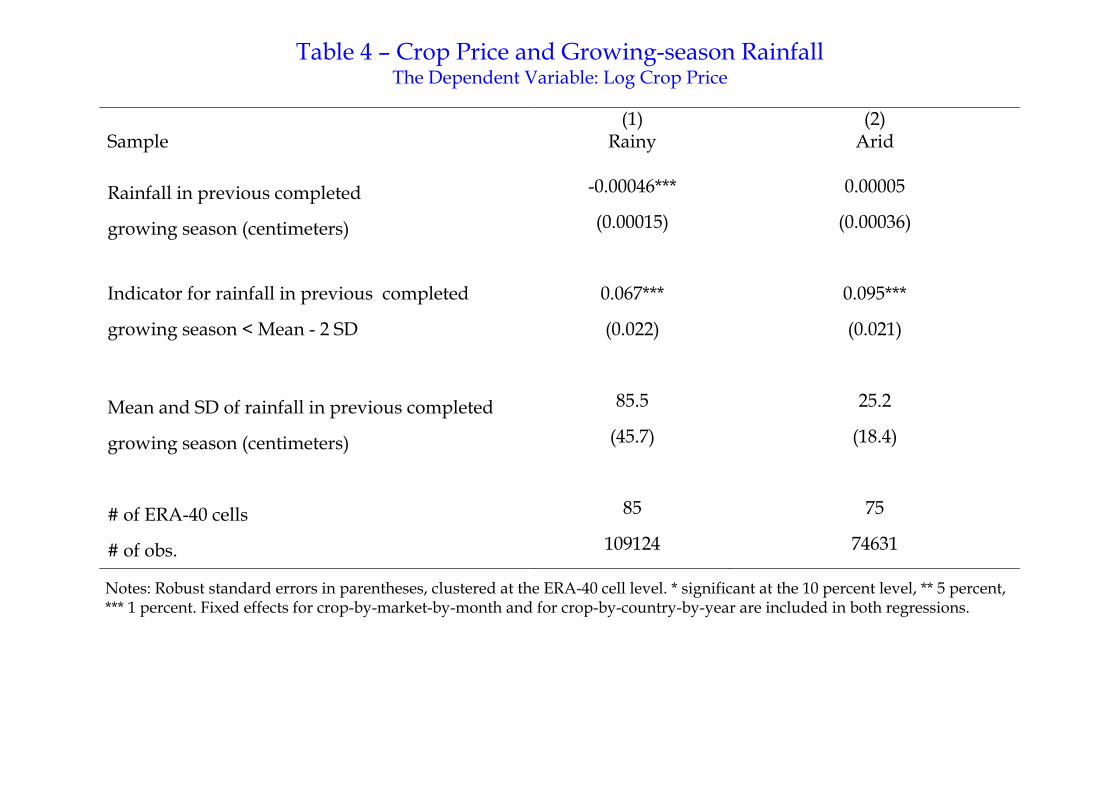
Table 4 reports the estimation results. Column (1) shows that in rainy

areas the crop price drops significantly by 2.1 percent with a one standard

deviation increase in rainfall during the previous completed growing season,

i.e., 1 in equation (3). A drought incident significantly increases the crop

price by 6.7 percent. Column (2) shows that in arid areas the linear impact of

growing-season rainfall on crop prices is insignificant, but a drought incident

significantly raises crop prices by 9.5 percent. These results give support to

our assumption that local rainfall affects the availability of food due to the

lack of irrigation and transportation infrastructure.

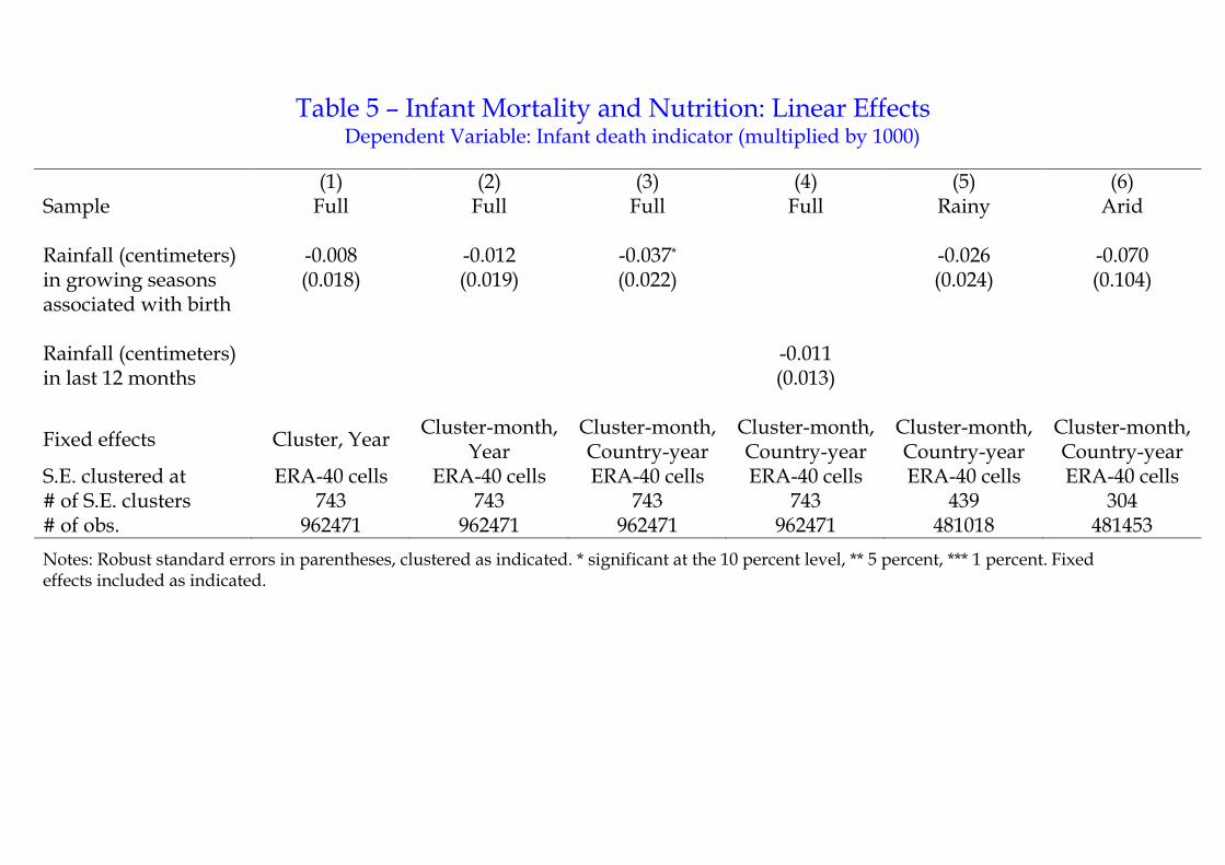
Basic results Table 5 reports the estimates from running panel regressions

like (2) in Section 3, except that we replace the malaria exposure index with the rainfall exposure index . Columns (1)-(3) show the estimates of

the coefficient of interest in the full sample, with only cluster fixed effects

or cluster-by-month fixed effects included, and with different treatment of

trends. The point estimates always have the expected negative sign — i.e.,

more rainfall in the growing season(s) before birth cuts the risk of infant

mortality. In the most conservative specification with country-specific non-

parametric trends in Column (3), the coefficient is the highest in absolute

value and is significantly different from zero at the 10% level.

Column (4) shows that the point estimate is lower in absolute value and

not significantly different from 0, if we replace with the cumulated rainfall

over the 12 months preceding birth, with no allowance for the location-specific

growing seasons. This indicates that our rainfall exposure index, following

from the first two assumptions underlying Definition 2, captures the mothers’

nutritional intake better than 12-month average rainfall.

Columns (5) and (6) report corresponding estimates when the same spec-

ification is estimated on the subsamples of babies born in rainy and arid

climate zones, respectively. In both areas, the point estimates have the same

negative sign as in the full sample, but are too noisy to be statistically sig-

nificant.

Non-linear effects: droughts and floods Since infant death is an ex-

treme health outcome, it is plausible that it is closely related to extreme

28

precipitation events, such as droughts or floods — in analogy with the malaria

epidemics discussed in Section 3. The linear specifications estimated in Table

5 do not allow for disproportional effects of extreme events, however.

We use a drought index based on extreme growing season rainfall out-

comes, defined as follows.

Definition 3 In each grid cell, we first compute the average value of our

rainfall exposure index, as well as its standard deviation, using the

full 45 years of ERA-40 data from 1957 to 2002 (irrespective of whether

we observe child births or not). We then define a binary drought indicator

variable for babies born in location and running month by

= [ − 2] . (4)

That is, the birth is associated with a drought indicator of unity if its

rainfall exposure index falls two standard deviations below the local mean.

For convenience, we define a flood symmetrically, as an extreme event in the

opposite direction.35

Table 6 displays the results from adding the drought and flood indexes

defined above to the econometric specification used in Column (3) of Table

5. The full-sample estimates in Column (1) — in the most conservative speci-

fication with cluster-month plus country-year fixed effects — show a positive,

albeit statistically insignificant, point estimate for drought and an insignifi-

cant, negative estimate for floods. The results for rainy areas in Column (2)

are similar.

In arid-area sample, the results are different. While the rainfall coefficient

in Column (3) is insignificant, as in Table 5, the estimated coefficient on

drought is positive and precisely estimated. The effect of a drought is now

estimated to be quite powerful: it raises infant mortality by 23.1 per 1000,

an amount equal to nearly a quarter of the sample mean. But we do not find

any effect of extreme positive amounts of rainfall.

The remaining three columns in Table 6 check the robustness of the result

in Column (3) in an analogous way to Columns (4)-(6) in Panel B of Table 2.

35Our drought measure is similar to the Standardized Precipitation Index (McKee et

al., 1993), but is based on our rainfall exposure index rather than just average rainfall. For

a discussion of drought indices and their application to Africa, see Ntale and Gan (2003).

We also interacted our drought index with the indicator of vulnerability to drought and

flood from Dilley et al. (2005). However, this interaction variable did not significantly

affect infant mortality.

29

Column (4) shows that these estimates for arid areas are robust to clustering

the standard errors at climate zones by 5-year periods.36 In Column (5), we

add cubic polynomials in the past 12-month temperature and rainfall to the

regression, and obtain a similar point estimate for droughts. Finally, Column

(6) adds ERA-40 cell specific linear trends and obtains a point estimate

almost identical to that in Column (3).

Figure A3 in the Appendix shows all the ERA-40 cells which experience

at least one incidence of drought for months in which we observe births in the

sample, analogous to Figure A2 mentioned in Section 3. As seen from the

figure, the droughts from which we identify our estimates are quite evenly

spread over the various African regions that make up the arid climate zone

of our sample.

Taken together, our results suggest that in arid areas extreme shortfalls of

rain have large effects, while more piecemeal variations in precipitation do not

have any measurable effects on infant mortality. These results are consistent

with Susser (1991), who reviews studies on the relationship between maternal

nutrition and birth weight and concludes that nutritional intake by mothers

significantly affects birth weight only in famine conditions.

In Section 5, we use these results to estimate historical death tolls due to

drought, and discuss implications of climate change.

Heterogeneity by household characteristics? The specifications in Ta-

bles 5 and 6 do not allow for any heterogeneous effects across households,

mothers and babies (beyond a difference across climate zones). We now

turn to these issues. It is natural to believe that the vulnerability of the

offspring to maternal malnutrition might differ with mother or household

characteristics, such as occupation, income, or education. Table 7 presents

some estimates relevant to this hypothesis. We focus on two specific sources

of heterogeneity, which appear important a priori and reasonably measurable

in the DHS data. One is occupation: we call an infant’s household agricul-

tural, when the parents earn a living only from agriculture at the time of the

survey. In the full sample, about 42% of all children, excluding those with

missing information on their parents’ occupation, are born in agricultural

households. Measurement error in the classification of agricultural house-

holds is inevitable: parents may have changed the job since the baby’s birth,

36The arid areas are divided into 4 zones by northern versus southern hemispheres and

by steppe versus desert climate zones, as defined by the Köppen climate classification.

30

and the definition of agriculture in the DHS data also includes forestry and

fishery. These factors, however, would bias our results against finding het-

erogeneous effects of weather fluctuations.

We also consider education, and define a baby’s household as well-educated

if both the baby’s mother and her husband (if relevant) have more than eight

years of education. Eight years is chosen as the cutoff, because we see a

marked drop in the cross-sectional distribution of infant mortality above this

level of education. In the DHS sample, only slightly more than 8% of the

babies are born to well-educated households. The retrospective nature of the

survey is unlikely to be a major source of mismeasurment when it comes to

education. See Table 1, Panel A for summary statistics by subgroup.

We then run the following regression:

= + · + + · (5)

+ + · + +

· + ,

where is an indicator of baby ’s household type (agricultural or well-

educated). Note that this specification allows cluster-by-month and country-

by-year fixed effects to differ across different household types. Table 7 reports

the estimated coefficients: , , , and .

Column (1) shows the estimates for the occupational breakdown in the

rainy sample. In contrast to the results in Tables 5 and 6, the results suggest

that rainfall exerts a significant negative linear effect on infant mortality if we

look at agricultural households. The sum of the two coefficients on rainfall

( + ) — the total linear effect of rainfall for agricultural households — is

statistically significant at the 5 percent level. The non-interacted coefficient

() shows that the effect is statistically insignificant and close to zero for

non-agricultural households. To the contrary, droughts have no effect on

infant mortality in either groups in rainy areas.

In arid areas, the results in Column (2) show something close to the op-

posite. There is no linear effect of rainfall on infant mortality in either group.

But a drought has a large effect in non-agricultural households, whereas it

has no significant effect in agricultural households (the sum of and is

not significantly different from zero).

A reasonable interpretation of these results is that in rainy areas a normal

downward variation in rainfall tends to make agricultural households worse

off nutritionally. On the other hand, in arid areas such households have better

access to whatever little crop yield there may be at the time of drought, so

the main burden is instead borne by non-agricultural households.

31

Columns (3) and (4) repeat the same exercise for the breakdown of house-

hold type by education. The main result here is two-fold. It is primarily the

non-educated that benefit from more rainfall in rainy areas. And — as might

be expected — the well-educated appear to be protected from the high in-

fant mortality effects of a drought shock in arid areas, perhaps as a result of

higher purchasing power or better opportunities.

As in the malaria section, we have also experimented with conditioning on

various baby and mother characteristics (gender, birth order of child, age or

stature of mother, etc.), on the notion that some types of babies or mothers

may be more vulnerable to malnutrition shocks than others. But this has

produced no robust results.

Heterogeneity by timing of birth As mentioned after Definition 2, our

simple rainfall and drought exposure indexes implicitly assume that the mar-

ginal effects on infant mortality are constant across time. We now relax this

assumption by conditioning the effects of shocks on the time of birth relative

to the beginning of the growing season. Given the earlier results, we focus

on the drought effects in arid areas and run the regression:

=

3X=0

· +3X

=0

· + + + , (6)

where is a dummy that equals one if calendar month of date falls

within the th quarter since the beginning of the growing season in grid

( = 0 for the quarter immediately before the growing season starts).

Figure 8 plots estimated coefficients of the s and their 95% confidence

intervals. The vertical line in the figure indicates the beginning of the growing

season — recall Figure 6 and our definition of this as the time when the NDVI

value is 20% above its last trough. The babies born in the quarters around

the beginning of the growing season, marked 0 and 1 in Figure 8, seem to

fare much worse in the wake of a drought shock than the babies born closer

to the harvest. The estimated hike in death rates for these babies — on the

order of 60 per 1000 births — is a stunning number indeed.

These results are related to the notion of a “hungry season”, in the lit-

erature on food availability and poverty. The average length of the growing

season in arid areas is about 6 months in our sample, and the actual harvest

may start before the end of the fixed growing season we use in the analysis.

32

Therefore, food is the least available in the period around (in particular, af-

ter) the beginning of the growing season. On top of that, the beginning of

the growing season is the time when energy expenditure of people — includ-

ing pregnant women — reaches its peak over the year owing to the need for

clearing the land and planting the seeds.

A study on pregnant women in a Gambian village shows that pregnancy,

even in the last month before giving birth, does not reduce the time women

spend at their farms (Roberts et al. 1982). Studying the same rural area

in Gambia, Rayco-Solon et al. (2005) find that the incidence of premature

birth (a major cause of low birth weight) significantly increases during the

first few months of the rainy season, which suggests a possible causation from

increased amount of workload for pregnant women to low birth weight.

Moreover, we can compare the estimated effects of random variations in

rainfall with the results from randomized controlled trials which vary nu-

tritional intakes in other ways. Thus, in one study, a treatment group of

randomly selected pregnant women in Gambia were given dietary supple-

ments (Ceesay et al., 1997). According to that study, the effect of these

supplements on the incidence of low birth weight and early infant death were

both significantly larger for babies born in the hungry season. Our empiri-

cal findings suggest that these results from particular Gambian villages may

likely be generalized to a much greater arid area of Africa.

Malaria and malnutrition We have investigated separately two channels

whereby local seasonal weather shocks affect infant mortality rates in Africa.

While we have carefully defined these weather shocks according to the mech-

anism under investigation, all the shock measures emanate from the same

weather data. It is thus legitimate to ask if the results hold up when we al-

low both types of shocks to occur simultaneously. For example, more rainfall

can potentially have two opposite effects on infant mortality: more rain may

be good through increased nutrition but bad through increased malaria. For

the babies in our sample, the malaria exposure index is indeed positively

correlated with the rainfall exposure index with a correlation coefficient

in the full sample of 0.76.

The brief answer is yes. As shown in a previous version of the paper,

a few of the point estimates for the linear effect of growing season rainfall

and the number of malaria months increase in absolute value. But all the

important estimates of nonlinear effects — of malaria epidemics and droughts

33

— are not affected.

Summary Let us briefly summarize the message of this section. Extreme

negative rainfall shocks (droughts) have a powerful effect on infant death

in areas with steppe and desert climates. Rainfall above the site-specific

seasonal mean in the relevant growing season diminishes infant mortality

only for babies born in agricultural households in the rainy parts of Africa.

Drought shocks impinge especially hard on babies to parents that do not

work in agriculture, are not well educated, and on babies born around the

start of the rains.

5 Aggregate Effects and Methodology Issues

What can our results say about aggregate effects of weather on infant mor-

tality? In this section, we first estimate how many infant deaths during (part

of) our sample period were caused by extreme malaria episodes in epidemic

areas and by drought episodes in arid areas. Second, we estimate how many

infants deaths in all of Africa are caused by malaria in epidemic regions and

by droughts. We compare the resulting figures to existing estimates and dis-

cuss methodological differences. Finally, we try to pinpoint areas at risk for

high infant mortality at the end of this century, given a distribution of future

weather implied by simulations of general circulation models with a changing

climate due to continued emissions of carbon dioxide.

Aggregate effects of malaria epidemics and droughts What is the

excess infant mortality due to malaria epidemics across all epidemic regions

of Africa? To answer this question, we begin by estimating the expected

number of births for each year and ERA-40 cell in the epidemic regions of

Africa, during the subperiod for we which we have reliable gridded population

data, namely 1981-2000.37 We then multiply the estimated number of births

37We start with the Gridded Population of the World version 3 (CIESIN and CIAT

2005) to obtain the population count in each 2.5 by 2.5 arc minute cells in 1990, 1995 and

2000. Next, we aggregate this number to the intersections of the ERA-40 cells and country

boundaries. We then linearly interpolate the population at the intersection level for years

in the 1990s. For years before 1990, we use the country-level population growth from the

World Development Indicators (WDI; World Bank 2012) to extrapolate population counts.

Finally, we use the country-level crude birth rate from the WDI to obtain the number of

34

with the increase in the probability of infant death in events with three or

more malaria months above the average, implied by the estimates in Columns

(3) and (7) of Table 3. This yields the excess infant mortality caused by each

such malaria episodes. Finally, we sum the excess infant mortality across all

these malarious episodes.

If we restrict attention to the ERA-40 cells in our sample, then the total

excess deaths caused by these malarious episodes during 1981-2000 is 84,000

out of 139 million births. Extrapolating to all malaria epidemic areas of

Africa — which are shown in Figure A4 of the Appendix — we estimate that

106,000 infants died in these malaria episodes out of 179 million births in the

same twenty years. This is 0.64 children in 1000 births, accounting for a bit

less than 1 percent of infant mortality.

Analogously, we estimate the excess number of infants dying of droughts

in Africa’s arid climate zones. The calculation now relies on the estimate

in Column (6) of Table 6. In the sample areas, we estimate an 8,700 extra

infant deaths from these droughts, out of 141 million births. Extrapolating

to all arid areas of Africa — shown in Figure A5 — we estimate 11,000 extra

infant deaths, relative to 206 million births. This is only 0.05 children in

1000, accounting for 0.05 percent of infant mortality. The reason that these

additional death tolls are relatively small is of course that the underlying

extreme events are infrequent.

Total number of infant deaths from malaria We can also estimate the

total number of infant deaths caused by malaria in the epidemic regions. Our

estimate is based on the fall in infant mortality when there are zero malarious

months in the year before birth relative to a typical year. This estimate is

in the same spirit as comparing infants of mothers randomly assigned to

malaria medicine treatment (and for this reason non-malarious) with infants

of mothers not given treatment (see below). In our study, because of random

weather fluctuations, some mothers were non-malarious and our estimate

compares their infants to infants born under normal malarious conditions

in this area. Note that we cannot similarly estimate the effect of a long-

term reduction of malaria from an average 2-4 months to an average of 1-2

malarious months based on the estimates in Table 3. The reason is that

adaptation (for example, partial immunity to malaria) would change. We

can, however, estimate that change by comparing the effects of a drop to

births in each year and then aggregate it to the ERA-40 cell level.

35

zero malaria in the two regions.

In areas with 2-4 average malaria months, our estimates (column (8) in

Table 3) imply that infant mortality drops by 8.1 deaths per 1000 when there

are zero malarious months in the year before birth relative to the average

year. Since the average infant mortality rate in these areas is 108.9 per 1000,

malaria is estimated to account for 7.4% of infant mortality (95% confidence

interval is 4-11%). We multiply this number by the total number of births in

a year to get the reduction in infant mortality from eliminating malaria. We

find that 629,000 infant lives out of 64 million births were lost due to malaria

in these epidemic regions in 1981-2000. In areas with 0-2 average malarious

months, our point estimate of a drop to zero malaria is not significantly

different from zero.

Existing studies of infant deaths from maternal malaria How do

these estimates of infant death in malaria compare with existing medical

studies? Mortality estimates ideally come from national vital registration

systems that categorize all deaths in the country by cause. However, such

systems do not exist for most African countries.

Existing medical studies therefore use two types of alternative data sources.

The first is epidemiological surveys, including randomized control trials, on

the impact of medical treatment of malaria infection.38 The second is ver-

bal autopsy reports, which attempt to assign cause of death based on signs,

symptoms and events leading up to the death as reported by caretakers of the

deceased and sometimes supported by medical documentation. Both types of

data, however, come from a limited number of selected populations in Africa.

We now compare our methodology with that used in studies using each

type of data sources.

Epidemiological surveys The existing study based on epidemiological

surveys with a scope most comparable to our own is probably Steketee et al

(2001). These authors review studies on malaria infection in pregnancy and

estimate that 3-8% of infant mortality in endemic areas is due to malaria

38There also exist some randomized control trials on the prevention of malaria.

Insecticide-treated bed nets are, for example, estimated to reduce infant mortality by

an average 5.5 deaths per 1000 births, according to five studies in endemic areas of sub-

Saharan Africa (Lengeler, 2004). Preventive measures against malaria such as bed nets,

however, only partially reduce malaria incidence and for this reason provide a lower bound

on the effect of eliminating malaria.

36

in pregnancy. Of 34 reviewed studies, only two attempt to estimate the

contribution of malaria to infant mortality, namely Greenwood et al. (1992)

and Steketee et al. (1996). Both studies are unable to directly estimate the

effect because sample sizes are not large enough to estimate effects on such

rare events as infant deaths. Instead, both studies first estimate the effect

of malaria medicine on birth weight by using a randomized control trial, and

then combine this estimate with the correlation coefficient between low birth

weight and infant mortality based on observational data. In the words of

Steketee et al. (2001), “No study has made the direct observation because

the required sample size to make the observation is prohibitively large.” This

issue is of course even more pronounced in non-endemic areas, which explains

the paucity of epidemiological studies there.

Specifically, Greenwood et al. (1992) study villages near the town of

Farafenni on the north bank of the Gambia river and finds that malaria

medication could reduce infant mortality by 6% (from 50 to 48 per 1000).

Stekeete et al. (1996) study women enrolled in four antenatal clinics in

a highly endemic malaria area of rural Malawi and estimate the effect of

malaria to 3-5% of infant mortality, at an average infant mortality rate of

157 per 1000. Steketee et al. (2001) summarize these estimates and adjust

the summary estimate to an upper limit of 8%, to account for effects through

anemia. Scaling the effects by regional infant mortality rates, the paper

finds that globally, 75,000 to 200,000 infant deaths in each year might be

attributable to malaria infection during pregnancy.

A number of assumptions are necessary to draw these conclusions. In

order to consistently estimate the effects of malaria on infant mortality in

a studied population, one has to assume that: (E1) no factor correlated

with birth weight directly affects infant mortality and (E2) malaria affects

infant mortality only through birth weight. To extrapolate to other areas and

times, additional assumptions are required: (E3) effects are proportional to

the average infant mortality rate in the region and (E4) the level of malaria

exposure in the regions and times of the study are representative of all regions

and times.

In comparison, our estimates rely on random year-to-year weather shocks

to identify effects on infant mortality. Consequently, our random assign-

ment depends on weather fluctuation rather than explicit randomization (or

assignment by day as in Stekeete et al. 1996). Because of the very large sam-

ple size of our data set (nearly a million births), we can estimate the effect

on infant mortality directly and do not have make assumptions such as (E1)

37

and (E2) to draw conclusions. Our sample is also a lot more representative

of all of Africa during the sample period, and we measure the average effect

across this sample. For this reason, we do not have to make assumptions

(E3) and (E4) to extrapolate our results to other regions and times.

Verbal autopsy reports We now turn to studies based on verbal autopsy

reports. The estimates of malaria’s contribution to mortality of children

aged below 5 in the WHO’s World Malaria Report are based on results from

meta-regression studies. For example, Morris et al. (2003) use data from 38

verbal autopsy studies (14 in Africa) to establish the cause of death. The

share of deaths in each study attributed to each of five causes (relative to the

share attributed to pneumonia), is regressed on a number of characteristics.

The ratio of malaria to pneumonia deaths, for example, is regressed on the

estimated population at risk of malaria based on a model similar to ours

(the MARA model), the proportion of births attended by a qualified profes-

sional, access to safe drinking water, and a South Asia dummy variable. The

regression coefficients are then used to predict the distributions of under-5

deaths by cause for the entire region of Africa. Using this methodology, the

study concludes that 24 percent of child deaths in sub-Saharan Africa are

caused by malaria. Later studies such as Johnson et al. (2010) and Black et

al. (2010) reach similar numbers based on a larger number of verbal autopsy

studies. For Africa as a whole, these authors attribute 16% of under-5 deaths

to malaria.

While such cross-sectional regressions may predict the relative importance

of mortality causes, there are concerns about their ability to identify causes

of deaths. Three obvious ones are: (V1) cross-sectional correlations may

reflect confounding factors, (V2) errors in the verbal autopsy reports correlate

with the regressors, (V3) children may die of multiple illnesses, and deaths

due to malnutrition are assigned to other causes. Regarding (V1), many

omitted factors, like agricultural production, may correlate with the malaria

index in the cross-section. With respect to (V2), verbal autopsy may poorly

differentiate malaria from other diseases that cause fever symptoms (e.g.,

septicaemia, viral encephalitis or pneumonia), and thus fever may more likely

be seen as a sign of malaria in endemic areas. This alone would create a

correlation between malaria assigned as a cause of death and the population

at risk of malaria, biasing the estimated coefficient on this factor.

Concerning (V3), extrapolating to the effects of eliminating malaria is not

38

straightforward. The verbal-autopsy methodology is designed to predict the

relative importance of mortality causes, not the absolute number of deaths,

which is taken as exogenous. On one hand, as children die of multiple ill-

nesses, eliminating malaria may reduce vulnerability to other illnesses. On

the other hand, weak and vulnerable children, whose deaths are attributed

to malaria, may increasingly die of other causes when malaria is eliminated.

In comparison to the meta-regressions based on verbal autopsy reports, we

use random time series variation within the same locality to identify effects.

Confounding cross-sectional variation is thus absorbed by our cluster-by-

month fixed effects to avoid concern (V1) — a key motivation for our choice

of methodology. Also, we do not rely on verbal autopsy reports and hence we

capture the effect on total infant mortality directly, avoiding concerns (V2)

and (V3).

Existing studies of malnutrition and infant mortality Our results

on how weather influences infant deaths are supported by the fact that, in

arid areas, the same weather pattern (droughts) that influences crop prices

(and thus likely nutrition) also affect infant mortality. How do they compare

with existing research on the effects of malnutrition on infant mortality? Let

us compare our aggregate estimate of 11,000 infant deaths due to droughts

in 1981-2000 with numbers from the EM-DAT data base of the Centre for

Research on the Epidemiology of Disasters. This data records 195 droughts

in Africa 1981-2000, involving a total of 554,756 killed. Assuming that infants

make up 3% of the population (from the WDI crude birth rate), and that

all ages are hit uniformly, this would imply 16,600 excess infant deaths due

to drought over the twenty-year period. However, a uniform distribution

of mortality risk across ages may not be realistic. De Waal (1989) found

that infants were less affected by Sudan drought in 1984-1986 than average,

because of late weaning.39 Similarly, Ezra and Kiros (2000) find that infants

were less affected by the Ethiopia drought in 1984-1985.

But the vast majority (99%) of the deaths recorded by EM-DAT are

39De Waal conducted a survey of 1182 households in Sudan in 1986, investigating the

second deadliest drought in our sample period. He found that infant mortality was not

higher during the drought 1984-1986 than typical, although infant deaths may have been

under-enumerated. He argues that a reason that infants were protected from the drought

was habits of late weaning. The infants were less vulnerable to many of the diseases

associated with unclean water supplies or inferior foods, and had the protection against

infection provided by their mothers’ milk.

39

associated with a mere three droughts in the mid 1980s (Ethiopia, Sudan

and Mozambique). Our mortality toll is much more dispersed in time and

space. It captures a different phenomenon: extreme deviations from local

rainfall conditions in arid areas that typically do not attract the attention of

the large aid donors. Interestingly, the estimated aggregate infant mortality

from these unnoticed disasters is of the same magnitude as that of the major

disasters entering in EM-DAT.

More generally, estimates of the relation between malnutrition and in-

fant mortality in existing studies are not directly comparable to ours. One

common approach is to use meta-regressions of (the log of) average infant

mortality rates by weight-for-age categories on weight for age. The distribu-

tion of infant weight for age in the data is then used to compute the excess

mortality relative to the ideal weight for age (see Pelletier 1994 and Black et

al. 2008 for examples). A typical estimate is that one half to one third of

infant mortality is attributable to malnutrition and that mortality increases

monotonically as weight falls, at least in a region from one standard deviation

below the mean. When such studies are used to predict infant mortality lev-

els, they may not capture the causal effect of malnutrition on child mortality.

In particular, social and disease related factors may affect both malnutrition

and infant mortality. Thus, we cannot readily use results from such stud-

ies to estimate the causal effect, through nutrition, of weather variations or

climate change on infant mortality.

Another approach is to rely on randomized experiments to assess the ef-

fect of nutrition on child mortality. Kramer and Kakuma (2003) review the

evidence on energy and protein intake in pregnancy and conclude that bal-

anced energy/protein supplements improve fetal growth and may reduce the

risk of fetal and neonatal death. Ceesay et al. (1997), mentioned above, find

large effects on fetal growth and mortality. However, this particular study

provided much higher energy supplements than typical to under-nourished

women from Gambia. To exploit results like these to estimate the effect of

weather variation on infant mortality, one needs to know how the distribu-

tion of nutrient consumption across Africa changes with weather variations,

and the average response of infant mortality to these changes.

Areas at risk and their evolution over time We have identified the

African areas most vulnerable (in terms of infant survival) to weather shocks,

namely epidemic malaria zones and arid climate zones. What can we say

40

about areas at risk when the climate changes? As a lead-in to this question,

we can ask if the location of vulnerable areas has changed during the past

three decades, possibly due to ongoing climate change. For this purpose, we

split the 28-year period from September 1974 to August 2002 in half and

classify ERA-40 cells into different malaria zones and climate zones in each

subperiod.

Appendix Figure A6 shows where malaria zones shifted (and the average

number of malaria months per year changed by one or more) from the first

subperiod (before 1988) to the second (after 1988). Some of the areas just

south of the Sahel region became less malarious, while some areas in eastern

and southern Africa became more malarious.40 Similarly, Appendix Figure

A7 shows where the climate zone shifted between arid and rainy areas.

Now we turn our attention to the implications of our findings on the possi-

ble impacts of climate change in the future. Projections of future climate in-

dicate that Africa will get significantly warmer. Areas hitherto non-malarious

due to cold temperature — mountainous regions in Ethiopia, Kenya, Mada-

gascar, and Zimbabwe close to the yellow dots in Figure 5 — are thus likely

to become new epidemic areas, where mothers will have little immunity and

infants will be very vulnerable to temporary malaria epidemics. Moreover, if

future climate change leads to more dramatic variations in the annual fluctu-

ations of rainfall in the drier parts of Africa, this too will shift the distribution

of malaria exposure — epidemics may become more frequent in low-prevalence

areas, with potentially large effects on infant mortality. [We are currently

obtaining climate predication data to be more precise about these

future patterns. Specifically we will create maps similar to Figures

A6 and A7 of the areas that may become more or less malarious,

and arid or rainy, in the last three decades of the 21st century

compared to our sample period.]

To further illustrate these possibilities, Figure A8 shows whether the epi-

demic episodes we identify in sample are mainly caused by higher tempera-

ture or larger precipitation.41 Epidemic episodes in Ethiopia and Kenya are

40This observation is consistent with papers that point to a resurgence of malaria in the

East African Highlands from the mid 1980s, typically citing evidence that derives from a

small number of clinics (see e.g., Hay et al. 2002) or verbal autoposies.41For each ERA-40 cell and month where the number of malaria months in the past

12 months contain an epidemic, we check whether the past 12-month average monthly

temperature and precipitation are higher than the 1957-2002 average. If only temperature

(precipitation) accounts for at least 90% of the epidemic months in a given cell, we say that

41

mostly caused by larger-than-usual precipitation. This is consistent with the

notion that El Nino episodes are associated with wetter condition in East

Africa (recall Section 2). That the epidemics are mainly driven by rainfall

illustrates how larger fluctuations of rainfall in a future climate may lead to

more frequent malaria epidemics. On the other hand, the epidemic episodes

in Zambia are mostly caused by higher temperature than usual. This illus-

trates the possible epidemics caused by a higher frequency of warm enough

weather as the climate gets generally warmer.

To make this discussion more precise, we use the data on predicted

monthly temperature and precipitation for the period 2071-2100.42 We use

these data to identify the areas of Africa that will become more vulnerable

to weather shocks in terms of infant survival by becoming an epidemic area

or an arid area (or by a higher frequency of malaria epidemics and droughts

in areas that are already epidemic or arid). We then use our estimates in the

paper to estimate how many infants may be expected to die due to certain

types of weather shocks at the end of the 21st century.

[Results and discussions to be inserted here.]

6 Final Remarks

We believe this paper makes substantive as well as methodological contribu-

tions.

In terms of substance, we uncover two main channels whereby weather

shocks impact infant mortality in African countries. Weather shocks that

raise malaria exposure of pregnant mothers have a large impact on infant

death, especially when they sow the seeds of a malaria epidemic in areas

where malaria is rare. Drought shocks have a pronounced effect on infant

death in arid areas, especially for babies whose parents are not well educated,

not dependent on agriculture, and for babies who are born in the hungry sea-

the episodes are predominantly caused by temperature (precipitation). This is indicated by

orange (blue) in the figure. If both temperature and rainfall, or neither of the two, explain

at least 90% of the epidemic episodes, we regard epidemics caused by both, indicated by

yellow in the figure.42We use the climate prediction data derived from the EC-EARTH model, the climate

model closest to the one used in the ERA-40 reanalysis, and based on two emission scenar-

ios under the CMIP5 (Climate Model Intercomparison Project phase 5) project: a high

emissions scenario (RCP8.5) and a midrange mitigation emissions scenario (RCP4.5). See

Taylor et al. (2012) for the detail on the CMIP5.

42

son. The malaria epidemic and drought effects we estimate are statistically

robust and quite large.

The continental scale in our study leads to a bleak picture for certain parts

of Africa, especially in some areas with scant rainfall that also suffer from

bursts of epidemic malaria, such as the mountainous areas in East Africa.

Due to the erratic movements of the Intertropical Convergence Zone, these

areas face large variations in annual rainfall. When it rains a lot this may

cause a malaria epidemic, when it rains a little this may cause a drought —

whichever way with bad outcomes for infant mortality. We have also shown

how to use our results to estimate the total number of infant deaths due to

maternal malaria in epidemic areas.

In terms of methodology, we have outlined a possible research design for

impact research, showing how one may combine very different data sources

for large-scale statistical work, when conventional data sources are absent or

poor. We have also shown how this methodology allows us to draw reasonable

conclusions about the aggregate impacts for all of Africa in the past few

decades.

We have also indicated how some of our results could be used to identify

areas at risk for large future health impacts in the wake of future climate

change. [Say more in light of the, now missing, results] On this front,

much more work is needed to come up with more robust conclusions.

A similar approach and statistical methodology may be used to study

other outcomes of interest in Africa or other regions. For example, further

research on Africa could use DHS data to look at the weather dependence

of other outcomes, such as child mortality, child health, or fertility. Perhaps

one may also study more complex issues, such as generational spillovers,

whereby girls with negative weather shocks in early life become physically or

cognitively impaired adults and thus face a larger risk of bad outcomes when

they give birth themselves.

There is certainly scope for improvement on the natural-science side of our

measurement. For example, one could try to use re-analysis from regional

rather than global climate models to obtain more recent and fine-gridded

weather data, so as to better pick up the spatial distribution of rainfall. As

another example, one could try to use structural crop-yield models to get a

better handle on the interplay between temperature and rainfall in producing

local crop yields.

These and other tasks are left for future research.

43

References

[1] Artadi, Elsa V. 2006. “Going into Labor: Earnings vs. Infant Survival

in Rural Africa.” Unpublished manuscript.

[2] Auffhammer, Maximilian, Solomon M. Hsiang, Wolfram Schlenker, and

Adam Sobel. 2011. “Global Climate Models and Climate Data: A User

Guide for Economists.” Unpublished manuscript.

[3] Bantje, Han. 1983. “Seasonal Variations in Birthweight Distribution in

Ikwiriri Village, Tanzania.” Journal of Tropical Pediatrics, 29(1): 50

-54.

[4] Barecca, Alan et al. 2012. “Adapting to Climate Change: Evidence from

Long-Run Changes in the Weather-Mortality Relationship in the 20th

Century United States.” Mimeo.

[5] Black, Robert E et al. 2008. “Maternal and Child Undernutrition:

Global and Regional Exposures and Health Consequences.” Lancet,

371(9608): 243-260.

[6] Black, Robert E et al. 2010. “Global, regional, and national causes of

child mortality in 2008: a systematic analysis.” Lancet, 375(9730): 1969—

1987.

[7] Brabin, Bernard J. 1983. “An Analysis of Malaria in Pregnancy in

Africa.” Bulletin of the World Health Organization, 61(6): 1005-1016.

[8] Brabin, Bernard, J. et al. 2004. “The Sick Placenta — The Role of

Malaria.” Placenta, 25(5): 359-378.

[9] Brown, K. H., and Kathryn G. Dewey. 1992. “Relationships Between

Maternal Nutritional Status and Milk Energy Output of Women in De-

veloping Countries.” In Mechanisms Regulating Lactation and Infant

Nutrient Utilization, eds. M. F. Picciano and B. Lönnerdal. New York:

Wiley-Liss, pp. 77-95.

[10] Bruckner, Markus, and Antonio Ciccone. Forthcoming. “Rain and the

Democratic Window of Opportunity.” Econometrica.

44

[11] Burgess, Robin, Deschenes, Olivier, Donaldson, David and Michael

Greenstone. 2010. “Weather and Death in India: Mechanisms and Im-

plications of Climate Change.” Unpublished manuscript.

[12] Ceesay, Sana M et al. 1997. “Effects on Birth Weight and Perinatal

Mortality of Maternal Dietary Supplements in Rural Gambia: 5-year

Randomised Controlled Trial.” British Medical Journal, 315(7111): 786-

790.

[13] CIESIN and CIAT. 2005. Gridded Population of the World, Ver-

sion 3 (GPWv3). Palisades, NY: Socioeconomic Data and Ap-

plications Center (SEDAC), Columbia University. Available at

http://sedac.ciesin.columbia.edu/gpw.

[14] Chambers, Robert, Richard Longhurst, and Arnold Pacey, eds. 1981.

Seasonal Dimensions to Rural Poverty. London: Pinter.

[15] Climate Research Unit. “Advice for Time-Series Analysis.” Available at:

http://www.cru.uea.ac.uk/ timm/grid/ts-advice.html [Accessed August

20, 2010].

[16] Desai, Meghna et al. 2007. “Epidemiology and Burden of Malaria in

Pregnancy.” Lancet Infectious Diseases, 7(2): 93-104.

[17] Deschenes, Olivier, and Michael Greenstone. 2007a. “The Economic Im-

pacts of Climate Change: Evidence from Agricultural Output and Ran-

dom Fluctuations in Weather.” American Economic Review, 97(1): 354-

385.

[18] Deschenes, Olivier, and Michael Greenstone. 2007b. “Climate Change,

Mortality, and Adaptation: Evidence from Annual Fluctuations in

Weather in the US.” Unpublished manuscript.

Dilley, Maxx et al. 2005. Natural Disaster Hotspots: A Global Risk

Analysis. Washington, DC: World Bank.

[19] DeWaal, Alex. 1989. “FamineMortality: A Case Study of Darfur, Sudan

1984—5.” Population Studies: A Journal of Demography, 43(1): 5-24.

[20] Ezra, Markos and Gebre-Egziabher Kiros. 2000. “Household Vulnerabil-

ity to Food Crisis and Mortality in the Drought-Prone Areas of Northern

Ethiopia”, Journal of Biosocial Science, 32(3): 395-409.

45

[21] Fallis, G, and John Hilditch. 1989. “A Comparison of Seasonal Variation

in Birthweights between Rural Zaire and Ontario.” Canadian Journal

of Public Health, 80(3): 205-208.

[22] Frenken, Karen, ed. 2005. Irrigation in Africa in Figures: AQUASTAT

Survey, 2005. Rome: FAO.

[23] Greenwood AM, et al. 1992. “Malaria chemoprophylaxis, birth weight

and child survival.” Transactions of the Royal Society of Tropical Medi-

cine and Hygiene, 86: 483—485.

[24] Griffiths, John F., ed. 1972. Climates of Africa. Amsterdam: Elsevier

Publishing Company.

[25] Guyatt, Helen L., and Robert W. Snow. 2004. “Impact of Malaria dur-

ing Pregnancy on Low Birth Weight in Sub-Saharan Africa.” Clinical

Microbiology Reviews, 17(4): 760-769.

[26] Guyatt, Helen L., and Robert W. Snow. 2001. “Malaria in Pregnancy

as an Indirect Cause of Infant Mortality in Sub-Saharan Africa.” Trans-

actions of the Royal Society of Tropical Medicine and Hygiene, 95(6):

569-576.

[27] Hay, S.I et al. 2002. “Climate Change and the Resurgence of Malaria in

the East African Highlands.” Nature, 415(6874): 905—909.

[28] Hay S.I. et al. 2009. “A World Malaria Map: Plasmodium Falciparum

Endemicity in 2007.” PLoS Medicine, 6(3): e1000048.

[29] Herbst, Jeffrey. 2000. States and Power in Africa: Comparative Lessons

in Authority and Control. Princeton, N.J.: Princeton University Press.

[30] Heumann, Benjamin W. et al. 2007. “AVHRR Derived Phenological

Change in the Sahel and Soudan, Africa, 1982-2005.” Remote Sensing

of Environment, 108(4): 385-392.

[31] Johnson, Hope L. et al. 2010, “Estimating the Distribution of Causes

of Death among Children Age 1—59 months in Highmortality Countries

with Incomplete Death Certification.” International Journal of Epidemi-

ology, 39: 1103—1114.

46

[32] Jönsson, Per and Lars Eklundh. 2004. “TIMESAT — A Program for

Analyzing Time-series of Satellite Sensor Data.” Computers and Geo-

sciences, 30: 833-845.

[33] Kiszewski Anthony and A. Teklehaimanot A. 2004. “A Review of the

Clinical and Epidemiologic Burdens of Epidemic Malaria.” American

Journal of Tropical Medicine and Hygiene, 70:128-135

[34] Kiszewski, Anthony et al. 2004. “A Global Index Representing the Sta-

bility of Malaria Transmission.” American Journal of Tropical Medicine

and Hygiene, 70(5): 486-498.

[35] Kinabo, Joyce. 1993. “Seasonal Variation of Birth Weight Distribution

in Morogoro, Tanzania.” East African Medical Journal, 70(12): 752-755.

[36] Kramer, Michael S. 1987. “Determinants of Low Birth Weight: Method-

ological Assessment and Meta-Analysis.” Bulletin of the World Health

Organization, 65(5): 663-737.

[37] Kramer, Michael S. and Ritsuko Kakuma. 2003. “Energy and protein

intake in pregnancy (Review)” Cochrane Database Syst Rev 2003; 4:

CD000032. DOI: 10.1002/14651858.

[38] Krasovec, Katherine, andMary Ann Anderson. 1991. “Maternal Anthro-

pometry for Prediction of Pregnancy Outcomes: Memorandum from

a USAID/WHO/PAHO/MotherCare Meeting.” Bulletin of the World

Health Organization, 69(5): 523-532.

[39] Kudamatsu, Masayuki. Forthcoming. “Has Democratization Reduced

Infant Mortality in Sub-Saharan Africa? Evidence from Micro Data.”

Journal of the European Economic Association.

[40] Le Hesran, Jean Yves et al. 1997. “Maternal Placental Infection with

Plasmodium Falciparum and Malaria Morbidity during the First 2 Years

of Life.” American Journal of Epidemiology, 146(10): 826-831.

[41] Lengeler C. 2004. “Insecticide-treated bed nets and curtains for pre-

venting malaria (Review)” Cochrane Database of Systematic Reviews,

2: CD000363. DOI: 10.1002/14651858.CD000363.pub2.

47

[42] Lobell, David B. et al. 2008. “Prioritizing Climate Change Adaptation

Needs for Food Security in 2030.” Science, 319(5863): 607-610.

[43] Luxemburger, Christine et al. 2001. “Effects of Malaria during Preg-

nancy on Infant Mortality in an Area of Low Malaria Transmission.”

American Journal of Epidemiology, 154(5): 459-465.

[44] Maccini, Sharon, and Dean Yang. 2009. “Under the Weather: Health,

Schooling, and Socioeconomic Consequences of Early-life Rainfall.”

American Economic Review, 99(3): 1006-1026.

[45] Maegraith, Brian. 1984. Adams and Maegraith: Clinical Tropical Dis-

eases. 8th ed. Oxford: Blackwell Scientific.

[46] McCormick, M C. 1985. “The Contribution of Low Birth Weight to

Infant Mortality and Childhood Morbidity.” New England Journal of

Medicine, 312(2): 82-90.

[47] McGregor, Ian A. 1984. “Epidemiology, Malaria and Pregnancy.” Amer-

ican Journal of Tropical Medicine and Hygiene, 33(4): 517-525.

[48] McKee Thomas B, Nolan J. Doesken, John Kleist, 1993. “The Rela-

tionship of Drought Frequency and Duration to Time Scales.” In Eighth

Conference on Applied Climatology, Anaheim, CA, 179-184.

[49] McKnight, Tom and Darrel Hess. (2000). Climate Zones and Types: The

Köppen System. Physical Geography: A Landscape Appreciation. Upper

Saddle River, NJ: Prentice Hall

[50] Miguel, Edward, Shanker Satyanath, and Ernest Sergenti. 2004. “Eco-

nomic Shocks and Civil Conflict: An Instrumental Variables Approach.”

Journal of Political Economy, 112(4): 725-753.

[51] Morris et al. 2003. “Predicting the Distribution of Under-five Deaths

by Cause in Countries without Adequate Vital Registration Systems.”

International Journal of Epidemiology, 32: 1041—1051.

[52] Murray, Christopher J. L., and Alan D. Lopez, eds. 1996. The Global

Burden of Disease: A Comprehensive Assessment of Mortality and Dis-

ability from Diseases, Injuries, and Risk Factors in 1990 and Projected

to 2020. Cambridge, MA: Harvard University Press.

48

[53] Mutabingwa, Theonest K et al. 2005. “Maternal Malaria and Gravidity

Interact to Modify Infant Susceptibility to Malaria.” Public Library of

Science Medicine, 2(12): e407.

[54] Ntale, Henry K. and Thian Yew Gan 2003, “Drought Indeces and Their

Application to East Africa”, International Journal of Climatology, 23,

1335-1357.

[55] Owens, Stephen et al. 2006. “Placental Malaria and Immunity to Infant

Measles.” Archives of Disease in Childhood, 91(6): 507 -508.

[56] Parry, M.L., O.F. Canziani, J.P. Palutikof, P.J. van der Linden and C.E.

Hanson, eds. 2007. Climate Change 2007 — Impacts, Adaptation and Vul-

nerability — Contribution of Working Group II to the Fourth Assessment

Report of the IPCC. Cambridge, Cambridge University Press.

[57] Peel, Murray C., Brian L. Finlayson, and Thomas A. McMahon. 2007.

“Updated World Map of the Köppen-Geiger Climate Classification.”

Hydrology and Earth System Sciences, 11(5): 1633-1644.

[58] Pelletier et al. 1994. “A Methodology for Estimating the Contribution of

Malnutrition to Child Mortality in Developing Countries” The Journal

of Nutrition,124(10 Suppl): 2106-2122.

[59] Phillips-Howard, Penelope A et al. 2003. “Efficacy of Permethrin-

Treated Bed Nets in the Prevention of Mortality in Young Children

in an Area of High Perennial Malaria Transmission in Western Kenya.”

American Journal of Tropical Medicine and Hygiene, 68(4 Suppl): 23-

29.

[60] Rasmussen, Michael S. 1992. “Assessment of Millet Yields and Pro-

duction in Northern Burkina Faso Using Integrated NDVI — from the

AVHRR.” International Journal of Remote Sensing, 13(18): 3431.

[61] Rasmussen, Michael S. 1998. “Developing Simple, Operational, Consis-

tent NDVI-Vegetation Models by Applying Environmental and Climatic

Information. Part II: Crop Yield Assessment.” International Journal of

Remote Sensing, 19(1): 119.

49

[62] Rasmussen, Michael S. 1997. “Operational Yield Forecast Using

AVHRR-NDVI-Data: Reduction of Environmental and Inter-Annual

Variability.” International Journal of Remote Sensing, 18(5): 1059.

[63] Rayco-Solon, Pura, Anthony J Fulford, and Andrew M Prentice. 2005.

“Differential Effects of Seasonality on Preterm Birth and Intrauterine

Growth Restriction in Rural Africans.” American Journal of Clinical

Nutrition, 81(1): 134-139.

[64] Roberts, Susan B. et al. 1982. “Seasonal Changes in Activity, Birth

Wight and Lactational Performance in Rural Gambian Women.” Trans-

actions of the Royal Society of Tropical Medicine and Hygiene, 76(5):

668-678.

[65] Rogerson, Stephen J et al. 2000. “Malaria and Anemia in Antenatal

Women in Blantyre, Malawi: A Twelve-Month Survey.” American Jour-

nal of Tropical Medicine and Hygiene, 62(3): 335-340.

[66] Sahn, David E., ed. 1989. Seasonal Variability in Third World Agricul-

ture: The Consequences for Food Security. Baltimore: Johns Hopkins

University Press.

[67] Snow, Robert W et al. 1999. “Estimating Mortality, Morbidity and Dis-

ability Due to Malaria among Africa’s Non-Pregnant Population.” Bul-

letin of the World Health Organization, 77(8): 624-40.

[68] Snow, Robert W., Eline L. Korenromp, and Eleanor Gouws. 2004. “Pe-

diatric Mortality in Africa: Plasmodium Falciparum Malaria as a Csuse

or Risk?.” American Journal of Tropical Medicine and Hygiene, 71(2

suppl): 16-24.

[69] Steketee Richard W et al. 1996. “Developing effective strategies for

malaria prevention programs for pregnant African women.” American

Journal of Tropical Medicine and Hygiene 55(suppl 1): 95—100.

[70] Steketee, Richard W et al. 2001. “The Burden of Malaria in Pregnancy

in Malaria-Endemic Areas.” American Journal of Tropical Medicine and

Hygiene, 64(1 suppl): 28-35.

50

[71] Strauss, Richard S, and William H Dietz. 1999. “Low Maternal Weight

Gain in the Second or Third Trimester Increases the Risk for Intrauterine

Growth Retardation.” Journal of Nutrition, 129(5): 988-993.

[72] Susser, Mervyn. 1991. “Maternal Weight Gain, Infant Birth Weight, and

Diet: Causal Sequences.” American Journal of Clinical Nutrition, 53(6):

1384-1396.

[73] Taylor, Karl E. Ronald J. Stouffer, and Gerald A. Meehl. 2012. “An

Overview of CMIP5 and the Experiment Design.” Bulletin of the Amer-

ican Meteorological Society, 93: 85-498.

[74] Tanser, Frank C, Brian Sharp, and David le Sueur. 2003. “Potential

Effect of Climate Change on Malaria Transmission in Africa.” Lancet,

362: 1792-1798.

[75] Ter Kuole, Feiko O. et al. 2004. “The Burden of Co-Infection with Hu-

man Immunodeficiency Virus Type 1 and Malaria in Pregnant Women

in Sub-Saharan Africa.” American Journal of Tropical Medicine and

Hygiene, 71(2 suppl): 41-54.

[76] Tucker, Compton J. et al. 2005. “An Extended AVHRR 8-km NDVI

Dataset Compatible with MODIS and SPOT Vegetation NDVI data.”

International Journal of Remote Sensing 26(20): 4485.

[77] Uppala, Sakari M. et al. 2005. “The ERA-40 Re-analysis.” Quarterly

Journal of the Royal Meteorological Society, 131(612): 2961-3012.

[78] Walker-Abbey, Annie et al. 2005. “Malaria in Pregnant Cameroonian

Women: The Effect of Age and Gravidity on Submicroscopic and Mixed-

Species Infections and Multiple Parasite Genotypes.” American Journal

of Tropical Medicine and Hygiene, 72(3): 229-235.

[79] WHO Multicentre Growth Reference Study Group. 2006. WHO Child

Growth Standards: Length/Height-for-age, Weight-for-age, Weight-for-

length, Weight-for-height and Body Mass Index-for-age: Methods and

Development. Geneva: World Health Organization.

[80] World Bank. 2012. World Development Indicators. Available at

data.worldbank.org/data-catalog/world-development-indicators.

51

[81] Zhang, Quiong, Heiner Körnich, and Karin Holmgren. Forthcoming.

“How Well Do Reanalyses Represent the Southern African Percipita-

tion.” Climate Dynamics, DOI: 10.1007/s00382-012-1423-z.

[82] Zhang, Yuan, John Wallace, and David Battisti 1997. “ENSO-like In-

terdecadal Variability: 1900-93.” Journal of Climate, 10: 1004-1020.

52

f

Figure 1 – DHS Clusters in the Sample Notes: Green circles indicate urban clusters; red ones indicate rural clusters

Figure 2 – ERA-40 Grid and DHS Clusters in the Sample

Notes: Purple squares indicate ERA-40 grid cells; green circles indicate DHS clusters.

Figure 3 – Total monthly rainfall (in mm) in Africa for February, May, August, and November

Figure 4 – Malaria Exposure Zones in Africa

Notes: Red, yellow, and green circles indicate DHS clusters in endemic, epidemic, and non-malarious areas, respectively.

Figure 5 – Low and High Epidemic Malaria Exposure

Notes: Cream-colored and orange circles indicate DHS clusters with the average number of malarious months being 0-2 and 2-4 months per year, respectively.

Figure 6 – Actual and fitted NDVI in Burkina Faso and Tanzania

Figure 7 – Arid and Rainy Climate Zones in Africa

Notes: Blue circles indicate DHS clusters in rainy climate zones (Af, Am, Aw, Cs, Cw, and Cf in Koppen climate classification); yellow circles indicate those in arid climate zones (BS and BW). These climate zones are based on the average monthly temperature and total rainfall calculated from ERA-40.

Figure 8 – Infant Death and Drought by Birth Quarter relative to the Beginning of

the Growing Season Notes: Plotted are the estimated coefficients of γk’s in equation (6) in the text. Dashed lines indicate the 95% confidence intervals where standard errors are clustered at the ERA-40 grid cell level. The vertical line indicates the beginning of the growing season.

25

0

25

50

75

100

125

0 1 2 3Birth quarter

Table 1 – Summary Statistics

Panel A: Infant Mortality per 1000 live births Sample mean

Number of clusters

Number of observations

S.D. cluster-level means

Full sample 100.6 69.3 17568 962471 By area Endemic 108.5 73.6 7376 389116 Epidemic 107.1 68.8 5999 377361 Non-malarious 72.5 56.1 4193 195994 Rainy 103.0 71.6 9443 481018 Arid 98.2 66.1 8125 481453 By HH type Agricultural 119.6 111.2 12141 387605 Non-agricultural 85.6 92.2 16823 532866 Highly educated 46.2 119.0 8973 78103 Not highly educated 105.6 74.3 17420 880532

Panel B: Malaria Exposure Index (months) Sample Number mean of grid cells

Number of observations

Mean S.D. within-cell

Endemic 7.9 1.0 365 389116 Epidemic 1.8 1.0 275 377361

Panel C: Nutrition Exposure Index (cm of rainfall) Sample Number mean of grid cells

Number of observations

Mean S.D. within-cell

Rainy 122.7 28.5 439 481018 Arid 17.3 5.9 304 481453

Table 2 – Infant Mortality and Malaria: Basic Results Dependent Variable: Infant death indicator (multiplied by 1000)

Panel A (1) (2) (3) (4) (5) (6) Sample Full Full Full Endemic Endemic Endemic Malaria index in 0.53* 0.80** 0.33 0.06 0.18 -0.16 year before birth (0.32) (0.34) (0.38) (0.43) (0.44) (0.53) Fixed effects Cluster, Year Cluster-month,

Year Cluster-month, Country-Year

Cluster, Year Cluster-month, Year

Cluster-month, Country-Year

S.E. clustered at ERA-40 cells ERA-40 cells ERA-40 cells ERA-40 cells ERA-40 cells ERA-40 cells # of S.E. clusters 743 743 743 365 365 365 # of obs. 962471 962471 962471 389116 389116 389116 Panel B (1) (2) (3) (4) (5) (6) Sample Epidemic Epidemic Epidemic Epidemic Epidemic Epidemic Malaria index in 1.18** 1.57*** 0.94* 0.94** 1.24* 1.00 year before birth (0.49) (0.53) (0.54) (0.43) (0.67) (0.69) Fixed effects

Cluster, Year Cluster-month, Year

Cluster-month, Country-Year

Cluster-month, Country-Year

Cluster-month, Country-Year

Cluster-month, Country-Year

Polynomials No No No No Yes Yes Cell linear trends No No No No No Yes S.E. clustered at ERA-40 cells ERA-40 cells ERA-40 cells 5-year by

exposure ERA-40 cells ERA-40 cells

# of S.E. clusters 275 275 275 36 275 275 # of obs. 377361 377361 377361 377361 377361 377361

Notes: Robust standard errors in parentheses, clustered as indicated. * significant at the 10 percent level, ** 5 percent, *** 1 percent. Fixed effects included as indicated. The row “Polynomials” in Panel B indicates whether the cubic polynomials in the average monthly temperature and total precipitation over the 12-month period up to the birth month are included. The row “Cell linear trends” in Panel B indicates whether ERA-40 cell specific linear trends are controlled for. In Panel B column (4), “exposure” refers to four areas with above or below 2 malaria months per year, north and south of the equator, respectively.

Table 3 – Infant Mortality and Epidemic Malaria: Non-linear Effects Dependent Variable: Infant death indicator (multiplied by 1000)

(1) (2) (3) (4) (5) (6) (7) (8) Sample 0-2

months avg.

malaria

2-4 months

avg. malaria

0-2 months

avg. malaria

0-2 months

avg. malaria

0-2 months

avg. malaria

2-4 months

avg. malaria

2-4 months

avg. malaria

2-4 months

avg. malaria

Malaria months in 0.42 0.93 year before birth (1.14) (0.60) 0 malaria months 0.30 0.93 1.40 -3.40 -7.52** -8.14** (2.76) (2.85) (2.82) (2.97) (3.43) (3.60) 1-2 malaria months -7.15*** -8.86*** -9.30*** (2.23) (2.36) (2.44) 3-4 malaria months 1.31 1.20 -0.24 (3.80) (3.87) (3.93) 5-6 malaria months 15.62 14.14 11.55 -4.92 -3.55 -3.99 (11.89) (11.49) (11.85) (3.67) (3.83) (3.86) >6 malaria months 38.44** 36.56** 35.95** 15.67** 20.79** 22.22** (15.62) (15.74) (15.17) (7.70) (8.21) (8.95) F-test 1.48 1.13 2.67 4.80 (polynomials) [0.190] [0.346] [0.018] [0.000] Polynomials No No No Yes Yes No Yes Yes Cell linear trends No No No No Yes No No Yes S.E. clustered at ERA-40

cells ERA-40

cells ERA-40

cells ERA-40

cells ERA-40

cells ERA-40

cells ERA-40

cells ERA-40

cells # of S.E. clusters 150 125 150 150 150 125 125 125 # of obs. 187858 189503 187858 187858 187858 189503 189503 189503 Notes: Robust standard errors in parentheses, clustered as indicated. * significant at the 10 percent level, ** 5 percent, *** 1 percent. Fixed effects for cluster-month and country-year are controlled for in all columns. The row “Polynomials” indicates whether the cubic polynomials in the average monthly temperature and total precipitation over the 12-month period up to the birth month are included. The row “Cell linear trends” in Panel B indicates whether ERA-40 cell specific linear trends are controlled for. The null for F-test(polynomials) is that the coefficients on polynomial terms are all zero.  

Table 4 – Crop Price and Growing-season Rainfall The Dependent Variable: Log Crop Price

(1) (2) Sample Rainy Arid

Rainfall in previous completed -0.00046*** 0.00005

growing season (centimeters) (0.00015) (0.00036)

Indicator for rainfall in previous completed 0.067*** 0.095***

growing season < Mean - 2 SD (0.022) (0.021)

Mean and SD of rainfall in previous completed 85.5 25.2

growing season (centimeters) (45.7) (18.4)

# of ERA-40 cells 85 75

# of obs. 109124 74631

Notes: Robust standard errors in parentheses, clustered at the ERA-40 cell level. * significant at the 10 percent level, ** 5 percent, *** 1 percent. Fixed effects for crop-by-market-by-month and for crop-by-country-by-year are included in both regressions.

Table 5 – Infant Mortality and Nutrition: Linear Effects Dependent Variable: Infant death indicator (multiplied by 1000)

(1) (2) (3) (4) (5) (6) Sample Full Full Full Full Rainy Arid Rainfall (centimeters) -0.008 -0.012 -0.037* -0.026 -0.070 in growing seasons (0.018) (0.019) (0.022) (0.024) (0.104) associated with birth Rainfall (centimeters) -0.011 in last 12 months (0.013)

Fixed effects Cluster, Year Cluster-month, Year

Cluster-month, Country-year

Cluster-month, Country-year

Cluster-month, Country-year

Cluster-month, Country-year

S.E. clustered at ERA-40 cells ERA-40 cells ERA-40 cells ERA-40 cells ERA-40 cells ERA-40 cells # of S.E. clusters 743 743 743 743 439 304 # of obs. 962471 962471 962471 962471 481018 481453

Notes: Robust standard errors in parentheses, clustered as indicated. * significant at the 10 percent level, ** 5 percent, *** 1 percent.  Fixed effects included as indicated.  

Table 6 – Infant Mortality and Nutrition: Nonlinear Effects Dependent Variable: Infant death indicator (multiplied by 1000)

(1) (2) (3) (4) (5) (6) Sample Full Rainy Arid Arid Arid Arid Rainfall (centimeters) -0.033 -0.025 -0.039 -0.039 -0.054 0.036 in growing season (0.023) (0.025) (0.110) (0.066) (0.100) (0.098) Drought (0,1) in 8.41 -2.64 23.1*** 23.1*** 22.3*** 23.1** growing season (8.19) (12.2) (8.49) (7.69) (8.53) (9.32) Flood (0,1) in -1.26 -0.99 -1.75 -1.75 -1.76 -3.66 growing season (2.69) (3.94) (3.79) (3.37) (3.74) (3.62) F-test (polynomials) 0.73 0.96 [0.625] [0.455] Fixed effects

Cluster-month Country-Year

Cluster-month, Country-Year

Cluster-month, Country-Year

Cluster-month, Country-Year

Cluster-month, Country-Year

Cluster-month, Country-Year

Polynomials No No No No Yes Yes Cell linear trends No No No No No Yes S.E. clustered at ERA-40 cell ERA-40 cell ERA-40 cell 5-year by climate

zone ERA-40 cells ERA-40 cells

# of S.E. clusters 743 439 304 35 304 304 # of obs. 962471 481018 481453 481453 481453 481453

Notes: Robust standard errors in parentheses, clustered as indicated. * significant at the 10 percent level, ** 5 percent, *** 1 percent. Fixed effects included as indicated. The row “Polynomials” indicates whether the cubic polynomials in the average monthly temperature and total precipitation over the 12-month period up to the birth month are included. The row “Cell linear trends” in Panel B indicates whether ERA-40 cell specific linear trends are controlled for. In column (4), “climate zone” refers to “steppe” and “desert” climates types, north and south of the equator, respectively. The null for F-test(polynomial) is that the coefficients on polynomial terms are all zero.

Table 7 – Infant Mortality and Nutrition: Heterogeneous Effects Dependent Variable: Infant death indicator (multiplied by 1000)

(1) (2) (3) (4) Sample Household type

Rainy Agriculture

Arid Agriculture

Rainy Educated

Arid Educated

Rainfall (centimeters) 0.022 0.012 -0.041 -0.053 in growing season (0.031) (0.175) (0.026) (0.102) Rainfall (centimeters) x -0.121** -0.194 0.188** 0.399 Household type (0.049) (0.245) (0.073) (0.395) Drought (0,1) in -0.982 33.761** -2.057 26.901*** growing season (16.454) (13.377) (13.270) (9.345) Drought(0,1) x 0.160 -23.628 -62.977 -62.115*** Household type (17.195) (22.469) (88.381) (19.008) F-test (rainfall) 5.60 1.47 4.34 0.82 [0.018] [0.226] [0.038] [0.365] F-test (drought) 0.00 0.31 0.60 4.81 [0.954] [0.581] [0.440] [0.029] # of ERA-40 cells 439 304 439 304 # of obs. 457615 462856 478880 479755 Notes: Robust standard errors in parentheses, clustered at the ERA-40 cell level. * significant at the 10 percent level, ** 5 percent, *** 1 percent. Fixed effects for cluster-month and country-year interacted with household type indicators are included (see equation (5) in the text for the exact speficiation). The nulls for F-test (rainfall) and F-test (drought) are that the sum of rainfall and drought coefficients, respectively, is equal to zero.  

Appendix

Data We use crop-price data compiled by the USAID Famine Early Warn-

ing Systems Network (FEWS NET).43 Specifically, we sample six major crops

in Africa (maize, rice, wheat, cassava, millet, and sorghum) and markets in

eight countries, for which we also have data for infant mortality (Burkina

Faso, Ethiopia, Kenya, Malawi, Mali, Tanzania, Uganda, and Zambia).44

Price data is aggregated to the monthly frequency if the original data is

daily or weekly. The geographic coordinate of each market in the data is

obtained by searching the name of the market in the National Geospatial-

Intelligence Agency’s Geonames Search.45 The ERA-40 weather data used

in our infant-mortality analysis is then matched spatially with each market

in ArcGIS 9.3 (the Spatial Join tool). Figure A1 shows the locations of 424

markets in the sample with the color indicating which climate zone (rainy or

arid) the market belongs to. The sample period is from 1970 to 2002.

Empirical strategy We estimate the following regression equation:

ln =

+ + 1 + +

where is the price (in domestic currency units) of crop in market

(located within grid cell and in country ) in running month (which is

month of year ), 1 the total amount of rainfall during the previous

completed growing season (corresponding to the first term on the right-hand

side of equation (3)) in grid cell , and the indicator for 1 being

two standard deviations below the location-specific mean.46 We control for

crop-by-market-by-month fixed effects, , so that the impact of weather is

43We downloaded the data from earlywarning.usgs.gov/adds in October 2009. Since

then, the FEWS NET has decided to discontinue the data distribution because, according

to James Rowland at USGS, they are unable to keep the data up-to-date.44These six major crops account for 57% of calorie availability in Africa in 2000 according

to FAO’s Food Balance Sheets. In the price data, each crop has subcategories (in flour,

dried, fresh, etc.). We treat each subcategory as a single crop when we create fixed effects.

Therefore, there are more than 6 crops in the sample.45The address is geonames.nga.mil. If the name of the market cannot be found, we

use Global Gazetteer Version 2.1 (www.fallingrain.com/world), Wikipedia and then the

Google search as the final resort.46Note that is different from defined in equation (4). It is defined over

1 , not

over .

53

identified from year-to-year deviations from the average location-by-crop spe-

cific seasonal pattern. We also control for crop-by-country-by-year fixed ef-

fects, , so as to take into account crop-by-country-specific non-parametric

trends, as well as national price inflation and exchange-rate changes. The co-

efficients of interest, and , measure the percentage change in price due to

a one-centimeter increase in growing-season rainfall and due to unusually low

growing-season precipitation, respectively. We estimate this equation sepa-

rately for rainy and arid areas with standard errors clustered at the ERA-40

grid-cell level.

The results are displayed in Table 4.

54

 

Appendix Figure A1 – Crop markets in the Sample Notes: Blue and yellow squares indicate markets in rainy and arid areas, respectively.  

!)

!)!)!)!) !)!)

!) !)!)!) !)!) !)!)!) !)!) !) !) !)!) !)!)!)!)!) !)!)!)!)!) #)!)!)!)!)!)!)

#)!)!)

#)!)!) !)#) !) !)!)!)!) !)!) #) !)#)!) #)!) #)

#)!)

!) #)#)

!)!) !)!)#)#)

#) !)#)!) #) !)!)#) !)!)#) #)

#)#)!) !)!)!)!)

!) #)!)!)!) #)#)!) !)!)

!) !)!) #)!) !)!) !)!) !) !)!) !) !)!) !)!) !)

!)!)!) !) #)

#)

#)!)!) !) !)!)!)!) !)!)!)!) !)!)!)!) !)!)!) !)!)!)!)!)!)!)!) !)!)!) !)!) !) !)!)!) !) !)#)!)!) !) #)!)!) !)!)!) #) #)!)!) #) #)#)#)!) #)#)#)!) !) #)!)#)!)!) #)#)!) !)!)!) !) #)#)!) #)!)!) #)#) !)!)!)!) #) !)#)#) #) !) #)!) #) #)#) #)#) !)!) #)!) !)!)!) #) !)#) !)#)!) !)#) #) #)!)!) #) !)#) #) !)#) #) #) !)#) #)#) #) #) !)#) #) #)#)#) #)!)#)!) !)#) #)#) #)#)#) #)#)#)#) #)#)#) #) !)!) #) #)#)!) #)#) !)#)#) #)#) #)#)#) #)#)#) #)#)#) #)#) #)#) #)#) #)#)#) #) #)#) #)#)#) #) #) #)#)#) #)#) #)#)#) #)#) #)#) #)#)#) #) #)#)#)#) #)#)#)#) #)#) #)#)#) #)#)#)#) #)#)#)#) #)#)

#)#) #)#)#) #) #) #)#)#) #) #)#)#)#) #) #)#)#) #) #)#)#) #) #)#)#) #)#)#)#)#)#) #)#)

#)

#)

 

Appendix Figure A2 – Malaria Epidemics in the Sample Notes: Colored squares indicate epidemic areas in our sample. Red squares indicate where there is at least one incidence of malaria epidemic (5 or more malaria months in the 0-2 month area; 7 or more in the 2-4 month area) for births observed in the sample.  

 

Appendix Figure A3 – Droughts in the Sample Notes: Colored squares indicate arid areas in our sample. Red squares indicate where there is at least one incidence of drought for births observed in the sample.  

 

Appendix Figure A4 – Malaria epidemics for the whole Africa Notes: Colored squares indicate all the epidemic areas in Africa according to the ERA-40 data. Red squares indicate where there is at least one incidence of malaria epidemic (5 or more malaria months in the 0-2 month area; 7 or more in the 2-4 month area) in the period 1958-2002.  

 

Appendix Figure A5 – Droughts for the whole Africa Notes: Colored squares indicate all the arid areas in Africa according to the ERA-40 data. Red squares indicate where there is at least one incidence of drought in the period 1958-2002.  

 

Appendix Figure A6 – Malaria zone shifts, 1974 to 2002 Notes: Colored squares indicate areas in which the malaria zone classification changed and the average number of malaria months per year changed by one month or more between the two 14-year periods before and after 1988, according to the ERA-40 data. Red squares moved from the 2-4 month area to the endemic area; orange from the 0-2 month area to the 2-4 month area; light blue from the 2-4 month area to the 0-2 month area; dark blue from the endemic area to the 2-4 month area.

 

Appendix Figure A7 – Climate zone shifts, 1974 to 2002 Notes: Colored squares indicate areas in which the climate zone classification changed from arid to rainy areas or vice versa between the two 14-year periods before and after 1988, according to the ERA-40 data. Orange squares moved from the rainy area to the arid area; light blue from the arid area to the rainy area.  

 

Appendix Figure A8 – Causes of epidemic episodes Notes: Squares indicate epidemic areas in the sample. Orange (blue) cells indicate the areas in which higher temperature (precipitation) in the past 12 months than the 1957-2002 average is predominantly associated with epidemic episodes; yellow cells indicate both higher temperature and precipitation in the past 12 months than the 1957-2002 average is associated with epidemic episodes. See footnote 39 for how exactly this classification is done.