54
Weather Forecasting for Radio Astronomy Part I: The Mechanics and Physics Ronald J Maddalena August 1, 2008

Weather Forecasting for Radio Astronomy
Part I: The Mechanics and Physics
Ronald J MaddalenaAugust 1, 2008

Outline
Part I Background -- research inspirations and aspirations Vertical weather profiles Description Bufkit files Atmospheric physics used in cm- and mm-wave forecasting
Details on software: downloading, processing, archiving, archive retrieval, web site generation, watch dogs, ….
Part II Results on refraction & air mass (with Jeff Paradis)
Part III Results on opacity, weather statistics, observing
techniques and strategies.

The influence of the weather at cm-and mm-wavelengths Opacity
Calibration System performance – Tsys Observing techniques Hardware design
Refraction Pointing Air Mass
Calibration Pulsar Timing Interferometer & VLB phase
errors Aperture phase errors
Cloud Cover Continuum performance Pointing & Calibration
Winds Pointing Safety
Telescope Scheduling Proportion of proposals
that should be accepted Telescope productivity

Broad-brush goals of this research
Improved our estimations of: Current conditions
Calibration, pointing, safety, telescope productivity
Near-future conditions Safety, telescope productivity
Past conditions Calibration Weather statistics Telescope productivity, hardware decisions, observing
techniques, proposal acceptance

Project inspiration
Unfortunately, the standard products of the weather services (other than winds, cloud cover, precipitation, and PW somewhat) do not serve radio astronomy directly.
But, can their product be used for radio astronomy?

Project inspiration
5-years of observing at 115 GHz at sea level. Harry Lehto’s thesis (1989) 140-ft/GBT pointing - refraction correction 12-GHz phase interferometer & 86 GHz tipper Research requiring high accuracy calibration Ardis Maciolek’s RET project (2001) Too many rained-out observations

Project inspiration
Lehto : Measured vertical weather profiles are an excellent way of determining pastobserving conditions for radio astronomy

Vertical profiles are:
Atmospheric pressure, temperature, and humidity as a
function of height above the telescope (and much, much more).

Project inspiration
Lehto : Measured vertical weather profiles are an excellent way of determining pastobserving conditions
No practical way to obtain vertical profiles and use Harry’s technique until…
Maciolek : Vertical profiles are now easily available on the WWW for the current time and are forecasted!!

Project aspirations
Leverage Lehto’s ideas to use Maciolek’ profiles Current and near-future weather conditions
Automate the archiving of Maciolek’ profiles Weather conditions for past observations Makes possible the generation of detailed weather statistics
Archive integrity supersedes all else – Don’t embed the physics into the archive
Produce the tools to mine the archive, display and summarize past, current and future conditions
After two years labor on the mechanics and physics, alpha systemlaunched in May, 2004, full release in June 2005, with on-going, sometimes extensive modifications and refactoring.

Vertical profiles
Atmospheric pressure, temperature, and humidity as a function of height above a site (and much more).
Derived from Geostationary Operational Environmental Satellite (GOES) soundings and, now less often, balloon soundings
Generated by the National Weather Service, an agency of the NOAA.
Bufkit, a great vertical profile viewerhttp://www.wbuf.noaa.gov/bufkit/bufkit.html

Bufkit and Bufkit files
65 layers from ground level to 30 km Stratospheric (Tropopause ~10 km)
Layers finely spaced (~40 m) at the lower heights, wider spaced in the stratosphere
Available for Elkins, Hot Springs, Lewisburg from Penn State University (and only PSU!)

Bufkit files available for “Standard Stations”

Balloon Soundings

Bufkit and Bufkit files
Three flavors of Bufkit forecast files available, all in the same format
North American Mesoscale (NAM) The 3.5 day (84 hours) forecasts Updated 4-times a day 12 km horizontal resolution 1 hour temporal resolution Finer detail than other operational forecast models 1350 stations, all North America

Bufkit and Bufkit files
Global Forecast System (GFS) 7.5-day (180 hrs) forecasts Based on the first half of the 16-day GFS models 35 km horizontal resolution 3 hour temporal resolution Updated twice a day Do not include percentage cloud cover 1450 stations, some overseas

Bufkit and Bufkit files
Rapid Update Cycle Accurate short range 0-12 hrs only Updated hourly with an hour delay in distribution
(processing time) 12 km horizontal resolution 1 hour temporal resolution Not used or archived

Bufkit & Bufkit files
Raw numbers include: Wind speeds and directions, temperatures, dew
point, pressure, cloud cover, … vs. height vs. time vs. site.
Summary indices: K-index, precipitable water (PW), rain/snowfall, etc. vs. time vs. site
Derived numbers: Inversion layers, likelihood of fog, snow growth,
storm type, …
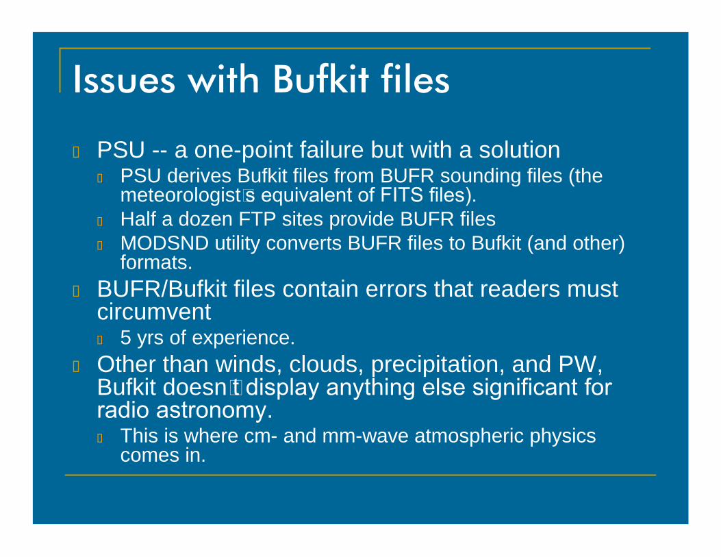
Issues with Bufkit files
PSU -- a one-point failure but with a solution PSU derives Bufkit files from BUFR sounding files (the
meteorologist’s equivalent of FITS files). Half a dozen FTP sites provide BUFR files MODSND utility converts BUFR files to Bufkit (and other)
formats. BUFR/Bufkit files contain errors that readers must
circumvent 5 yrs of experience.
Other than winds, clouds, precipitation, and PW, Bufkit doesn’t display anything else significant for radio astronomy. This is where cm- and mm-wave atmospheric physics
comes in.

References G. Brussaard and P.A. Watson, “Atmospheric Modelling and Millimetre Wave
Propagation,”, 1995, (New York: Chapman & Hall) B. Butler, "Precipitable Water Vapor at the VLA -- 1990 - 1998", 1998, NRAO MMA Memo
#237 (and references therein). L. Danese and R.B. Partridge, "Atmospheric Emission Models: Confrontation between
Observational Data and Predictions in the 2.5-300 GHz Frequency Range", 1989, AP.J.342, 604.
K.D. Froome and L. Essen, "The Velocity of Light and Radio Waves", 1969, (New York: Academic Press).
W.S. Smart, "Textbook on Spherical Astronomy", 1977, (New York: Cambridge Univ. Press).
H.J. Lehto, "High Sensitivity Searches for Short Time Scale Variability in Extragalactic Objects", 1989, Ph.D. Thesis, University of Virginia, Department of Astronomy, pp. 145-177.
H.J. Liebe, "An Updated model for millimeter wave propagation in moist air", 1985, Radio Science, 20, 1069
R.J. Maddalena "Refraction, Weather Station Components, and Other Details for Pointing the GBT", 1994, NRAO GBT Memo 112 (and references therein).
J. Meeus, "Astronomical Algorithms", 1990 (Richmond: Willman-Bell). K. Rohlfs and T.L. Wilson, "Tools of Radio Astronomy, 2nd edition", 1996, pp. 165-168. P.W. Rosenkranz, 1975, IEEE Trans, AP-23, 498. J.M. Rueger, "Electronic Distance Measurements", 1990 (New York: Springer Verlag). F.R. Schwab, D.E Hogg, and F.N. Owen, "Analysis of Radiosonde Data for the MMA
Site Survey and Comparison with Tipping Radiometer Data" (1989), from the IAU Symposium on "Radio Astronomical Seeing", pp 116-121.
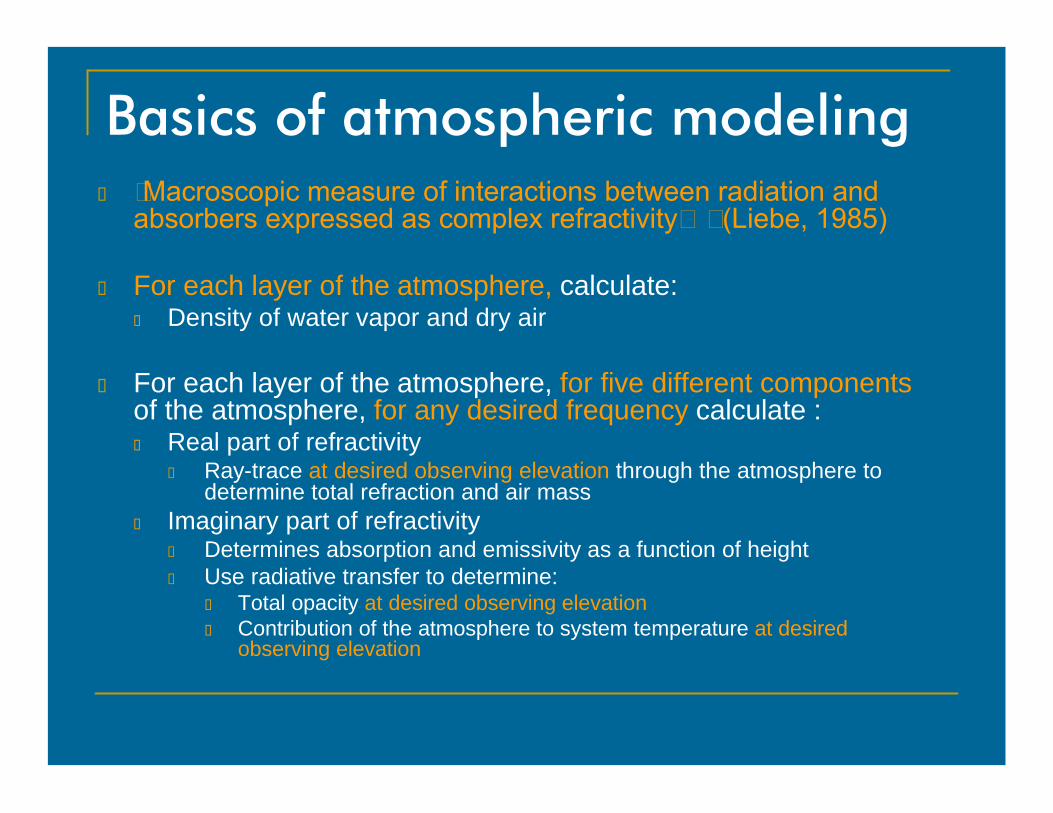
Basics of atmospheric modeling “Macroscopic measure of interactions between radiation and
absorbers expressed as complex refractivity…” (Liebe, 1985)
For each layer of the atmosphere, calculate: Density of water vapor and dry air
For each layer of the atmosphere, for five different componentsof the atmosphere, for any desired frequency calculate : Real part of refractivity
Ray-trace at desired observing elevation through the atmosphere to determine total refraction and air mass
Imaginary part of refractivity Determines absorption and emissivity as a function of height Use radiative transfer to determine:
Total opacity at desired observing elevation Contribution of the atmosphere to system temperature at desired
observing elevation

Basics of atmospheric modeling
So far, this is not new stuff. Has been done many times before with balloon data or using a ‘model’atmosphere. What is new? Uses recently-available forecasted weather data Updates automatically twelve times a day for every desired
frequency, elevation, time, site, and model (GFS, NAM, …). Automatically summarizes the results on the WWW in a
useful way for predicting conditions for radio astronomy Automates the generation of an archive Provides tools that anyone can use to mine the current and
archived forecasts in ways the WWW summaries do not. Applied to a sea-level, mid-Atlantic, 100-m telescope that
can observe up to 115 GHz and down to an elevation of 5º.

Refractivity at different heights Modeled as arising from five components of the atmosphere
Dry air continuum Non-resonant Debye spectrum of O2 below 100 GHz, pressure-induced
N2 attenuation > 100 GHz Water vapor rotational lines:
22.2, 67.8 & 120.0, 183.3 GHz, and higher Water vapor continuum from an unknown cause
“Excess Water Vapor Absorption” problem Oxygen spin rotation resonance line
Band of lines 51.5 – 67.9 GHz, single line at 118.8 GHz, and higher Modeled using Rosenkranz’s (1975) impact theory of overlapping lines
Hydrosols Mie approximation of Rayleigh scattering from suspended water
droplets with size < 50 μm

How it works….CFRLT P DP
30 km
…
920 m
880 m
κTotalκHydrosolsκO2κH2O LineκH2O_ContκDrynρDryρWaterh
Generate a table for every desired frequency, site, time

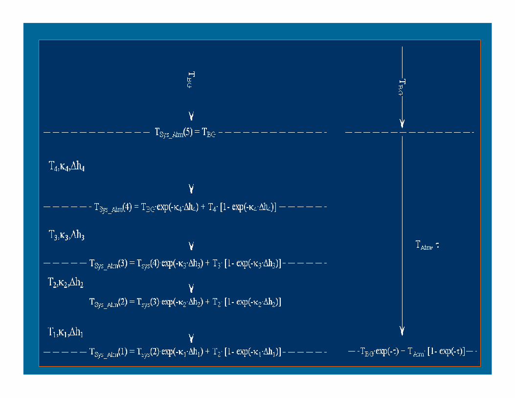
Basics of radiative transfer
H
0Total
H
0Total
Atm
AirMass)(Atm
AtmSys
dh),h(dh),h(AtmSys
AtmSys
H
0Total
iTotal
dh),h(
dh)h(T),h(T
)e1(T),0(T
)e1()h(Te)dhh(T),h(T
dh),h()(
),h(),h(
TotalTotal

Opacities from the various components
Dry Air Continuum

Opacities from the various components
Water Continuum
gfs3_c27_1190268000.buf

Opacities from the various components
Water Line
gfs3_c27_1190268000.buf

Opacities from the various components
Oxygen Line
gfs3_c27_1190268000.buf

Opacities from the various components
Hydrosols
gfs3_c27_1190268000.buf

Opacities from the various components
Total Opacity
gfs3_c27_1190268000.buf

Hydrosols – the big unknown Require water droplet density Not well forecasted Using the Schwab, Hogg, Owen (1989) model of
hydrosols Compromise technique Assumes a cloud is present in any layer of the atmosphere
where the humidity is 95% or greater. The thickness of the cloud layer determines the density 0.2 g/m3 for clouds thinner than 120 m 0.4 g/m3 for clouds thicker than 500 m, linearly-interpolated densities for clouds of intermediate
thickness And forget about it when it rains! No longer
droplets!!

Relative Effective System Temperatures: A way to judge what frequencies are most productive under various weather and observing conditions
Atmosphere hurts you twice Absorbs so your signal is weaker: TBG exp(-τ) Emits so your Tsys and noise go up:
Tsys = TRcvr + TSpill +TCMB exp(-τ)] + TAtm [1 – exp(-τ)] Signal-to-noise goes as:
TBG exp(-τ)/Tsys
Define Effective System Temperature (EST) as:
Proportional to the square root of the integration time needed to achieve a desired signal to noise
-Sys
-
-Atm
-CMBSpillRcvr
eT
e]e– [1TeTTT
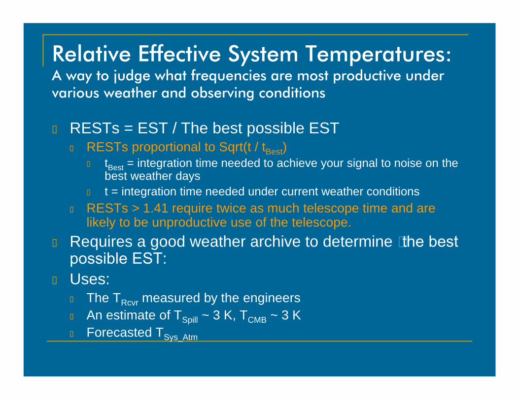
Relative Effective System Temperatures: A way to judge what frequencies are most productive under various weather and observing conditions
RESTs = EST / The best possible EST RESTs proportional to Sqrt(t / tBest)
tBest = integration time needed to achieve your signal to noise on the best weather days
t = integration time needed under current weather conditions RESTs > 1.41 require twice as much telescope time and are
likely to be unproductive use of the telescope. Requires a good weather archive to determine “the best
possible EST: Uses:
The TRcvr measured by the engineers An estimate of TSpill ~ 3 K, TCMB ~ 3 K Forecasted TSys_Atm

a = Earth radiusn(h) = index of refraction at height hn0 = index of refraction at surfaceρ(h) = air densityElevObs, ElevTrue = refracted and airless elevations
Basics of refraction and relative air mass
Elev Elev a n Elevdn h
n h a h n h a n ElevObs True ObsObs
n
0 2 2 2
02 2
1
0
cos( )( )
( ) ( ) ( ) cos ( )
AirMass Elev
h dh
h dh
aa h
nn h Elev
Obs
Obs
( )
( )
( )
( ) cos ( )
1
1
0
02
20

Also provide
Ground level values for Precipitable Water ∑ρWater(h) – good summary statistic Temperature and wind speeds (safety limits) Pressure, humidity, wind direction Fractional cloud cover = max[CFRL(h)] – for continuum
observers Comparison of various refraction models
Differential refraction and air mass Surface actuator displacement to take out atmospheric-
induced, weather-dependent astigmatism Summary forecasts from weather.com
Also archived NWS weather alerts.

Current modeling and limitations
Uses Liebe’s Microwave Propagation Model, with Danese & Partridge’s (1989) modifications plus some practical simplifications Although accurate up to 1000 MHz, current implementation <
230 GHz to save processing time Uses the Froome & Essen frequency-independent
approximation of refraction (to save processing time) Opacities < 5 GHz are too high for an unknown reason Cloud predictions (presence, thickness) are not very accurate Model for determining opacities from clouds (hydrosols) does
not match observations Schwab, Hogg, Owen model for water drop density and size may
not be accurate enough

Current modeling and limitations
Uses a ‘fuzzy’ cache of opacities to save processing at the expense of memory and accuracy
Fractional cloud cover does not consider whether a cloud is cold or warm (i.e. its importantance).
Must extrapolate real part of refractivity to 50 km (forecasts go to 30 km).
Assumes all absorption is below 30 km Total opacity estimate uses 1/sin(elev) instead of
ray-traced path TRcvr table, used for calculating RESTS, has a 1 or 2
GHZ resolution.

How accurate are ground-level values and a standard atmosphere?

How useful is the 86 GHz tipper?

How useful is the 86 GHz tipper?

How useful is the 86 GHz tipper?

How accurate are the forecasts?

How accurate are the forecasts?

How accurate are the forecasts?

How was our old DSS working?

Web Page Summaries
http://www.gb.nrao.edu/~rmaddale/Weather/index.html 3.5 and 7 day NAM and GFS forecasts. For each, provides::
Ground weather conditions Opacity and TAtm as a function of time and frequency Tsys and RESTs as functions of time, frequency, and elevation Refraction, differential refraction, comparison to other refraction
models
Weather.com forecasts NWS alerts Short summary of the modeling List of references

User Software: cleo forecasts
Type:
cleo forecasts
Or
cleo forecasts -help

User Software: cleo forecasts

User Software : forecastsCmdLine
To run, type: ~rmaddale/bin/forecastsCmdLine -help
cleo forecasts is a user-friendly GUI front end to forecastsCmdLine
Much more powerful and flexible than what the GUI allows
Generates text files only, no graphs cleo forecasts can graph files generated by a
previous run of forecastsCmdLine

User Software : forecastsCmdLine Fuzzy caching Reads Zipped archive files Writes processed data to time-tagged directories that contain a
log of user inputs and self documented files Extrapolation for upper atmosphere refraction Interpolation of missing data Table of TRcvr with 1 GHz resolution Accurate algorithms and approximations for Air mass and TAtm Lower accuracy but fast to calculate opacity estimates using the
models of H. Lehto Default is to use the best data (last forecasted for any time slot)
but there’s a super-user mode of time-offsetting

User Software : getForecastValues
To run, type: ~rmaddale/bin/getForecastValues –help
Fast way to retrieve opacities, TSys, RESTs, and TAtm for any frequency and any time after April 1, 2008
Returns results to standard output Uses a polynomial fit of these quantities Automatically produced and archived by the
system that generates the web pages
Weather Forecasting for Radio Astronomy
Part I: The Mechanics and Physics
Ronald J MaddalenaAugust 1, 2008


