Name: ___________________________________

Identifying and quantifying phytoplankton and zooplankton in

Oyster Pond, Falmouth MA

1. Get ready to identify and determine cell densities of plankton in Oyster Pond! These tiny

organisms span diverse evolutionary branches of life and reflect an enormous amount of

genetic, morphological and physiological complexity. There are guides available around the

room to help you identify the taxa you see. Communicate with your partner throughout the

exercise to ensure you are using a consistent identification scheme. Trade off using the

microscope to give your eyes a break.

a. For phytoplankton:

i. Grab a slide and cover slip – be careful, both are glass. Using a plastic

pipettor, add 1 drop of concentrated pond water onto the slide. Cover with

cover slip. Dab edges of cover slip with paper towel to soak up excess fluid.

b. For zooplankton:

i. Grab a petri dish. Using a plastic pipettor, add in 3 mL (3 full squirts) of the

net tow sample.

ii. Measure the total volume of filtrate using graduated cylinders. This will be

used to calculate the total amount of cells you count per liter of Oyster Pond

water (cells/L). Fill in below. Pour water back into bottles when done.

iii. Station 1 ____________, Station 2 ____________, Station 3_______________

2. Turn the compound light microscope or dissecting scope on. The main difference between

the two is the level of magnification. Light microscopes can typically magnify objects by

400-1000x, whereas dissecting scopes are more limited to 10-40X. Both scopes have eye

pieces and zoom lenses for combined magnification. We will use the light microscopes for

phytoplankton (size range: 2-200 µm), and dissecting scopes for zooplankton (size range:

200-2,000,000 µm).

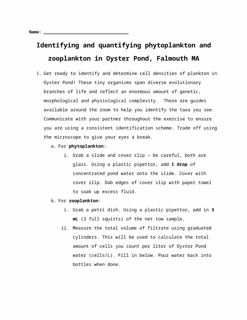
Figure 1. Light microscopes allow for up to 1,000-fold magnification and only require bright light and lenses. Electron microscopes such as the transmission electron microscopes (TEM) use a beam of electrons rather than light and can magnify up to one million-fold. Scanning electron microscopes (SEM) also utilize electrons but in contrast to TEM, allow for 3D imaging. (Alberts, B., Bray, D., Hopkin, K., Johnson, A., Lewis, J., Raff, M., Roberts K., Walter, P. Essential Cell Biology. New York: Garland Science, 2003.)

Figure 2. Light microscope components.

Figure 3. Dissection scope components, from cmore.soest.hawaii.edu/education.htm

3. Both microscopes have lamps that can be adjusted for brightness, and eye pieces that can be

moved to accommodate each user. Adjust distance between eye pieces until you can

comfortably see only one circle.

4. To focus the scopes, start out on the least magnification. On the light microscope, this would

be the weakest objective: 4X. On the dissection scope, this will be 1X. Carefully increase

magnification by turning the focusing knob clockwise until you see a sharp image. Go slow!

Too much force on the light microscope may cause the objective to crash into the slide.

5. Look through the sample to get an idea of which taxonomic groups are present and

identifiable. Make a table in your notebook to and keep track of the major groups. Example

tables might look like the ones below. You may very well find other/different groups

present in your samples!! During your initial survey to observe what we collected, feel free

to use the weak objectives. Count using the stronger objectives (3X [dissecting] or 40X

[light]).

Dissecting St. 1 St. 1 St. 1 St. 2 St. 2 St. 2 St. 3 St. 3 St. 3

Copepod

Nauplius

Water flea

(Cladocerans)

Light St. 1 St. 2 St. 3

Green algae

Dinoflagellate

Haptophyte

Diatom

Start counting! Take your time identifying. Make a table on a blank sheet of paper, and use a

new table for each station. The most important point to remember is to be consistent with

you naming convention. Take your time and be specific as you can be given the resources

available. If group A identifies a diatom down to the genus and calls it Chaetoceros , and

group B calls it “Box-like diatom with spikes”, we can still track its abundance pattern

across sites. Sketch or photograph each major taxonomic group you are counting (diatom,

dinoflagellate, copepod, etc.) so you can compare with others later on. If you ID an organism

and you feel confident about it, sketch it on the white board to share with others.

If you cannot count the zooplankton due to too much movement, use the nontoxic Lugol’s

preservative to fix (kill) cells. You only need to add 5 drops to your 3 mL petri dish. Be

sure to discard this solution in the “Lugol’s waste” container when you are finished, not

back into the glass jar. This solution stains clothing – be careful.

Be sure to only count a given taxon either under the light or dissecting scope, not both.

For example, if you see rotifers in both the light microscope and dissecting scope, choose

the more appropriate view to count with. (Since rotifers are quite large, count them under

the dissecting scope. Phytoplankton colonies are easier to identify under the light

microscope).

a. Phytoplankton groups should count the full slide. Once complete, go on to the next

station. Rinse the slide with tap water in between. Be especially careful with the

glass cover slip.

b. Zooplankton groups should count the full petri dish. Once complete, repeat with

the same station sample three more times for replication. Then go on to the next

station and repeat. Dump pond water back into original bottle if no Lugol’s was

added. If it was, put in the “Lugol’s waste” bottle. Take at least one picture with the

SnapZoom phone holder.

6. Once finished with either phytoplankton or zooplankton counts, switch over to opposite

group. Perform counts similarly in a new table, labeled for each station.

7. Calculate cells per liter (cells/L) for each major group of organisms you identified (combine

into diatoms, dinoflagellates, copepods, etc.) Assume a boat speed of 0.5 knots, which

equals ~ 0.25 meter/second.

Using distance (d) [meters] = velocity (v) [meters/seconds] * time (t) [seconds],

what is the distance we traveled for each of the stations? (Use a calculator for

precision, keep units consistent).

Station 1 ____________, Station 2 _____________, Station 3_________________

8. How much water was filtered using the volume of a cylinder: rπ 2*h (in this case, height (h)

= distance (d) calculated above, and r = 0.25 meters)? Your units should be in m3. Convert

this value to liters using the following conversion: 1m3 = 1,000 liters (L).

Station 1 ____________, Station 2 _____________, Station 3_________________

9. Since you didn’t count the full water sample, you will need to extrapolate your results. Using

the following formula, calculate how many cells you would have counted in the original

volume based on your counts in 0.003 L (3 mL, for zooplankton) or 0.0001 L (~1 drop = 100

µL, for phytoplankton). Use Microsoft Excel if you are comfortable doing so, but you may

also easily calculate by hand and include the corrected counts in a new table.

counts youmeasured for eachgroup0.003L∨0.0001L(subsample) =

xvolume of net tow sample( part 1)

10. Almost done! Now determine the density of cells in Oyster Pond water at each station.

Include this in a new table, for each major group:

number of cells ( part 9)Oyster Pond water volume sampled ( part 8) = cells/L

11. When done, turn off microscopes. Rinse out petri dishes and/or slides with tap water.

Next we will graph our phytoplankton and zooplankton data in R. Bar graphs are useful for

observing trends across locations, time, or treatments. This exercise has been adapted from

David Lillis on theanalysisfactor.com. There are many, many more resources available

online if you are interested in further exploring visualization tools in R, including

scatterplots, pie charts, bubble plots, ordination plots, and heatmaps to name a few.

1. Open a blank Microsoft Excel template and type in your counts table for the zooplankton.

Your rows should be different taxonomic groups, columns are different stations and

replicates. Save as a comma separated value (.csv) file to your desktop for easy importing

into R.

2. In RStudio, set your working directory to your desktop under the “Session” tab in the tool

bar.

3. Read in text file for phytoplankton and zooplankton separately. Let’s start with

phytoplankton.

zoo_counts<-read.csv(file.choose())

4. Now your data frame is a combination of words (taxonomic groups) and numbers (counts).

To generate graphs, we want to remove the taxonomic groups from the data frame and

instead use them as row identifiers. Set the row names equal to the taxa column and then

delete the first column.

rownames(zoo_counts)<-zoo_counts$X

zoo_counts<-zoo_counts[,-1]

head(zoo_counts)

5. Take a look at the bar graph:

barplot(as.matrix(zoo_counts))

6. Let’s add color, a title, and a y-axis label, and separate out the groups.

colors <- c("brown", "red", "green")

Put down as many colors as you have groups. For instance, if you counted diatoms,

dinoflagellates, and volvox, you should only list 3 colors.

barplot(as.matrix(zoo_counts), main="Oyster Pond Plankton", ylab

= "Cells/L", beside=TRUE, col=colors)

When beside is set to TRUE, your bar graphs will no longer be stacked. 7. Now we need to add a legend. We will add on to our previous line using “+”. Use the up key

in R to bring back your previous command.

barplot(as.matrix(zoo_counts), main="Oyster Pond Plankton",

ylab = "Cells/L", beside=TRUE, col=colors) + legend("topleft", c("Diatom","Dinoflagellate","Volvox"), bty="n", fill=colors)

8. Repeat for your phytoplankton table and generate a second bar graph.

Next we will determine whether the differences in zooplankton counts across stations is

statistically significant. This is only possible for data with replicates, so we can only perform this

test for the zooplankton.

1. We need the data in a slightly different format. Whereas before our columns were

sites and rows were counts, we now need the inverse. Invert your table using the

transpose function available in the “data.table” R package.

install.packages("data.table")

library(data.table)

countsT<-transpose(zoo_counts)

colnames(countsT) <- rownames(zoo_counts)

rownames(countsT) <- colnames(zoo_counts)

2. Last few steps: we need to bring back the sites as their own column instead of a row

name. Recall that we removed it initially to make the bar plot. R doesn’t allow

multiple columns to have the same name. Now that the sites are rows, we can give

all replicates identical names (St. 1, St. 2, St. 3). This will be necessary for the stats

test.

countsT$site<-rowname(countsT)

head(countsT)

countsT$site<-rep(c("St.1","St.2","St.3"),3)

head(counts)

Your table should look something like this:

3. For the demonstration, I followed the quick audio guide available on Ed Boone’s

Youtube channel. Run an analysis of variance test (ANOVA) on each group

separately. Starting with the first group (e.g., dinoflagellates), let’s see if there are

any differences in the average cells/L across sites.

dinoflagellate.aov<-aov(countsT$dinoflagellate ~

countsT$site)

summary(dinoflagellate.aov)

You should see a summary table with ANOVA parameters listed, including the test comparison you

ran, degrees of freedom, sum of squares, mean squares, F value and p value. Generally, a p value of

less than 0.05 (p < 0.05) is considered significant.

4. If a difference exists, where are they? We can further examine using the Tukey

multiple comparison test.

TukeyHSD(dinoflagellate.aov)

Significant differences in diatom counts between sites will have a p value of less than 0.05 listed in

that comparison row. In my example below, sites 1 vs. 2, and sites 2 vs. 3 show significant

differences in dinoflagellate abundance.

1. Do you think your cell counts accurately reflect cell densities in Oyster Pond? Why

or why not?

2. Are your counts similar to those obtained by other groups? Why or why not? Which

groups were easiest to identify and which the most challenging? What would you

recommend for future researchers aiming to cross compare cell counts from Oyster

Pond?

3. What other some other approaches that might be appropriate for assessing

diversity and abundance of marine plankton, apart from light microscopy?

4. Based on your data, which taxonomic groups are most successful in Oyster Pond and

why? Do you think their morphology is linked to their ecological success? What

physiological adaptations are used to survive in this environment?

5. Did you observe any patterns in plankton abundance across pond sites?

6. What types of physical or chemical stressors are Oyster Pond plankton frequently

faced with and how do you think they respond? How might these freshwater

responses differ from their marine counterparts?