Week 1: Newton s Laws

Contents

Introduction and some Mathematics Elementary Mechanics and Newton's Laws

o Dynamicso Coordinateso Newton's Lawso Forceso Simple Motion in One Dimension.o Motion in Two Dimensions.o Circular Motiono Friction

Work and Energyo The Work-Kinetic Energy Theoremo Conservative Forces: Potential Energyo Conservation of Mechanical Energyo Powero Equilibrium

Systems of Particles, Momentum and Collisionso Systems of Particleso Momentumo Impulseo Center of Mass Reference Frameo Collisions

Staticso Conditions for Static Equilibrium

Fluidso General Fluid Properties.o Pressureo Densityo Compressibilityo Viscosity and fluid flowo Static Fluidso Pascal's Principle and Hydraulicso Fluid Flowo The Human Circulatory System

I Semester

Based on the Physics course of Duke University https://www.phy.duke.edu/

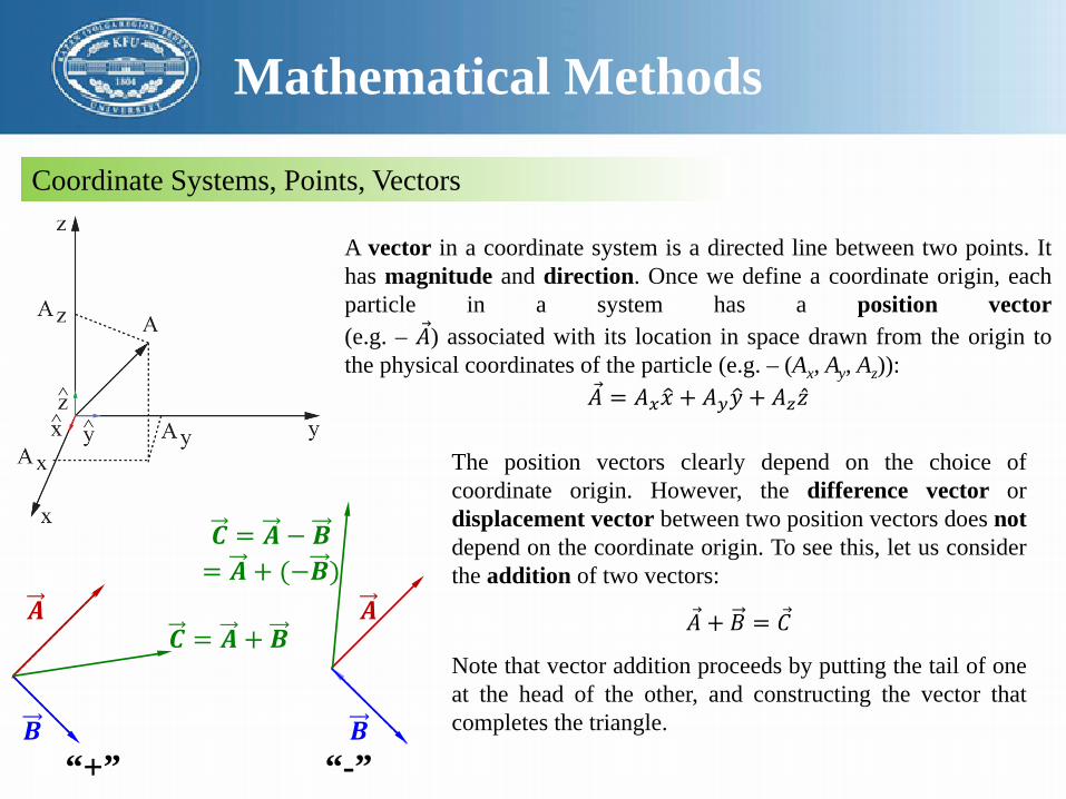
A vector in a coordinate system is a directed line between two points. Ithas magnitude and direction. Once we define a coordinate origin, eachparticle in a system has a position vector(e.g. – 𝐴𝐴) associated with its location in space drawn from the origin tothe physical coordinates of the particle (e.g. – (Ax, Ay, Az)):

𝐴𝐴 = 𝐴𝐴𝑥𝑥 �𝑥𝑥 + 𝐴𝐴𝑦𝑦 �𝑦𝑦 + 𝐴𝐴𝑧𝑧�̂�𝑧

𝑨𝑨

𝑩𝑩

𝑨𝑨

𝑩𝑩“+” “-”

Mathematical Methods

Coordinate Systems, Points, Vectors

The position vectors clearly depend on the choice ofcoordinate origin. However, the difference vector ordisplacement vector between two position vectors does notdepend on the coordinate origin. To see this, let us considerthe addition of two vectors:

𝐴𝐴 + 𝐵𝐵 = 𝐶𝐶

Note that vector addition proceeds by putting the tail of oneat the head of the other, and constructing the vector thatcompletes the triangle.

𝑪𝑪 = 𝑨𝑨 + 𝑩𝑩

𝑪𝑪 = 𝑨𝑨 − 𝑩𝑩= 𝑨𝑨 + (−𝑩𝑩)

Vector

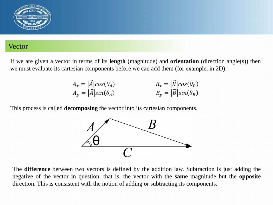
If we are given a vector in terms of its length (magnitude) and orientation (direction angle(s)) thenwe must evaluate its cartesian components before we can add them (for example, in 2D):

𝐴𝐴𝑥𝑥 = 𝐴𝐴 𝑐𝑐𝑐𝑐𝑐𝑐 𝜃𝜃𝐴𝐴 𝐵𝐵𝑥𝑥 = 𝐵𝐵 𝑐𝑐𝑐𝑐𝑐𝑐 𝜃𝜃𝐵𝐵𝐴𝐴𝑦𝑦 = 𝐴𝐴 𝑐𝑐𝑠𝑠𝑠𝑠 𝜃𝜃𝐴𝐴 𝐵𝐵𝑦𝑦 = 𝐵𝐵 𝑐𝑐𝑠𝑠𝑠𝑠 𝜃𝜃𝐵𝐵

This process is called decomposing the vector into its cartesian components.

The difference between two vectors is defined by the addition law. Subtraction is just adding thenegative of the vector in question, that is, the vector with the same magnitude but the oppositedirection. This is consistent with the notion of adding or subtracting its components.

Scalar

When we reconstruct a vector from its components, we are just using the law of vector addition itself,by scaling some special vectors called unit vectors and then adding them. Unit vectors are (typicallyperpendicular) vectors that define the essential directions and orientations of a coordinate system andhave unit length. Scaling them involves multiplying these unit vectors by a number that represents themagnitude of the vector component. This scaling number has no direction and is called a scalar.

𝐵𝐵 = 𝐶𝐶𝐴𝐴where C is a scalar (number) and 𝐴𝐴 is a vector. In this case, 𝐴𝐴 || 𝐵𝐵 (𝐴𝐴 is parallel to 𝐵𝐵).

𝑩𝑩

𝑨𝑨 𝑨𝑨 𝑨𝑨 𝑨𝑨 𝑨𝑨

Let’s define products that multiply two vectors together

The first product creates a scalar (ordinary number with magnitude but no direction) out of twovectors and is therefore called a scalar product or (because of the multiplication symbol chosen) adot product.

𝐴𝐴 = + 𝐴𝐴 � 𝐴𝐴

𝐴𝐴 � 𝐵𝐵 = 𝐴𝐴𝑥𝑥 ∗ 𝐵𝐵𝑥𝑥 + 𝐴𝐴𝑦𝑦 ∗ 𝐵𝐵𝑦𝑦 … = 𝐴𝐴 𝐵𝐵 cos(𝜃𝜃𝐴𝐴𝐵𝐵)

A scalar product is the length of one vector (either one, say |𝐴𝐴|) times the component of the other vector (|𝐵𝐵| 𝑐𝑐𝑐𝑐𝑐𝑐 𝜃𝜃𝐴𝐴𝐵𝐵 ) that points in the same direction as the vector 𝐴𝐴. This product is symmetric and commutative (𝐴𝐴 and 𝐵𝐵 can appear in either order or role).

𝑩𝑩

𝑨𝑨

𝜽𝜽

𝐴𝐴 cos(𝜃𝜃)

A vector productThe other product multiplies two vectors in a way that creates a third vector. It is called a vector product or (because of the multiplication symbol chosen) a cross product.

𝐴𝐴 × 𝐵𝐵 = 𝐴𝐴𝑥𝑥 ∗ 𝐵𝐵𝑦𝑦 − 𝐴𝐴𝑦𝑦 ∗ 𝐵𝐵𝑥𝑥 �̂�𝑧 + 𝐴𝐴𝑦𝑦 ∗ 𝐵𝐵𝑧𝑧 − 𝐴𝐴𝑧𝑧 ∗ 𝐵𝐵𝑦𝑦 �𝑥𝑥 + 𝐴𝐴𝑧𝑧 ∗ 𝐵𝐵𝑥𝑥 − 𝐴𝐴𝑥𝑥 ∗ 𝐵𝐵𝑧𝑧 �𝑦𝑦

𝐴𝐴 × 𝐵𝐵 = 𝐴𝐴 𝐵𝐵 sin(𝜃𝜃𝐴𝐴𝐵𝐵)

𝐴𝐴 × 𝐵𝐵 = −𝐵𝐵 × 𝐴𝐴

Let’s define the direction of the cross product using the right hand rule:

Let the fingers of your right hand lie along the direction of the first vector in across product (say 𝐴𝐴 below). Let them curl naturally through the small angle(observe that there are two, one of which is larger than π and one of which isless than π) into the direction of 𝐵𝐵 . The erect thumb of your right hand thenpoints in the general direction of the cross product vector – it at leastindicates which of the two perpendicular lines should be used as a direction,unless your thumb and fingers are all double jointed or your bones aremissing or you used your left-handed right hand or something.

𝑩𝑩𝑨𝑨𝜽𝜽

𝑨𝑨 × 𝑩𝑩

𝑩𝑩 × 𝑨𝑨 = −𝑨𝑨 × 𝑩𝑩

Lecture 1. Newton’s Laws

Coordinates

Physics is the study of dynamics. Dynamics is the description of the actual forces of nature that, webelieve, underlie the causal structure of the Universe and are responsible for its evolution in time. Weare about to embark upon the intensive study of a simple description of nature that introduces theconcept of a force, due to Isaac Newton. A force is considered to be the causal agent that producesthe effect of acceleration in any massive object, altering its dynamic state of motion.

a) meters – the SI units of lengthb) seconds – the SI units of timec) kilograms – the SI units of mass

Coordinatized visualization of the motion of a particleof mass m along a trajectory x⃗(t). Note that in a shorttime Δt the particle’s position changes from x⃗(t) tox⃗(t+Δt) .

x⃗(t)=x(t) �𝑥𝑥 + 𝑦𝑦(𝑡𝑡) �𝑦𝑦


Velocity

The average velocity of the particle is by definition the vector change in its position ∆x⃗ in some time Δtdivided by that time:

�⃗�𝑣𝑎𝑎𝑎𝑎 =∆�⃗�𝑥∆𝑡𝑡

Sometimes average velocity is useful, but often, even usually, it is not. It can be a rather poor measure forhow fast a particle is actually moving at any given time, especially if averaged over times that are longenough for interesting changes in the motion to occur.

The instantaneous velocity vector is the time-derivative of the position vector:

�⃗�𝑣 𝑡𝑡 = lim∆𝑡𝑡→0

�⃗�𝑥 𝑡𝑡 + ∆𝑡𝑡 − �⃗�𝑥(𝑡𝑡)∆𝑡𝑡

= lim∆𝑡𝑡→0

∆�⃗�𝑥∆𝑡𝑡

=𝑑𝑑�⃗�𝑥𝑑𝑑𝑡𝑡

Speed is defined to be the magnitude of the velocity vector:𝑣𝑣 𝑡𝑡 = �⃗�𝑣(𝑡𝑡)


Acceleration

To see how the velocity changes in time, we will need to consider the acceleration of a particle, or therate at which the velocity changes. As before, we can easily define an average acceleration over apossibly long time interval Δt as:

�⃗�𝑎𝑎𝑎𝑎𝑎 =�⃗�𝑣 𝑡𝑡 + ∆𝑡𝑡 − �⃗�𝑣(𝑡𝑡)

∆𝑡𝑡=𝑑𝑑�⃗�𝑣𝑑𝑑𝑡𝑡

The acceleration that really matters is (again) the limit of the average over very short times; the timederivative of the velocity. This limit is thus defined to be the instantaneous acceleration:

�⃗�𝑎 𝑡𝑡 = lim∆𝑡𝑡→0

∆�⃗�𝑣∆𝑡𝑡

=𝑑𝑑�⃗�𝑣𝑑𝑑𝑡𝑡

=𝑑𝑑2�⃗�𝑥𝑑𝑑𝑡𝑡2


Newton’s Laws

a) Law of Inertia: Objects at rest or in uniform motion (at a constant velocity) in an inertial reference frame remain so unless acted upon by an unbalanced (net, total) force. We can write this algebraically as:

�⃗�𝐹 = ∑𝑖𝑖 �⃗�𝐹𝑖𝑖 = 0 = 𝑚𝑚�⃗�𝑎 = 𝑚𝑚𝑑𝑑𝑎𝑎𝑑𝑑𝑡𝑡⇒ �⃗�𝑣 = 𝑐𝑐𝑐𝑐𝑠𝑠𝑐𝑐𝑡𝑡𝑎𝑎𝑠𝑠𝑡𝑡 𝑣𝑣𝑣𝑣𝑐𝑐𝑡𝑡𝑐𝑐𝑣𝑣

b) Law of Dynamics: The total force applied to an object is directly proportional to its acceleration in an inertial reference frame. The constant of proportionality is called the mass of the object. We write this algebraically as:

�⃗�𝐹 = �𝑖𝑖

�⃗�𝐹𝑖𝑖 = 𝑚𝑚�⃗�𝑎 =𝑑𝑑(𝑚𝑚�⃗�𝑣)𝑑𝑑𝑡𝑡

=𝑑𝑑�⃗�𝑝𝑑𝑑𝑡𝑡

where we introduce the momentum of a particle, �⃗�𝑝 = 𝑚𝑚�⃗�𝑣.c) Law of Reaction: If object A exerts a force �⃗�𝐹𝐴𝐴𝐵𝐵 on object B along a line connecting the two objects, then object B

exerts an equal and opposite reaction force of �⃗�𝐹𝐴𝐴𝐵𝐵 = −�⃗�𝐹𝐵𝐵𝐴𝐴 on object A. We write this algebraically as:

�⃗�𝐹𝑖𝑖𝑗𝑗 = −�⃗�𝐹𝑗𝑗𝑖𝑖 𝑐𝑐𝑣𝑣 �𝑖𝑖,𝑗𝑗

�⃗�𝐹𝑖𝑖𝑗𝑗 = 0

where i and j are arbitrary particle labels. The latter form will be useful to us later; it means that the sum of all internal forces between particles in any closed system of particles cancels!


Forces

Classical dynamics at this level, in a nutshell, is very simple. Find the total force on an object. UseNewton’s second law to obtain its acceleration (as a differential equation of motion). Solve the equationof motion by direct integration or otherwise for the position and velocity.

The next most important problem is: how do we evaluate the total force?

There are fundamental forces – elementary forces that we call “laws of nature” because the forces themselves aren’t caused by some other force, they are themselves the actual causes of dynamical action in the visible Universe.

The Forces of Nature (strongest to weakest):

a) Strong Nuclear (bound together the quarks, protons and neutrons)

b) Electromagnetic (combines the positive nucleus with electrons)

c) Weak Nuclear (acts at very short range. This force can cause e.g. neutrons to give off an electron and turn into a proton)

d) Gravity


Force Rulesa) Gravity (near the surface of the earth):

𝐹𝐹𝑔𝑔 = 𝑚𝑚𝑚𝑚, 𝑚𝑚 ≈ 9,81 𝑚𝑚𝑚𝑚𝑡𝑡𝑚𝑚𝑚𝑚𝑠𝑠𝑚𝑚𝑠𝑠𝑠𝑠𝑠𝑠𝑑𝑑2

≈ 10 𝑚𝑚𝑚𝑚𝑡𝑡𝑚𝑚𝑚𝑚𝑠𝑠𝑚𝑚𝑠𝑠𝑠𝑠𝑠𝑠𝑑𝑑2

b) The Spring (Hooke’s Law) in one dimension:𝐹𝐹𝑥𝑥 = −𝑘𝑘∆𝑥𝑥

c) The Normal Force: 𝐹𝐹⊥ = 𝑁𝑁

d) Tension in an Acme (massless, unstretchable, unbreakable) string: 𝐹𝐹𝑆𝑆 = 𝑇𝑇

e) Static Friction:𝑓𝑓𝑆𝑆 ≤ 𝜇𝜇𝑠𝑠𝑁𝑁

f) Kinetic Friction:𝑓𝑓𝑘𝑘 = 𝜇𝜇𝑘𝑘𝑁𝑁

g) Fluid Forces, Pressure: A fluid in contact with a solid surface (or anything else) in general exerts a force on that surface that is related to the pressure of the fluid:

𝐹𝐹𝑃𝑃 = 𝑃𝑃𝐴𝐴h) Drag Forces:

𝐹𝐹𝑑𝑑 = −𝑏𝑏𝑣𝑣𝑠𝑠


Force Balance – Static Equilibrium

If all of the forces acting on an object balance:

�⃗�𝐹𝑡𝑡𝑠𝑠𝑡𝑡 = �𝑖𝑖

�⃗�𝐹𝑖𝑖 = 𝑚𝑚�⃗�𝑎 = 0

Example: Spring and Mass in Static Force Equilibrium

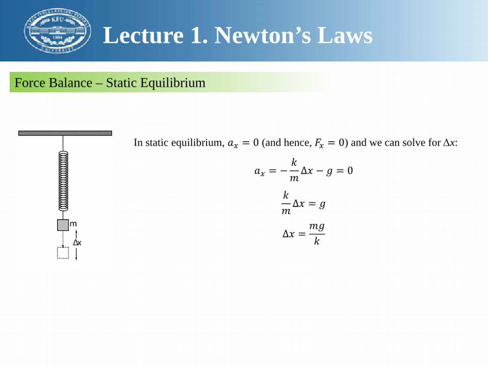
Suppose we have a mass m hanging on a spring with spring constant k such that the spring is stretched out some distance Δx from its unstretched length.

A mass m hangs on a spring with spring constant k. We would like to compute the amount Δxby which the string is stretched when the mass is at rest in static force equilibrium.

�𝐹𝐹𝑥𝑥 = −𝑘𝑘 𝑥𝑥 − 𝑥𝑥0 − 𝑚𝑚𝑚𝑚 = 𝑚𝑚𝑎𝑎𝑥𝑥

or (with Δx = x − x0, so that Δx is negative as shown)

𝑎𝑎𝑥𝑥 = −𝑘𝑘𝑚𝑚∆𝑥𝑥 − 𝑚𝑚


Force Balance – Static Equilibrium

In static equilibrium, 𝑎𝑎𝑥𝑥 = 0 (and hence, 𝐹𝐹𝑥𝑥 = 0) and we can solve for Δx:

𝑎𝑎𝑥𝑥 = −𝑘𝑘𝑚𝑚∆𝑥𝑥 − 𝑚𝑚 = 0

𝑘𝑘𝑚𝑚∆𝑥𝑥 = 𝑚𝑚

∆𝑥𝑥 =𝑚𝑚𝑚𝑚𝑘𝑘


Simple Motion in One Dimension

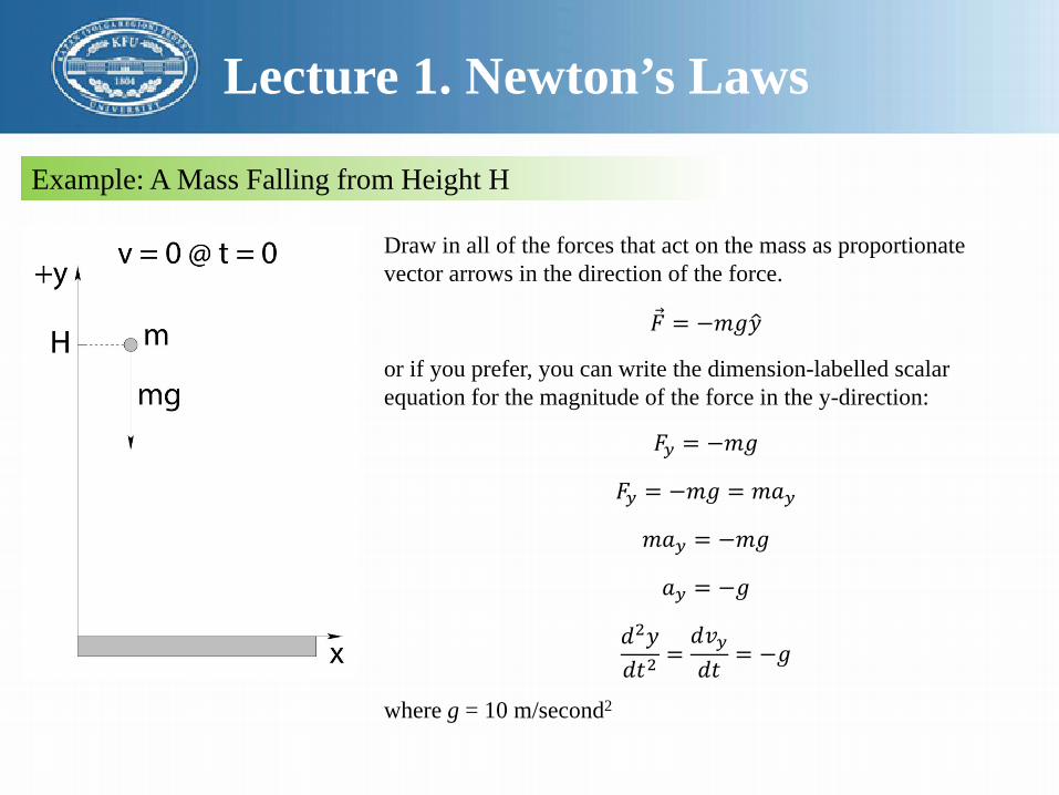
A mass m at rest is dropped from a height H above the ground at time t = 0; what happens to the mass as a function of time?

1. You must select a coordinate system to use to describe what happens.

2. You must write Newton’s Second Law in the coordinate system for all masses, being sure to include all forces or force rules that contribute to its motion.

3. You must solve Newton’s Second Law to find the accelerations of all the masses (equations called the equations of motion of the system).

4. You must solve the equations of motion to find the trajectories of the masses, their positions as a function of time, as well as their velocities as a function of time if desired.

5. Finally, armed with these trajectories, you must answer all the questions the problem poses using algebra and reason


Example: A Mass Falling from Height H

Draw in all of the forces that act on the mass as proportionate vector arrows in the direction of the force.

�⃗�𝐹 = −𝑚𝑚𝑚𝑚�𝑦𝑦

or if you prefer, you can write the dimension-labelled scalar equation for the magnitude of the force in the y-direction:

𝐹𝐹𝑦𝑦 = −𝑚𝑚𝑚𝑚

𝐹𝐹𝑦𝑦 = −𝑚𝑚𝑚𝑚 = 𝑚𝑚𝑎𝑎𝑦𝑦

𝑚𝑚𝑎𝑎𝑦𝑦 = −𝑚𝑚𝑚𝑚

𝑎𝑎𝑦𝑦 = −𝑚𝑚

𝑑𝑑2𝑦𝑦𝑑𝑑𝑡𝑡2

=𝑑𝑑𝑣𝑣𝑦𝑦𝑑𝑑𝑡𝑡

= −𝑚𝑚

where g = 10 m/second2


Example: A Mass Falling from Height H The last line (the algebraic expression for the acceleration) is called the equation of motion for the system

𝑑𝑑𝑎𝑎𝑦𝑦𝑑𝑑𝑡𝑡

= −𝑚𝑚 Next, multiply both sides by dt to get:

𝑑𝑑𝑣𝑣𝑦𝑦 = −𝑚𝑚𝑑𝑑𝑡𝑡 Then integrate both sides:

∫𝑑𝑑𝑣𝑣𝑦𝑦 = −∫𝑚𝑚𝑑𝑑𝑡𝑡 doing the indefinite integrals to get:

𝑣𝑣𝑦𝑦 𝑡𝑡 = −𝑚𝑚 � 𝑡𝑡 + 𝐶𝐶

The final C is the constant of integration of the indefinite integrals. We have to evaluate it using thegiven (usually initial) conditions. In this case we know that:

𝑣𝑣𝑦𝑦 0 = −𝑚𝑚 � 0 + 𝐶𝐶 = 𝐶𝐶 = 0

Thus:

𝑣𝑣𝑦𝑦 𝑡𝑡 = −𝑚𝑚𝑡𝑡

We now know the velocity of the dropped ball as a function of time!


Example: A Mass Falling from Height H However, the solution to the dynamical problem is the trajectory function, y(t). To find it, we repeat the same process, but now use the definition for vy in terms of y:

𝑑𝑑𝑦𝑦𝑑𝑑𝑡𝑡

= 𝑣𝑣𝑦𝑦 𝑡𝑡 = −𝑚𝑚𝑡𝑡 Multiply both sides by dt to get:

𝑑𝑑𝑦𝑦 = −𝑚𝑚𝑡𝑡 𝑑𝑑𝑡𝑡 Next, integrate both sides:

∫𝑑𝑑𝑦𝑦 = −∫𝑚𝑚𝑡𝑡 𝑑𝑑𝑡𝑡 to get:

𝑦𝑦 𝑡𝑡 = −12𝑚𝑚𝑡𝑡2 + 𝐷𝐷

The final D is again the constant of integration of the indefinite integrals. We again have to evaluate it using the given(initial) conditions in the problem. In this case we know that:

𝑦𝑦 0 = −12𝑚𝑚02 + 𝐷𝐷 = 𝐷𝐷 = 𝐻𝐻

because we dropped it from an initial height 𝑦𝑦 0 = 𝐻𝐻. Thus:

𝑦𝑦 𝑡𝑡 = −12𝑚𝑚𝑡𝑡2 + 𝐻𝐻

and we know everything there is to know about the motion!


Example: A Mass Falling from Height H Finally, we have to answer any questions that the problem might ask! Here are a couple of common questions you can now answer using the solutions you just obtained:

a) How long will it take for the ball to reach the ground?

b) How fast is it going when it reaches the ground?

To answer the first one, we use a bit of algebra. “The ground” is (recall) y = 0 and it will reach there at some specifictime (the time we want to solve for) tg.

We write the condition that it is at the ground at time tg :

𝑦𝑦 𝑡𝑡𝑔𝑔 = −12𝑚𝑚𝑡𝑡2 + 𝐻𝐻 = 0

If we rearrange this and solve for tg we get:

𝑡𝑡𝑔𝑔 = ±2𝐻𝐻𝑚𝑚


Example: A Mass Falling from Height H To find the speed at which it hits the ground, one can just take our correct (future) time and plug it into vy! That is:

𝑣𝑣𝑔𝑔 = 𝑣𝑣𝑦𝑦 𝑡𝑡𝑔𝑔 = −𝑚𝑚𝑡𝑡𝑔𝑔 = −𝑚𝑚2𝐻𝐻𝑚𝑚

= − 2𝑚𝑚𝐻𝐻

Note well that it is going down (in the negative y direction) when it hits the ground.


Example: A Constant Force in One DimensionA car of mass m is travelling at a constant speed v0 as it enters a long, nearly straight merge lane. Adistance d from the entrance, the driver presses the accelerator and the engine exerts a constant force ofmagnitude F on the car.

a) How long does it take the car to reach a final velocity vf > v0?

b) How far (from the entrance) does it travel in that time?


Example: A Constant Force in One DimensionWe will write Newton’s Second Law and solve for the acceleration (obtaining an equation of motion). Then we willintegrate twice to find first vx(t) and then x(t).

𝐹𝐹 = 𝑚𝑚𝑎𝑎𝑥𝑥

𝑎𝑎𝑥𝑥 = 𝐹𝐹𝑚𝑚

= 𝑎𝑎0 (a constant)

𝑑𝑑𝑣𝑣𝑥𝑥𝑑𝑑𝑡𝑡

= 𝑎𝑎0

Next, multiply through by dt and integrate both sides:

𝑣𝑣𝑥𝑥 𝑡𝑡 = �𝑑𝑑𝑣𝑣𝑥𝑥 = �𝑎𝑎0𝑑𝑑𝑡𝑡 = 𝑎𝑎0𝑡𝑡 + 𝑉𝑉 =𝐹𝐹𝑚𝑚𝑡𝑡 + 𝑉𝑉

V is a constant of integration that we will evaluate below.

Note that if 𝑎𝑎0 = 𝐹𝐹/𝑚𝑚 was not a constant (say that F(t) is a function of time) then we would have to do the integral:

𝑣𝑣𝑥𝑥 𝑡𝑡 = �𝐹𝐹(𝑡𝑡)𝑚𝑚

𝑑𝑑𝑡𝑡 =1𝑚𝑚�𝐹𝐹 𝑡𝑡 𝑑𝑑𝑡𝑡 =? ? ?


Example: A Constant Force in One Dimension

At time t = 0, the velocity of the car in the x-direction is v0, so V = v0 and:

𝑣𝑣𝑥𝑥 𝑡𝑡 = 𝑎𝑎0𝑡𝑡 + 𝑣𝑣0 =𝑑𝑑𝑥𝑥𝑑𝑑𝑡𝑡

We multiply this equation by dt on both sides, integrate, and get:

𝑥𝑥 𝑡𝑡 = �𝑑𝑑𝑥𝑥 = �(𝑎𝑎0𝑡𝑡 + 𝑣𝑣0)𝑑𝑑𝑡𝑡 =12𝑎𝑎0𝑡𝑡2 + 𝑣𝑣0𝑡𝑡 + 𝑥𝑥0

where x0 is the constant of integration. We note that at time t = 0, x(0) = d, so x0 = d. Thus:

𝑥𝑥 𝑡𝑡 =12𝑎𝑎0𝑡𝑡2 + 𝑣𝑣0𝑡𝑡 + 𝑑𝑑

𝑣𝑣𝑥𝑥 𝑡𝑡 = 𝑎𝑎0𝑡𝑡 + 𝑣𝑣0

𝑥𝑥 𝑡𝑡 =12𝑎𝑎0𝑡𝑡2 + 𝑣𝑣0𝑡𝑡 + 𝑥𝑥0


Motion in Two DimensionsThe idea of motion in two or more dimensions is very simple. Force is a vector, and so is acceleration. Newton’sSecond Law is a recipe for taking the total force and converting it into a differential equation of motion:

�⃗�𝑎 =𝑑𝑑2𝑣𝑣𝑑𝑑𝑡𝑡2

=�⃗�𝐹𝑡𝑡𝑠𝑠𝑡𝑡𝑚𝑚

If we write the equation of motion out in components:

𝑎𝑎𝑥𝑥 =𝑑𝑑2𝑥𝑥𝑑𝑑𝑡𝑡2

=𝐹𝐹𝑡𝑡𝑠𝑠𝑡𝑡,𝑥𝑥

𝑚𝑚

𝑎𝑎𝑦𝑦 =𝑑𝑑2𝑦𝑦𝑑𝑑𝑡𝑡2

=𝐹𝐹𝑡𝑡𝑠𝑠𝑡𝑡,𝑦𝑦

𝑚𝑚

𝑎𝑎𝑧𝑧 =𝑑𝑑2𝑧𝑧𝑑𝑑𝑡𝑡2

=𝐹𝐹𝑡𝑡𝑠𝑠𝑡𝑡,𝑧𝑧

𝑚𝑚

we will often reduce the complexity of the problem from a “three dimensional problem” to three “one dimensionalproblems”.

Select a coordinate system in which one of the coordinate axes is aligned with the total force.


Example: Trajectory of a Cannonball

An idealized cannon, neglecting the drag force of the air. Let x be the horizontal direction and y be the verticaldirection, as shown. Note well that �⃗�𝐹𝑔𝑔 = −𝑚𝑚𝑚𝑚�⃗�𝑦 points along one of the coordinate directions while Fx = (Fz = ) 0 inthis coordinate frame.

A cannon fires a cannonball of mass m at an initial speed v0 at an angle θ with respect to the ground as shown infigure. Find:

a) The time the cannonball is in the air.

b) The range of the cannonball.


Example: Trajectory of a CannonballNewton’s Second Law for both coordinate directions:

𝐹𝐹𝑥𝑥 = 𝑚𝑚𝑎𝑎𝑥𝑥 = 0

𝐹𝐹𝑦𝑦 = 𝑚𝑚𝑎𝑎𝑦𝑦 = 𝑚𝑚𝑑𝑑2𝑦𝑦𝑑𝑑𝑡𝑡2

= −𝑚𝑚𝑚𝑚

We divide each of these equations by m to obtain two equations of motion, one for x and the other for y:

𝑎𝑎𝑥𝑥 = 0

𝑎𝑎𝑦𝑦 = −𝑚𝑚

We solve them independently. In x:

𝑎𝑎𝑥𝑥 =𝑑𝑑𝑣𝑣𝑥𝑥𝑑𝑑𝑡𝑡

= 0

The derivative of any constant is zero, so the x-component of the velocity does not change in time. We find the initial(and hence constant) component using trigonometry:

𝑣𝑣𝑥𝑥 𝑡𝑡 = 𝑣𝑣0𝑥𝑥 = 𝑣𝑣0 cos𝜃𝜃


Example: Trajectory of a CannonballWe then write this in terms of derivatives and solve it:

𝑣𝑣𝑥𝑥 𝑡𝑡 =𝑑𝑑𝑥𝑥𝑑𝑑𝑡𝑡

= 𝑣𝑣0 cos(𝜃𝜃)

𝑑𝑑𝑥𝑥 = 𝑣𝑣0 cos(𝜃𝜃)𝑑𝑑𝑡𝑡

�𝑑𝑑𝑥𝑥 = 𝑣𝑣0 cos(𝜃𝜃)�𝑑𝑑𝑡𝑡

𝑥𝑥 𝑡𝑡 = 𝑣𝑣0 cos(𝜃𝜃) 𝑡𝑡 + 𝐶𝐶

We evaluate C (the constant of integration) from our knowledge that in the coordinate system weselected, x(0) = 0 so that C = 0. Thus:

𝑥𝑥 𝑡𝑡 = 𝑣𝑣0 cos(𝜃𝜃) 𝑡𝑡


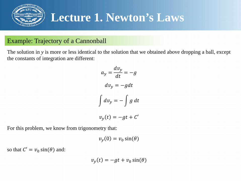
Example: Trajectory of a CannonballThe solution in y is more or less identical to the solution that we obtained above dropping a ball, exceptthe constants of integration are different:

𝑎𝑎𝑦𝑦 =𝑑𝑑𝑣𝑣𝑦𝑦𝑑𝑑𝑡𝑡

= −𝑚𝑚

𝑑𝑑𝑣𝑣𝑦𝑦 = −𝑚𝑚𝑑𝑑𝑡𝑡

�𝑑𝑑𝑣𝑣𝑦𝑦 = −�𝑚𝑚 𝑑𝑑𝑡𝑡

𝑣𝑣𝑦𝑦 𝑡𝑡 = −𝑚𝑚𝑡𝑡 + 𝐶𝐶′

For this problem, we know from trigonometry that:

𝑣𝑣𝑦𝑦 0 = 𝑣𝑣0 sin(𝜃𝜃)

so that 𝐶𝐶′ = 𝑣𝑣0 sin(𝜃𝜃) and:

𝑣𝑣𝑦𝑦 𝑡𝑡 = −𝑚𝑚𝑡𝑡 + 𝑣𝑣0 sin(𝜃𝜃)


Example: Trajectory of a CannonballWe write vy in terms of the time derivative of y and integrate:

𝑑𝑑𝑦𝑦𝑑𝑑𝑡𝑡

= 𝑣𝑣𝑦𝑦 𝑡𝑡 = −𝑚𝑚𝑡𝑡 + 𝑣𝑣0 sin 𝜃𝜃

𝑑𝑑𝑦𝑦 = (−𝑚𝑚𝑡𝑡 + 𝑣𝑣0 sin 𝜃𝜃 )𝑑𝑑𝑡𝑡

�𝑑𝑑𝑦𝑦 = �(−𝑚𝑚𝑡𝑡 + 𝑣𝑣0 sin 𝜃𝜃 )𝑑𝑑𝑡𝑡

𝑦𝑦 𝑡𝑡 = −12𝑚𝑚𝑡𝑡2 + 𝑣𝑣0 sin 𝜃𝜃 𝑡𝑡 + 𝐷𝐷

Again we use y(0) = 0 in the coordinate system we selected to set D = 0 and get:

𝑦𝑦 𝑡𝑡 = −12𝑚𝑚𝑡𝑡2 + 𝑣𝑣0 sin 𝜃𝜃 𝑡𝑡


Example: Trajectory of a CannonballCollecting the results from above, our overall solution is thus:

𝑥𝑥 𝑡𝑡 = 𝑣𝑣0 cos(𝜃𝜃) 𝑡𝑡

𝑦𝑦 𝑡𝑡 = −12𝑚𝑚𝑡𝑡2 + 𝑣𝑣0 sin 𝜃𝜃 𝑡𝑡

𝑣𝑣𝑥𝑥 𝑡𝑡 = 𝑣𝑣0𝑥𝑥 = 𝑣𝑣0 cos𝜃𝜃

𝑣𝑣𝑦𝑦 𝑡𝑡 = −𝑚𝑚𝑡𝑡 + 𝑣𝑣0 sin(𝜃𝜃)

We know exactly where the cannonball is at all times, and we know exactly what its velocity is as well.


The Inclined Plane

In this problem we will talk about a new force, the normal force. Recall from above that thenormal force is whatever magnitude it needs to be to prevent an object from moving in to asolid surface, and is always perpendicular (normal) to that surface in direction.

This is the naive/wrong coordinate system to usefor the inclined plane problem. The problem canbe solved in this coordinate frame, but thesolution (as you can see) would be quite difficult.


The Inclined Plane

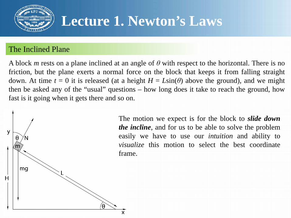
A block m rests on a plane inclined at an angle of θ with respect to the horizontal. There is nofriction, but the plane exerts a normal force on the block that keeps it from falling straightdown. At time t = 0 it is released (at a height H = Lsin(θ) above the ground), and we mightthen be asked any of the “usual” questions – how long does it take to reach the ground, howfast is it going when it gets there and so on.

The motion we expect is for the block to slide downthe incline, and for us to be able to solve the problemeasily we have to use our intuition and ability tovisualize this motion to select the best coordinateframe.


The Inclined Plane

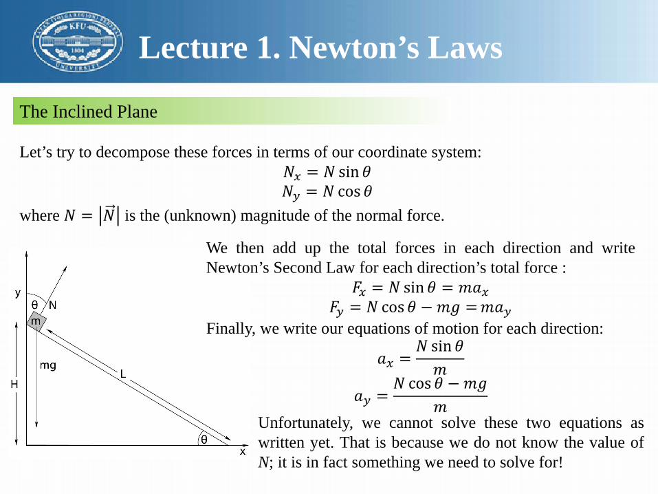
Let’s try to decompose these forces in terms of our coordinate system:𝑁𝑁𝑥𝑥 = 𝑁𝑁 sin𝜃𝜃𝑁𝑁𝑦𝑦 = 𝑁𝑁 cos𝜃𝜃

where 𝑁𝑁 = 𝑁𝑁 is the (unknown) magnitude of the normal force.

We then add up the total forces in each direction and writeNewton’s Second Law for each direction’s total force :

𝐹𝐹𝑥𝑥 = 𝑁𝑁 sin𝜃𝜃 = 𝑚𝑚𝑎𝑎𝑥𝑥𝐹𝐹𝑦𝑦 = 𝑁𝑁 cos𝜃𝜃 − 𝑚𝑚𝑚𝑚 =𝑚𝑚𝑎𝑎𝑦𝑦

Finally, we write our equations of motion for each direction:

𝑎𝑎𝑥𝑥 =𝑁𝑁 sin𝜃𝜃𝑚𝑚

𝑎𝑎𝑦𝑦 =𝑁𝑁 cos𝜃𝜃 −𝑚𝑚𝑚𝑚

𝑚𝑚Unfortunately, we cannot solve these two equations aswritten yet. That is because we do not know the value ofN; it is in fact something we need to solve for!


The Inclined Plane

To solve them we need to add a condition on the solution, expressed as an equation. Thecondition we need to add is that the motion is down the incline, that is, at all times:

𝑦𝑦(𝑡𝑡)𝐿𝐿 cos𝜃𝜃 − 𝑥𝑥(𝑡𝑡)

= tan𝜃𝜃

That means that:𝑦𝑦 𝑡𝑡 = 𝐿𝐿 cos𝜃𝜃 − 𝑥𝑥 𝑡𝑡 tan𝜃𝜃

𝑑𝑑𝑦𝑦(𝑡𝑡)𝑑𝑑𝑡𝑡

= −𝑑𝑑𝑥𝑥 𝑡𝑡𝑑𝑑𝑡𝑡

tan𝜃𝜃𝑑𝑑2𝑦𝑦(𝑡𝑡)𝑑𝑑𝑡𝑡2

= −𝑑𝑑2𝑥𝑥 𝑡𝑡𝑑𝑑𝑡𝑡2

tan𝜃𝜃𝑎𝑎𝑦𝑦 = −𝑎𝑎𝑥𝑥 tan𝜃𝜃

We can use this relation to eliminate (say) ay from the equations above, solve for ax, thenbacksubstitute to find ay.

The solutions we get will be so very complicated (at least compared to choosing a betterframe), with both x and y varying nontrivially with time!

A good choice of coordinate frame has (say) the x-coordinate lined up with the total force and hencedirection of motion.


The Inclined Plane

We can decompose the forces in this coordinatesystem, but now we need to find the components ofthe gravitational force as 𝑁𝑁 = 𝑁𝑁�𝑦𝑦 is easy!Furthermore, we know that ay = 0 and hence Fy = 0.

𝐹𝐹𝑥𝑥 = 𝑚𝑚𝑚𝑚 sin𝜃𝜃 = 𝑚𝑚𝑎𝑎𝑥𝑥𝐹𝐹𝑦𝑦 = 𝑁𝑁 −𝑚𝑚𝑚𝑚 cos𝜃𝜃 = 𝑚𝑚𝑎𝑎𝑦𝑦 = 0

We can immediately solve the y equation for:𝑁𝑁 = 𝑚𝑚𝑚𝑚 cos𝜃𝜃

and write the equation of motion for the x-direction: 𝑎𝑎𝑥𝑥 = 𝑚𝑚 sin𝜃𝜃 which is a constant.From this point on the solution should be familiar – since 𝑣𝑣𝑦𝑦 0 = 0 and 𝑦𝑦 0 = 0, 𝑦𝑦 𝑡𝑡 = 0and we can ignore y altogether and the problem is now one dimensional!See if you can find how long it takes for the block to reach bottom, and how fast it is goingwhen it gets there. You should find that 𝑣𝑣𝑏𝑏𝑠𝑠𝑡𝑡𝑡𝑡𝑠𝑠𝑚𝑚 = 2𝑚𝑚𝐻𝐻


Circular Motion

A small ball, moving in a circle of radius r. We arelooking down from above the circle of motion at aparticle moving counterclockwise around the circle. Atthe moment, at least, the particle is moving at a constantspeed v (so that its velocity is always tangent to thecircle).

The length of a circular arc is the radius times the anglesubtended by the arc we can see that:

∆𝑐𝑐 = 𝑣𝑣∆𝜃𝜃

Note Well! In this and all similar equations θ must bemeasured in radians, never degrees


Circular Motion

The average speed v of the particle is thus this distancedivided by the time it took to move it:

𝑣𝑣𝑎𝑎𝑎𝑎𝑔𝑔 =∆𝑐𝑐∆𝑡𝑡

= 𝑣𝑣∆𝜃𝜃∆𝑡𝑡

Of course, we really don’t want to use average speed (atleast for very long) because the speed might be varying,so we take the limit that Δt → 0 and turn everything intoderivatives, but it is much easier to draw the picturesand visualize what is going on for a small, finite Δt :

𝑣𝑣 = lim∆𝑡𝑡→0

𝑣𝑣∆𝜃𝜃∆𝑡𝑡

= 𝑣𝑣𝑑𝑑𝜃𝜃𝑑𝑑𝑡𝑡

This speed is directed tangent to the circle of motion (asone can see in the figure) and we will often refer to it asthe tangential velocity.


Circular Motion

𝑣𝑣𝑡𝑡 = 𝑣𝑣𝑑𝑑𝜃𝜃𝑑𝑑𝑡𝑡

In this equation, we see that the speed of the particle atany instant is the radius times the rate that the angle isbeing swept out by the particle per unit time. This latterquantity is a very useful one for describing circularmotion, or rotating systems in general.

We define it to be the angular velocity:

𝜔𝜔 =𝑑𝑑𝜃𝜃𝑑𝑑𝑡𝑡

Thus: 𝑣𝑣 = 𝑣𝑣𝜔𝜔 or 𝜔𝜔 = 𝑎𝑎𝑚𝑚


Centripetal Acceleration

A ball of mass m swings down in a circular arc of radius Lsuspended by a string, arriving at the bottom with speed v. Whatis the tension in the string?

At the bottom of the trajectory, the tension T in the string pointsstraight up and the force mg points straight down. No other forcesact, so we should choose coordinates such that one axis lines upwith these two forces. Let’s use +y vertically up, aligned with thestring. Then:

𝐹𝐹𝑦𝑦 = 𝑇𝑇 −𝑚𝑚𝑚𝑚 = 𝑚𝑚𝑎𝑎𝑦𝑦 = 𝑚𝑚𝑣𝑣2

𝐿𝐿

or 𝑇𝑇 = 𝑚𝑚𝑚𝑚 + 𝑚𝑚 𝑎𝑎2

𝐿𝐿

The net force towards the center of the circle must be algebraically equal to mv2/r


Example: Ball on a String

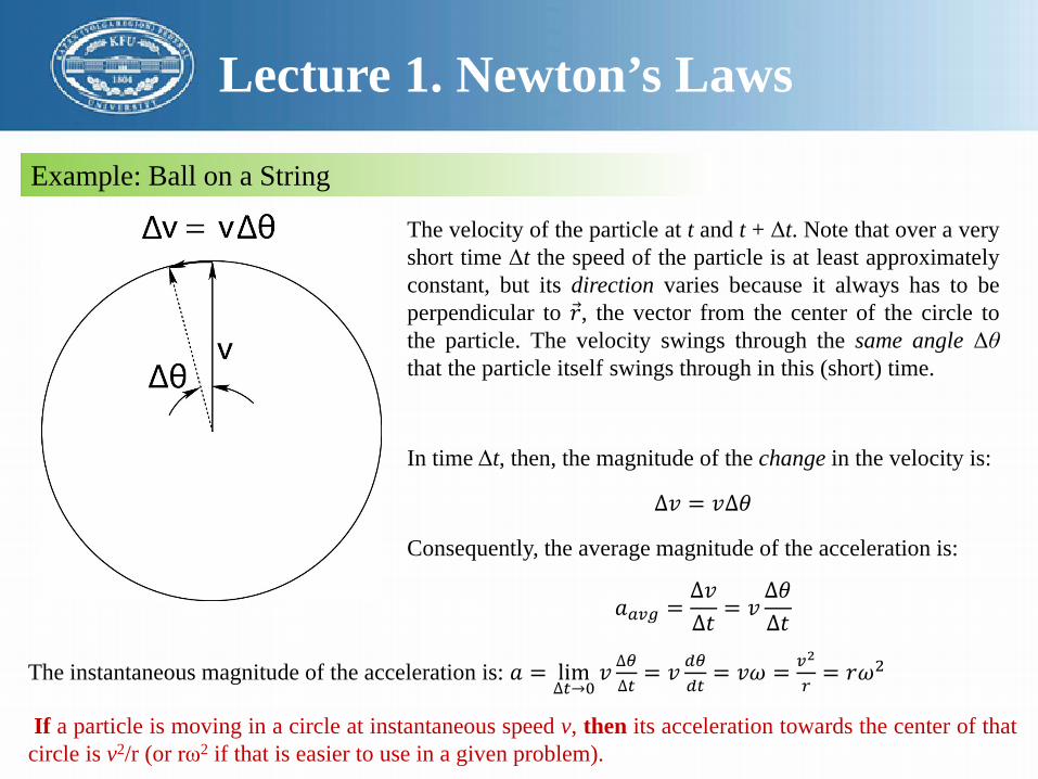
The velocity of the particle at t and t + Δt. Note that over a veryshort time Δt the speed of the particle is at least approximatelyconstant, but its direction varies because it always has to beperpendicular to 𝑣𝑣, the vector from the center of the circle tothe particle. The velocity swings through the same angle Δθthat the particle itself swings through in this (short) time.

In time Δt, then, the magnitude of the change in the velocity is:

∆𝑣𝑣 = 𝑣𝑣∆𝜃𝜃

Consequently, the average magnitude of the acceleration is:

𝑎𝑎𝑎𝑎𝑎𝑎𝑔𝑔 =∆𝑣𝑣∆𝑡𝑡

= 𝑣𝑣∆𝜃𝜃∆𝑡𝑡

The instantaneous magnitude of the acceleration is: 𝑎𝑎 = lim∆𝑡𝑡→0

𝑣𝑣 ∆𝜃𝜃∆𝑡𝑡

= 𝑣𝑣 𝑑𝑑𝜃𝜃𝑑𝑑𝑡𝑡

= 𝑣𝑣𝜔𝜔 = 𝑎𝑎2

𝑚𝑚= 𝑣𝑣𝜔𝜔2

If a particle is moving in a circle at instantaneous speed v, then its acceleration towards the center of thatcircle is v2/r (or rω2 if that is easier to use in a given problem).


Example: Tether Ball/Conic Pendulum

Ball on a rope (a tether ball or conical pendulum). The ballsweeps out a right circular cone at an angle θ with the verticalwhen launched appropriately.

Suppose you hit a tether ball so that it moves in a plane circle atan angle θ at the end of a string of length L. Find T (the tensionin the string) and v, the speed of the ball such that this is true.

Note well in this figure that the only “real” forces acting on theball are gravity and the tension T in the string. Thus in the y-direction we have:

�𝐹𝐹𝑦𝑦 = 𝑇𝑇cos𝜃𝜃 −𝑚𝑚𝑚𝑚 = 0

and in the x-direction (the minus r-direction, as drawn) we have: ∑𝐹𝐹𝑥𝑥 = 𝑇𝑇sin𝜃𝜃 = 𝑚𝑚𝑎𝑎𝑚𝑚 = 𝑚𝑚𝑎𝑎2

𝑚𝑚

Thus 𝑇𝑇 = 𝑚𝑚𝑔𝑔cos 𝜃𝜃

𝑣𝑣2 = 𝑇𝑇𝑚𝑚 sin 𝜃𝜃𝑚𝑚

or 𝑣𝑣 = 𝑚𝑚𝐿𝐿 sin𝜃𝜃 tan𝜃𝜃


Example: Tangential Acceleration

Sometimes we will want to solve problems where a particle speeds up or slows down whilemoving in a circle. Obviously, this means that there is a nonzero tangential accelerationchanging the magnitude of the tangential velocity.

Let’s write �⃗�𝐹 (total) acting on a particle moving in a circle in a coordinate system that rotatesalong with the particle – plane polar coordinates. The tangential direction is the �⃗�𝜃 direction,so we will get:

�⃗�𝐹 = 𝐹𝐹𝑚𝑚�̂�𝑣 + 𝐹𝐹𝜃𝜃�̂�𝜃

From this we will get two equations of motion (connecting this, at long last, to the dynamicsof two dimensional motion):

𝐹𝐹𝑚𝑚 = −𝑚𝑚𝑣𝑣2

𝑣𝑣

𝐹𝐹𝑡𝑡 = 𝑚𝑚𝑎𝑎𝑡𝑡 = 𝑚𝑚𝑑𝑑𝑣𝑣𝑑𝑑𝑡𝑡


Friction

The maximum force static friction can exert is proportional to both the pressure between the surfacesand the area in contact. This makes it proportional to the product of the pressure and the area, whichequals the normal force. We write this as:

𝑓𝑓𝑠𝑠 ≤ 𝑓𝑓𝑠𝑠𝑚𝑚𝑎𝑎𝑥𝑥

= 𝜇𝜇𝑠𝑠𝑁𝑁

where μs is the coefficient of static friction, a dimensionless constant characteristic of the two surfacesin contact, and N is the normal force.

Static Friction is the force exerted by one surface onanother that acts parallel to the surfaces to prevent thetwo surfaces from sliding.

Static friction is as large as it needs to be to prevent anysliding motion, up to a maximum value, at which pointthe surfaces begin to slide.

The frictional force will depend only on the total force, not the area or pressure separately:

𝑓𝑓𝑘𝑘 = 𝜇𝜇𝑘𝑘𝑃𝑃 ∗ 𝐴𝐴 = 𝜇𝜇𝑘𝑘𝑁𝑁𝐴𝐴∗ 𝐴𝐴 = 𝜇𝜇𝑘𝑘𝑁𝑁


Inclined Plane of Length L with Friction

A block of mass m released from rest at time t = 0 on a plane oflength L inclined at an angle θ relative to horizontal is once againgiven, this time more realistically, including the effects of friction.

a) At what angle θc does the block barely overcome theforce of static friction and slide down the incline?

b) Started at rest from an angle θ>θc (so it definitelyslides), how fast will the block be going when itreaches the bottom?


Inclined Plane of Length L with FrictionTo answer the first question, we note that static friction exertsas much force as necessary to keep the block at rest up to themaximum it can exert, 𝑓𝑓𝑠𝑠𝑚𝑚𝑎𝑎𝑥𝑥 = 𝜇𝜇𝑠𝑠𝑁𝑁.

We therefore decompose the known force rules into x and ycomponents, sum them componentwise, write Newton’sSecond Law for both vector components and finally use ourprior knowledge that the system remains in static forceequilibrium to set ax = ay = 0. We get:

�𝐹𝐹𝑥𝑥 = 𝑚𝑚𝑚𝑚 sin𝜃𝜃 − 𝑓𝑓𝑠𝑠 = 0

(for θ ≤ θc and v(0) = 0) and

�𝐹𝐹𝑦𝑦 = 𝑁𝑁 −𝑚𝑚𝑚𝑚 cos𝜃𝜃 = 0

So far, fs is precisely what it needs to be to prevent motion: 𝑓𝑓𝑠𝑠 = 𝑚𝑚𝑚𝑚 sin𝜃𝜃while N = 𝑚𝑚𝑚𝑚 cos𝜃𝜃 . It is true at any angle, moving or not moving, from the Fy equation


Inclined Plane of Length L with FrictionThe critical angle is the angle where fs is as large as it can besuch that the block barely doesn’t slide. To find it, we cansubstitute fs

max = μsNc where Nc = mg cos(θc) into bothequations, so that the first equation becomes:


Inclined Plane of Length L with FrictionThe critical angle is the angle where fs is as large as it can besuch that the block barely doesn’t slide. To find it, we cansubstitute fs

max = μsNc where Nc = mg cos(θc) into bothequations, so that the first equation becomes:

�𝐹𝐹𝑥𝑥 = 𝑚𝑚𝑚𝑚 sin𝜃𝜃𝑠𝑠 − 𝜇𝜇𝑠𝑠𝑚𝑚𝑚𝑚 cos𝜃𝜃𝑠𝑠 = 0

at θc. Solving for θc, we get: θc=tan-1(μs)

Once it is moving then the block will accelerate and Newton’s Second Law becomes:

�𝐹𝐹𝑥𝑥 = 𝑚𝑚𝑚𝑚 sin𝜃𝜃 − 𝜇𝜇𝑘𝑘𝑚𝑚𝑚𝑚 cos𝜃𝜃 = 𝑚𝑚𝑎𝑎𝑥𝑥

which we can solve for the constant acceleration of the block down the incline:𝑎𝑎𝑥𝑥 = 𝑚𝑚 sin𝜃𝜃 − 𝜇𝜇𝑘𝑘𝑚𝑚 cos𝜃𝜃 = 𝑚𝑚 sin𝜃𝜃 − 𝜇𝜇𝑘𝑘 cos𝜃𝜃)

Given ax, it is now straightforward to answer the second question above. For example, we can integrate twice and find vx(t) and x(t), use the latter to find the time it takes to reach the bottom, and substitute that time into the former to find the speed at the bottom of the incline.


Block Hanging off of a Table

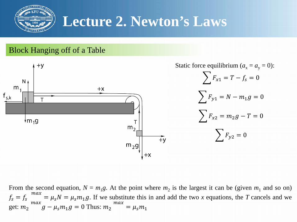
Atwood’s machine, sort of, with one block resting on a table with friction and the other dangling overthe side being pulled down by gravity near the Earth’s surface. Note that we should use an “around thecorner” coordinate system as shown, since a1 = a2 = a if the string is unstretchable.



Suppose a block of mass m1 sits on a table. The coefficients of static and kinetic friction between theblock and the table are μs > μk and μk respectively. This block is attached by an “ideal” masslessunstretchable string running over an “ideal” massless frictionless pulley to a block of mass m2 hangingoff of the table. The blocks are released from rest at time t = 0.

What is the largest that m2 can be before the system starts to move, in terms of the givens andknowns (m1, g, μk, μs...)?



Static force equilibrium (ax = ay = 0):

�𝐹𝐹𝑥𝑥1 = 𝑇𝑇 − 𝑓𝑓𝑠𝑠 = 0

�𝐹𝐹𝑦𝑦1 = 𝑁𝑁 −𝑚𝑚1𝑚𝑚 = 0

�𝐹𝐹𝑥𝑥2 = 𝑚𝑚2𝑚𝑚 − 𝑇𝑇 = 0

�𝐹𝐹𝑦𝑦2 = 0

From the second equation, N = m1g. At the point where m2 is the largest it can be (given m1 and so on)𝑓𝑓𝑠𝑠 = 𝑓𝑓𝑠𝑠

𝑚𝑚𝑎𝑎𝑥𝑥= 𝜇𝜇𝑠𝑠𝑁𝑁 = 𝜇𝜇𝑠𝑠𝑚𝑚1𝑚𝑚. If we substitute this in and add the two x equations, the T cancels and we

get: 𝑚𝑚2𝑚𝑚𝑎𝑎𝑥𝑥

𝑚𝑚 − 𝜇𝜇𝑠𝑠𝑚𝑚1𝑚𝑚 = 0 Thus: 𝑚𝑚2𝑚𝑚𝑎𝑎𝑥𝑥

= 𝜇𝜇𝑠𝑠𝑚𝑚1



If m2 is larger than this minimum, so m1 willslide to the right as m2 falls. We will have tosolve Newton’s Second Law for both massesin order to obtain the non-zero acceleration tothe right and down, respectively:

�𝐹𝐹𝑥𝑥1 = 𝑇𝑇 − 𝑓𝑓𝑘𝑘 = 𝑚𝑚1𝑎𝑎

�𝐹𝐹𝑦𝑦1 = 𝑁𝑁 −𝑚𝑚1𝑚𝑚 = 0

�𝐹𝐹𝑥𝑥2 = 𝑚𝑚2𝑚𝑚 − 𝑇𝑇 = 𝑚𝑚2𝑎𝑎

�𝐹𝐹𝑦𝑦2 = 0

If we substitute the fixed value for 𝑓𝑓𝑘𝑘 = 𝜇𝜇𝑘𝑘𝑁𝑁 = 𝜇𝜇𝑘𝑘𝑚𝑚1𝑚𝑚 and then add the two x equations once again(using the fact that both masses have the same acceleration because the string is unstretchable as noted inour original construction of round-the-corner coordinates), the tension T cancels and we get:𝑚𝑚2𝑚𝑚 − 𝜇𝜇𝑠𝑠𝑚𝑚1𝑚𝑚 = 𝑚𝑚1 + 𝑚𝑚2 𝑎𝑎 or 𝑎𝑎 = 𝑚𝑚2𝑔𝑔−𝜇𝜇𝑠𝑠𝑚𝑚1𝑔𝑔

𝑚𝑚1+𝑚𝑚2


Drag Forces

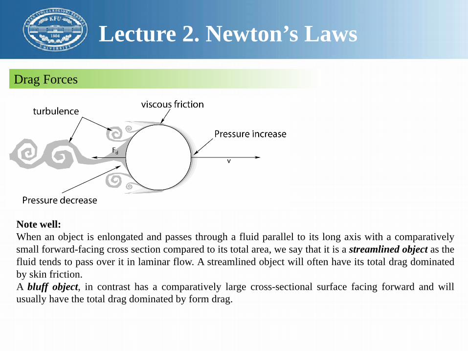
A “cartoon” illustrating the differential force on anobject moving through a fluid.

When the object is moving withrespect to the fluid then weempirically observe that afriction-like force is exerted onthe object called drag.

Drag Force is the “frictional”force exerted by a fluid (liquid orgas) on an object that movesthrough it. Like kinetic friction, italways opposes the direction ofrelative motion of the object andthe medium

Note well: When an object is enlongated and passes through a fluid parallel to its long axis with acomparatively small forward-facing cross section compared to its total area, we say that it is astreamlined object as the fluid tends to pass over it in laminar flow. A streamlined object will often haveits total drag dominated by skin friction. A bluff object, in contrast has a comparatively large cross-sectional surface facing forward and will usually have the total drag dominated by form drag.


Drag Forces

Note well:When an object is enlongated and passes through a fluid parallel to its long axis with a comparativelysmall forward-facing cross section compared to its total area, we say that it is a streamlined object as thefluid tends to pass over it in laminar flow. A streamlined object will often have its total drag dominatedby skin friction.A bluff object, in contrast has a comparatively large cross-sectional surface facing forward and willusually have the total drag dominated by form drag.


Drag Forces

Drag is an extremely complicated force. It depends on a vast array of things including but not limited to:

• The size of the object.• The shape of the object.• The relative velocity of the object through the fluid.• The state of the fluid (e.g. its velocity field including any internal turbulence).• The density of the fluid.• The viscosity of the fluid (we will learn what this is later).• The properties and chemistry of the surface of the object (smooth versus rough, strong or weak

chemical interaction with the fluid at the molecular level).• The orientation of the object as it moves through the fluid, which may be fixed in time (streamlined

versus bluff motion) or varying in time (as, for example, an irregularly shaped object tumbles).

To eliminate most of this complexity and end up with “force rules” that will often be quantitativelypredictive we will use a number of idealizations. We will only consider smooth, uniform, nonreactivesurfaces of convex bluff objects (like spheres) or streamlined objects (like rockets or arrows) movingthrough uniform, stationary fluids where we can ignore or treat separately the other non-drag (e.g.buoyant) forces acting on the object.


Drag Forces

There are two dominant contributions to drag for objects of this sort.

The first, as noted above, is form drag – the difference in pressure times projective area between thefront of an object and the rear of an object. It is strongly dependent on both the shape and orientation ofan object and requires at least some turbulence in the trailing wake in order to occur.

The second is skin friction, the friction-like force resulting from the fluid rubbing across the skin atright angles in laminar flow.


Stokes, or Laminar Drag

The first is when the object is moving through the fluid relatively slowly and/or is arrow-shaped orrocket-ship-shaped so that streamlined laminar drag (skin friction) is dominant. In this case there isrelatively little form drag, and in particular, there is little or no turbulence – eddies of fluid spinningaround an axis – in the wake of the object as the presence of turbulence (which we will discuss in moredetail later when we consider fluid dynamics) breaks up laminar flow.

This “low-velocity, streamlined” skin friction drag is technically named Stokes’ drag or laminar dragand has the idealized force rule:

�⃗�𝐹𝑑𝑑 = −𝑏𝑏�⃗�𝑣This is the simplest sort of drag – a drag force directly proportional to the velocity of relative motion ofthe object through the fluid and oppositely directed.

Stokes derived the following relation for the dimensioned number bl (the laminar drag coefficient)that appears in this equation for a sphere of radius R:

𝑏𝑏𝑙𝑙 = −6𝜋𝜋𝜇𝜇𝜋𝜋where μ is the dynamical viscosity.


Rayleigh, or Turbulent Drag

On the other hand, if one moves an object through a fluid too fast – where the actual speed depends indetail on the actual size and shape of the object, how bluff or streamlined it is – pressure builds up onthe leading surface and turbulence appears in its trailing wake in the fluid.

This high velocity, turbulent drag exerts a force described by a quadratic dependence on the relativevelocity due to Lord Rayleigh:

�⃗�𝐹𝑑𝑑 = −12𝜌𝜌𝐶𝐶𝑑𝑑𝐴𝐴 𝑣𝑣 �⃗�𝑣 = −𝑏𝑏𝑡𝑡 𝑣𝑣 �⃗�𝑣

It is still directed opposite to the relative velocity of the object and the fluid but now is proportional tothat velocity squared. In this formula ρ is the density of the fluid through which the object moves (sodenser fluids exert more drag as one would expect) and A is the cross-sectional area of the objectperpendicular to the direction of motion, also known as the orthographic projection of the object on anyplane perpendicular to the motion. For example, for a sphere of radius R, the orthographic projection is acircle of radius R and the area A = πR2.The number Cd is called the drag coefficient and is a dimensionless number that depends on relativespeed, flow direction, object position, object size, fluid viscosity and fluid density.


Example: Falling From a Plane and Surviving

Suppose you fall from a large height (long enough to reach terminal velocity) to hit ahaystack of height H that exerts a nice, uniform force to slow you down all the way to theground, smoothly compressing under you as you fall. In that case, your initial velocity at thetop is vt, down. In order to stop you before y = 0 (the ground) you have to have a netacceleration −a such that:

𝑣𝑣 𝑡𝑡𝑔𝑔 = 0 = 𝑣𝑣𝑡𝑡 − 𝑎𝑎𝑡𝑡𝑔𝑔

𝑦𝑦 𝑡𝑡𝑔𝑔 = 0 = 𝐻𝐻 − 𝑣𝑣𝑡𝑡𝑡𝑡𝑔𝑔 −12𝑎𝑎𝑡𝑡𝑔𝑔2

If we solve the first equation for tg and substitute it into the second and solve for themagnitude of a, we will get:

−𝑣𝑣𝑡𝑡2= −2𝑎𝑎𝐻𝐻 or 𝑎𝑎 = 𝑎𝑎𝑡𝑡2

2𝐻𝐻We know also that 𝐹𝐹ℎ𝑎𝑎𝑦𝑦𝑠𝑠𝑡𝑡𝑎𝑎𝑠𝑠𝑘𝑘 − 𝑚𝑚𝑚𝑚 = 𝑚𝑚𝑎𝑎 or

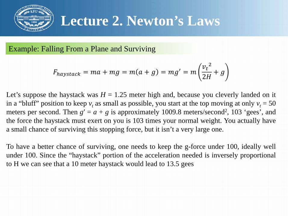
𝐹𝐹ℎ𝑎𝑎𝑦𝑦𝑠𝑠𝑡𝑡𝑎𝑎𝑠𝑠𝑘𝑘 = 𝑚𝑚𝑎𝑎 + 𝑚𝑚𝑚𝑚 = 𝑚𝑚 𝑎𝑎 + 𝑚𝑚 = 𝑚𝑚𝑚𝑚′ = 𝑚𝑚𝑣𝑣𝑡𝑡2

2𝐻𝐻+ 𝑚𝑚


Example: Falling From a Plane and Surviving

𝐹𝐹ℎ𝑎𝑎𝑦𝑦𝑠𝑠𝑡𝑡𝑎𝑎𝑠𝑠𝑘𝑘 = 𝑚𝑚𝑎𝑎 + 𝑚𝑚𝑚𝑚 = 𝑚𝑚 𝑎𝑎 + 𝑚𝑚 = 𝑚𝑚𝑚𝑚′ = 𝑚𝑚𝑣𝑣𝑡𝑡2

2𝐻𝐻+ 𝑚𝑚

Let’s suppose the haystack was H = 1.25 meter high and, because you cleverly landed on itin a “bluff” position to keep vt as small as possible, you start at the top moving at only vt = 50meters per second. Then g′ = a + g is approximately 1009.8 meters/second2, 103 ‘gees’, andthe force the haystack must exert on you is 103 times your normal weight. You actually havea small chance of surviving this stopping force, but it isn’t a very large one.

To have a better chance of surviving, one needs to keep the g-force under 100, ideally wellunder 100. Since the “haystack” portion of the acceleration needed is inversely proportionalto H we can see that a 10 meter haystack would lead to 13.5 gees

Lecture 3. Work and Energy

Work and Kinetic Energy

If you integrate a constant acceleration of an object twice, you obtain:𝑣𝑣 𝑡𝑡 = 𝑎𝑎𝑡𝑡 + 𝑣𝑣0

𝑥𝑥 𝑡𝑡 =12𝑎𝑎𝑡𝑡2 + 𝑣𝑣0𝑡𝑡 + 𝑥𝑥0

where v0 is the initial speed and x0 is the initial x position at time t = 0.

Now, suppose you want to find the speed v1 the object will have when it reaches position x1.One can algebraically, once and for all note that this must occur at some time t1 such that:

𝑣𝑣 𝑡𝑡1 = 𝑎𝑎𝑡𝑡1 + 𝑣𝑣0 = 𝑣𝑣1𝑥𝑥 𝑡𝑡1 =

12𝑎𝑎𝑡𝑡12 + 𝑣𝑣0𝑡𝑡1 + 𝑥𝑥0 = 𝑥𝑥1

We can algebraically solve the first equation once and for all for t1:𝑡𝑡1 =

𝑣𝑣1 − 𝑣𝑣0𝑎𝑎

and substitute the result into the second equation, eliminating time altogether from thesolutions:


Work and Kinetic Energy12𝑎𝑎𝑣𝑣1 − 𝑣𝑣0

𝑎𝑎

2+ 𝑣𝑣0

𝑣𝑣1 − 𝑣𝑣0𝑎𝑎

+ 𝑥𝑥0 = 𝑥𝑥1

12𝑎𝑎(𝑣𝑣1

2−2𝑣𝑣0𝑣𝑣1 + 𝑣𝑣02) +𝑣𝑣0𝑣𝑣1 − 𝑣𝑣02

𝑎𝑎= 𝑥𝑥1 − 𝑥𝑥0

𝑣𝑣12 − 2𝑣𝑣0𝑣𝑣1 + 𝑣𝑣02 + 2𝑣𝑣0𝑣𝑣1 − 𝑣𝑣02 = 2𝑎𝑎(𝑥𝑥1 − 𝑥𝑥0)or 𝑣𝑣12 − 𝑣𝑣02 = 2𝑎𝑎(𝑥𝑥1 − 𝑥𝑥0)

Lets consider a constant acceleration in one dimension only:𝑣𝑣12 − 𝑣𝑣02 = 2𝑎𝑎∆𝑥𝑥

If we multiply by m (the mass of the object) and move the annoying 2 over to the other side, we canmake the constant acceleration a into a constant force Fx = ma:

𝑚𝑚𝑎𝑎 ∆𝑥𝑥 =12𝑚𝑚𝑣𝑣12 −

12𝑚𝑚𝑣𝑣02

𝐹𝐹𝑥𝑥∆𝑥𝑥 =12𝑚𝑚𝑣𝑣12 −

12𝑚𝑚𝑣𝑣02

We now define the work done by the constant force Fx on the mass m as it moves through the distanceΔx to be: ∆𝑊𝑊 = 𝐹𝐹𝑥𝑥∆𝑥𝑥Work is a form of energy.

1 Joule = 1 Newton � meter = 1kilogram � meter2

second2


Kinetic Energy

Let’s define the quantity changed by the work to be the kinetic energy and will usethe symbol K to represent it in this work:

𝐾𝐾 =12𝑚𝑚𝑣𝑣2

Work-Kinetic Energy Theorem:The work done on a mass by the total force acting on it is equal to the change in itskinetic energy.

and as an equation that is correct for constant one dimensional forces only:

∆𝑊𝑊 = 𝐹𝐹𝑥𝑥∆𝑥𝑥 =12𝑚𝑚𝑣𝑣𝑓𝑓2 −

12𝑚𝑚𝑣𝑣𝑖𝑖2 = ∆𝐾𝐾


Conservative Forces: Potential Energy

We define a conservative force to be one such that the work done by the force as you move apoint mass from point �⃗�𝑥1 to point �⃗�𝑥2 is independent of the path used to move between the points:

𝑊𝑊𝑙𝑙𝑠𝑠𝑠𝑠𝑙𝑙 = ��⃗�𝑥1(path 1)

�⃗�𝑥2�⃗�𝐹 � 𝑑𝑑𝑙𝑙 = �

�⃗�𝑥1(path 2)

�⃗�𝑥2�⃗�𝐹 � 𝑑𝑑𝑙𝑙

In this case (only), the work done going around an arbitrary closed path (starting and endingon the same point) will be identically zero!

𝑊𝑊𝑙𝑙𝑠𝑠𝑠𝑠𝑙𝑙 = �𝐶𝐶�⃗�𝐹 � 𝑑𝑑𝑙𝑙 = 0

The work done going around an arbitrary loop by aconservative force is zero. This ensures that the workdone going between two points is independent of thepath taken, its defining characteristic.


Conservative Forces: Potential Energy

Since the work done moving a mass m from an arbitrary starting point to any point in spaceis the same independent of the path, we can assign each point in space a numerical value: thework done by us on mass m, against the conservative force, to reach it.This is the negative of the work done by the force. We do it with this sign for reasons thatwill become clear in a moment. We call this function the potential energy of the mass massociated with the conservative force �⃗�𝐹:

𝑈𝑈 �⃗�𝑥 = −�𝑥𝑥0

𝑥𝑥�⃗�𝐹 � 𝑑𝑑�⃗�𝑥 = −𝑊𝑊

Note Well: that only one limit of integration depends on x; the other depends on where youchoose to make the potential energy zero. This is a free choice. No physical result that can bemeasured or observed can uniquely depend on where you choose the potential energy to bezero.


Conservation of Mechanical Energy

The principle of the Conservation of Mechanical Energy:The total mechanical energy (defined as the sum of its potential and kinetic energies) ofa particle being acted on by only conservative forces is constant.Or, if only conservative forces act on an object and U is the potential energy function for thetotal conservative force, then

𝐸𝐸𝑚𝑚𝑚𝑚𝑠𝑠ℎ = 𝐾𝐾 + 𝑈𝑈 = 𝐴𝐴 scalar constant

The fact that the force is the negative derivative of the potential energy of an object meansthat the force points in the direction the potential energy decreases in.


Example: Falling Ball Reprise

To see how powerful this is, let us look back at a fallingobject of mass m (neglecting drag and friction). First, wehave to determine the gravitational potential energy of theobject a height y above the ground (where we will chooseto set U(0) = 0):

𝑈𝑈 𝑦𝑦 = −�0

𝑦𝑦−𝑚𝑚𝑚𝑚 𝑑𝑑𝑦𝑦 = 𝑚𝑚𝑚𝑚𝑦𝑦

Now, suppose we have our ball of mass m at the height Hand drop it from rest. How fast is it going when it hits theground? This time we simply write the total energy of theball at the top (where the potential is mgH and the kineticis zero) and the bottom (where the potential is zero andkinetic is 1

2𝑚𝑚𝑣𝑣2 and set the two equal! Solve for v, done:

𝐸𝐸𝑖𝑖 = 𝑚𝑚𝑚𝑚𝐻𝐻 + 0 = 0 +12𝑚𝑚𝑣𝑣2 = 𝐸𝐸𝑓𝑓

or 𝑣𝑣 = 2𝑚𝑚𝐻𝐻


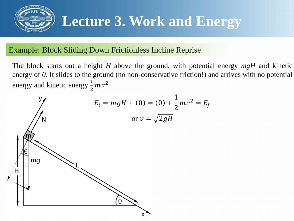
Example: Block Sliding Down Frictionless Incline Reprise

The block starts out a height H above the ground, with potential energy mgH and kineticenergy of 0. It slides to the ground (no non-conservative friction!) and arrives with no potentialenergy and kinetic energy 1

2𝑚𝑚𝑣𝑣2

𝐸𝐸𝑖𝑖 = 𝑚𝑚𝑚𝑚𝐻𝐻 + 0 = 0 +12𝑚𝑚𝑣𝑣2 = 𝐸𝐸𝑓𝑓

or 𝑣𝑣 = 2𝑚𝑚𝐻𝐻


Example: Looping the Loop

What is the minimum height H such that a block of mass m loops-the-loop (stays on thefrictionless track all the way around the circle)?



Here we need two physical principles: Newton’s Second Law and the kinematics of circularmotion since the mass is undoubtedly moving in a circle if it stays on the track. Here’s theway we reason:“If the block moves in a circle of radius R at speed v, then its acceleration towards the centermust be ac = v2/R. Newton’s Second Law then tells us that the total force component in thedirection of the center must be mv2/R. That force can only be made out of (a component of)gravity and the normal force, which points towards the center. So we can relate the normalforce to the speed of the block on the circle at any point.”At the top (where we expect v to be at its minimum value, assuming it stays on the circle)gravity points straight towards the center of the circle of motion, so we get:

𝑚𝑚𝑚𝑚 + 𝑁𝑁 =𝑚𝑚𝑣𝑣2

𝜋𝜋and in the limit that N → 0 (“barely” looping the loop) we get the condition:

𝑚𝑚𝑚𝑚 =𝑚𝑚𝑣𝑣𝑡𝑡2

𝜋𝜋where vt is the (minimum) speed at the top of the track needed to loop the loop.



Now we need to relate the speed at the top of the circle to the original height H it began at.This is where we need our third principle – Conservation of Mechanical Energy!With energy we don’t care about the shape of the track, only that the track do no work onthe mass which (since it is frictionless and normal forces do no work) is in the bag. Thus:

𝐸𝐸𝑖𝑖 = 𝑚𝑚𝑚𝑚𝐻𝐻 = 𝑚𝑚𝑚𝑚2𝜋𝜋 +12𝑚𝑚𝑣𝑣𝑡𝑡2 = 𝐸𝐸𝑓𝑓

If you put these two equations together (e.g. solve the first for 𝑚𝑚𝑣𝑣𝑡𝑡2 and substitute it into thesecond, then solve for H in terms of R) you should get

Hmin = 5R/2.


Example: Generalized Work-Mechanical Energy Theorem

Let’s consider what happens if both conservative and nonconservative forces are acting on a particle. In that case the argument above becomes:

𝑊𝑊𝑚𝑚𝑠𝑠𝑡𝑡 = 𝑊𝑊𝐶𝐶 + 𝑊𝑊𝑁𝑁𝐶𝐶 = ∆𝐾𝐾

or 𝑊𝑊𝑁𝑁𝐶𝐶 = ∆𝐾𝐾 −𝑊𝑊𝐶𝐶 = ∆𝐾𝐾 + ∆𝑈𝑈 = ∆𝐸𝐸𝑚𝑚𝑚𝑚𝑠𝑠ℎ

which we state as the Generalized Non-Conservative Work-Mechanical EnergyTheorem:

The work done by all the non-conservative forces acting on a particle equals the changein its total mechanical energy.


Example: Heat and Conservation of Energy

The important empirical law is the Law of Conservation of Energy. Whenever we examine aphysical system and try very hard to keep track of all of the mechanical energy exchangeswithin that system and between the system and its surroundings, we find that we can alwaysaccount for them all without any gain or loss.

In other words, we find that the total mechanical energy of an isolated system never changes,and if we add or remove mechanical energy to/from the system, it has to come from or go tosomewhere outside of the system. This result, applied to well defined systems of particles,can be formulated as the First Law of Thermodynamics:

∆𝑄𝑄𝑖𝑖𝑠𝑠 = ∆𝐸𝐸𝑠𝑠𝑓𝑓 + 𝑊𝑊𝑏𝑏𝑦𝑦

In words, the heat energy flowing in to a system equals the change in the internal totalmechanical energy of the system plus the external work (if any) done by the system on itssurroundings.


Example: Heat and Conservation of Energy

When a block slides down a rough table from some initial velocity to rest, kinetic frictionturns the bulk organized kinetic energy of the collectively moving mass into disorganizedmicroscopic energy – heat.

As the rough microscopic surfaces bounce off of one another and form and break chemicalbonds, it sets the actual molecules of the block bounding, increasing the internal microscopicmechanical energy of the block and warming it up.


Power

The energy in a given system is not, of course, usually constant in time. Energy is added to agiven mass, or taken away, at some rate.

There are many times when we are given the rate at which energy is added or removed intime, and need to find the total energy added or removed. This rate is called the power.

Power: The rate at which work is done, or energy released into a system.

𝑑𝑑𝑊𝑊 = �⃗�𝐹𝑑𝑑�⃗�𝑥 = �⃗�𝐹 �𝑑𝑑𝑥𝑥𝑑𝑑𝑡𝑡𝑑𝑑𝑡𝑡

𝑃𝑃 =𝑑𝑑𝑊𝑊𝑑𝑑𝑡𝑡

= �⃗�𝐹 � �⃗�𝑣

so that ∆𝑊𝑊 = ∆𝐸𝐸𝑡𝑡𝑠𝑠𝑡𝑡 = ∫𝑃𝑃𝑑𝑑𝑡𝑡

The units of power are clearly Joules/sec = Watts. Another common unit of power is“Horsepower”, 1 HP = 746 W.


Equilibrium

The force is given by the negative gradient of the potential energy:

�⃗�𝐹 = −𝛻𝛻𝑈𝑈

or (in each direction): 𝐹𝐹𝑥𝑥 = −𝑑𝑑𝑑𝑑𝑑𝑑𝑥𝑥

,𝐹𝐹𝑦𝑦 = −𝑑𝑑𝑑𝑑𝑑𝑑𝑦𝑦

, 𝐹𝐹𝑧𝑧 = −𝑑𝑑𝑑𝑑𝑑𝑑𝑧𝑧

,

or the force is the negative slope of the potential energy function in this direction.

The meaning of this is that if a particle moves in the direction of the (conservative) force, itspeeds up. If it speeds up, its kinetic energy increases. If its kinetic energy increases, itspotential energy must decrease. The force (component) acting on a particle is thus the rate atwhich the potential energy decreases (the negative slope) in any given direction


Equilibrium

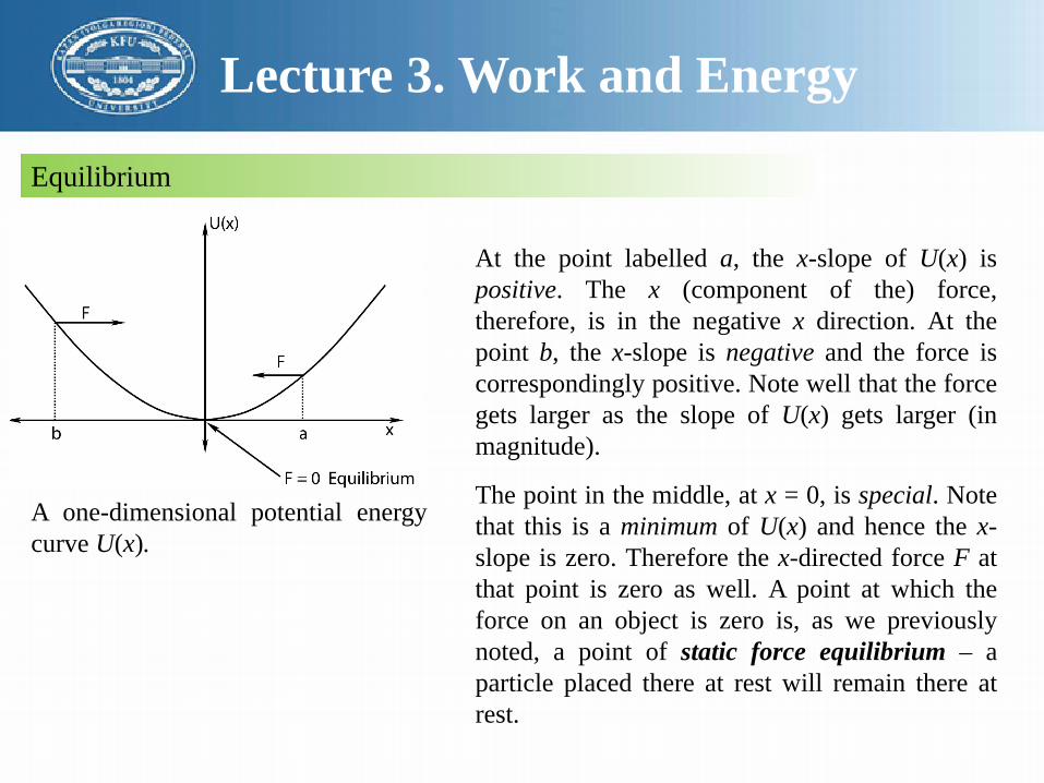
A one-dimensional potential energy curve U(x).


Equilibrium

A one-dimensional potential energycurve U(x).

At the point labelled a, the x-slope of U(x) ispositive. The x (component of the) force,therefore, is in the negative x direction. At thepoint b, the x-slope is negative and the force iscorrespondingly positive. Note well that the forcegets larger as the slope of U(x) gets larger (inmagnitude).

The point in the middle, at x = 0, is special. Notethat this is a minimum of U(x) and hence the x-slope is zero. Therefore the x-directed force F atthat point is zero as well. A point at which theforce on an object is zero is, as we previouslynoted, a point of static force equilibrium – aparticle placed there at rest will remain there atrest.


Equilibrium

A one-dimensional potential energycurve U(x).

In this particular figure, if one moves the particlea small distance to the right or the left of theequilibrium point, the force pushes the particleback towards equilibrium. Points where the forceis zero and small displacements cause a restoringforce in this way are called stable equilibriumpoints. As you can see, the isolated minima of apotential energy curve (or surface, in higherdimensions) are all stable equilibria.


Equilibrium

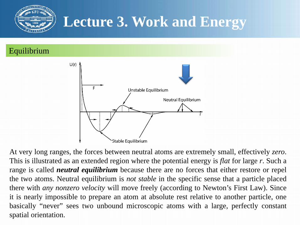
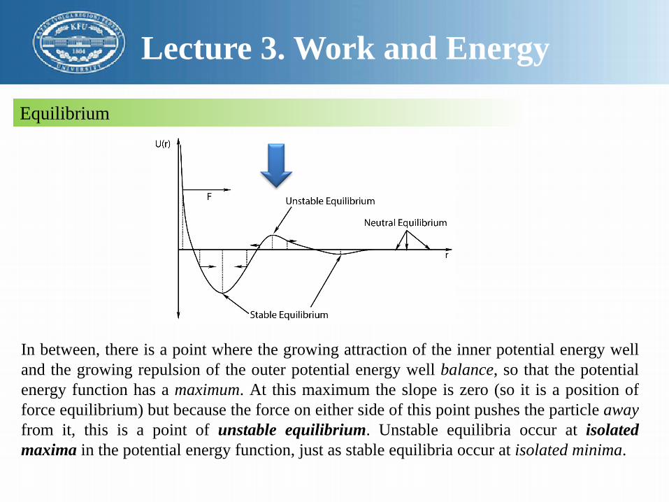
A fairly generic potential energy shape for microscopic (atomic or molecular) interactions,drawn to help exhibits features one might see in such a curve more than as a realisticallyscaled potential energy in some set of units. In particular, the curve exhibits stable, unstable,and neutral equilibria for a radial potential energy as a function of r, the distance between twoe.g. atoms.


Equilibrium

At very long ranges, the forces between neutral atoms are extremely small, effectively zero.This is illustrated as an extended region where the potential energy is flat for large r. Such arange is called neutral equilibrium because there are no forces that either restore or repelthe two atoms. Neutral equilibrium is not stable in the specific sense that a particle placedthere with any nonzero velocity will move freely (according to Newton’s First Law). Sinceit is nearly impossible to prepare an atom at absolute rest relative to another particle, onebasically “never” sees two unbound microscopic atoms with a large, perfectly constantspatial orientation.


Equilibrium

As the two atoms near one another, their interaction becomes first weakly attractive due toe.g. quantum dipole-induced dipole interactions and then weakly repulsive as the two atomsstart to “touch” each other. There is a potential energy minimum in between where twoatoms separated by a certain distance can be in stable equilibrium without being chemicallybound.


Equilibrium

Atoms that approach one another still more closely encounter a second potential energywell that is at first strongly attractive followed by a hard core repulsion as the electronclouds are prevented from interpenetrating by e.g. the Pauli exclusion principle. Thissecond potential energy well is often modelled by a Lennard-Jones potential energy It alsohas a point of stable equilibrium.


Equilibrium

In between, there is a point where the growing attraction of the inner potential energy welland the growing repulsion of the outer potential energy well balance, so that the potentialenergy function has a maximum. At this maximum the slope is zero (so it is a position offorce equilibrium) but because the force on either side of this point pushes the particle awayfrom it, this is a point of unstable equilibrium. Unstable equilibria occur at isolatedmaxima in the potential energy function, just as stable equilibria occur at isolated minima.

Lecture 4. Systems of Particles,Momentum and Collisions. Statics

Systems of Particles

An object such as a baseball is not really a particle. It is made of many, many particles – eventhe atoms it is made of are made of many particles each. Yet it behaves like a particle as far asNewton’s Laws are concerned.

We will obtain this collective behavior by averaging, or summing over at successively largerscales, the physics that we know applies at the smallest scale to things that really are particles.


Newton’s Laws for a System of Particles – Center of Mass

A system of N = 3 particles is shown, with various forces�⃗�𝐹𝑖𝑖 acting on the masses (which therefore each their ownaccelerations �⃗�𝑎𝑖𝑖). From this, we construct a weightedaverage acceleration of the system, in such a way thatNewton’s Second Law is satisfied for the total mass.

Suppose we have a system of N particles, each of which is experiencing a force. Some (part)of those forces are “external” – they come from outside of the system. Some (part) of themmay be “internal” – equal and opposite force pairs between particles that help hold the systemtogether (solid) or allow its component parts to interact (liquid or gas).



We would like the total force to act on the total mass ofthis system as if it were a “particle”. That is, we wouldlike for:

�⃗�𝐹𝑡𝑡𝑠𝑠𝑡𝑡 = 𝑀𝑀𝑡𝑡𝑠𝑠𝑡𝑡𝐴𝐴

where 𝐴𝐴 is the “acceleration of the system”. Newton’sSecond Law for a system of particles is written as:

�⃗�𝐹𝑡𝑡𝑠𝑠𝑡𝑡 = �𝑖𝑖

�⃗�𝐹𝑖𝑖 =�𝑖𝑖

𝑚𝑚𝑖𝑖𝑑𝑑2�⃗�𝑥𝑖𝑖𝑑𝑑𝑡𝑡2

=

= �𝑖𝑖

𝑚𝑚𝑖𝑖𝑑𝑑2𝑋𝑋𝑑𝑑𝑡𝑡2

= 𝑀𝑀𝑡𝑡𝑠𝑠𝑡𝑡𝑑𝑑2𝑋𝑋𝑑𝑑𝑡𝑡2

= 𝑀𝑀𝑡𝑡𝑠𝑠𝑡𝑡𝐴𝐴



�𝑖𝑖


= 𝑀𝑀𝑡𝑡𝑠𝑠𝑡𝑡𝑑𝑑2𝑋𝑋𝑑𝑑𝑡𝑡2

Basically, if we define an 𝑋𝑋 such that this relation is true then Newton’s second law is recoveredfor the entire system of particles “located at 𝑋𝑋” as if that location were indeed a particle of massMtot itself. We can rearrange this a bit as:

𝑑𝑑𝑉𝑉𝑑𝑑𝑡𝑡

=𝑑𝑑2𝑋𝑋𝑑𝑑𝑡𝑡2

=1

𝑀𝑀𝑡𝑡𝑠𝑠𝑡𝑡�𝑖𝑖


=1


𝑚𝑚𝑖𝑖𝑑𝑑�⃗�𝑣𝑖𝑖𝑑𝑑𝑡𝑡

and can integrate twice on both sides. The first integral is:

𝑑𝑑𝑋𝑋𝑑𝑑𝑡𝑡

= 𝑉𝑉 =1


𝑚𝑚𝑖𝑖�⃗�𝑣𝑖𝑖 + 𝑉𝑉0 =1


𝑚𝑚𝑖𝑖𝑑𝑑�⃗�𝑥𝑖𝑖𝑑𝑑𝑡𝑡

+ 𝑉𝑉0

and the second is: 𝑋𝑋 = 1𝑀𝑀𝑡𝑡𝑡𝑡𝑡𝑡

∑𝑖𝑖 𝑚𝑚𝑖𝑖�⃗�𝑥𝑖𝑖 + 𝑉𝑉0𝑡𝑡 + 𝑋𝑋0



We define the position of the center of mass to be:

𝑀𝑀𝑋𝑋cm = ∑𝑖𝑖𝑚𝑚𝑖𝑖�⃗�𝑥𝑖𝑖 or 𝑋𝑋cm = 1𝑀𝑀∑𝑖𝑖𝑚𝑚𝑖𝑖�⃗�𝑥𝑖𝑖

Not all systems we treat will appear to be made up of point particles. Most solid objects orfluids appear to be made up of a continuum of mass, a mass distribution. In this case weneed to do the sum by means of integration, and our definition becomes:

𝑀𝑀𝑋𝑋cm = ∫ �⃗�𝑥𝑑𝑑𝑚𝑚 or 𝑋𝑋cm = 1𝑀𝑀 ∫ �⃗�𝑥𝑑𝑑𝑚𝑚


Momentum

Momentum is a useful idea that follows naturally from our decision to treat collections as objects. It is a way of combining the mass (which is a characteristic of the object) with the velocity of the object. We define the momentum to be:

�⃗�𝑝 = 𝑚𝑚�⃗�𝑣Thus (since the mass of an object is generally constant):

�⃗�𝐹 = 𝑚𝑚�⃗�𝑎 = 𝑚𝑚𝑑𝑑�⃗�𝑣𝑑𝑑𝑡𝑡

=𝑑𝑑𝑑𝑑𝑡𝑡

𝑚𝑚�⃗�𝑣 =𝑑𝑑�⃗�𝑝𝑑𝑑𝑡𝑡

is another way of writing Newton’s second law.Note that there exist systems (like rocket ships, cars, etc.) where the mass is not constant. Asthe rocket rises, its thrust (the force exerted by its exhaust) can be constant, but it continuallygets lighter as it burns fuel. Newton’s second law (expressed as �⃗�𝐹 = 𝑚𝑚�⃗�𝑎) does tell us what todo in this case – but only if we treat each little bit of burned and exhausted gas as a “particle”,which is a pain. On the other hand, Newton’s second law expressed as �⃗�𝐹 = 𝑑𝑑�⃗�𝑙

𝑑𝑑𝑡𝑡still works fine

and makes perfect sense – it simultaneously describes the loss of mass and the increase ofvelocity as a function of the mass correctly.


Momentum

Clearly we can repeat our previous argument for the sum of the momenta of a collection of particles:

𝑃𝑃𝑡𝑡𝑠𝑠𝑡𝑡 = �𝑖𝑖

�⃗�𝑝𝑖𝑖 = �𝑖𝑖

𝑚𝑚�⃗�𝑣𝑖𝑖

so that

𝑑𝑑𝑃𝑃𝑡𝑡𝑠𝑠𝑡𝑡𝑑𝑑𝑡𝑡

= �𝑖𝑖

�⃗�𝑝𝑖𝑖𝑑𝑑𝑡𝑡

= �𝑖𝑖

�⃗�𝐹𝑖𝑖 = �⃗�𝐹𝑡𝑡𝑠𝑠𝑡𝑡

Differentiating our expression for the position of the center of mass above, we also get:𝑑𝑑∑𝑖𝑖𝑚𝑚�⃗�𝑥𝑖𝑖

𝑑𝑑𝑡𝑡= �

𝑖𝑖

𝑚𝑚𝑑𝑑�⃗�𝑥𝑖𝑖𝑑𝑑𝑡𝑡

=�𝑖𝑖

�⃗�𝑝𝑖𝑖 = 𝑃𝑃𝑡𝑡𝑠𝑠𝑡𝑡 = 𝑀𝑀𝑡𝑡𝑠𝑠𝑡𝑡�⃗�𝑣𝑠𝑠𝑚𝑚


The Law of Conservation of Momentum

We are now in a position to state and trivially prove the Law of Conservation of Momentum.

If and only if the total external force acting on a system is zero, then the total momentum of a system (of particles) is a constant vector.

You are welcome to learn this in its more succinct algebraic form:

If and only if �⃗�𝐹𝑡𝑡𝑠𝑠𝑡𝑡 = 0 then 𝑃𝑃𝑡𝑡𝑠𝑠𝑡𝑡 = 𝑃𝑃𝑖𝑖𝑠𝑠𝑖𝑖𝑡𝑡𝑖𝑖𝑎𝑎𝑙𝑙 = 𝑃𝑃𝑓𝑓𝑖𝑖𝑠𝑠𝑎𝑎𝑙𝑙 = a constant vector.


Impulse

As the surfaces of the two (hard) balls come into contact, they “suddenly” exert relativelylarge, relatively violent, equal and opposite forces on each other over a relatively short time,and then the force between the objects once again drops to zero as they either bounce apart orstick together and move with a common velocity.“Relatively” here in all cases means compared to all other forces acting on the system duringthe collision in the event that those forces are not actually zero.

Let us imagine a typical collision: one pool ballapproaches and strikes another, causing bothballs to recoil from the collision in some(probably different) directions and at differentspeeds. Before they collide, they are widelyseparated and exert no force on one another.


Impulse

Let us begin, then, by defining the average force over the (short) time Δt of any givencollision, assuming that we did know �⃗�𝐹 = �⃗�𝐹21(𝑡𝑡), the force one object (say m1) exerts on theother object (m2).The magnitude of such a force (one perhaps appropriate to the collision of pool balls) issketched below in figure where for simplicity we assume that the force acts only along the lineof contact and is hence effectively one dimensional in this direction.

The time average of this force iscomputed the same way the timeaverage of any other timedependentquantity might be:


Impulse

The time average of this force is computed the same way the time average of any othertime-dependent quantity might be:

�⃗�𝐹𝑎𝑎𝑎𝑎𝑔𝑔 =1∆𝑡𝑡�0

∆𝑡𝑡�⃗�𝐹 𝑡𝑡 𝑑𝑑𝑡𝑡

We can evaluate the integral using Newton’s Second Law expressed in terms of momentum:

�⃗�𝐹 𝑡𝑡 =𝑑𝑑�⃗�𝑝𝑑𝑑𝑡𝑡

so that (multiplying out by dt and integrating):

�⃗�𝑝2𝑓𝑓 − �⃗�𝑝2𝑖𝑖 = ∆�⃗�𝑝2 = �0

∆𝑡𝑡�⃗�𝐹 𝑡𝑡 𝑑𝑑𝑡𝑡

Note that the momentum change of the first ball is equal and opposite. From Newton’sThird Law, �⃗�𝐹12 𝑡𝑡 = −�⃗�𝐹21 𝑡𝑡 = �⃗�𝐹 and:

�⃗�𝑝1𝑓𝑓 − �⃗�𝑝1𝑖𝑖 = ∆�⃗�𝑝1 = −�0

∆𝑡𝑡�⃗�𝐹 𝑡𝑡 𝑑𝑑𝑡𝑡 = −∆�⃗�𝑝2


Impulse

The integral of a force �⃗�𝐹 over an interval of time is called the impulse imparted by the force

𝐼𝐼 = �𝑡𝑡1

𝑡𝑡2�⃗�𝐹 𝑡𝑡 𝑑𝑑𝑡𝑡 = �

𝑡𝑡1

𝑡𝑡2 𝑑𝑑�⃗�𝑝𝑑𝑑𝑡𝑡

𝑡𝑡 𝑑𝑑𝑡𝑡 = �𝑙𝑙1

𝑙𝑙2𝑑𝑑�⃗�𝑝 = �⃗�𝑝2 − �⃗�𝑝1 =∆�⃗�𝑝

This proves that the (vector) impulse is equal to the (vector) change in momentum over thesame time interval, a result known as the impulse-momentum theorem. From our point ofview, the impulse is just the momentum transferred between two objects in a collision insuch a way that the total momentum of the two is unchanged.Returning to the average force, we see that the average force in terms of the impulse is just:

�⃗�𝐹𝑎𝑎𝑎𝑎𝑔𝑔 =𝐼𝐼∆𝑡𝑡

=∆𝑝𝑝∆𝑡𝑡

=�⃗�𝑝𝑓𝑓 − �⃗�𝑝𝑖𝑖∆𝑡𝑡


Impulse, Fluids, and Pressure

Another valuable use of impulse is when we have many objects colliding with something –so many that even though each collision takes only a short time Δt, there are so manycollisions that they exert a nearly continuous force on the object.This is critical to understanding the notion of pressure exerted by a fluid, becausemicroscopically the fluid is just a lot of very small particles that are constantly collidingwith a surface and thereby transferring momentum to it, so many that they exert a nearlycontinuous and smooth force on it that is the average force exerted per particle times thenumber of particles that collide.

Suppose you have a cube with sides of length Lcontaining N molecules of a gas.



Let’s suppose that all of the molecules have a mass m and an average speed in the x directionof vx, with (on average) one half going left and one half going right at any given time.In order to be in equilibrium (so vx doesn’t change) the change in momentum of any moleculethat hits, say, the right hand wall perpendicular to x is Δpx = 2mvx. This is the impulsetransmitted to the wall per molecular collision. To find the total impulse in the time Δt, onemust multiply this by one half the number of molecules in in a volume L2vx Δt. That is,

∆𝑝𝑝𝑡𝑡𝑠𝑠𝑡𝑡 =12

𝑁𝑁𝐿𝐿3

𝐿𝐿2𝑣𝑣𝑥𝑥∆𝑡𝑡(2𝑚𝑚𝑣𝑣𝑥𝑥)

Let’s call the volume of the box L3 = V and the area of the wall receiving the impulse L2 = A.

𝑃𝑃 =𝐹𝐹𝑎𝑎𝑎𝑎𝑔𝑔𝐴𝐴

=∆𝑝𝑝𝑡𝑡𝑠𝑠𝑡𝑡𝐴𝐴∆𝑡𝑡

=𝑁𝑁𝑉𝑉

12𝑚𝑚𝑣𝑣𝑥𝑥2 =

𝑁𝑁𝑉𝑉

𝐾𝐾𝑥𝑥,𝑎𝑎𝑎𝑎𝑔𝑔

where the average force per unit area applied to the wall is the pressure, which has SI units ofNewtons/meter2 or Pascals.



If we add a result called the equipartition theorem:

𝐾𝐾𝑥𝑥,𝑎𝑎𝑎𝑎𝑔𝑔 =12𝑚𝑚𝑣𝑣𝑥𝑥2 =

12𝑘𝑘𝑏𝑏𝑇𝑇2

∆𝑝𝑝𝑡𝑡𝑠𝑠𝑡𝑡 =12

𝑁𝑁𝐿𝐿3

𝐿𝐿2𝑣𝑣𝑥𝑥∆𝑡𝑡(2𝑚𝑚𝑣𝑣𝑥𝑥)

where kb is Boltzmann’s constant and T is the temperature in degrees absolute, one gets:𝑃𝑃𝑉𝑉 = 𝑁𝑁𝑘𝑘𝑇𝑇

which is the Ideal Gas Law.


Collisions

A “collision” in physics occurs when two bodies that are more or less not interacting (becausethey are too far apart to interact) come “in range” of their mutual interaction force, stronglyinteract for a short time, and then separate so that they are once again too far apart to interact.

There are three general “types” of collision:• Elastic• Fully Inelastic• Partially Inelastic


Elastic collisionBy definition, an elastic collision is one that also conserves total kinetic energy so that thetotal scalar kinetic energy of the colliding particles before the collision must equal the totalkinetic energy after the collision. This is an additional independent equation that the solutionmust satisfy.

General relationships:

1. Conservation of momentum �⃗�𝑝1𝑖𝑖 + �⃗�𝑝2𝑖𝑖 = �⃗�𝑝1𝑓𝑓 + �⃗�𝑝2𝑓𝑓

2. Conservation of kinetic energy: 12𝑚𝑚1�⃗�𝑣1𝑖𝑖2 + 1

2𝑚𝑚2�⃗�𝑣2𝑖𝑖2 = 1

2𝑚𝑚1�⃗�𝑣𝑓𝑓2

′ + 12𝑚𝑚2�⃗�𝑣2𝑓𝑓2

3. For head-on collisions: 𝑣𝑣1′ = (𝑚𝑚1−𝑚𝑚2)(𝑚𝑚1−𝑚𝑚2)

𝑣𝑣1 ; 𝑣𝑣2′ = 2𝑚𝑚1(𝑚𝑚1+𝑚𝑚2)

𝑣𝑣1

4. For head-on collisions the velocity of approach is equal to the velocity of separation


Inelastic collisionA fully inelastic collision is where two particles collide and stick together. As always,momentum is conserved in the impact approximation, but now kinetic energy is not!

�⃗�𝑝𝑖𝑖,𝑠𝑠 𝑡𝑡𝑠𝑠𝑡𝑡 = 𝑚𝑚1�⃗�𝑣1𝑖𝑖 + 𝑚𝑚2�⃗�𝑣2𝑖𝑖 = 𝑚𝑚1 + 𝑚𝑚2 �⃗�𝑣𝑓𝑓 = 𝑚𝑚1 + 𝑚𝑚2 �⃗�𝑣𝑠𝑠𝑚𝑚 = �⃗�𝑝𝑓𝑓,𝑡𝑡𝑠𝑠𝑡𝑡

In other words, in a fully inelastic collision, the velocity of the outgoing combined particle isthe velocity of the center of mass of the system, which we can easily compute from aknowledge of the initial momenta or velocities and masses.


Example: Ballistic Pendulum

The “ballistic pendulum”, where a bullet strikes andsticks to/in a block, which then swings up to amaximum angle θf before stopping and swinging backdown.The classic ballistic pendulum question gives you themass of the block M, the mass of the bullet m, thelength of a string or rod suspending the “target” blockfrom a free pivot, and the initial velocity of the bulletv0. It then asks for the maximum angle θf through whichthe pendulum swings after the bullet hits and sticks tothe block (or alternatively, the maximum height Hthrough which it swings).

Solution:During the collision momentum is conserved in the impact approximation, which in thiscase basically implies that the block has no time to swing up appreciably “during” theactual collision.


Example: Ballistic Pendulum

Solution:• During the collision momentum is conserved in the

impact approximation, which in this case basically impliesthat the block has no time to swing up appreciably“during” the actual collision.

• After the collision mechanical energy is conserved.Mechanical energy is not conserved during the collision(see solution above of straight up inelastic collision).

Momentum conservation: 𝑝𝑝𝑚𝑚,0 = 𝑚𝑚𝑣𝑣0 = 𝑝𝑝𝑀𝑀+𝑚𝑚,𝑓𝑓

kinetic part of mechanical energy conservation in terms of momentum:

𝐸𝐸0 =𝑝𝑝𝐵𝐵+𝑏𝑏,𝑓𝑓2

2(𝑀𝑀 + 𝑚𝑚)=

𝑝𝑝𝑏𝑏,02

2(𝑀𝑀 + 𝑚𝑚)= 𝐸𝐸𝑓𝑓 = 𝑀𝑀 + 𝑚𝑚 𝑚𝑚𝐻𝐻 = 𝑀𝑀 + 𝑚𝑚 𝑚𝑚𝜋𝜋(1 − cos𝜃𝜃𝑓𝑓)

Thus: 𝜃𝜃𝑓𝑓 = cos−1(1 − 𝑚𝑚𝑎𝑎0 2

2 𝑀𝑀+𝑚𝑚 2𝑔𝑔𝑔𝑔) which only has a solution if mv0 is less than some

maximum value.


Torque and Rotation

Rotations in One Dimension are rotations of a solid object about a single axis. Since we arefree to choose any arbitrary coordinate system we wish in a problem, we can without loss ofgenerality select a coordinate system where the z-axis represents the (positive or negative)direction or rotation, so that the rotating object rotates “in” the xy plane. Rotations of a rigidbody in the xy plane can then be described by a single angle θ, measured by convention inthe counterclockwise direction from the positive x-axis.

Time-dependent Rotations can thus be described by:a) The angular position as a function of time, θ(t).b) The angular velocity as a function of time,

𝑤𝑤 𝑡𝑡 =𝑑𝑑𝜃𝜃𝑑𝑑𝑡𝑡

c) The angular acceleration as a function of time,

𝛼𝛼 𝑡𝑡 =𝑑𝑑𝑤𝑤𝑑𝑑𝑡𝑡

=𝑑𝑑2𝜃𝜃𝑑𝑑𝑡𝑡2


Torque and Rotation

• Forces applied to a rigid object perpendicular to a line drawn from an axis of rotationexert a torque on the object. The torque is given by:

𝜏𝜏 = 𝑣𝑣𝐹𝐹 sin 𝜑𝜑 = 𝑣𝑣𝐹𝐹⊥ = 𝑣𝑣⊥𝐹𝐹• The torque (as we shall see) is a vector quantity and by convention its direction is

perpendicular to the plane containing 𝑣𝑣 and �⃗�𝐹 in the direction given by the right handrule. Although we won’t really work with this until next week, the “proper” definition ofthe torque is:

𝜏𝜏 = 𝑣𝑣 × �⃗�𝐹• Newton’s Second Law for Rotation in one dimension is:

𝜏𝜏 = 𝐼𝐼𝛼𝛼where I is the moment of inertia of the rigid body being rotated by the torque about agiven/specified axis of rotation. The direction of this (one dimensional) rotation is therighthanded direction of the axis – the direction your right handed thumb points if you graspthe axis with your fingers curling around the axis in the direction of the rotation or torque.


Torque and Rotation

• The moment of inertia of a point particle of mass m located a (fixed) distance r fromsome axis of rotation is:

𝐼𝐼 = 𝑚𝑚𝑣𝑣2

• The moment of inertia of a rigid collection of point particles is:

𝐼𝐼 = �𝑖𝑖

𝑚𝑚𝑖𝑖𝑣𝑣𝑖𝑖2

• The moment of inertia of a continuous solid rigid object is:

𝐼𝐼 = �𝑣𝑣2𝑑𝑑𝑚𝑚

• The rotational kinetic energy of a rigid body (total kinetic energy of all of the chunks ofmass that make it up) is:

𝐾𝐾𝑚𝑚𝑠𝑠𝑡𝑡 =12𝐼𝐼𝑤𝑤2


Conditions for Static Equilibrium

An object at rest remains at rest unless acted on by a net external force.Previously we showed that Newton’s Second Law also applies to systems of particles, withthe replacement of the position of the particle by the position of the center of mass of thesystem and the force with the total external force acting on the entire system.

We also learned that the force equilibrium of particles acted on by conservative forceoccurred at the points where the potential energy was maximum or minimum or neutral(flat), where we named maxima “unstable equilibrium points”, minima “stable equilibriumpoints” and flat regions “neutral equilibria”.

However, we learned enough to now be able to see that force equilibrium alone is notsufficient to cause an extended object or collection of particles to be in equilibrium. We caneasily arrange situations where two forces act on an object in opposite directions (so there isno net force) but along lines such that together they exert a nonzero torque on the object andhence cause it to angularly accelerate and gain kinetic energy without bound, hardly acondition one would call “equilibrium”.


Conditions for Static Equilibrium

The Newton’s Second Law for Rotation is sufficient to imply Newton’s First Law forRotation:

If, in an inertial reference frame, a rigid object is initially at rotational rest (notrotating), it will remain at rotational rest unless acted upon by a net external torque.

That is, 𝜏𝜏 = 𝐼𝐼�⃗�𝛼 = 0 implies 𝑤𝑤 = 0 and constant. We will call the condition where 𝜏𝜏 = 0 anda rigid object is not rotating torque equilibrium.

Therefore we now define the conditions for the static equilibrium of a rigid body to be:

A rigid object is in static equilibrium when both the vector torque and the vector forceacting on it are zero.

That is:

If 𝑭𝑭𝒕𝒕𝒕𝒕𝒕𝒕 = 𝟎𝟎 and 𝝉𝝉𝒕𝒕𝒕𝒕𝒕𝒕 = 𝟎𝟎, then an object initially at translational and rotational restwill remain at rest and neither accelerate nor rotate.


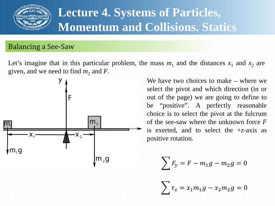
Balancing a See-Saw

You are given m1, x1, and x2 and are asked to find m2 and F such that the see-saw is in staticequilibrium.

One typical problem in statics is balancing weights on a see-saw type arrangement – auniform plank supported by a fulcrum in the middle. This particular problem is really onlyone dimensional as far as force is concerned, as there is no force acting in the x-direction orz-direction.


Balancing a See-Saw

Let’s imagine that in this particular problem, the mass m1 and the distances x1 and x2 aregiven, and we need to find m2 and F.

We have two choices to make – where weselect the pivot and which direction (in orout of the page) we are going to define tobe “positive”. A perfectly reasonablechoice is to select the pivot at the fulcrumof the see-saw where the unknown force Fis exerted, and to select the +z-axis aspositive rotation.

�𝐹𝐹𝑦𝑦 = 𝐹𝐹 −𝑚𝑚1𝑚𝑚 −𝑚𝑚2𝑚𝑚 = 0

�𝜏𝜏𝑧𝑧 = 𝑥𝑥1𝑚𝑚1𝑚𝑚 − 𝑥𝑥2𝑚𝑚2𝑚𝑚 = 0


Balancing a See-Saw

�𝐹𝐹𝑦𝑦 = 𝐹𝐹 −𝑚𝑚1𝑚𝑚 −𝑚𝑚2𝑚𝑚 = 0

�𝜏𝜏𝑧𝑧 = 𝑥𝑥1𝑚𝑚1𝑚𝑚 − 𝑥𝑥2𝑚𝑚2𝑚𝑚 = 0

𝑚𝑚2 =𝑚𝑚1𝑚𝑚𝑥𝑥1𝑚𝑚𝑥𝑥2

=𝑥𝑥1𝑥𝑥2

𝑚𝑚1

From the first equation and the solution for m2:

𝐹𝐹 = 𝑚𝑚1𝑚𝑚 + 𝑚𝑚2𝑚𝑚 = 𝑚𝑚1𝑚𝑚 1 + 𝑥𝑥1𝑥𝑥2

= 𝑚𝑚1𝑚𝑚𝑥𝑥1+𝑥𝑥2𝑥𝑥2


Tipping

Another important application of the ideas of static equilibrium is to tipping problems. Atippingproblem is one where one uses the ideas of static equilibrium to identify theparticular angle or force combination that will marginally cause some object to tip over.

The idea of tipping is simple enough. An object placed on a flat surface is typically stableas long as the center of gravity is vertically inside the edges that are in contact with thesurface, so that the torque created by the gravitational force around this limiting pivot isopposed by the torque exerted by the (variable) normal force.


Tipping Versus Slipping

A rectangular block either tips first or slips(slides down the incline) first as the inclineis gradually increased. Which one happensfirst? The figure is show with the blockjust past the tipping angle.

At some angle we know that the block will start to slide. This will occur because the normal force is decreasing with the angle (and hence, so is the maximum force static friction can exert) and at the same time, the component of the weight of the object that points down the incline is increasing. Eventually the latter will exceed the former and the block will slide.However, at some angle the block will also tip over. We know that this will happen becausethe normal force can only prevent the block from rotating clockwise (as drawn) around thepivot consisting of the lower left corner of the block.



The tipping point, or tipping angle is thus the angle wherethe center of gravity is directly over the pivot that theobject will “tip” around as it falls over.

Let’s find the slipping angle θs. Let “down” mean “down the incline”. Then:

�𝐹𝐹𝑑𝑑𝑠𝑠𝑑𝑑𝑠𝑠 = 𝑚𝑚𝑚𝑚 sin 𝜃𝜃 − 𝐹𝐹𝑠𝑠 = 0

�𝐹𝐹⊥ = 𝑁𝑁 −𝑚𝑚𝑚𝑚 cos 𝜃𝜃 = 0

From the latter, as usual: 𝑁𝑁 = 𝑚𝑚𝑚𝑚 cos 𝜃𝜃 and 𝐹𝐹𝑠𝑠 ≤ 𝐹𝐹𝑠𝑠𝑚𝑚𝑎𝑎𝑥𝑥 = 𝜇𝜇𝑠𝑠𝑁𝑁When 𝑚𝑚𝑚𝑚 sin 𝜃𝜃𝑠𝑠 = 𝐹𝐹𝑠𝑠𝑚𝑚𝑎𝑎𝑥𝑥 = 𝜇𝜇𝑠𝑠𝑁𝑁 cos 𝜃𝜃𝑠𝑠The force of gravity down the incline precisely balances the force of static friction. We can solve for the angle where this occurs:𝜃𝜃𝑠𝑠 = tan−1(𝜇𝜇𝑠𝑠)This happens when the center of mass passes directly over the pivot.



From inspection of the figure (which is drawn very close tothe tipping point) it should be clear that the tipping angle𝜃𝜃𝑡𝑡 is given by:

𝜃𝜃𝑡𝑡 = tan−1𝑊𝑊𝐻𝐻

So, which one wins? The smaller of the two, θs or θt, ofcourse – that’s the one that happens first as the plank israised. Indeed, since both are inverse tangents, the smallerof: 𝜇𝜇𝑠𝑠, W/H

determines whether the system slips first or tips first, noneed to actually evaluate any tangents or inverse tangents!

Lecture 5. Fluids

General Fluid Properties

Fluids are the generic name given to two states of matter, liquids and gases characterized by alack of long range order and a high degree of mobility at the molecular scale.

A large number of atoms or molecules are confined within in a “box”, where they bouncearound off of each other and the walls. They exert a force on the walls equal and oppositethe force the walls exert on them as the collisions more or less elastically reverse theparticles’ momenta perpendicular to the walls.

Lecture 5. Fluids

General Fluid Properties

Many particles all of mass m are constantly moving inrandom, constantly changing directions (as the particlescollide with each other and the walls) with an averagekinetic energy related to the temperature of the fluid.Some of the particles (which might be atoms such ashelium or neon or molecules such as H2 or O2) happen tobe close to the walls of the container and moving in theright direction to bounce (elastically) off of those walls.

When they do, their momentum perpendicular to those walls is reversed. Since many, many ofthese collisions occur each second, there is a nearly continuous momentum transfer betweenthe walls and the gas and the gas and the walls. This transfer, per unit time, becomes theaverage force exerted by the walls on the gas and the gas on the walls

Eventually, we will transform this simple picture into the Kinetic Theory of Gases and use itto derive the venerable Ideal Gas Law

𝑃𝑃𝑉𝑉 = 𝑁𝑁𝑘𝑘𝑏𝑏𝑇𝑇

Lecture 5. Fluids

PressureTo describe the forces that confine and act on the fluids in terms of pressure, defined to be the forceper unit area with which a fluid pushes on a confining wall or the confining wall pushes on the fluid:

𝑃𝑃 =𝐹𝐹𝐴𝐴

Pressure gets its own SI units, which clearly must be Newtons per square meter. We give these unitstheir own name, Pascals:

1 Pascal =Newtonmeter2

A Pascal is a tiny unit of pressure – a Newton isn’t very big, recall (one kilogram weighs roughly tenNewtons) so a Pascal is the weight of a quarter pound spread out over a square meter.

A more convenient measure of pressure in our everyday world is a form of the unit called a bar:

1bar = 105 Pa = 100 kPa

Lecture 5. Fluids

PressureThe average air pressure at sea level is very nearly 1 bar.

The symbol atm stands for one standard atmosphere. The connection between atmospheres, bars, andpascals is:

1 standard atmosphere = 101.325 kPa = 1013.25 mbar

The extra significant digits therefore refer only to a fairly arbitrary value (in pascals) historicallyrelated to the original definition of a standard atmosphere in terms of “millimeters of mercury” or torr :

1 standard atmosphere = 760.00 mmHg = 760.00 torr

In this class we will use the simple rule 1 bar ≈ 1 atm

Note well: in the field of medicine blood pressures are given in mm of mercury (or torr) by longstanding tradition (largely because for at least a century blood pressure was measured with a mercury-based sphygmomanometer). These can be converted into atmospheres by dividing by 760,remembering that one is measuring the difference between these pressures and the standard atmosphere(so the actual blood pressure is always greater than one atmosphere).

Lecture 5. Fluids

DensityEven a very tiny volume of fluid has many, many atoms or molecules in it.

We can work to create a vacuum – a volume that has relatively few molecules in it per unit volume, butit is almost impossible to make that number zero – even the hard vacuum of outer space has on averageone molecule per cubic meter or thereabouts. We live at the bottom of a gravity well that confines ouratmosphere – the air that we breathe – so that it forms a relatively thick soup that we move through andbreathe with order of Avogadro’s Number (6 × 1023) molecules per liter – hundreds of billions ofbillions per cubic centimeter.

At this point we cannot possibly track the motion and interactions of all of the individual molecules, sowe coarse grain and average.

The properties of oxygen molecules and helium molecules might well be very different, so themolecular count alone may not be the most useful quantity. Since we are interested in how forces mightact on these small volumes, we need to know their mass, and thus we define the density of a fluid to be:

𝜌𝜌 =𝑑𝑑𝑚𝑚𝑑𝑑𝑉𝑉

Lecture 5. Fluids

Compressibility

A major difference between fluids and solids, and liquids and gases within the fluids, is thecompressibility of these materials. Compressibility describes how a material responds tochanges in pressure.

This can be expressed as a simple linear relationship:

∆𝑃𝑃 = −𝐵𝐵∆𝑉𝑉𝑉𝑉

Pressure up, volume down and vice versa. The constant of proportionality B is called thebulk modulus of the material.

Note well that we haven’t really specified yet whether the “material” is solid, liquid or gas.All three of them have densities, all three of them have bulk moduli. Where they differ is inthe qualitative properties of their compressibility.

Lecture 5. Fluids

Compressibility

• Solids are typically relatively incompressible (large B), although there are certainly exceptions.They have long range order – all of the molecules are packed and tightly bonded together instructures and there is usually very little free volume.

• Liquids are also relatively incompressible (large B). They differ from solids in that they lack longrange order. All of the molecules are constantly moving around and any small “structures” thatappear due to local interaction are short-lived. The molecules of a liquid are close enough togetherthat there is often significant physical and chemical interaction, giving rise to surface tension andwetting properties – especially in water, which is an amazing fluid!

• Gases are in contrast quite compressible (small B). One can usually squeeze gases smoothly intosmaller and smaller volumes, until they reach the point where the molecules are basically alltouching and the gas converts to a liquid! Gases per se (especially hot gases) usually remain“weakly interacting” right up to where they become a liquid, although the correct (non-ideal)equation of state for a real gas often displays features that are the results of moderate interaction,depending on the pressure and temperature.

Lecture 5. Fluids

Compressibility

Water is, as noted, a remarkable liquid. H2O is apolar molecules with a permanent dipole moment,so water molecules are very strongly interacting,both with each other and with other materials. Itorganizes itself quickly into a state of relative orderthat is very incompressible.

The bulk modulus of water is 2.2 × 109 Pa, which means that even deep in the ocean wherepressures can be measured in the tens of millions of Pascals (or hundreds of atmospheres)the density of water only varies by a few percent from that on the surface. Its density variesmuch more rapidly with temperature than with pressure.

We will idealize water by considering it to be perfectly incompressible in this course, whichis close enough to true for nearly any mundane application of hydraulics that you are mostunlikely to ever observe an exception that matters.

Lecture 5. Fluids

Viscosity and fluid flow

Fluids, whether liquid or gas, have some internal “stickiness” that resists the relative motionof one part of the fluid compared to another, a kind of internal “friction” that tries toequilibrate an entire body of fluid to move together. They also interact with the walls of anycontainer in which they are confined.

The viscosity of a fluid (symbol μ) is a measure of this internal friction or stickiness. Thinfluids have a low viscosity and flow easily with minimum resistance; thick sticky fluidshave a high viscosity and resist flow.

Fluid, when flowing through (say) a cylindrical pipe tends to organize itself in one of twovery different ways – a state of laminar flow where the fluid at the very edge of the flowingvolume is at rest where it is in contact with the pipe and the speed concentrically andsymmetrically increases to a maximum in the center of the pipe, and turbulent flow wherethe fluid tumbles and rolls and forms eddies as it flows through the pipe. Turbulence andflow and viscosity are properties that will be discussed in more detail below.

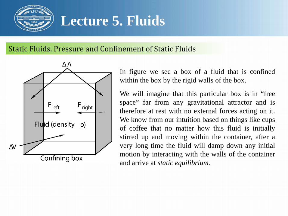
Lecture 5. Fluids

Static Fluids. Pressure and Confinement of Static Fluids

In figure we see a box of a fluid that is confinedwithin the box by the rigid walls of the box.

We will imagine that this particular box is in “freespace” far from any gravitational attractor and istherefore at rest with no external forces acting on it.We know from our intuition based on things like cupsof coffee that no matter how this fluid is initiallystirred up and moving within the container, after avery long time the fluid will damp down any initialmotion by interacting with the walls of the containerand arrive at static equilibrium.

Lecture 5. Fluids


Fluid rotation is more complex than the rotation of a static object because a fluid can beinternally rotating even if all of the fluid in the outermost layer is in contact with a containand is stationary. It can also be turbulent – there can be lots of internal eddies and swirls ofmotion, including some that can exist at very small length scales and persist for fair amountsof time.

We will idealize all of this – when we discuss static properties of fluids we will assume thatall of this sort of internal motion has disappeared.

A fluid in static equilibrium has the property that every singletiny chunk of volume in the fluid has to independently be inforce equilibrium – the total force acting on the differentialvolume chunk must be zero.

In addition the net torques acting on all of these differentialsubvolumes must be zero, and the fluid must be at rest, neithertranslating nor rotating.

Lecture 5. Fluids


Suppose (as shown) the cross-sectional area of the left and right walls are ΔA originally.Consider now what we expect if we double the size of the box and at the same time addenough additional fluid for the fluid density to remain the same, making the side walls havethe area 2 Δ A. With twice the area (and twice the volume and twice as much fluid), we havetwice as many molecular collisions per unit time on the doubled wall areas (with the sameaverage impulse per collision). The average force exerted by the doubled wall areas thereforealso doubles.

We can now make a few very simple observations about theforces exerted by the walls of the container on the fluid within.First of all the mass of the fluid in the box above is clearly:

∆𝑀𝑀 = 𝜌𝜌∆𝑉𝑉

We drew a symmetric box to make it easy to see that themagnitudes of the forces exerted by opposing walls are equalFleft = Fright (for example). Similarly the forces exerted by the topand bottom surfaces, and the front and back surfaces, mustcancel.

Lecture 5. Fluids


An important property of fluids is that one part of a fluid can move independent of anotherso the fluid in at least some layer with a finite thickness near the wall would thereforeexperience a net force and would accelerate. But this violates our assumption of staticequilibrium, so a fluid in static equilibrium exerts no tangential force on the walls of aconfining container and vice versa.We therefore conclude that the direction of the force exerted by a confining surface with anarea ΔA on the fluid that is in contact with it is: �⃗�𝐹 = 𝑃𝑃∆𝐴𝐴�𝑠𝑠. Where �𝑠𝑠 is an inward-directedunit vector perpendicular to (normal to) the surface.

From this simple argument we can conclude that the averageforce exerted by any wall is proportional to the area of the wall.This force is therefore most naturally expressible in terms ofpressure:

𝐹𝐹left = 𝑃𝑃left∆𝐴𝐴 = 𝑃𝑃right∆𝐴𝐴 = 𝐹𝐹rightwhich implies that the pressure at the left and right confiningwalls is the same:

𝑃𝑃left = 𝑃𝑃right = 𝑃𝑃

Lecture 5. Fluids

Pressure and Confinement of Static Fluids in Gravity

The principle change brought about by setting our box of fluid down on the ground in agravitational field is that an additional external force comes into play: The weight of thefluid. A static fluid, confined in some way in a gravitational field, must support the weightof its many component parts internally, and of course the box itself must support theweight of the entire mass ΔM of the fluid.

As hopefully you can see if you carefully read the previous section. The only forceavailable to provide the necessary internal support or confinement force is the variation ofpressure within the fluid. We would like to know how the pressure varies as we move upor down in a static fluid so that it supports its own weight.

If we consider a tiny (eventually differentially small) chunk of fluid in force equilibrium,gravity will pull it down and the only thing that can push it up is a pressure differencebetween the top and the bottom of the chunk.

Lecture 5. Fluids


A fluid in static equilibrium confined to a sealed rectilinear box in a near-Earthgravitational field �⃗�𝑚. Note well the small chunk of fluid with dimensions Δx, Δy, Δz in themiddle of the fluid. Also note that the coordinate system selected has z increasing from thetop of the box down, so that z can be thought of as the depth of the fluid.

Lecture 5. Fluids


In figure a (portion of) a fluid confined to a box is illustrated. The box could be a completelysealed one with rigid walls on all sides, or it could be something like a cup or bucket that isopen on the top but where the fluid is still confined there by e.g. atmospheric pressure.

Let us consider a small (eventually infinitesimal) chunk of fluid somewhere in the middle ofthe container. As shown, it has physical dimensions Δx, Δy, Δz; its upper surface is a distancez below the origin (where z increases down and hence can represent “depth”) and its lowersurface is at depth z + Δz. The areas of the top and bottom surfaces of this small chunk aree.g. ΔAtb = ΔxΔy, the areas of the sides are ΔxΔz and ΔyΔz respectively, and the volume ofthis small chunk is ΔV = Δx ΔyΔz.

This small chunk is itself in static equilibrium – therefore the forces between any pair of itshorizontal sides (in the x or y direction) must cancel. As before (for the box in space) Fl = Frin magnitude (and opposite in their y-direction) and similarly for the force on the front andback faces in the x-direction, which will always be true if the pressure does not varyhorizontally with variations in x or y. In the z-direction, however, force equilibrium requiresthat:

𝐹𝐹𝑡𝑡 + ∆𝑚𝑚𝑚𝑚 − 𝐹𝐹𝑏𝑏 = 0

Lecture 5. Fluids


The only possible source of Ft and Fb are the pressure in the fluid itself which will vary withthe depth z: Ft = P(z)ΔAtb and Fb = P(z +Δz)ΔAtb. Also, the mass of fluid in the (small) box isΔm = ρΔV (using our ritual incantation “the mass of the chunks is...”). We can thus write:

𝑃𝑃 𝑧𝑧 ∆𝑥𝑥∆𝑦𝑦 + 𝜌𝜌 ∆𝑥𝑥∆𝑦𝑦∆𝑧𝑧 𝑚𝑚 − 𝑃𝑃 𝑧𝑧 + ∆𝑧𝑧 ∆𝑥𝑥∆𝑦𝑦 = 0

∆𝑃𝑃∆𝑧𝑧

=𝑃𝑃 𝑧𝑧 + ∆𝑧𝑧 − 𝑃𝑃(𝑧𝑧)

∆𝑧𝑧= 𝜌𝜌𝑚𝑚

Finally, we take the limit Δz → 0 and identify the definition of the derivative to get:

𝑑𝑑𝑃𝑃𝑑𝑑𝑧𝑧

= 𝜌𝜌𝑚𝑚

Identical arguments but without any horizontal external force followed by Δx → 0 andΔy → 0 lead to:

𝑑𝑑𝑃𝑃𝑑𝑑𝑥𝑥

=𝑑𝑑𝑃𝑃𝑑𝑑𝑦𝑦

= 0

as well – P does not vary with x or y as already noted

Lecture 5. Fluids


𝑑𝑑𝑃𝑃𝑑𝑑𝑧𝑧

= 𝜌𝜌𝑚𝑚

In order to find P(z) from this differential expression (which applies, recall, to any confinedfluid in static equilibrium in a gravitational field) we have to integrate it. This integral isvery simple if the fluid is incompressible because in that case ρ is a constant. The integralisn’t that difficult if ρ is not a constant as implied by the equation we wrote above for thebulk compressibility.

We will therefore first do incompressible fluids, then compressible ones.

Lecture 5. Fluids

Variation of Pressure in Incompressible Fluids

In the case of incompressible fluids, ρ is a constant and does not vary with pressure and/ordepth. Therefore we can easily multiple dP/dz = ρg above by dz on both sides and integrateto find P:

𝑑𝑑𝑃𝑃 = 𝜌𝜌𝑚𝑚 𝑑𝑑𝑧𝑧

�𝑑𝑑𝑃𝑃 = �𝜌𝜌𝑚𝑚 𝑑𝑑𝑧𝑧

𝑃𝑃 𝑧𝑧 = 𝜌𝜌𝑚𝑚𝑧𝑧 + 𝑃𝑃0where P0 is the constant of integration for both integrals, and practically speaking is thepressure in the fluid at zero depth (wherever that might be in the coordinate system chosen).

Lecture 5. Fluids

Barometers

Mercury barometers were originally inventedby Evangelista Torricelli a natural philosopherwho acted as Galileo’s secretary for the lastthree months of Galileo’s life under housearrest.

Torricelli demonstrated that a shorter glass tube filled with mercury, when inverted intoa dish of mercury, would fall back into a column with a height of roughly 0.76 meterswith a vacuum on top, and soon thereafter discovered that the height of the columnfluctuated with the pressure of the outside air pressing down on the mercury in the dish,correctly concluding that water would behave exactly the same way.

Lecture 5. Fluids

Barometers

A simple mercury barometer is shown in figure. It consists of a tubethat is completely filled with mercury. Mercury has a specific gravityof 13.534 at a typical room temperature, hence a density of13534 kg/m3). The filled tube is then inverted into a small reservoir ofmercury. The mercury falls (pulled down by gravity) out of the tube,leaving behind a vacuum at the top. We can easily compute theexpected height of the mercury column if P0 is the pressure on theexposed surface of the mercury in the reservoir. In that case:

𝑃𝑃 = 𝑃𝑃0 + 𝜌𝜌𝑚𝑚𝑧𝑧

as usual for an incompressible fluid. Applying this formula to both thetop and the bottom, 𝑃𝑃(0) = 𝑃𝑃0 and

𝑃𝑃(𝐻𝐻) = 𝑃𝑃0 − 𝜌𝜌𝑚𝑚𝐻𝐻

𝑃𝑃0 = 𝜌𝜌𝑚𝑚𝐻𝐻and one can easily convert the measured height H of mercury abovethe top surface of mercury in the reservoir into P0, the air pressure onthe top of the reservoir.

Lecture 5. Fluids

Barometers

At one standard atmosphere, we can easily determine what a mercury barometer at roomtemperature will read (the height H of its column of mercury above the level of mercury inthe reservoir):

𝑃𝑃0 = 13534kgm3 × 9.80665

msec3

× 𝐻𝐻 = 101325 Pa

Dividing we find the value of H expected at one standard atmosphere:

𝐻𝐻atm = 0.76000 = 760.00 millimeters

𝑃𝑃(𝐻𝐻) = 𝑃𝑃0 − 𝜌𝜌𝑚𝑚𝐻𝐻

𝑃𝑃0 = 𝜌𝜌𝑚𝑚𝐻𝐻and one can easily convert the measured height H of mercury above the top surface ofmercury in the reservoir into P0, the air pressure on the top of the reservoir.

Lecture 5. Fluids

Variation of Oceanic Pressure with Depth

The pressure on the surface of the ocean is, approximately, by definition, one atmosphere.Water is a highly incompressible fluid with ρw = 1000 kilograms per cubic meter. g ≈ 10meters/second2. Thus:

𝑃𝑃 𝑧𝑧 = 𝑃𝑃0 + 𝜌𝜌𝑑𝑑𝑚𝑚𝑧𝑧 = 105 + 104𝑧𝑧 Paor 𝑃𝑃 𝑧𝑧 = 1.0 + 0.1𝑧𝑧 bar = 1000 + 100𝑧𝑧 mbar

Every ten meters of depth (either way) increases water pressure by (approximately) oneatmosphere!

http://www.calctool.org/CALC/other/games/depth_press

Lecture 5. Fluids

Variation of Atmospheric Pressure with Height

Using z to describe depth is moderately inconvenient, so letus define the height h above sea level to be −z. In that caseP0 is 1 Atmosphere. The molar mass of dry air is M = 0.029kilograms per mole. R = 8.31 Joules/(mole-K°). Hence a bitof multiplication at T = 300°:

𝑀𝑀 𝑚𝑚𝜋𝜋𝑇𝑇

=0.029 × 108.31 × 300

= 1.12 × 10−4 meters−1

𝑃𝑃 ℎ = 105exp −0.00012 ℎ Pa= 1000 exp(−0.00012 ℎ) mbar

This equation predicts that air pressure should drop to 1/eof its sea-level value of 1000 mbar at a height of around8000 meters, the height of the so-called death zone. We cancompare the actual (average) pressure at 8000 meters, 356mbar, to 1000 × e−1 = 368 mbar.

http://adventure.howstuffworks.com/outdoor-activities/climbing/altitude-sickness1.htm

Lecture 5. Fluids

Pascal’s Principle and HydraulicsWe note that (from the above) the general form of P of a fluid confined to a sealed containerhas the most general form:

𝑃𝑃 𝑧𝑧 = 𝑃𝑃0 + �0

𝑧𝑧

𝜌𝜌𝑚𝑚𝑑𝑑𝑧𝑧

where P0 is the constant of integration or value of the pressure at the reference depth z = 0.This has an important consequence that forms the basis of hydraulics.

Lecture 5. Fluids

Pascal’s Principle and Hydraulics

Suppose, that we have anincompressible fluid e.g. waterconfined within a sealed container bye.g. a piston that can be pushed orpulled on to increase or decrease theconfinement pressure on the surface ofthe piston.

Lecture 5. Fluids


We can push down (or pull back) on thepiston with any total downward force Fthat we like that leaves the system inequilibrium. Since the piston itself is instatic equilibrium, the force we pushwith must be opposed by the pressure inthe fluid, which exerts an equal andopposite upwards force:

𝐹𝐹 = 𝐹𝐹𝑙𝑙 = 𝑃𝑃0𝐴𝐴where A is the cross sectional area ofthe piston and where we’ve put thecylinder face at z = 0, which we areobviously free to do.

Lecture 5. Fluids


The pressure at a depth z in thecontainer is then

𝑃𝑃 𝑧𝑧 = 𝑃𝑃0 + 𝜌𝜌𝑚𝑚𝑧𝑧where A is the cross sectional area ofthe piston and where we’ve put thecylinder face at z = 0, which we areobviously free to do.where ρ = ρw if the cylinder is indeedfilled with water, but the cylinder couldequally well be filled with hydraulicfluid

Lecture 5. Fluids


We recall that the pressure changes onlywhen we change our depth. Movinglaterally does not change the pressure,because e.g. dP/dx = dP/dy = 0. We canalways find a path consisting of verticaland lateral displacements from z = 0 toany other point in the container – twosuch points at the same depth z areshown in figure, along with avertical/horizontal path connectingthem. Clearly these two points musthave the same pressure P(z)!

Lecture 5. Fluids


Now consider the following. Suppose westart with pressure P0 (so that the pressureat these two points is P(z), but thenchange F to make the pressure P′0 and thepressure at the two points P′(z). Then:

𝑃𝑃 𝑧𝑧 = 𝑃𝑃0 + 𝜌𝜌𝑚𝑚𝑧𝑧𝑃𝑃′ 𝑧𝑧 = 𝑃𝑃′0 + 𝜌𝜌𝑚𝑚𝑧𝑧

∆𝑃𝑃 𝑧𝑧 = 𝑃𝑃′ 𝑧𝑧 − 𝑃𝑃 𝑧𝑧 = 𝑃𝑃′0 − 𝑃𝑃0 = ∆𝑃𝑃0That is, the pressure change at depth zdoes not depend on z at any point in thefluid! It depends only on the change in thepressure exerted by the piston!

Lecture 5. Fluids


This result is known as Pascal’s Principle and it holds (more or less) for anycompressible fluid, not just incompressible ones, but in the case of compressible fluidsthe piston will move up or down or in or out and the density of the fluid will change andhence the treatment of the integral will be too complicated to cope with. Pascal’sPrinciple is more commonly given in English words as:

Any change in the pressure exerted at a given point on a confined fluid is transmitted,undiminished, throughout the fluid.

Pascal’s principle is the basis of hydraulics. Hydraulics are a kind of fluid-based simplemachine that can be used to greatly amplify an applied force.

Lecture 5. Fluids

A Hydraulic Lift

Figure illustrates the way we can multiply forcesusing Pascal’s Principle.

Two pistons seal off a pair of cylinders connectedby a closed tube that contains an incompressiblefluid. The two pistons are deliberately given thesame height (which might as well be z = 0), then,in the figure, although we could easily deal withthe variation of pressure associated with thembeing at different heights since we know P(z) = P0+ρgz.

The two pistons have cross sectional areas A1 andA2 respectively, and support a small mass m on theleft and large mass M on the right in staticequilibrium.

Lecture 5. Fluids

A Hydraulic Lift

For them to be in equilibrium, clearly:𝐹𝐹1 − 𝑚𝑚𝑚𝑚 = 0𝐹𝐹2 − 𝑀𝑀𝑚𝑚 = 0

We also/therefore have:𝐹𝐹1 = 𝑃𝑃0𝐴𝐴1 = 𝑚𝑚𝑚𝑚𝐹𝐹2 = 𝑃𝑃0𝐴𝐴2 = 𝑀𝑀𝑚𝑚

Thus𝐹𝐹1𝐴𝐴1

= 𝑃𝑃0 =𝐹𝐹2𝐴𝐴2

or (substituting and cancelling g):

𝑀𝑀 =𝐴𝐴2𝐴𝐴1

𝑚𝑚

A small mass on a small-area piston can easily balance a much larger mass on an equallylarger area piston!

Lecture 5. Fluids

A Hydraulic Lift

𝑀𝑀 =𝐴𝐴2𝐴𝐴1

𝑚𝑚

If we try to lift (say) a car with a hydraulic lift, we have to move the same volumeΔV = AΔz from under the small piston (as it descends) to under the large one (as itascends). If the small one goes down a distance z1 and the large one goes up a distance z2,then:

𝑧𝑧1𝑧𝑧2

=𝐴𝐴2𝐴𝐴1

The work done by the two cylinders thus precisely balances:

𝑊𝑊2 = 𝐹𝐹2𝑧𝑧2 = 𝐹𝐹1𝐴𝐴2𝐴𝐴1

𝑧𝑧2 = 𝐹𝐹1𝐴𝐴2𝐴𝐴1

𝑧𝑧1𝐴𝐴1𝐴𝐴2

= 𝐹𝐹1𝑧𝑧1 = 𝑊𝑊1

The hydraulic arrangement thus transforms pushing a small force through a large distanceinto a large force moved through a small distance so that the work done on piston 1matches the work done by piston 2.

Lecture 5. Fluids

Archimedes’ Principle

A solid chunk of “stuff” of mass m and the dimensions shown is immersed in a fluid ofdensity ρ at a depth z. The vertical pressure difference in the fluid (that arises as the fluiditself becomes static static) exerts a vertical force on the cube.

Lecture 5. Fluids


The net upward force exerted by the fluid is called the buoyant force Fb and is equal to:𝐹𝐹𝑏𝑏 = 𝑃𝑃 𝑧𝑧 + ∆𝑧𝑧 ∆𝑥𝑥∆𝑦𝑦 − 𝑃𝑃 𝑧𝑧 ∆𝑥𝑥∆𝑦𝑦 =

= 𝑃𝑃0 + 𝜌𝜌𝑚𝑚 𝑧𝑧 + ∆𝑧𝑧 − 𝑃𝑃0 + 𝜌𝜌𝑚𝑚𝑧𝑧 ∆𝑥𝑥∆𝑦𝑦 =

= 𝜌𝜌𝑚𝑚∆𝑧𝑧∆𝑥𝑥∆𝑦𝑦 == 𝜌𝜌𝑚𝑚∆𝑉𝑉

where ΔV is the volume of the small block.The buoyant force is thus the weight of the fluid displaced by this single tiny block. This isall we need to show that the same thing is true for an arbitrary immersed shape of object.

Lecture 5. Fluids


In figure, an arbitrary blob-shape is immersed in a fluidof density ρ. Imagine that we’ve taken a french-frycutter and cuts the whole blob into nice rectangularsegments, one of which (of length h and cross-sectionalarea ΔA) is shown. We can trim or average the end capsso that they are all perfectly horizontal by making all ofthe rectangles arbitrarily small (in fact, differentiallysmall in a moment). In that case the vertical forceexerted by the fluid on just the two lightly shadedsurfaces shown would be:

𝐹𝐹𝑑𝑑 = 𝑃𝑃 𝑧𝑧 ∆𝐴𝐴𝐹𝐹𝑢𝑢 = 𝑃𝑃 𝑧𝑧 + ℎ ∆𝐴𝐴

where we assume the upper surface is at depth z. Since P(z +h) = P(z)+ρgh, we can find thenet upward buoyant force exerted on this little cross-section by subtracting the first from thesecond:

∆𝐹𝐹𝑏𝑏 = 𝐹𝐹𝑢𝑢 − 𝐹𝐹𝑑𝑑 = 𝜌𝜌𝑚𝑚ℎ∆𝐴𝐴 = 𝜌𝜌𝑚𝑚∆𝑉𝑉 where the volume of this piece is ΔV = h Δ A.

Lecture 5. Fluids


∆𝐹𝐹𝑏𝑏 = 𝐹𝐹𝑢𝑢 − 𝐹𝐹𝑑𝑑 = 𝜌𝜌𝑚𝑚ℎ∆𝐴𝐴 = 𝜌𝜌𝑚𝑚∆𝑉𝑉 where the volume of this piece is ΔV = h Δ A.We can now let ΔA → dA, so that ΔV → dV , and write

𝐹𝐹𝑏𝑏 = �𝐹𝐹𝑏𝑏 = �𝑉𝑉 of blob

𝜌𝜌𝑚𝑚𝑑𝑑𝑉𝑉 = 𝜌𝜌𝑚𝑚𝑉𝑉 = 𝑚𝑚𝑓𝑓𝑚𝑚

where mf = ρV is the mass of the fluid displaced, so that mf g is its weight.That is:The total buoyant force on the immersed object is the weight of the fluid displaced by theobject.This statement – in the English or algebraic statement as you prefer – is known asArchimedes’ Principle,

Lecture 6. Fluids

Fluid Flow

In figure we see fluid flowing from left to right in a circular pipe. The pipe is assumed to be“frictionless” for the time being – to exert no drag force on the fluid flowing within – andhence all of the fluid is moving uniformly (at the same speed v with no relative internalmotion) in a state of dynamic equilibrium.• We are interested in understanding the flow or current of water carried by the pipe, which

we will define to be the volume per unit time that passes any given point in the pipe.• We would like to understand the relationship between area, speed and flow

Lecture 6. Fluids

Fluid Flow

In a time Δt, all of the water within a distance vΔt to the left of the second shaded surface willpass through this surface and hence past the point indicated by the arrow underneath. Thevolume of this fluid is just the area of the surface times the height of the cylinder of water:

∆𝑉𝑉 = 𝐴𝐴𝑣𝑣∆𝑡𝑡If we divide out the Δt, we get:

𝐼𝐼 =∆𝑉𝑉∆𝑡𝑡

= 𝐴𝐴𝑣𝑣

This, then is the flow, or volumetric current of fluid in the pipe.

Lecture 6. Fluids

Conservation of Flow

Fluid does not, of course, only flow in smooth pipes with a single cross-sectional area.Sometimes it flows from large pipes into smaller ones or vice versa.

Figure shows a fluid as it flows from just such a wider pipe down a gently sloping neck into a narrower one. As before, we will ignore drag forces and assume that the flow is as uniform as possible. The pressure, speed of the (presumed incompressible) fluid, and cross sectional area for either pipe are P1, v1, and A1 in the wider one and P2, v2, and A2 in the narrower one.

Lecture 6. Fluids

Conservation of Flow

In a time Δt a volume of fluid ΔV = A1v1 Δt passes through the surface/past the point 1marked with an arrow in the figure. In the volume between this surface and the next greysurface at the point 2 marked with an arrow no fluid can build up so actual quantity of massin this volume must be a constant.This is a kind of conservation law which, for a continuous fluid or similar medium, is calleda continuity equation.

∆𝑉𝑉 = 𝐴𝐴1𝑣𝑣1∆𝑡𝑡 = 𝐴𝐴2𝑣𝑣2∆𝑡𝑡

𝐼𝐼 =∆𝑉𝑉∆𝑡𝑡

= 𝐴𝐴1𝑣𝑣1 = 𝐴𝐴2𝑣𝑣2Thus the current or flow through the two surfaces marked 1 and 2 must be the same:

𝐴𝐴1𝑣𝑣1 = 𝐴𝐴2𝑣𝑣2

Lecture 6. Fluids

Work-Mechanical Energy in Fluids: Bernoulli’s Equation

A circular cross-sectional necked pipe is arranged so that the pipe changes height betweenthe larger and smaller sections. We will assume that both pipe segments are narrowcompared to the height change, so that we don’t have to account for a potential energydifference (per unit volume) between water flowing at the top of a pipe compared to thebottom, but for ease of viewing we do not draw the picture that way.

Lecture 6. Fluids


The fluid is incompressible and the pipe itself does not leak, so fluid cannot build upbetween the bottom and the top. As the fluid on the bottom moves to the left a distance d(which might be v1Δt but we don’t insist on it as rates will not be important in our result)exactly the same amount fluid must move to the left a distance D up at the top so that fluid isconserved.

The total mechanical consequence of this movement is thus the disappearance of a chunk offluid mass:

∆𝑚𝑚 = 𝜌𝜌∆𝑉𝑉 = 𝜌𝜌𝐴𝐴1𝑑𝑑 = 𝜌𝜌𝐴𝐴2𝐷𝐷

that is moving at speed v1 and at height y1 at the bottom and it’s appearance moving at speedv2 and at height y2 at the top. Clearly both the kinetic energy and the potential energy of thischunk of mass have changed.

Lecture 6. Fluids


What caused this change in mechanical energy?Well, it can only be work.What does the work?The walls of the (frictionless, drag free) pipe can do no work as the only force it exerts isperpendicular to the wall and hence to �⃗�𝑣 in the fluid.The only thing left is the pressure that acts on the entire block of water between the firstsurface (lightly shaded) drawn at both the top and the bottom as it moves forward to becomethe second surface (darkly shaded) drawn at the top and the bottom, effecting this nettransfer of mass Δm.

Lecture 6. Fluids


The force F1 exerted to the right on this block of fluid at the bottom is just F1 = P1A1; theforce F2 exerted to the left on this block of fluid at the top is similarly F2 = P2A2. The workdone by the pressure acting over a distance d at the bottom is W1 = P1A1d, at the top it is W2= −P2A2D. The total work is equal to the total change in mechanical energy of the chunk Δm:

𝑊𝑊1 + 𝑊𝑊2 = 𝐸𝐸𝑚𝑚𝑚𝑚𝑠𝑠ℎ 𝑓𝑓𝑠𝑠𝑠𝑠𝑎𝑎𝑙𝑙 − 𝐸𝐸𝑚𝑚𝑚𝑚𝑠𝑠ℎ 𝑠𝑠𝑠𝑠𝑠𝑠𝑡𝑡𝑠𝑠𝑎𝑎𝑙𝑙 𝑊𝑊𝑡𝑡𝑠𝑠𝑡𝑡 = ∆𝐸𝐸𝑚𝑚𝑚𝑚𝑠𝑠ℎ

𝑃𝑃1𝐴𝐴1𝑑𝑑 − 𝑃𝑃2𝐴𝐴2𝐷𝐷 =12𝑚𝑚𝑣𝑣22 + ∆𝑚𝑚𝑚𝑚𝑦𝑦2 −

12𝑚𝑚𝑣𝑣12 + ∆𝑚𝑚𝑚𝑚𝑦𝑦1

(𝑃𝑃1−𝑃𝑃2)∆𝑉𝑉 =12𝜌𝜌∆𝑉𝑉𝑣𝑣22 + 𝜌𝜌∆𝑉𝑉𝑚𝑚𝑦𝑦2 −

12𝜌𝜌∆𝑉𝑉𝑣𝑣12 + 𝜌𝜌∆𝑉𝑉𝑚𝑚𝑦𝑦1

(𝑃𝑃1−𝑃𝑃2) =12𝜌𝜌𝑣𝑣22 + 𝜌𝜌𝑚𝑚𝑦𝑦2 −

12𝜌𝜌𝑣𝑣12 + 𝜌𝜌𝑚𝑚𝑦𝑦1

𝑃𝑃1 +12𝜌𝜌𝑣𝑣12 + 𝜌𝜌𝑚𝑚𝑦𝑦1 = 𝑃𝑃2 +

12𝜌𝜌𝑣𝑣22 + 𝜌𝜌𝑚𝑚𝑦𝑦2 = a constant (units of pressure)

This result is known as Bernoulli’s Principle

Lecture 6. Fluids

Fluid Viscosity and Resistance

In the discussion above, we have consistently ignored viscosity and drag, which behave like “friction”,exerting a force parallel to the confining walls of the pipe in the opposite direction to the relative motionof fluid and pipe.

In figure a circular pipe is carrying a fluid with viscosity μ from left to right at a constant speed.Once again, this is a sort of dynamic equilibrium; the net force on the fluid in the pipe segment shownmust be zero for the speed of the fluid through it to be maintained unabated during the flow.

The fluid is in contact with and interacts with the walls of the pipe, creating a thin layer of fluid atleast a few atoms thick that are “at rest”, stuck to the pipe. As fluid is pushed through the pipe, thislayer at rest interacts with and exerts an opposing force on the layer moving just above it via theviscosity of the fluid. This layer in turn interacts with and slows the layer above it and so on right upto the center of the pipe, where the fluid flows most rapidly.

Lecture 6. Fluids


The interaction of the surface layer with the fluid, redistributed to the whole fluid via the viscosity,exerts a net opposing force on the fluid as it moves through the pipe. In order for the average speed ofthe fluid to continue, an outside force must act on it with an equal and opposite force. The onlyavailable source of this force in the figure is obviously the fluid pressure; if it is larger on the leftthan on the right (as shown) it will exert a net force on the fluid in between that can balance the dragforce exerted by the walls.

The forces at the ends are F1 = P1A, F2 = P2A. The net force acting on the fluid mass is thus:

∆𝐹𝐹 = 𝐹𝐹1 − 𝐹𝐹2 = 𝑃𝑃1 − 𝑃𝑃2 𝐴𝐴

All things being equal, we expect the flow rate to increase linearly with v, and for laminar flow, thedrag force is proportional to v. Therefore we expect that:

∆𝐹𝐹 = 𝐹𝐹𝑑𝑑 ∝ 𝑣𝑣 ∝ 𝐼𝐼 (the flow)

Lecture 6. Fluids


We can then divide out the area and write:

∆𝑃𝑃 ∝𝐼𝐼𝐴𝐴

We cannot derive the constant of proportionality in this expression, and we will omit some math andjust write following result:

∆𝑃𝑃 = 𝐼𝐼8𝐿𝐿𝜇𝜇𝜋𝜋𝑣𝑣4

= 𝐼𝐼𝜋𝜋

where I have introduced the resistance of the pipe to flow:

𝜋𝜋 =8𝐿𝐿𝜇𝜇𝜋𝜋𝑣𝑣4

This equation is know as Poiseuille’s Law and is a key relation for physicians and plumbers to knowbecause it describes both flow of water in pipes and the flow of blood in blood vessels wherever theflow is slow enough that it is laminar and not turbulent

Lecture 6. Fluids

A Brief Note on Turbulence

The velocity of the flow in a circular pipe (and other parameters such as μ and r) can be transformed intoa general dimensionless parameter called the Reynolds Number (Re).

The Reynolds number for a circular pipe is:

𝜋𝜋𝑣𝑣 =𝜌𝜌𝑣𝑣𝐷𝐷𝜇𝜇

=𝜌𝜌𝑣𝑣2𝑣𝑣𝜇𝜇

where D = 2r is the hydraulic diameter, which in the case of a circular pipe is the actual diameter.

The one thing the Reynolds number does for us is that it serves as a marker for the transition toturbulent flow.

For Re < 2300 flow in a circular pipe is laminar and all of the relations above hold.

Turbulent flow occurs for Re > 4000. In between is the region known as the onset of turbulence, wherethe resistance of the pipe depends on flow in a very nonlinear fashion, and among other thingsdramatically increases with the Reynolds number.

Lecture 6. Fluids

The Human Circulatory System

Here is a list of True Facts about the human cardiovascular system:

• The heart, illustrated in the schematic in figure is the “pump” that drives blood through your bloodvessels.

Lecture 6. Fluids

The Human Circulatory System• The blood vessels are differentiated into three distinct types:

Arteries, which lead strictly away from the heart and which contain a muscular layer thatelastically dilates and contracts the arteries in a synchronous way to help carry the surging wavesof blood. This acts as a “shock absorber” and hence reduces the peak systolic blood pressure.Arteries split up the farther one is from the heart, eventually becoming arterioles, the very smallarteries that actually split off into capillaries.

Capillaries, which are a dense network of very fine vessels (often only a single cell thick) thatdeliver oxygenated blood throughout all living tissue so that the oxygen can disassociate fromthe carrying hemoglobin molecules and diffuse into the surrounding cells in systemic circulation,or permit the oxygenation of blood in pulmonary circulation.

Veins, which lead strictly back to the heart from the capillaries. Veins also have a muscle layerthat expand or contract to aid in thermoregulation and regulation of blood pressure as one liesdown or stands up. Veins also provide “capacitance” to the circulatory system and store thebody’s “spare” blood; 60% of the body’s total blood supply is usually in the veins at any one time.Most of the veins, especially long vertical veins, are equipped with one-way venous valves every4-9 cm that prevent backflow and pooling in the lower body during e.g. diastoli.

Blood from the capillaries is collected first in venules (the return-side equivalent of arterioles)and then into veins proper.

Lecture 6. Fluids

The Human Circulatory System

• There are two distinct circulatory systems in humans (and in the rest of the mammals and birds):

Systemic circulation, where oxygenated blood enters the heart via pulmonary veins from thelungs and is pumped at high pressure into systemic arteries that deliver it through the capillariesand (deoxygenated) back via systemic veins to the heart.

Pulmonary circulation, where deoxgenated blood that has returned from the system circulation ispumped into pulmonary arteries that deliver it to the lungs, where it is oxygenated and returned tothe heart by means of pulmonary veins. These two distinct circulations do not mix and together,form a closed double circulation loop.

Lecture 6. Fluids

The Human Circulatory System• Blood pressure is generally measured and reported in terms of two numbers:

Systolic blood pressure. This is the peak/maximum arterial pressure in the wave pulse generatedthat drives systemic circulation. It is measured in the (brachial artery of the) arm, where it issupposed to be a reasonably accurate reflection of peak aortic pressure just outside of the heart,where, sadly, it cannot easily be directly measured without resorting to invasive methods that are,in fact, used e.g. during surgery.

Diastolic blood pressure. This is the trough/minimum arterial pressure in the wave pulse ofsystemic circulation.

“Normal” Systolic systemic blood pressure can fairly accurately be estimated on the basis of thedistance between the heart and the feet; a distance on the order of 1.5 meters leads to a pressuredifference of around 0.15 atm or 120 mmHg.

Blood is driven through the relatively high resistance of the capillaries by the difference in arterialpressure and venous pressure. The venous system is entirely a low pressure return; its peak pressure istypically order of 0.008 bar (6 mmHg). This can be understood and predicted by the mean distancebetween valves in the venous system – the pressure difference between one valve and another (say) 8 cmhigher is approximately ρbg × 0.08 ≈= 0.008 bar. However, this pressure is not really static – it varieswith the delayed pressure wave that causes blood to surge its way up, down, or sideways through theveins on its way back to the atria of the heart.

Lecture 6. FluidsAtherosclerotic Plaque Partially Occludes a Blood Vessel

Atherosclerosis – granular deposits of fatty material called plaques that attach to the walls of e.g.arteries and gradually thicken over time, generally associated with high blood cholesterol and lipidemia.The risk factors for atherosclerosis form a list as long as your arm and its fundamental causes are notwell understood, although they are currently believed to form as an inflammatory response to surpluslow density lipoproteins (one kind of cholesterol) in the blood.

In figure two arteries are illustrated.Artery a) is “clean”, has a radius of r1, and (from thePoiseuille Equation above) has a very low resistance to anygiven flow of blood. Because Ra over the length L is low,there is very little pressure drop between P+ and P− on thetwo sides of any given stretch of length L. The velocityprofile of the fluid is also more or less uniform in the artery,slowing a bit near the walls but generally moving smoothlythroughout the entire cross-section.Artery b) has a significant deposit of atheroscleroticplaques that have coated the walls and reduced the effectiveradius of the vessel to ∼ r2 over an extended length L. Thevessel is perhaps 90% occluded – only 10% of its normalcross-sectional area is available to carry fluid.

Lecture 6. Fluids

Atherosclerotic Plaque Partially Occludes a Blood Vessel

We can now easily understand several things about this situation. First, if the total flow in artery b) isstill being maintained at close to the levels of the flow in artery a) (so that tissue being oxygenated byblood delivered by this artery is not being critically starved for oxygen yet) the fluid velocity in thenarrowed region is ten times higher than normal! Since the Reynolds number for blood flowing inprimary arteries is normally around 1000 to 2000, increasing v by a factor of 10 increases theReynolds number by a factor of 10, causing the flow to become turbulent in the obstruction. Thistendency is even more pronounced than this figure suggests – I’ve drawn a nice symmetric occlusion,but the atheroma (lesion) is more likely to grow predominantly on one side and irregular lesions aremore likely to disturb laminar flow even for smaller Reynolds numbers.

This turbulence provides the basis for one method of possible detection and diagnosis – you can hearthe turbulence (with luck) through the stethoscope during a physical exam. Physicians get a lot ofpractice listening for turbulence since turbulence produced by artificially restricting blood flow in thebrachial artery by means of a constricting cuff is basically what one listens for when taking a patient’sblood pressure. It really shouldn’t be there, especially during diastole, the rest of the time.

Lecture 7. Thermodynamics

Thermodynamics


0th Law of Thermodynamics SummaryThermal Equilibrium

A system with many microscopic components (forexample, a gas, a liquid, a solid with manymolecules) that is isolated from all forms of energyexchange and left alone for a “long time” movestoward a state of thermal equilibrium.

A system in thermal equilibrium is characterized by aset of macroscopic quantities that depend on thesystem in question and characterize its “state” (suchas pressure, volume, density) that do not change intime.

Two systems are said to be in (mutual) thermalequilibrium if, when they are placed in “thermalcontact” (basically, contact that permits the exchangeof energy between them), their state variables do notchange.

http://www.npl.co.uk/


0th Law of Thermodynamics SummaryZeroth Law of Thermodynamics

If system A is in thermal equilibrium with system C, and system B is in thermal equilibriumwith system C, then system A is in thermal equilibrium with system B.

hyperphysics.phy-astr.gsu.edu


0th Law of Thermodynamics SummaryTemperature Scales

• Fahrenheit: This is one of the oldest scales, and isbased on the coldest temperature that could beachieved with a mix of ice and alcohol. In it thefreezing point of water is at 32°F, the boiling pointof water is at 212°F.

• Celsius or Centigrade: This is a very sane system,where the freezing point of water is at 0°C and theboiling point is at 100°C. The degree size is thus9/5 as big as the Fahrenheit degree.

• Kelvin or Absolute: 0°K is the lowest possibletemperature, where the internal energy of a systemis at its absolute minimum. The degree size is thesame as that of the Centigrade or Celsius scale. Thismakes the freezing point of water at atmosphericpressure 273.16°K, the boiling point at 373.16°K.

http://i.livescience.com/


The First Law of ThermodynamicsInternal Energy

Internal energy is all the mechanical energy in all the components of a system. For example,in a monoatomic gas it might be the sum of the kinetic energies of all the gas atoms. In asolid it might be the sum of the kinetic and potential energies of all the particles that makeup the solid.

Heat

Heat is a bit more complicated. It is internal energy as well, but it is internal energy that istransferred into or out of a given system. Furthermore, it is in some fundamental sense“disorganized” internal energy – energy with no particular organization, random energy.Heat flows into or out of a system in response to a temperature difference, always flowingfrom hotter temperature regions (cooling them) to cooler ones (warming them).

Common units of heat include the ever-popular Joule and the calorie (the heat required toraise the temperature of 1 gram of water at 14.5°C to 15.5°C. Note that 1 cal = 4.186 J.


The First Law of ThermodynamicsHeat Capacity

If one adds heat to an object, its temperature usually increases (exceptions include at a stateboundary, for example when a liquid boils). In many cases the temperature change is linearin the amount of heat added. We define the heat capacity C of an object from the relation:.

∆𝑄𝑄 = 𝐶𝐶∆𝑇𝑇

where Q is the heat that flows into a system to increase its temperature by T .

Many substances have a known heat capacity per unit mass. This permits us to also write:

∆𝑄𝑄 = 𝑚𝑚𝐶𝐶∆𝑇𝑇

where C is the specific heat of a substance. The specific heat of liquid water isapproximately:

𝐶𝐶𝑑𝑑𝑎𝑎𝑡𝑡𝑚𝑚𝑚𝑚 = 1𝑐𝑐𝑎𝑎𝑙𝑙𝑐𝑐𝑣𝑣𝑠𝑠𝑣𝑣𝑘𝑘𝑚𝑚 � ℃


The First Law of ThermodynamicsWork Done by a Gas

𝑊𝑊 = �𝑉𝑉𝑖𝑖

𝑉𝑉𝑓𝑓𝑃𝑃𝑑𝑑𝑉𝑉

This is the area under the P(V) curve, suggesting that we draw lots of state diagrams on a Pand V coordinate system. Both heat transfer and word depend on the path a gas takes P(V )moving from one pressure and volume to another.

http://mgh-images.s3.amazonaws.com/


The First Law of Thermodynamics


∆𝑈𝑈 = ∆𝑄𝑄 −𝑊𝑊

In words, this is that the change in total mechanicalenergy of a system is equal to heat put into the systemplus the work done on the system (which is minus thework done by the system, hence the minus above).

This is just, at long last, the fully generalized law ofconservation of energy. All the cases wheremechanical energy was not conserved in previouschapters because of nonconservative forces, themissing energy appeared as heat, energy that naturallyflows from hotter systems to cooler ones.



Cyclic Processes

Most of what we study in these final sections will lead us to an understanding of simple heatengines based on gas expanding in a cylinder and doing work against a piston. In order tobuild a true engine, the engine has to go around in a repetitive cycle. This cycle typically isrepresented by a closed loop on a state e.g. P(V) curve. A direct consequence of the 1st lawis that the net work done by the system per cycle is the area inside the loop of the P(V)diagram. Since the internal energy is the same at the beginning and the end of the cycle, italso tells us that:

∆𝑄𝑄𝑠𝑠𝑦𝑦𝑠𝑠𝑙𝑙𝑚𝑚 = 𝑊𝑊𝑠𝑠𝑦𝑦𝑠𝑠𝑙𝑙𝑚𝑚

the heat that flows into the system per cycle must exactly equal the work done by thesystem per cycle.



Adiabatic Processes are processes (PV curves)such that no heat enters or leaves an (insulated)system.

The adiabatic condition:

𝑃𝑃𝑉𝑉𝛾𝛾 = 𝑐𝑐𝑐𝑐𝑠𝑠𝑐𝑐𝑡𝑡

Isothermal Processes are processes where thetemperature T of the system remains constant.

𝑃𝑃𝑉𝑉 = 𝑐𝑐𝑐𝑐𝑠𝑠𝑐𝑐𝑡𝑡



Isobaric Processes are processes thatoccur at constant pressure.

𝑉𝑉~𝑇𝑇

Isovolumetric Processses areprocesses that occur at constantvolume

𝑃𝑃~𝑇𝑇


The First Law of ThermodynamicsWork done by an Ideal Gas:

𝑃𝑃𝑉𝑉 = 𝑁𝑁𝑘𝑘𝑇𝑇

where N is the number of gas atoms or molecules. Isothermal workat (fixed) temperature T0 is thus:

𝑊𝑊 = �𝑉𝑉1

𝑉𝑉2𝑁𝑁𝑘𝑘𝑇𝑇0𝑉𝑉

𝑑𝑑𝑉𝑉 = 𝑁𝑁𝑘𝑘𝑇𝑇 ln𝑉𝑉2𝑉𝑉1

Isobaric work is trivial. P = P0 is a constant, so

𝑊𝑊 = �𝑉𝑉1

𝑉𝑉2

𝑃𝑃0𝑑𝑑𝑉𝑉 = 𝑃𝑃0 𝑉𝑉2 − 𝑉𝑉1

Adiabatic work is a bit tricky and depends on some of the internalproperties of the gas (for example, whether it is mono- ordiatomic).


Second Law of ThermodynamicsA heat engine is a cyclic device that takes heat QH in from a hot reservoir, converts some of itto work W, and rejects the rest of it QC to a cold reservoir so that at the end of a cycle it is inthe same state (and has the same internal energy) with which it began. The net work done percycle is the area inside the PV curve.

The efficiency of a heat engine is defined to be:

𝜖𝜖 = 𝑊𝑊𝑄𝑄𝐻𝐻

= 𝑄𝑄𝐻𝐻−𝑄𝑄𝐶𝐶𝑄𝑄𝐻𝐻

= 1 − 𝑄𝑄𝐶𝐶𝑄𝑄𝐻𝐻

http://www.kshitij-iitjee.comhttp://www.chemistry.wustl.edu


Kelvin-Planck statement of the Second Law of Thermodynamics

It is impossible to construct a cyclic heat engine that produces no other effect but theabsorption of energy from a hot reservoir and the production of an equal amount of work.


Refrigerators (and Heat Pumps)

A refrigerator is basically a cyclic heat engine runbackwards. In a cycle it takes heat QC in from a coldreservoir, does work W on it, and rejects a heat QH to a hotreservoir. Its net effect is thus to make the cold reservoircolder (refrigeration) by removing heat from inside it tothe warmer warm reservoir (warming it still further, e.g.as a heat pump).

The coefficient of performance of a refrigerator isdefined to be

COP =𝑄𝑄𝐶𝐶W

http://www4.uwsp.edu


Clausius Statement of the Second Law of Thermodynamics

It is impossible to construct a cyclic refrigerator whose sole effect is the transfer of energyfrom a cold reservoir to a warm reservoir without the input of energy by work.


Carnot Engine

The Carnot Cycle is the archetypical reversible cycle, and a Carnot Cycle-based heat engine is onethat does not dissipate any energy internally and uses only reversible steps. Carnot’s Theorem statesthat no real heat engine operating between a hot reservoir at temperature TH and a cold reservoir attemperature TC can be more efficient than a Carnot engine operating between those two reservoirs.

A Carnot Cycle consists of four steps:

a) Isothermal expansion (in contact with the heatreservoir)

b) Adiabatic expansion (after the heat reservoir isremoved)

c) Isothermal compression (in contact with thecold reservoir)

d) Adiabatic compression (after the cold reservoiris removed)

The efficiency of a Carnot Engine is:

ϵCarnot = 1 −𝑇𝑇𝐶𝐶𝑇𝑇𝐻𝐻

http://www.physics.louisville.edu


Entropy

Entropy S is a measure of disorder. The change in entropy of a system can be evaluated by integrating:

𝑑𝑑𝑑𝑑 =𝑑𝑑𝑄𝑄𝑇𝑇

between successive infinitesimally separated equilibrium states (the weasel language is necessarybecause temperature should be constant in equilibrium, but systems in equilibrium have constantentropy). Thus:

∆𝑑𝑑 = �𝑑𝑑𝑄𝑄𝑇𝑇

Entropy Statement of the Second Law of Thermodynamics:The entropy of the Universe never decreases. It either increases (for irreversible processes) or remainsthe same (for reversible processes).

http://www.michelecoscia.com/ http://figures.boundless.com/


Entropy Statement of the Second Law of Thermodynamics

The entropy of the Universe never decreases. It either increases (for irreversible processes) or remainsthe same (for reversible processes).

http://www.michelecoscia.com/ http://www.michelecoscia.com/


Phases and Phase Transitions

Matter can exist in three different phases (physical states):

• Solid

• Liquid

• Gas

A phase is a form of matter that is uniform throughout inchemical composition and physical properties, and that canbe distinguished from other phases with which it may be incontact by these definite properties and composition.

http://www.chemistry.wustl.edu/

As shown in Figure:

• a substance in the solid phase has a definite shape and rigidity;

• a substance in the liquid phase has no definite shape, but has a definite volume;

• a substance in the gas phase has no definite shape or volume, but has a shape and volume determinedby the shape and size of the container.



One of the major differences in the three phases is thenumber of intermolecular interactions they contain.

The particles in a solid interact with all of their nearestneighbors

The particles in a liquid interact with only some of thenearby particles

The particles in a gas ideally have no interaction with oneanother.

By breaking or forming intermolecular interactions, asubstance can change from one phase to another.

http://www.chemistry.wustl.edu/

For example, gas molecules condense to form liquids because of the presence of attractiveintermolecular forces. The stronger the attractive forces, the greater the stability of the liquid (whichleads to a higher boiling point temperature). A transition between the phases of matter is called a phasetransition. The names of the phase transitions between solid, liquid, and gas are shown in Figure



Phase transitions involving the breaking of intermolecularattractions (i.e., fusion (melting), vaporization, and sublimation)require an input of energy to overcome the attractive forces betweenthe particles of the substance.

Phase transitions involving the formation of intermolecularattractions (i.e., freezing, condensation, and deposition) releaseenergy as the particles adopt a lower-energy conformation.

The strength of the intermolecular attractions between molecules,and therefore the amount of energy required to overcome theseattractive forces (as well as the amount of energy released when theattractions are formed) depends on the molecular properties of thesubstance.

In thermodynamics, the triple point of a substance is the temperatureand pressure at which the three phases (gas, liquid, and solid) of thatsubstance coexist in thermodynamic equilibrium.

https://qph.is.quoracdn.net/


Surface Tension and Bubbles

http://hyperphysics.phy-astr.gsu.edu/hbase/ptens.html

Pascal's principle requires that the pressure iseverywhere the same inside the balloon atequilibrium.

But examination immediately reveals thatthere are great differences in wall tension ondifferent parts of the balloon.

The variation is described by Laplace's Law:

The larger the vessel radius, the larger thewall tension required to withstand a giveninternal fluid pressure.

The larger the vessel radius, the larger thewall tension required to withstand a giveninternal fluid pressure.




Why does wall tension increase with radius?

If the upward part of the fluid pressure remains the same, then the downward component of the wall tension must remain the same. But if the curvature is less, then the total tension must be greater in order to get that same downward component of tension. For equilibrium of a load hanging on a cable, you can explore the effects of having a smaller angle for the supporting cable tension.




The surface tension of water provides the necessary wall tension for the formation of bubbles withwater. The tendency to minimize that wall tension pulls the bubbles into spherical shapes (LaPlace'slaw).The interference colors indicate that the thickness of the soap film is on the order of a few wavelengthsof visible light. Even though the soap film has less surface tension than pure water, which would pullitself into tiny droplets, it is nevertheless strong to be able to maintain the bubble with such a smallthickness.The pressure difference between the inside and outside of a bubble depends upon the surface tensionand the radius of the bubble. The relationship can be obtained by visualizing the bubble as twohemispheres and noting that the internal pressure which tends to push the hemispheres apart iscounteracted by the surface tension acting around the cirumference of the circle.For a bubble with two surfaces providing tension, the pressure relationship is:




Surface tension is responsible for the shape of liquid droplets. Although easily deformed,droplets of water tend to be pulled into a spherical shape by the cohesive forces of thesurface layer. The spherical shape minimizes then necessary "wall tension" of the surfacelayer according to LaPlace's law.

Surface tension and adhesion determine the shape ofthis drop on a twig. It dropped a short time later, andtook a more nearly spherical shape as it fell. Fallingdrops take a variety of shapes due to oscillation andthe effects of air friction.



https://en.wikipedia.org/

The theoretical description of contact arises from the consideration of a thermodynamicequilibrium between the three phases: the liquid phase (L), the solid phase (S), and thegas/vapor phase (G) (which could be a mixture of ambient atmosphere and an equilibriumconcentration of the liquid vapor). The “gaseous” phase could also be another (immiscible)liquid phase. If the solid–vapor interfacial energy is denoted by γSG, the solid–liquidinterfacial energy by γSL, and the liquid–vapor interfacial energy (i.e. the surface tension) byγLG, then the equilibrium contact angle θC is determined from these quantities by Young'sEquation:

γSG-γSL-γLGcosθC=0


Capillary Action


Capillary action is the result of adhesion and surface tension. Adhesion of water to the wallsof a vessel will cause an upward force on the liquid at the edges and result in a meniscuswhich turns upward. The surface tension acts to hold the surface intact, so instead of just theedges moving upward, the whole liquid surface is dragged upward.


Capillary Action


Capillary action occurs when the adhesion to the walls is stronger thanthe cohesive forces between the liquid molecules. The height to whichcapillary action will take water in a uniform circular tube is limited bysurface tension.The height h to which capillary action will lift water depends upon theweight of water which the surface tension will lift:

𝑇𝑇2𝜋𝜋𝑣𝑣 = 𝜌𝜌𝑚𝑚(ℎ𝜋𝜋𝑣𝑣2)

The height to which the liquid can be lifted is given by ℎ = 2𝑇𝑇𝜌𝜌𝑚𝑚𝑔𝑔

• As far as we know, humans have always been interested in the motions ofobjects in the sky.

• Not only did early humans navigate by means of the sky, but the motions ofobjects in the sky predicted the changing of the seasons, etc.

Early Astronomy

Lecture 8. Gravity

http://static.tumblr.com/

• There were many early attempts both to describe and explain the motions of stars and planets in the sky.

• All were unsatisfactory, for one reason or another.

Early Astronomy

Lecture 8. Gravity

www.batesville.k12.in.us

• A geocentric (Earth-centered) solar system is often credited to Ptolemy, an Alexandrian Greek, although the idea is very old.

http://abyss.uoregon.edu/~js/ast123/lectures/lec02.html

The Earth-Centered Universe

Lecture 8. Gravity

• Ptolemy’s solar system could be made to fit the observational data pretty well, but only by becoming very complicated.


Ptolemy’s Solar System

Lecture 8. Gravity

• The Polish cleric Copernicus proposed a heliocentric (Sun centered) solar system in the 1500’s.


Copernicus’ Solar System

Lecture 8. Gravity

• How could Earth be moving at enormous speeds when we don’t feel it?– (Copernicus didn’t know about inertia.)

• Why can’t we detect Earth’s motion against the background stars (stellar parallax)?

• Copernicus’ model did not fit the observational data very well.

Objections to Copernicus

Lecture 8. Gravity


• Galileo became convinced thatCopernicus was correct byobservations of the Sun, Venus, andthe moons of Jupiter using thenewly-invented telescope.

• Perhaps Galileo was motivated tounderstand inertia by his desire tounderstand and defend Copernicus’ideas.

Galileo & Copernicus

Lecture 8. Gravity


• In the late 1500’s, a Danish nobleman named Tycho Brahe set out to make the most accurate measurements of planetary motions to date, in order to validate his own ideas of planetary motion.

Tycho and Kepler

Lecture 8. Gravity


• Tycho’s data was successfullyinterpreted by the Germanmathematician and scientistJohannes Kepler in the early1600’s.

Tycho and Kepler

Lecture 8. Gravity


The laws themselves are surprisingly simple and geometric:

a) Planets move around the Sun in elliptical orbits with the Sun at one focus.

b) Planets sweep out equal areas in equal times as they orbit the Sun.

c) The mean radius of a planetary orbit (in particular, the semimajor axis of theellipse) cubed is directly proportional to the period of the planetary orbitsquared, with the same constant of proportionality for all of the planets.

Kepler’s Laws

Lecture 8. Gravity


• Kepler determined that the orbits of the planets were not perfect circles, but ellipses, with the Sun at one focus.

Sun

Planet

Early Astronomy

Lecture 8. Gravity


• Kepler determined that a planet moves faster when near the Sun, and slower when far from the Sun.

Sun

Planet

FasterSlower

Kepler’s Second Law

Lecture 8. Gravity


• Kepler’s Laws provided a complete kinematical description of planetary motion (including the motion of planetary satellites,

like the Moon) - but why did the planets move like that?

Lecture 8. Gravity

Kepler’s Laws


• Isaac Newton realized that the motion of a falling apple andthe motion of the Moon were both actually the same motion,caused by the same force - the gravitational force.

The Apple & the Moon

Lecture 8. Gravity


• Newton’s idea was that gravity was a universal force acting between any two objects.

Universal Gravitation

Lecture 8. Gravity


• Newton knew that the gravitational force on the apple equals the apple’s weight, mg, where g = 9.8 m/s2.

W = mg

At the Earth’s Surface

Lecture 8. Gravity


• Newton reasoned that the centripetal force on themoon was also supplied by the Earth’s gravitationalforce.

Fc = mg?

Weight of the Moon

Lecture 8. Gravity


• Newton’s calculations showed that the centripetal force needed for the Moon’s motion was about 1/3600th of Mg, however, where M is the mass of the Moon.

Weight of the Moon

Lecture 8. Gravity


• Newton knew, though, that the Moon was about 60 times farther from the center of the Earth than the apple.

• And 602 = 3600

Weight of the Moon

Lecture 8. Gravity

http://www.bbc.co.uk/

• From this, Newton reasoned that the strength of the gravitational force isnot constant, in fact, the magnitude of the force is inversely proportionalto the square of the distance between the objects.

• Newton concluded that the gravitational force is:– Directly proportional to the masses of both objects.– Inversely proportional to the distance between the objects.

�⃗�𝐹21 = −𝐺𝐺𝑀𝑀1𝑚𝑚2

𝑣𝑣2�̂�𝑣

where G = 6.67×10−11 N m2/kg2 is the universal gravitational constant• Newton’s Law of Universal Gravitation is often called an inverse square

law, since the force is inversely proportional to the square of the distance.

Universal Gravitation

Lecture 8. Gravity


Lecture 8. Gravity


• The Law of Universal Gravitation allowed extremely accuratepredictions of planetary orbits.

• Cavendish measured gravitational forces between human-scaleobjects before 1800. His experiments were later simplifiedand improved by von Jolly.

• In Newton’s time, there was much discussion about HOWgravity worked - how does the Sun, for instance, reach acrossempty space, with no actual contact at all, to exert a force onthe Earth?

• This spooky notion was called “action at a distance.”

Experimental Evidence

Lecture 8. Gravity


• During the 19th century, the notion of the “field” enteredphysics (via Michael Faraday).

• Objects with mass create an invisible disturbance in the spacearound them that is felt by other massive objects - this is agravitational field.

• So, since the Sun is very massive, it creates an intensegravitational field around it, and the Earth responds to thefield. No more “action at a distance.”

The Gravitational Field

Lecture 8. Gravity


• To measure the strength of the gravitational field at any point,measure the gravitational force, F, exerted on any “test mass”,m.

• Gravitational Field Strength, g = F/m• Near the surface of the Earth, g = F/m = 9.8 N/kg = 9.8 m/s2.• In general, g = GM/r2, where M is the mass of the object

creating the field, r is the distance from the object’s center, andG = 6.67 x10-11 Nm2/kg2.

Gravitational Field Strength

Lecture 8. Gravity


• If g is the strength of the gravitational field at some point, then thegravitational force on an object of mass m at that point is Fgrav = mg.

• If g is the gravitational field strength at some point (in N/kg), then the freefall acceleration at that point is also g (in m/s2).

• If you are located a distance r from the center of a planet:– all of the planet’s mass inside a sphere of radius r pulls you toward the

center of the planet.– All of the planet’s mass outside a sphere of radius r exerts no net

gravitational force on you.

Gravitational Force

Lecture 8. Gravity

Gravitational Field Inside a Planet


• The blue-shaded partof the planet pulls youtoward point C.

• The grey-shaded partof the planet does not pull you at all.


Lecture 8. Gravity


• Half way to the center of the planet, g has one-half of its surface value.• At the center of the planet, g = 0 N/kg.


Lecture 8. Gravity


• When a very massive star gets old and runs out of fusionable material,gravitational forces may cause it to collapse to a mathematical point - asingularity. All normal matter is crushed out of existence. This is a blackhole.

Black Holes

Lecture 8. Gravity

http://www.nasa.gov/

• The black hole’s gravity is the same as the original star’s at distances greater than the star’s original radius.

• Black hole’s don’t magically “suck things in.”• The black hole’s gravity is intense because you can get really, really close

to it!

Black Hole Gravitational Force

Lecture 8. Gravity

Earth’s Tides

• There are 2 high tides and 2 low tides per day.• The tides follow the Moon.


• Tides are caused by the stretching of a planet.• Stretching is caused by a difference in forces on the two sides of an object.• Since gravitational force depends on distance, there is more gravitational

force on the side of Earth closest to the Moon and less gravitational force on the side of Earth farther from the Moon.

Why Two Tides?

Lecture 8. Gravity

𝐹𝐹𝐺𝐺𝑚𝑚𝑎𝑎𝑎𝑎 = 𝐺𝐺𝑀𝑀𝑚𝑚𝑣𝑣2


• The Sun’s gravitational pull on Earth is much larger than the Moon’s gravitational pull on Earth. So why do the tides follow the Moon and not the Sun?

• Since the Sun is much farther from Earth than the Moon, the difference in distance across Earth is much less significant for the Sun than the Moon, therefore the difference in gravitational force on the two sides of Earth is less for the Sun than for the Moon (even though the Sun’s force on Earth is more).

• The Sun does have a small effect on Earth’s tides, but the major effect is due to the Moon.

Why the Moon?

Lecture 8. Gravity

http://principia-scientific.org/images/moon_earth_and_sun.jpg

Date post:	15-Mar-2022
Category:	Documents
Upload:	others
View:	7 times
Download:	0 times

Week 1: Newton s Laws

Documents