57
1 Image Processing for feature extraction
1
Image Processing for feature extraction
2
Outline
Rationale for image pre-processingGray-scale transformationsGeometric transformationsLocal preprocessing
Reading: Sonka et al 5.1, 5.2, 5.3
3
Image (pre)processing for feature extraction (cont’d)
Pre-processing does not increase the image information contentIt is useful on a variety of situations where it helps to suppress information that is not relevant to the specific image processing or analysis task (i.e. background subtraction)The aim of preprocessing is to improve image data so that it suppresses undesired distortions and/or it enhances image features that are relevant for further processing
4
Image (pre)processing for feature extraction
Early vision: pixelwise operations; no high-level mechanisms of image analysis are involvedTypes of pre-processing
enhancement (contrast enhancement for contour detection) restoration (aim to suppress degradation using knowledge about its nature; i.e. relative motion of camera and object, wrong lens focus etc.)compression (searching for ways to eliminate redundant information from images)
5
What are image features?
Image features can refer to:Global properties of an image:
i.e. average gray level, shape of intensity histogram etc.
Local properties of an image:We can refer to some local features as image primitives: circles, lines, texels (elements composing a textured region) Other local features: shape of contours etc.
6
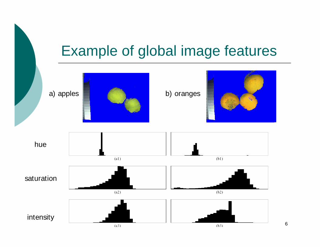
Example of global image features
a) apples b) oranges
hue
saturation
intensity
7
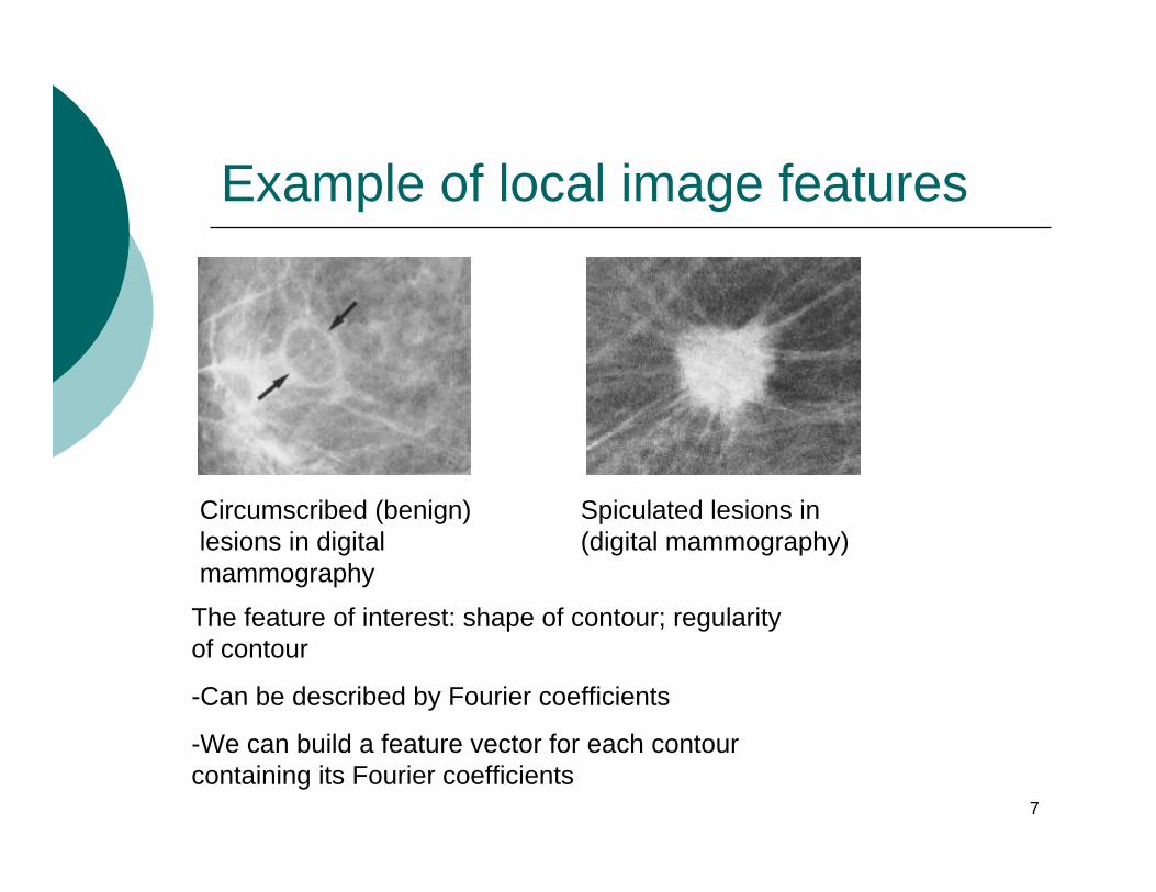
Example of local image features
Circumscribed (benign) lesions in digital mammography
Spiculated lesions in (digital mammography)
The feature of interest: shape of contour; regularity of contour
-Can be described by Fourier coefficients
-We can build a feature vector for each contour containing its Fourier coefficients
8
Image features
Are local, meaningful, detectable parts of an image:
Meaningful: features are associated to interesting scene elements in the image formation processThey should be invariant to some variations in the image formation process (i.e. invariance to viewpoint and illumination for images captured with digital cameras)
Detectable:They can be located/detected from images via algorithmsThey are described by a feature vector
9
Preprocessing
Pixel brightness transformations (also called gray scale transformations)
Do not depend on the position of the pixel in the image
Geometric transformationsModify both pixel coordinates and intensity levels
Neighborhood-based operations (filtering)
10
Outline
Rationale for image pre-processingGray-scale transformationsGeometric transformationsLocal preprocessing
Reading: Sonka et al 5.1, 5.2, 5.3
11
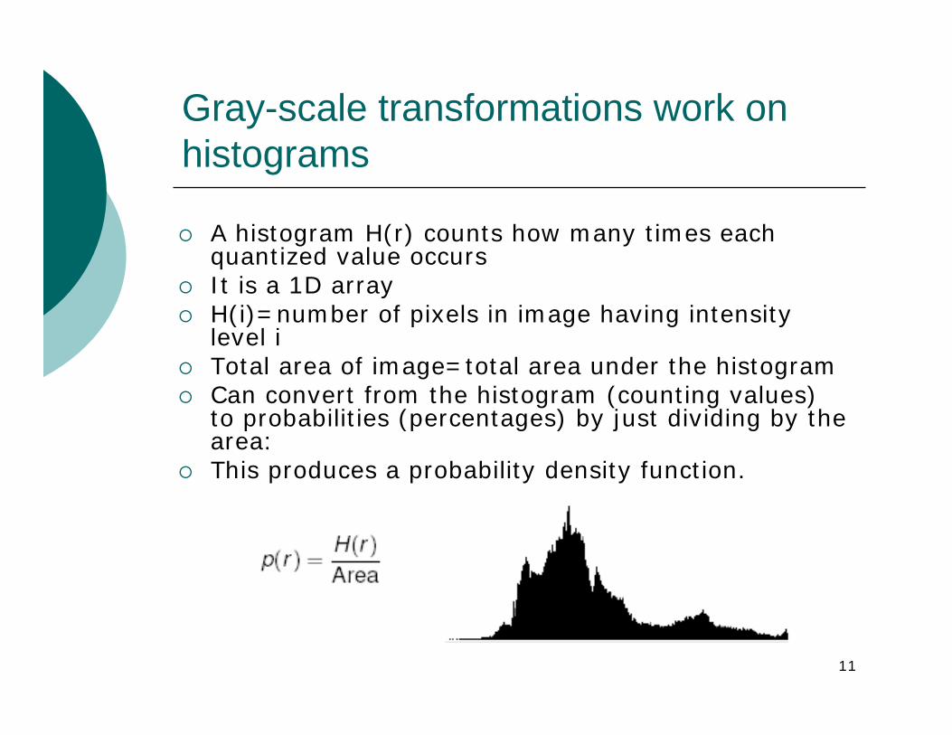
Gray-scale transformations work on histograms
A histogram H(r) counts how many times each quantized value occursIt is a 1D arrayH(i)=number of pixels in image having intensity level i Total area of image=total area under the histogramCan convert from the histogram (counting values) to probabilities (percentages) by just dividing by the area:This produces a probability density function.
12
Contrast adjustment on histograms
Adjusting constrast causes the histogram to stretch or shrink horizontally:
Stretching = more contrastShrinking = less contrast
13
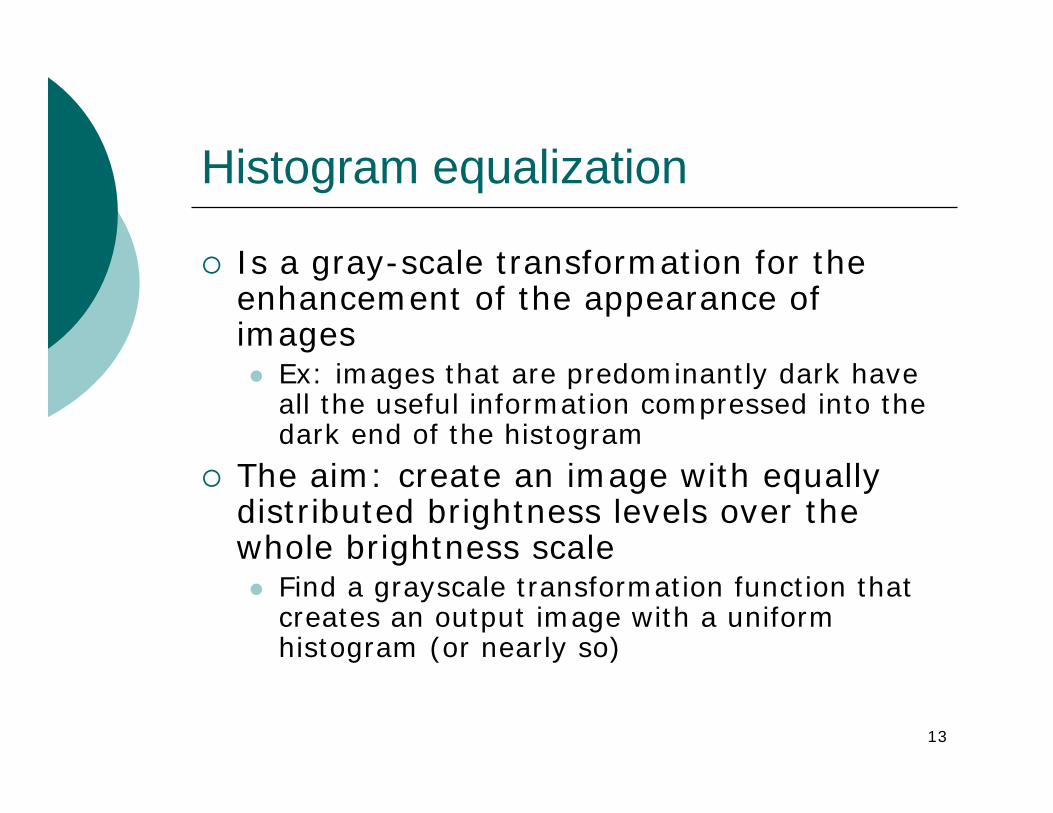
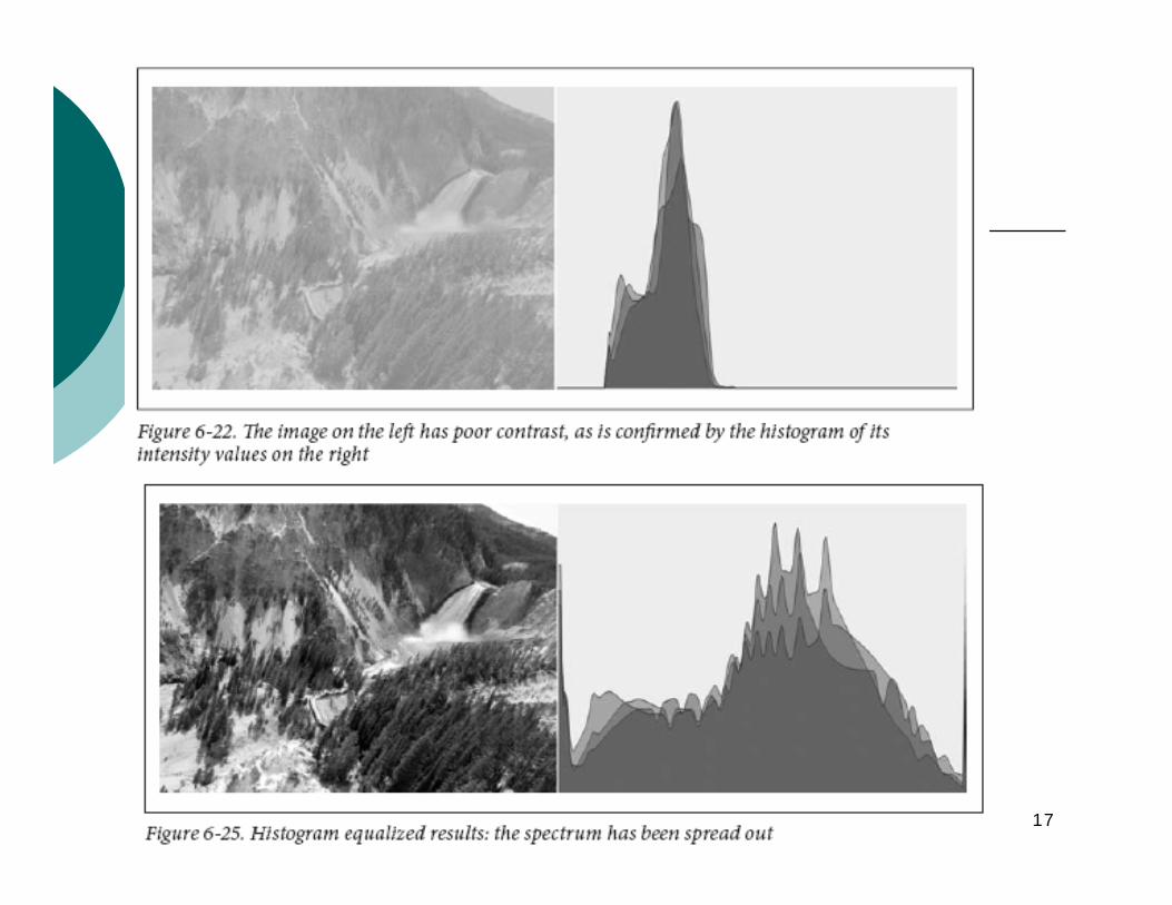
Histogram equalization
Is a gray-scale transformation for the enhancement of the appearance of images
Ex: images that are predominantly dark have all the useful information compressed into the dark end of the histogram
The aim: create an image with equally distributed brightness levels over the whole brightness scale
Find a grayscale transformation function that creates an output image with a uniform histogram (or nearly so)
14
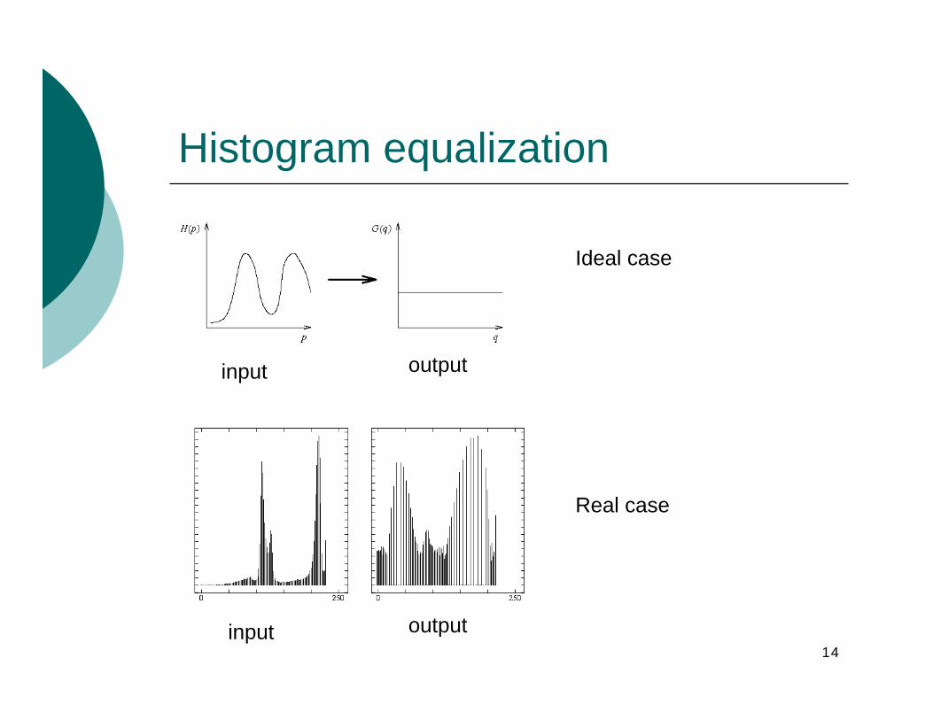
Histogram equalization
Ideal case
Real case
input output
input output
15
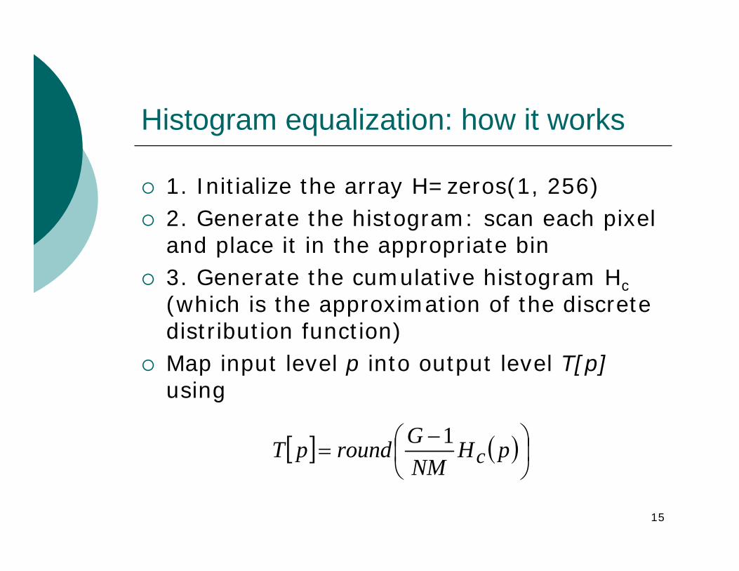
Histogram equalization: how it works
1. Initialize the array H=zeros(1, 256)2. Generate the histogram: scan each pixel and place it in the appropriate bin3. Generate the cumulative histogram Hc(which is the approximation of the discrete distribution function)Map input level p into output level T[p]using
[ ] ( )⎟⎠⎞
⎜⎝⎛ −
= pHNMGroundpT c
1
16
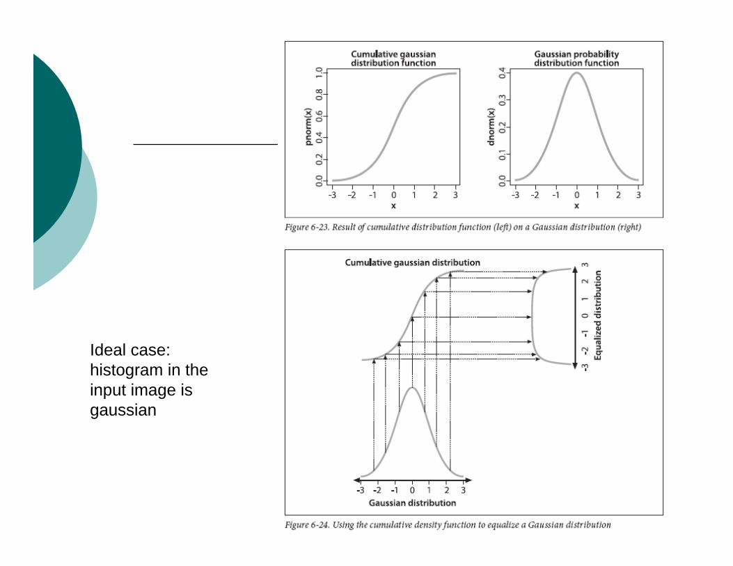
Ideal case: histogram in the input image is gaussian
17
Example
18
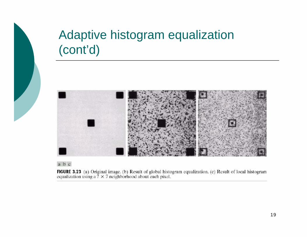
Adaptive histogram equalization
Allows localized contrast enhancement:ShadowsBackground variationsOther situations where global enhancement wouldn’t work
Remap based on local, not global histogramExample: 7x7 window around the point
Problem: ringing artifacts
19
Adaptive histogram equalization (cont’d)
20
Histogram specification
Histogram equalization: uniform output histogramWe can instead make it whatever we want it to be
Comparing two images“Stitching” multiple imagesImage-compositing operations
Use histogram equalization as an intermediate step
21
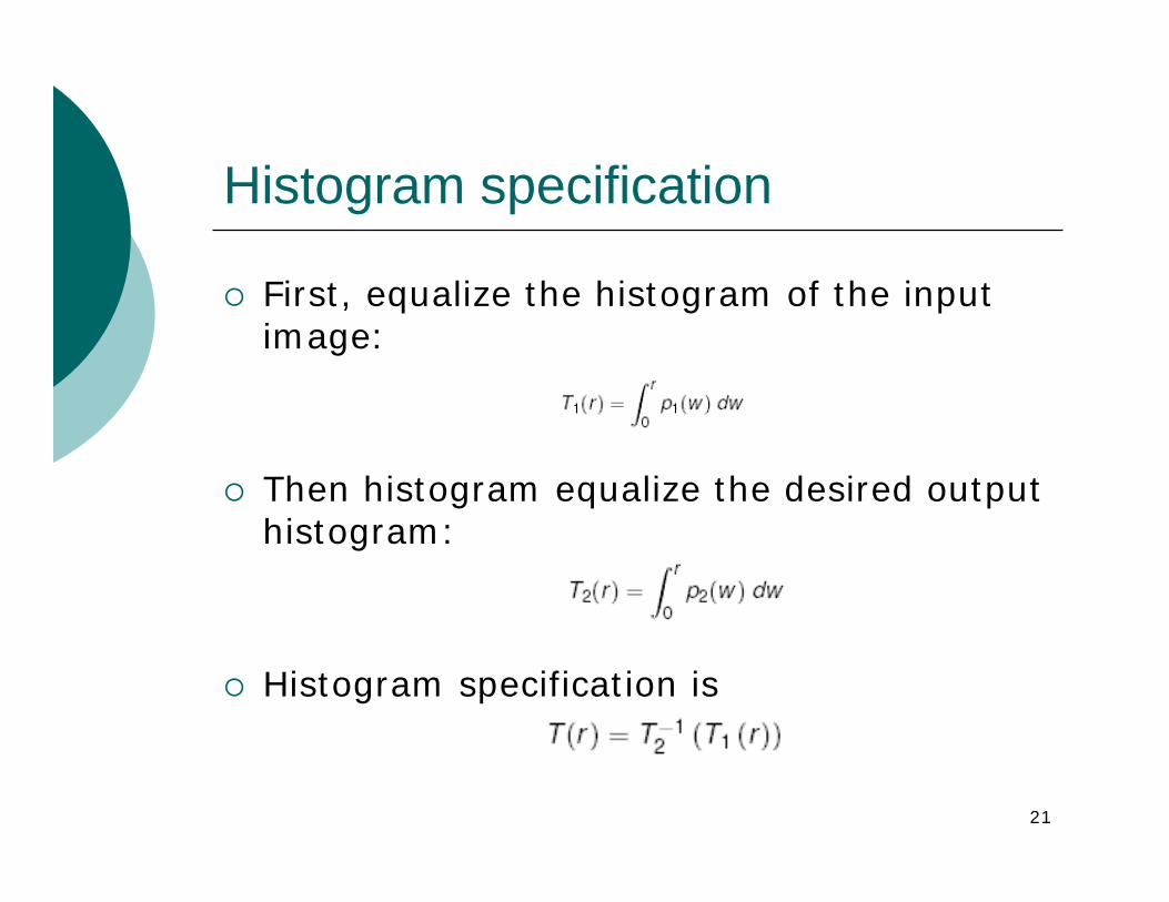
Histogram specification
First, equalize the histogram of the input image:
Then histogram equalize the desired output histogram:
Histogram specification is
22
Outline
Rationale for image pre-processingGray-scale transformationsGeometric transformationsLocal preprocessing
Reading: Sonka et al 5.1, 5.2, 5.3
23
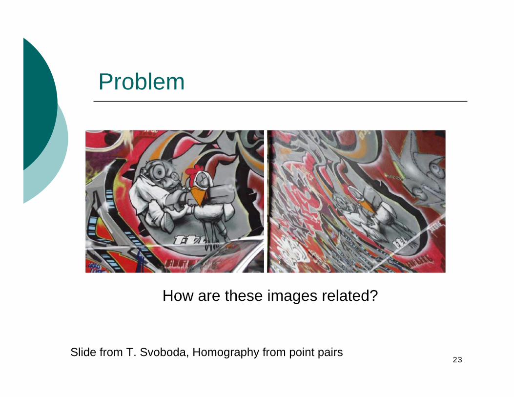
Problem
How are these images related?
Slide from T. Svoboda, Homography from point pairs
24
Geometric transformations
Commonly used in computer graphicsUsed in image analysis as well
Eliminate geometric distortion that occurs during image acquisitionUseful, for instance, when matching two or several images that correspond to the same object
Two basic steps:Pixel coordinate transformationBrightness interpolation
25
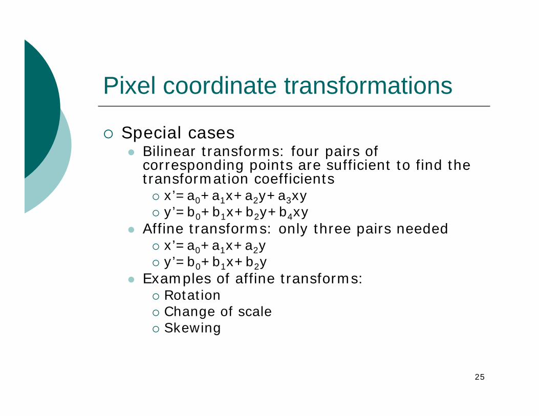
Pixel coordinate transformations
Special casesBilinear transforms: four pairs of corresponding points are sufficient to find the transformation coefficients
x’=a0+a1x+a2y+a3xyy’=b0+b1x+b2y+b4xy
Affine transforms: only three pairs neededx’=a0+a1x+a2yy’=b0+b1x+b2y
Examples of affine transforms:RotationChange of scaleSkewing
26
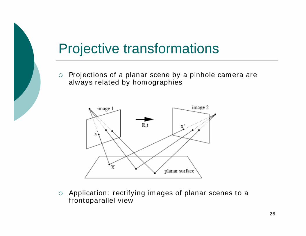
Projective transformations
Projections of a planar scene by a pinhole camera are always related by homographies
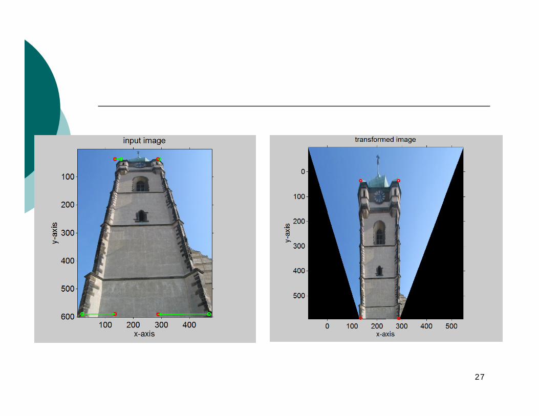
Application: rectifying images of planar scenes to a frontoparallel view
27
28
Outline
Rationale for image pre-processingGray-scale transformationsGeometric transformationsLocal preprocessing
Reading: Sonka et al 5.1, 5.2, 5.3
29
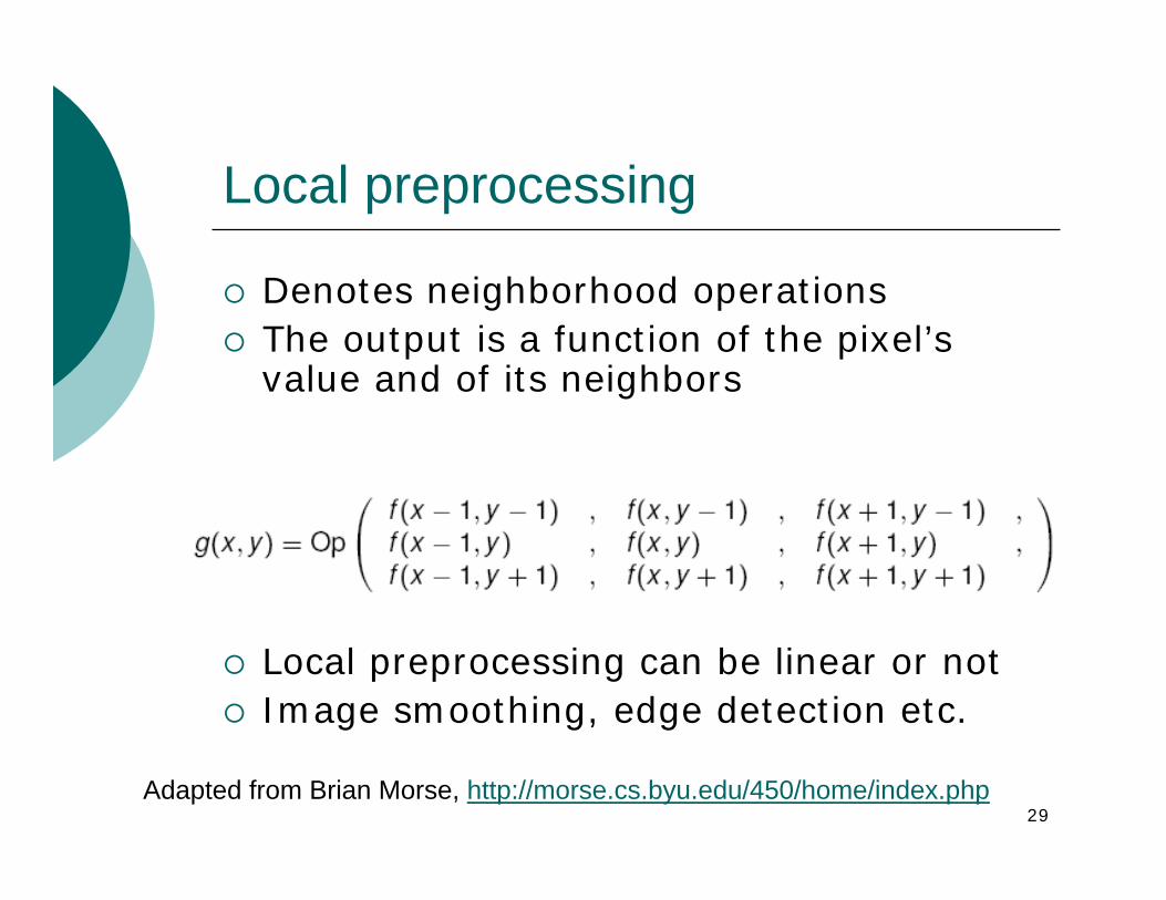
Local preprocessing
Denotes neighborhood operationsThe output is a function of the pixel’s value and of its neighbors
Weighted sums, average, min, max, median etcLocal preprocessing can be linear or notImage smoothing, edge detection etc.
Adapted from Brian Morse, http://morse.cs.byu.edu/450/home/index.php
30
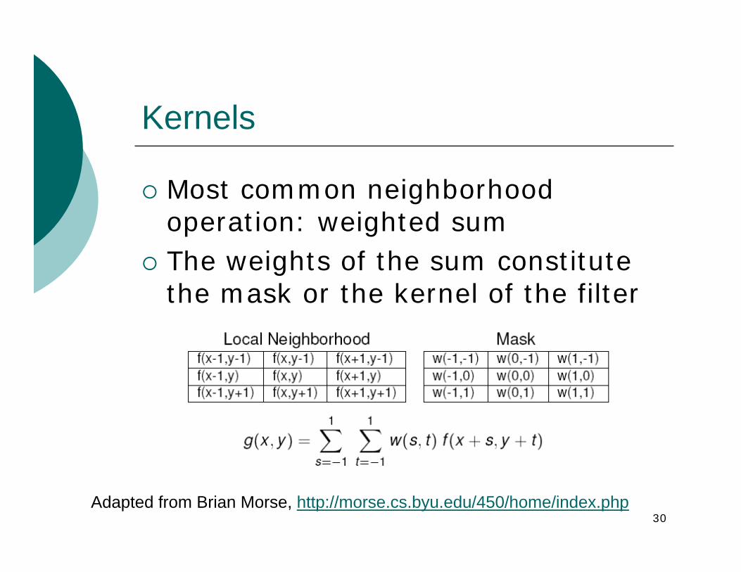
Kernels
Most common neighborhood operation: weighted sumThe weights of the sum constitute the mask or the kernel of the filter
Adapted from Brian Morse, http://morse.cs.byu.edu/450/home/index.php
31
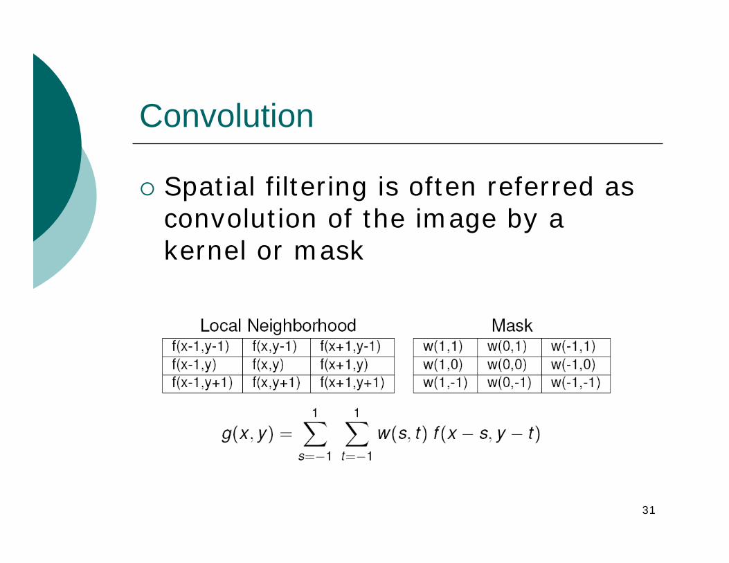
Convolution
Spatial filtering is often referred as convolution of the image by a kernel or mask
32
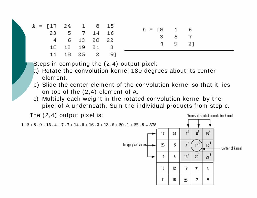
Steps in computing the (2,4) output pixel:a) Rotate the convolution kernel 180 degrees about its center
element. b) Slide the center element of the convolution kernel so that it lies
on top of the (2,4) element of A. c) Multiply each weight in the rotated convolution kernel by the
pixel of A underneath. Sum the individual products from step c.
The (2,4) output pixel is:
33
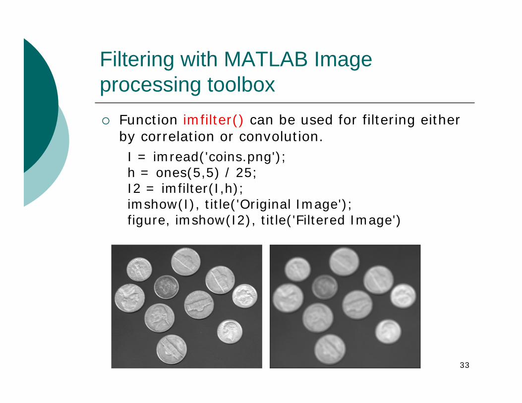
Filtering with MATLAB Image processing toolbox
Function imfilter() can be used for filtering either by correlation or convolution.I = imread('coins.png');h = ones(5,5) / 25;I2 = imfilter(I,h);imshow(I), title('Original Image');figure, imshow(I2), title('Filtered Image')
34
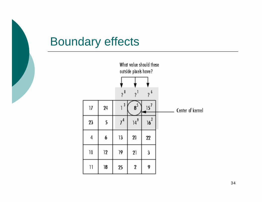
Boundary effects
35
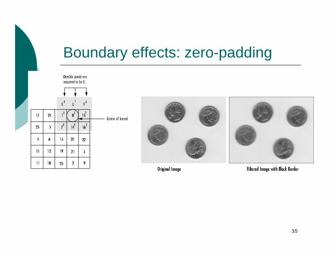
Boundary effects: zero-padding
36
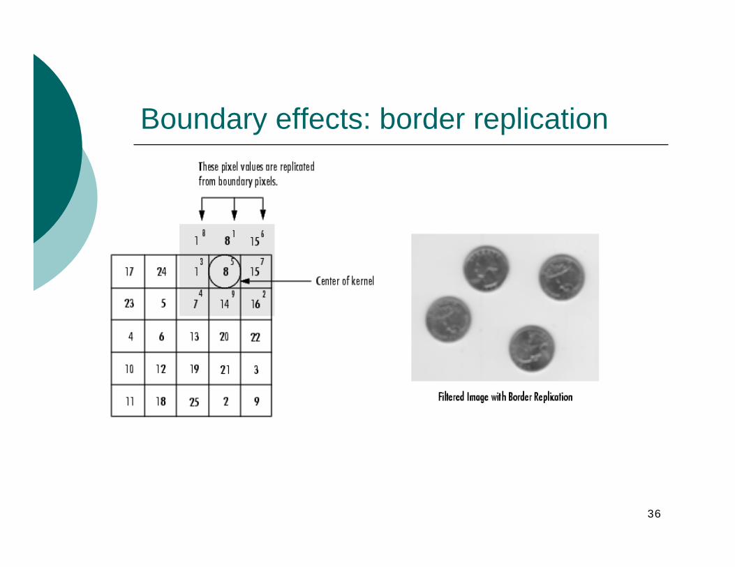
Boundary effects: border replication
37
Linear filtering for noise removal
What is noise?In computer vision, noise may refer to any entity, in images, data, or intermediate results, that is not interesting for the purposes of the main computationFor instance:
In edge detection algorithms, noise can be the spurious fluctuations of pixel values introduced by the image acquisition systemFor algorithms taking as input the results of some numerical computation, noise can be introduced by the computer’s limited precision, round-offs errors etc.We will concentrate on image noise
38
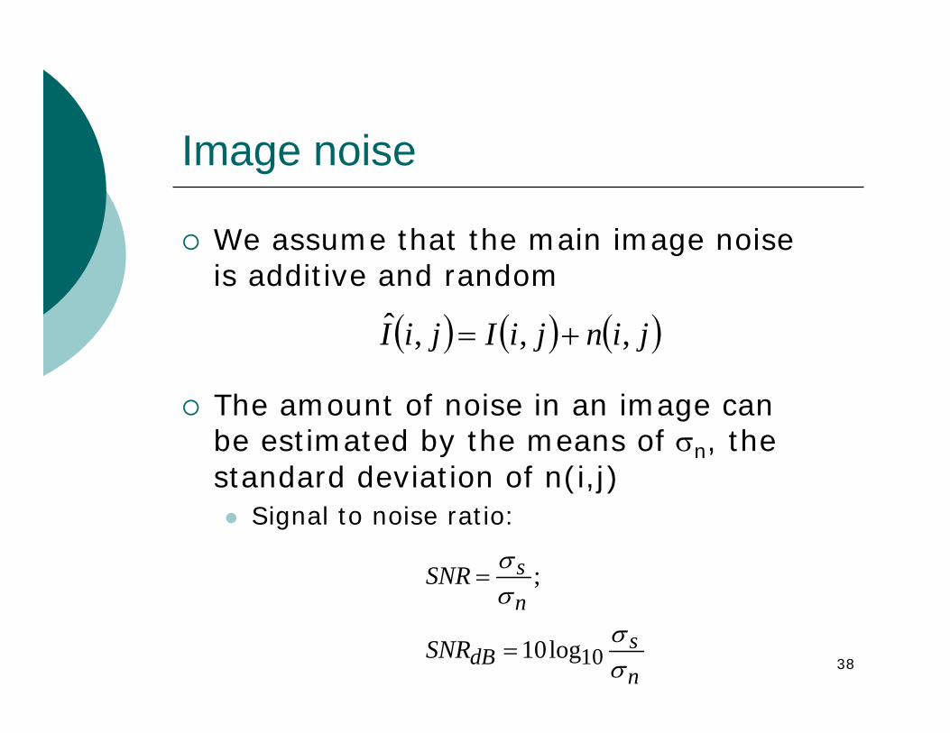
Image noise
We assume that the main image noise is additive and random
The amount of noise in an image can be estimated by the means of σn, the standard deviation of n(i,j)
Signal to noise ratio:
( ) ( ) ( )jinjiIjiI ,,,ˆ +=
ns
dB
ns
SNR
SNR
σσ
σσ
10log10
;
=
=
39
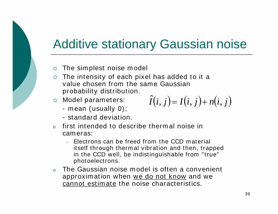
Additive stationary Gaussian noise
The simplest noise modelThe intensity of each pixel has added to it a value chosen from the same Gaussian probability distribution. Model parameters: - mean (usually 0);- standard deviation.
o first intended to describe thermal noise in cameras:
o Electrons can be freed from the CCD material itself through thermal vibration and then, trapped in the CCD well, be indistinguishable from "true" photoelectrons.
o The Gaussian noise model is often a convenient approximation when we do not know and we cannot estimate the noise characteristics.
( ) ( ) ( )jinjiIjiI ,,,ˆ +=
40
Limitations of stationary Gaussian noise
this model allows noise values that could be greater than maximum camera output or less than 0. Functions well only for small standard deviationsmay not be stationary (e.g. thermal gradients in the ccd)
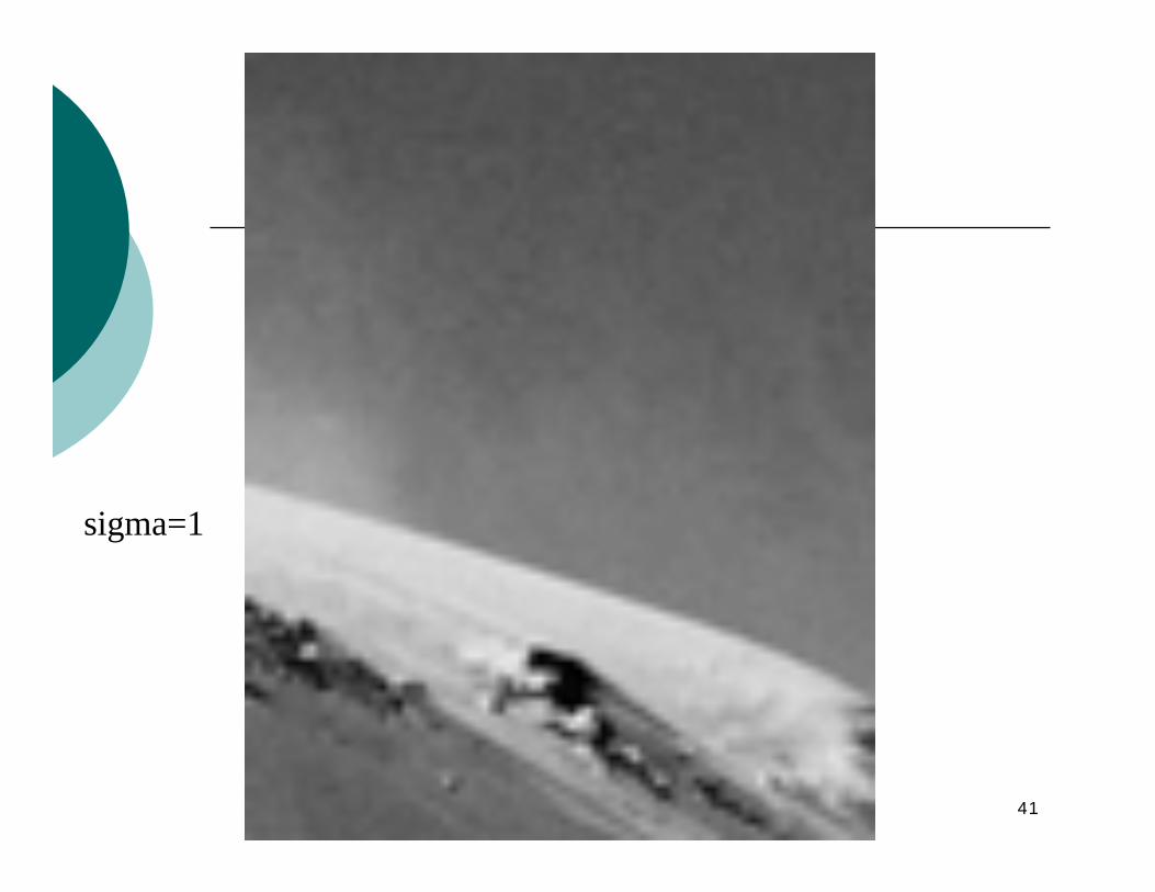
41
sigma=1
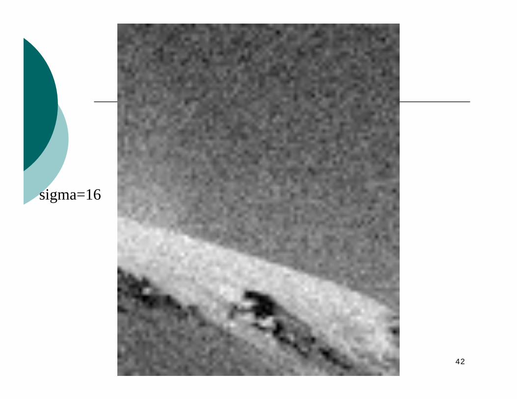
42
sigma=16
43
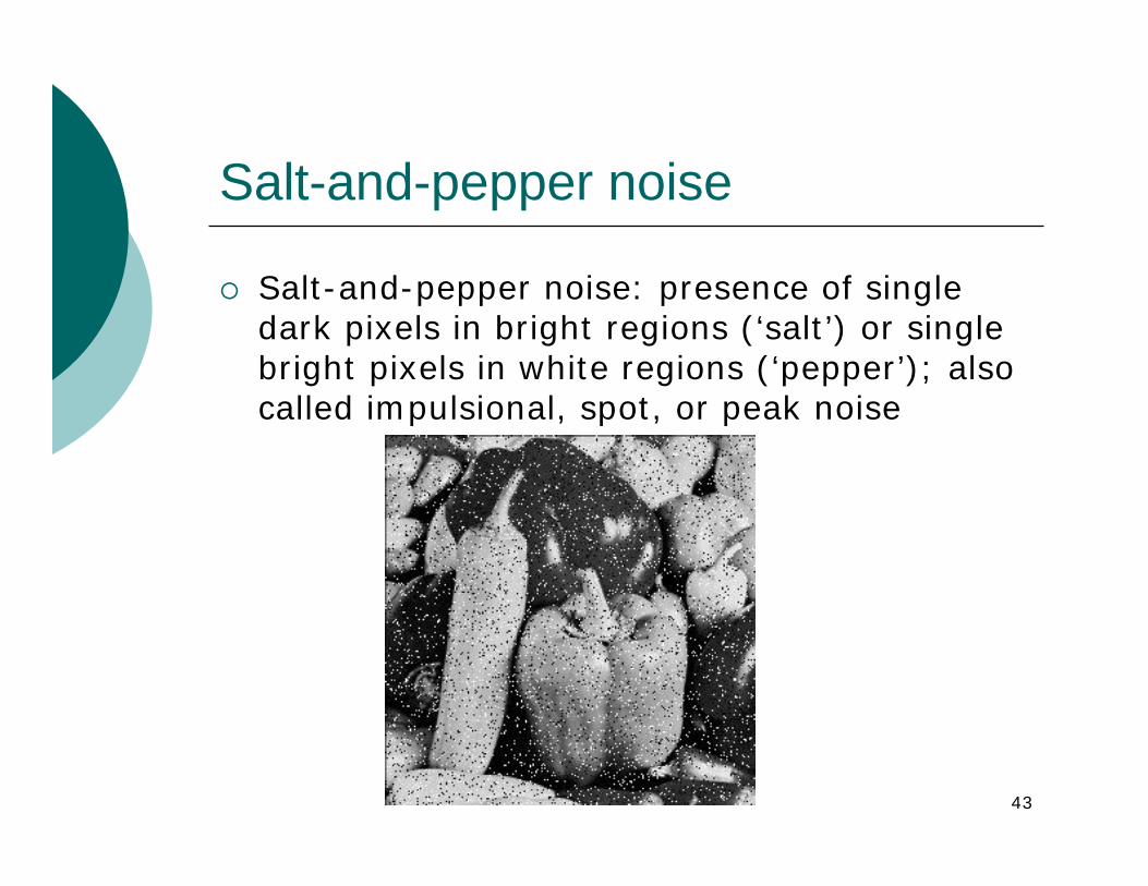
Salt-and-pepper noise
Salt-and-pepper noise: presence of single dark pixels in bright regions (‘salt’) or single bright pixels in white regions (‘pepper’); also called impulsional, spot, or peak noise
44
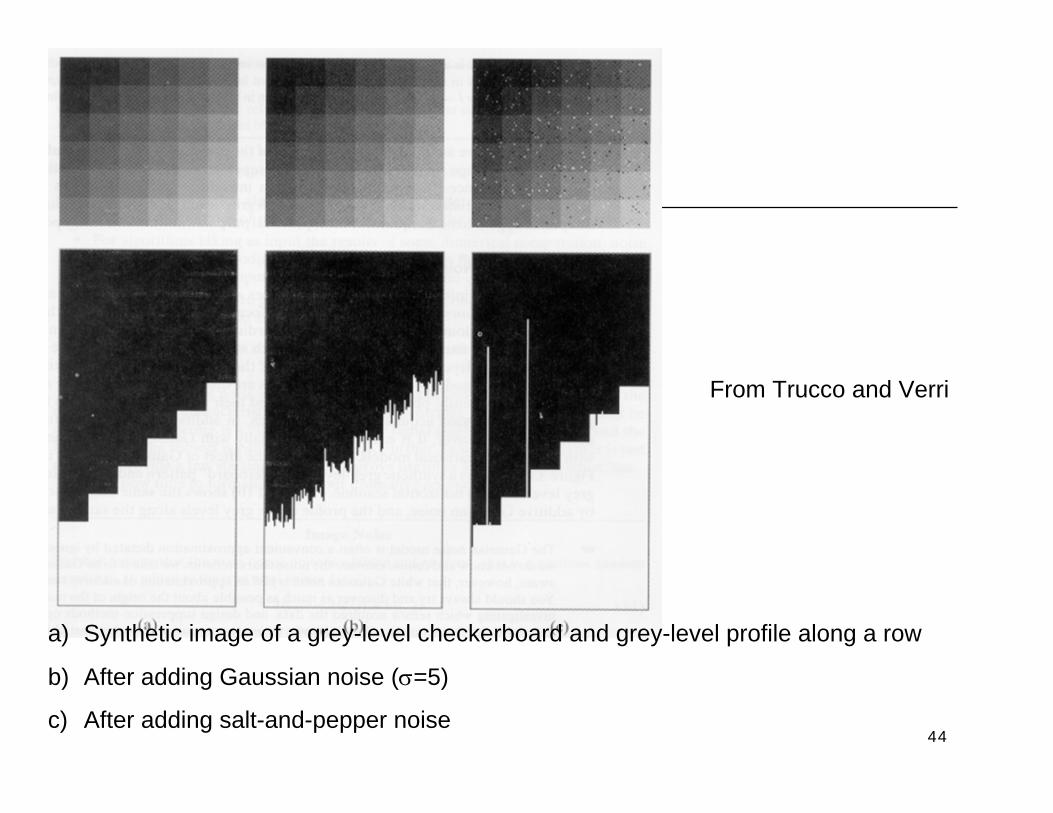
a) Synthetic image of a grey-level checkerboard and grey-level profile along a row
b) After adding Gaussian noise (σ=5)
c) After adding salt-and-pepper noise
From Trucco and Verri
45
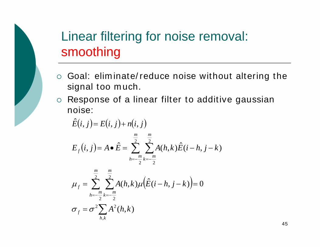
Linear filtering for noise removal: smoothing
Goal: eliminate/reduce noise without altering the signal too much.Response of a linear filter to additive gaussiannoise:
( ) ( ) ( )
( )
( )
∑
∑ ∑
∑ ∑
=
=−−=
−−=•=
+=
−= −=
−= −=
khf
m
mh
m
mk
f
m
mh
m
mk
f
khA
kjhiEkhA
kjhiEkhAEAjiE
jinjiEjiE
,
22
2
2
2
2
2
2
2
2
),(
0),(ˆ),(
),(ˆ),(ˆ,
,,,ˆ
σσ
μμ
46
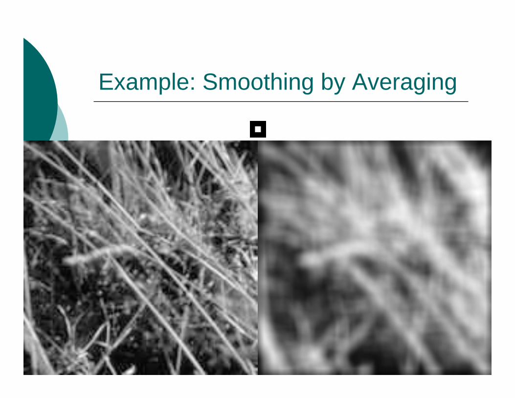
Example: Smoothing by Averaging
47
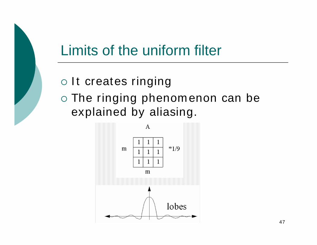
Limits of the uniform filter
It creates ringingThe ringing phenomenon can be explained by aliasing.
48
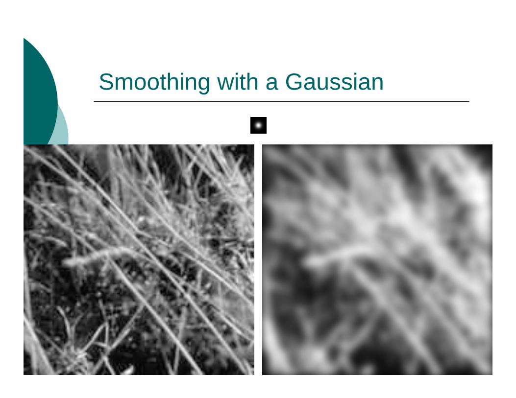
Smoothing with a Gaussian
49
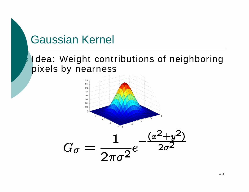
Gaussian KernelIdea: Weight contributions of neighboring pixels by nearness
50
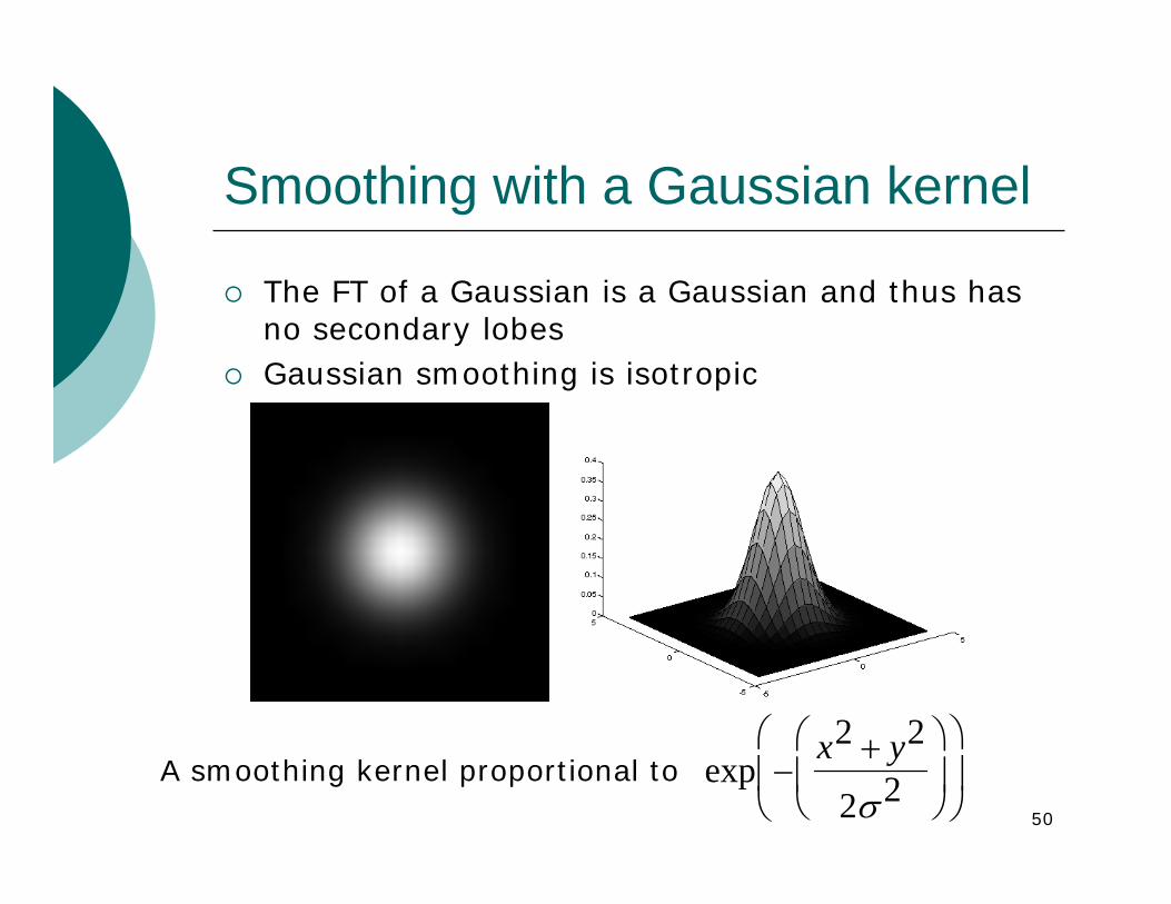
Smoothing with a Gaussian kernel
The FT of a Gaussian is a Gaussian and thus has no secondary lobesGaussian smoothing is isotropic
exp −x2 + y2
2σ 2⎛
⎝ ⎜
⎞
⎠ ⎟
⎛
⎝ ⎜
⎞
⎠ ⎟ A smoothing kernel proportional to
51
Design of a Gaussian filter
we need to produce a discrete approximation to the Gaussian function before we can perform the convolution. In theory, the Gaussian distribution is non-zero everywhere, which would require an infinitely large convolution mask.in practice it is effectively zero more than about three standard deviations from the mean, and so we can truncate the mask. The size of the mask is chosen according to σ.
w= 3Xσ
52
Gaussian filtering
Theorem of central limit: repeated convolution of a uniform 3X3 mask with itself yields a Gaussian filter.This is also called Gaussian smoothing by repeated averaging (RA)
Convolving a 3x3 mask n times with an image I approximates the Gaussian convolution of I with a Gaussian mask of
and size 3(n+1)-n=2n+3
3/n=σ
53
Smoothing with non-linear filters
Main problems of the averaging filter:1) Ringing introduces additional noise2) Impulsive noise is only attenuated and
diffused, not removed3) Sharp boundaries of objects are blurred.
Blurring will affect the accuracy of boundary detection
Note: first problem is solved by Gaussian filtersSecond and third problems are addressed by
non-linear filters (i.e. filters that can not be modeled as a convolution)
54
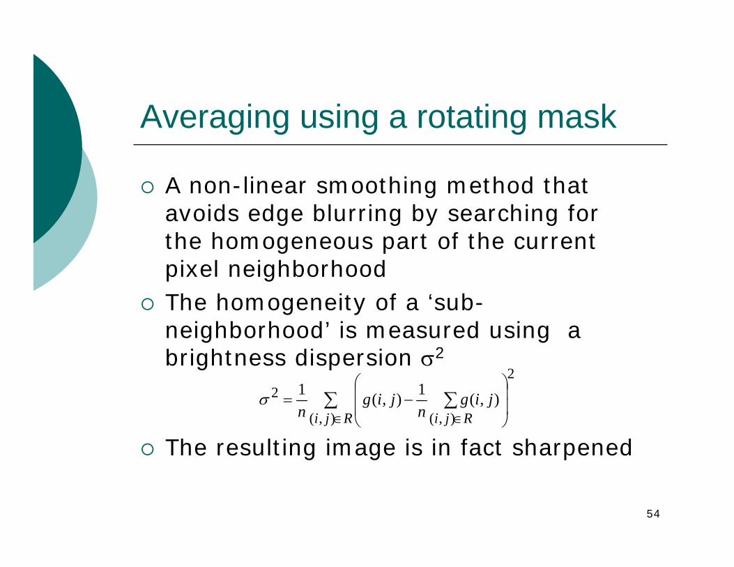
Averaging using a rotating mask
A non-linear smoothing method that avoids edge blurring by searching for the homogeneous part of the current pixel neighborhoodThe homogeneity of a ‘sub-neighborhood’ is measured using a brightness dispersion σ2
The resulting image is in fact sharpened
2
),( ),(
2 ),(1),(1∑ ∑
∈ ∈⎟⎟
⎠
⎞
⎜⎜
⎝
⎛−=
Rji Rjijig
njig
nσ
55
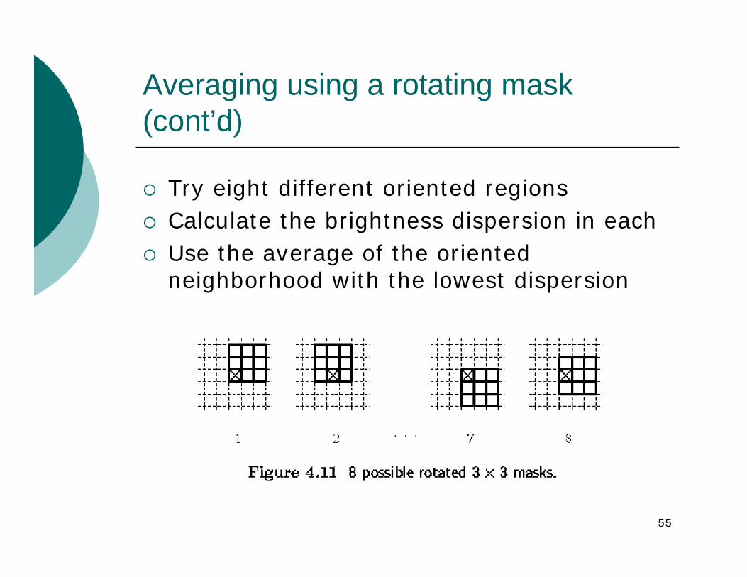
Averaging using a rotating mask (cont’d)
Try eight different oriented regionsCalculate the brightness dispersion in eachUse the average of the oriented neighborhood with the lowest dispersion
56
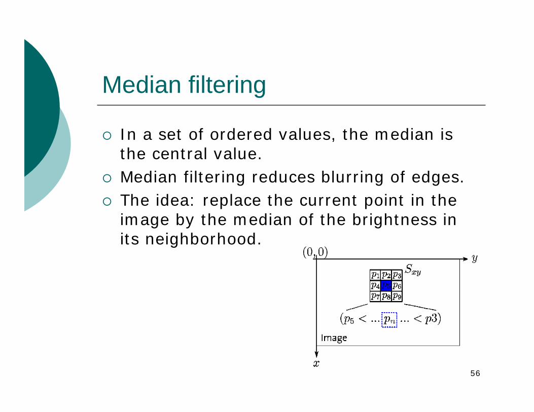
Median filtering
In a set of ordered values, the median is the central value. Median filtering reduces blurring of edges. The idea: replace the current point in the image by the median of the brightness in its neighborhood.
57
Median filtering: discussion
is not affected by individual noise spikes eliminates impulsive noise quite well does not blur edges much and can be applied iteratively.
Main disadvantage of median filtering in a rectangular neighborhood: damaging of thin lines and sharp corners in the image


