28
Week 2 - Sampling ESE 250 S'13 – Kod, DeHon & Kadric 1 ESE250: Digital Audio Basics Week 2 January 22, 2013 Sampling
| Date post: | 03-Jan-2016 |
| Category: |
Documents |
| Upload: | bertram-richards |
| View: | 229 times |
| Download: | 0 times |
Week 2 - Sampling 1ESE 250 S'13 – Kod, DeHon & Kadric
ESE250:Digital Audio Basics
Week 2 January 22, 2013
Sampling
Week 2 - Sampling 2
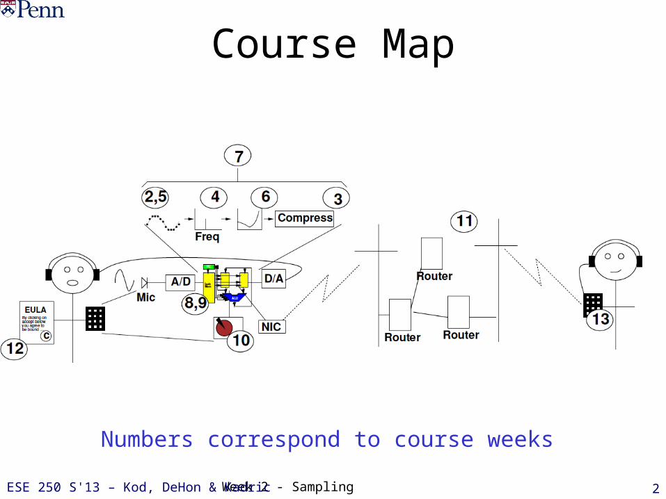
Course Map
Numbers correspond to course weeks
ESE 250 S'13 – Kod, DeHon & Kadric
Week 2 - Sampling 3
Digital Audio Agenda• Problem Statement
Given a limited set of resourceso memoryo computational power (instruction set, clock speed)
And a performance specification o What sort of errors o Are how damaging
Devise an audio signal recording and reconstruction architectureo that maximizes performanceo while remaining true to the resource constraints
• Agenda Weeks 2 – 7: explore the implications of finite (countable)
memory Weeks 8 - 11: exploit the capabilities of computational
engine
ESE 250 S'13 – Kod, DeHon & Kadric
Week 2 - Sampling 4
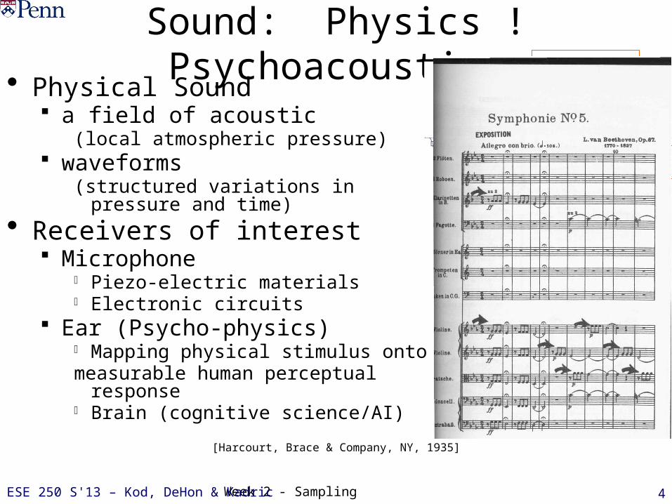
Sound: Physics ! Psychoacoustics
6 4 2 2 4 6
1.0
0.5
0.5
1.0
sec
? units
[Harcourt, Brace & Company, NY, 1935]
• Physical Sound a field of acoustic
(local atmospheric pressure) waveforms
(structured variations in pressure and time)• Receivers of interest
Microphone o Piezo-electric materialso Electronic circuits
Ear (Psycho-physics)o Mapping physical stimulus onto measurable human perceptual responseo Brain (cognitive science/AI)
ESE 250 S'13 – Kod, DeHon & Kadric
Week 2 - Sampling 5
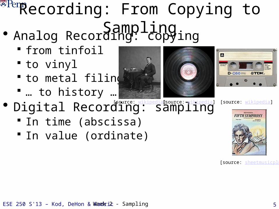
Recording: From Copying to Sampling• Analog Recording: copying
from tinfoil to vinyl to metal filings … to history …
• Digital Recording: sampling In time (abscissa) In value (ordinate)
[source: wikipedia] [source: wikipedia] [source: wikipedia]
[source: sheetmusicplus]
ESE 250 S'13 – Kod, DeHon & Kadric
Week 2 - Sampling 6
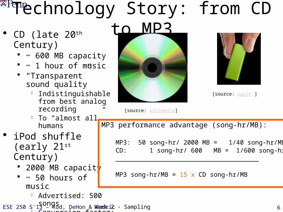
Technology Story: from CD to MP3• CD (late 20th Century)
~ 600 MB capacity ~ 1 hour of music “Transparent” sound
qualityo Indistinguishable from
best analog recordingo To “almost all” humans
• iPod shuffle (early 21st Century) 2000 MB capacity ~ 50 hours of music
o Advertised: 500 songso Conversion factor: ~ 6
min/song “Transparent” sound
quality
[source: wikipedia]
[source: apple ]
MP3 performance advantage (song-hr/MB):
MP3: 50 song-hr/ 2000 MB = 1/40 song-hr/MBCD: 1 song-hr/ 600 MB = 1/600 song-hr/MB______________________________________
MP3 song-hr/MB = 15 x CD song-hr/MB
ESE 250 S'13 – Kod, DeHon & Kadric
Week 2 - Sampling 7
What Changed?• Question(s) for this semester:
How does computation yield a net storage advantage? What other advantages does computation confer ?
• Question for this week’s lecture: (Baseline of technology story) How is sound represented and stored on a CD? Overview Answer:
o CD recorders sample waveform in time every 1/44000 seco CD recorders sample waveform in value at 65536 distinct levels
• Follow-on Question: can we do better?
ESE 250 S'13 – Kod, DeHon & Kadric
Week 2 - Sampling 8
• Intuition we ought to get a pretty good impression of a waveform’s
sound by dense sampling in time
• (some) Questions What do we mean by “impression”? What do we mean by “dense”? Doesn’t the answer depend upon the particular waveform? What else does it depend upon?
• (some) Answers: week 5
Quantizing in Time
ESE 250 S'13 – Kod, DeHon & Kadric
Week 2 - SamplingPenn ESE 250 S'12 - Kod & DeHon
Out[153]= 6 4 2 2 4 6
1.0
0.5
0.5
1.0
sec
volts
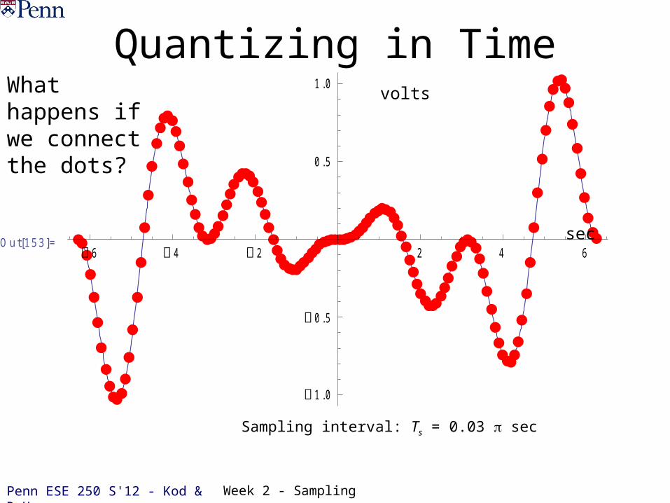
Sampling interval: Ts = 0.03 sec
Quantizing in TimeWhat happens if we connect the dots?

Week 2 - SamplingPenn ESE 250 S'12 - Kod & DeHon
Out[155]= 6 4 2 2 4 6
1.0
0.5
0.5
1.0
sec
volts
Sampling interval: Ts = 0.3 sec
Quantizing in TimeWhat happens if we connect the dots?
Week 2 - SamplingPenn ESE 250 S'12 - Kod & DeHon
Out[156]= 6 4 2 2 4 6
1.0
0.5
0.5
1.0
sec
volts
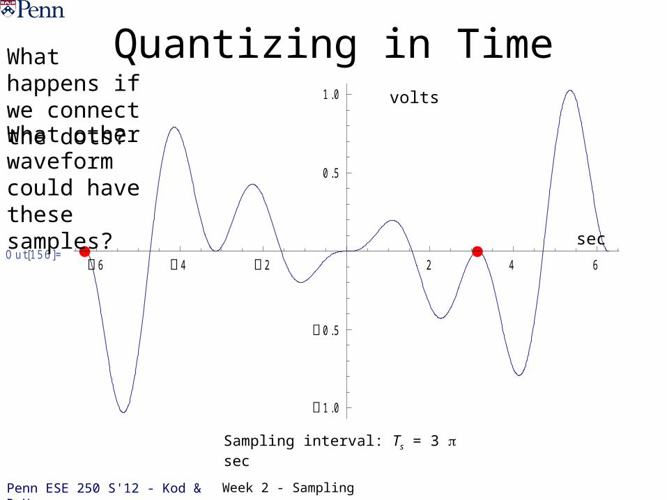
Sampling interval: Ts = 3 sec
Quantizing in TimeWhat happens if we connect the dots?What other waveform could have these samples?
Week 2 - SamplingPenn ESE 250 S'12 - Kod & DeHon
12
Out[168]= 6 4 2 2 4 6
1.0
0.5
0.5
1.0
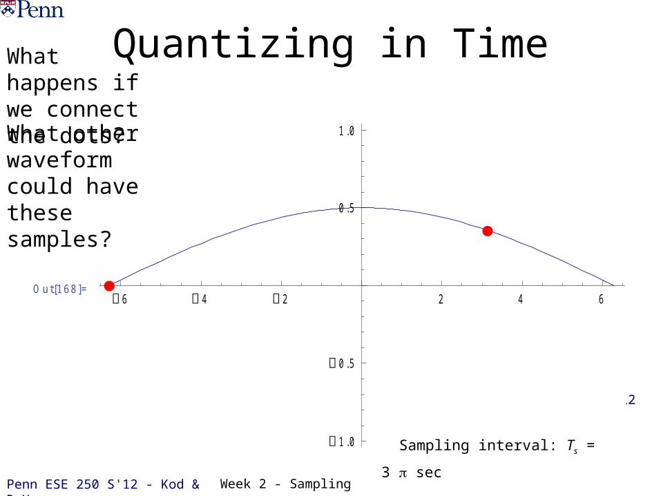
Sampling interval: Ts = 3 sec
Quantizing in TimeWhat happens if we connect the dots?What other waveform could have these samples?

Week 2 - Sampling 13
Quantizing in Value• Intuition
we ought to get a pretty good impression of a waveform’s sound by dense sampling of recorded voltage
• (some) Questions What do we mean by “impression”? What do we mean by “dense”? Doesn’t the answer depend upon the particular waveform? What else does it depend upon?
• (some) Answers: now + week 6
ESE 250 S'13 – Kod, DeHon & Kadric
Week 2 - Sampling 14
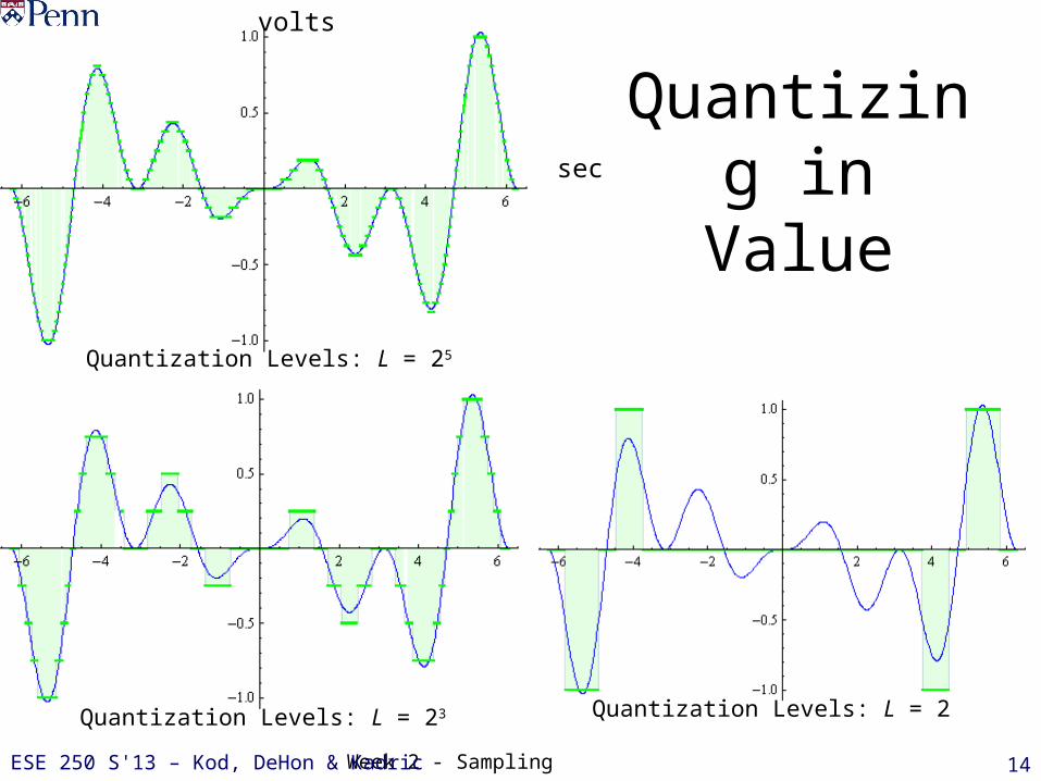
Quantizing in Value
sec
volts
Quantization Levels: L = 25
Quantization Levels: L = 23 Quantization Levels: L = 2
ESE 250 S'13 – Kod, DeHon & Kadric
Week 2 - Sampling 15
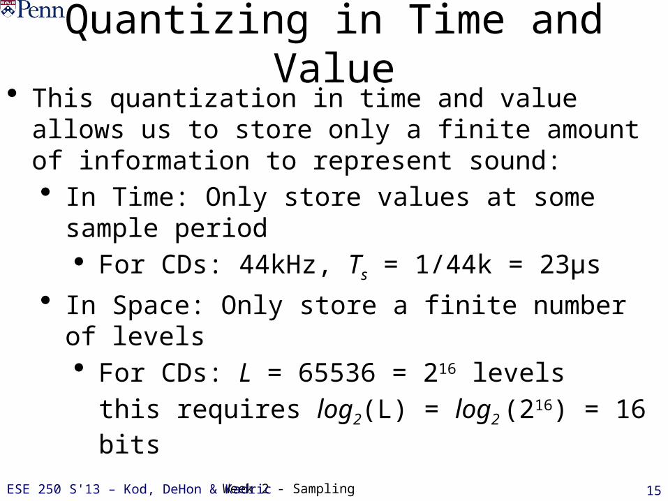
Quantizing in Time and Value• This quantization in time and value allows us to store
only a finite amount of information to represent sound:• In Time: Only store values at some sample period
• For CDs: 44kHz, Ts = 1/44k = 23μs
• In Space: Only store a finite number of levels• For CDs: L = 65536 = 216 levels
this requires log2(L) = log2 (216) = 16 bits
ESE 250 S'13 – Kod, DeHon & Kadric
Week 2 - Sampling
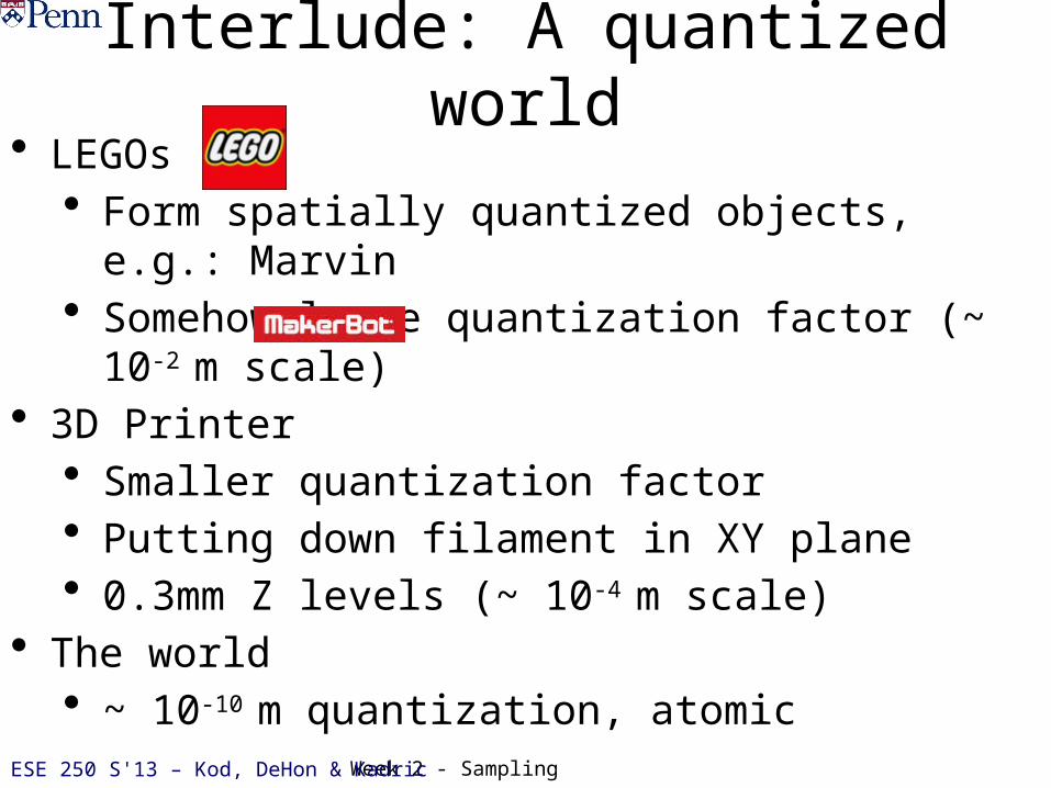
Interlude: A quantized world• LEGOs
• Form spatially quantized objects, e.g.: Marvin• Somehow large quantization factor (~ 10-2 m scale)
• 3D Printer • Smaller quantization factor• Putting down filament in XY plane• 0.3mm Z levels (~ 10-4 m scale)
• The world• ~ 10-10 m quantization, atomic
ESE 250 S'13 – Kod, DeHon & Kadric
Week 2 - Sampling 17
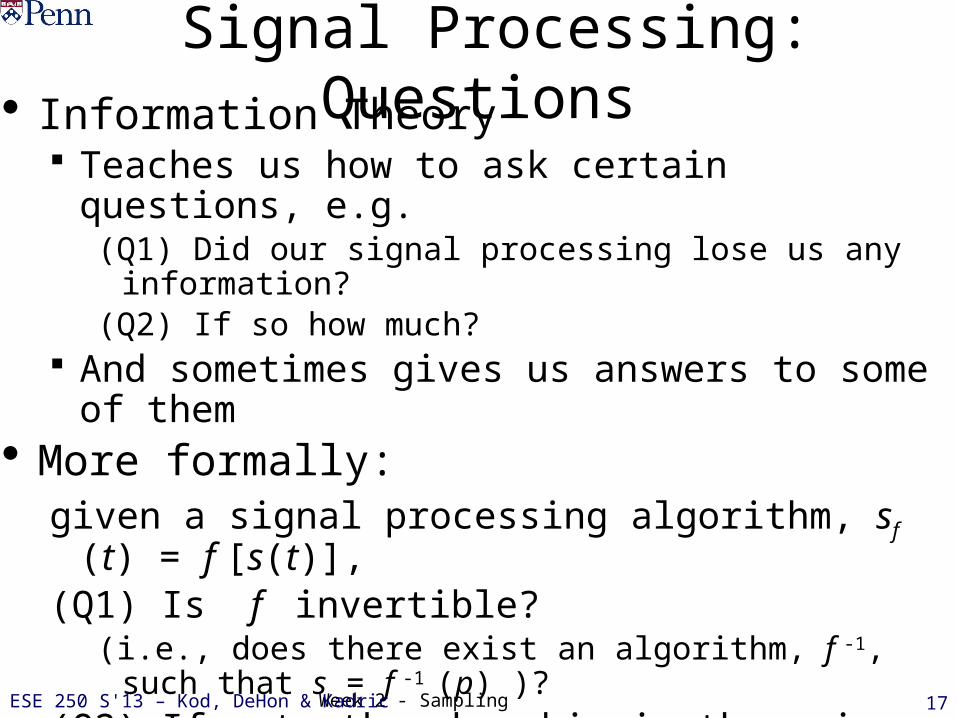
Signal Processing: Questions• Information Theory
Teaches us how to ask certain questions, e.g.(Q1) Did our signal processing lose us any information?(Q2) If so how much?
And sometimes gives us answers to some of them• More formally:
given a signal processing algorithm, sf (t) = f [s(t)], (Q1) Is f invertible?
(i.e., does there exist an algorithm, f -1, such that s = f -1 (p) )?
(Q2) If not, then how big is the noise, nf (s) = s – sf ?e.g.: invertible or not?
f(x) = x 2; g(x) = x 3; h(x) = sin(x)
ESE 250 S'13 – Kod, DeHon & Kadric
Week 2 - Sampling 18
2 1 1 2
2
1
1
2
2 1 1 2
2
1
1
2
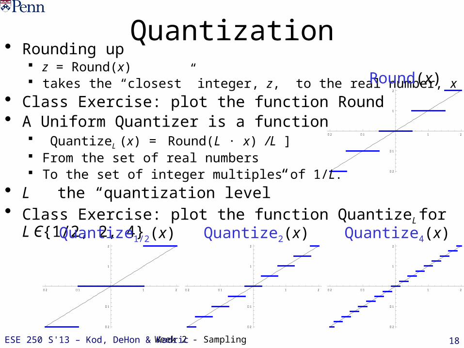
Quantization• Rounding up
z = Round(x) takes the “closest” integer, z, to the real number, x
• Class Exercise: plot the function Round• A Uniform Quantizer is a function
QuantizeL (x) = Round(L ∙ x) /L ] From the set of real numbers To the set of integer multiples of 1/L.
• L the “quantization level” • Class Exercise: plot the function QuantizeL for L Є{1/2, 2, 4}
2 1 1 2
2
1
1
2
2 1 1 2
2
1
1
2
Round(x)
Quantize1/2(x) Quantize2(x) Quantize4(x)
ESE 250 S'13 – Kod, DeHon & Kadric
Week 2 - Sampling 19
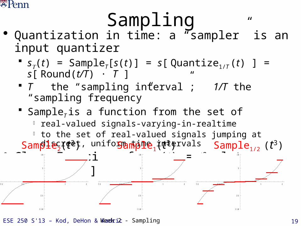
Sampling• Quantization in time: a “sampler” is an input quantizer
sT(t) = SampleT[s(t)] = s[ Quantize1/T (t) ] = s[ Round(t/T) ∙ T ] T the “sampling interval”; 1/T the “sampling frequency” SampleT is a function from the set of
o real-valued signals-varying-in-realtime o to the set of real-valued signals jumping at discreet, uniform time
intervals
• Class Exercise: for s(t) = t3 plot SampleT[s(t)], T 2 {1/2, 1, 2}
2 1 1 2
10
5
5
10
2 1 1 2
10
5
5
10
Sample2(t3) Sample1(t3)
2 1 1 2
10
5
5
10
Sample1/2 (t3)
ESE 250 S'13 – Kod, DeHon & Kadric
Week 2 - Sampling 20
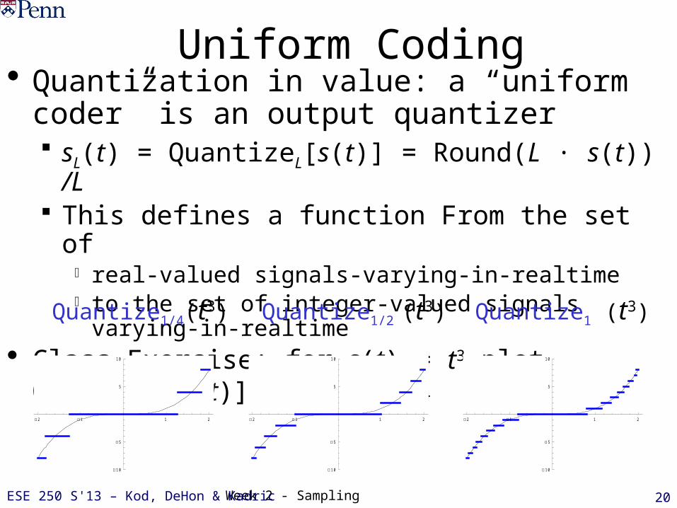
Uniform Coding• Quantization in value: a “uniform coder” is an
output quantizer sL(t) = QuantizeL[s(t)] = Round(L ∙ s(t)) /L This defines a function From the set of
o real-valued signals-varying-in-realtime o to the set of integer-valued signals varying-in-realtime
• Class Exercise: for s(t) = t3 plot QuantizeL[s(t)], L Є {1/4, 1/2, 1}
Quantize1/4(t3) Quantize1/2 (t3) Quantize1 (t3)
2 1 1 2
10
5
5
10
2 1 1 2
10
5
5
10
2 1 1 2
10
5
5
10
ESE 250 S'13 – Kod, DeHon & Kadric
Week 2 - Sampling 21
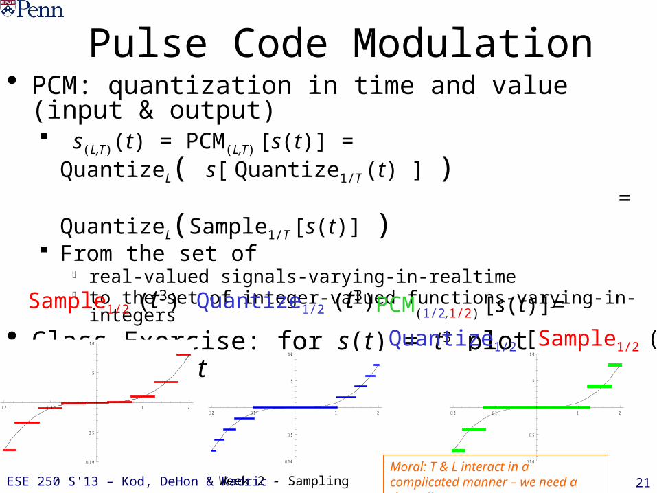
Pulse Code Modulation• PCM: quantization in time and value (input & output)
s(L,T)(t) = PCM(L,T) [s(t)] = QuantizeL( s[ Quantize1/T (t) ] ) = QuantizeL(Sample1/T [s(t)] ) From the set of
o real-valued signals-varying-in-realtime o to the set of integer-valued functions-varying-in-integers
• Class Exercise: for s(t) = t3 plot PCM(1/2,1/2) [s(t)]
Quantize1/2 (t3)
2 1 1 2
10
5
5
10
2 1 1 2
10
5
5
10
Sample1/2 (t3)
2 1 1 2
10
5
5
10
PCM(1/2,1/2) [s(t)]=
Quantize1/2 [Sample1/2 (t3)]
Moral: T & L interact in a complicated manner – we need a theory!!ESE 250 S'13 – Kod, DeHon & Kadric
Week 2 - Sampling 22
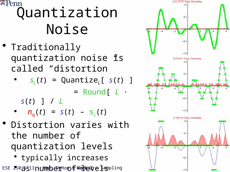
Quantization Noise
• Traditionally quantization noise is called “distortion” sL(t) = QuantizeL[ s(t) ]
= Round[ L ∙ s(t) ] / L nq(t) = s(t) – sL(t)
• Distortion varies with the number of quantization levels typically increases as number of levels decreases
ESE 250 S'13 – Kod, DeHon & Kadric
Week 2 - Sampling 23
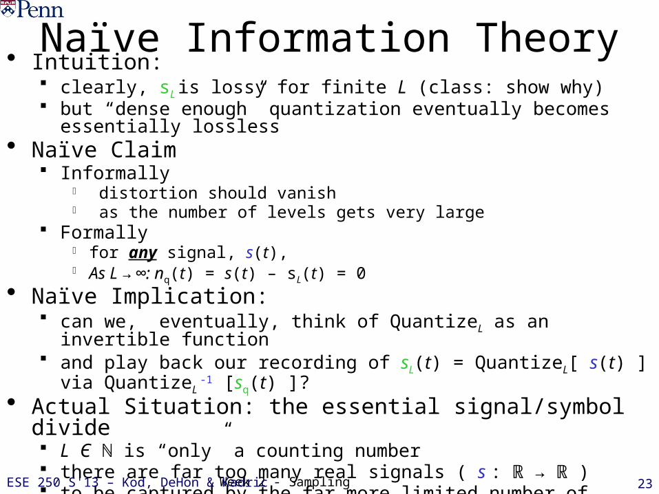
Naïve Information Theory• Intuition: clearly, sL is lossy for finite L (class: show why) but “dense enough” quantization eventually becomes essentially lossless
• Naïve Claim Informally
o distortion should vanish o as the number of levels gets very large
Formallyo for any signal, s(t), o As L → ∞: nq(t) = s(t) – sL(t) = 0
• Naïve Implication: can we, eventually, think of QuantizeL as an invertible function and play back our recording of sL(t) = QuantizeL[ s(t) ] via QuantizeL
-1 [sq(t) ]?• Actual Situation: the essential signal/symbol divide
L Є is “only” a counting numberℕ there are far too many real signals ( s : → )ℝ ℝ to be captured by the far more limited number of quantized signals, sL(t)
ESE 250 S'13 – Kod, DeHon & Kadric

Week 2 - Sampling 24
Toward a Model-Driven Theory• Why did we bother to try to represent all signals?
No physical source could produce some mathematically conceivable signals
No animal organ could transduce some physically plausible signals
No human listener could hear some perceptually active sounds
• Let’s assume-away the irrelevant The more we constrain the class of signals The more efficiently we will be able to process them
ESE 250 S'13 – Kod, DeHon & Kadric
Week 2 - Sampling 25
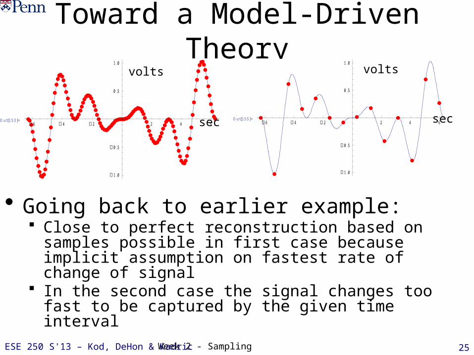
Toward a Model-Driven Theory
• Going back to earlier example: Close to perfect reconstruction based on samples possible in
first case because implicit assumption on fastest rate of change of signal
In the second case the signal changes too fast to be captured by the given time interval
ESE 250 S'13 – Kod, DeHon & Kadric
Out[153]= 6 4 2 2 4 6
1.0
0.5
0.5
1.0
sec
volts
Out[155]= 6 4 2 2 4 6
1.0
0.5
0.5
1.0
sec
volts
Week 2 - Sampling 26
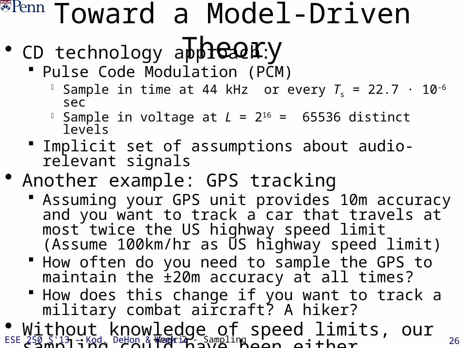
Toward a Model-Driven Theory• CD technology approach:
Pulse Code Modulation (PCM)o Sample in time at 44 kHz or every Ts = 22.7 · 10-6 seco Sample in voltage at L = 216 = 65536 distinct levels
Implicit set of assumptions about audio-relevant signals• Another example: GPS tracking
Assuming your GPS unit provides 10m accuracy and you want to track a car that travels at most twice the US highway speed limit (Assume 100km/hr as US highway speed limit)
How often do you need to sample the GPS to maintain the ±20m accuracy at all times?
How does this change if you want to track a military combat aircraft? A hiker?
• Without knowledge of speed limits, our sampling could have been either inaccurate or inefficient
ESE 250 S'13 – Kod, DeHon & Kadric

Week 2 - Sampling 27
Models: “generative” information • A “model”
is a set of (computationally expressed) assumptions about the sender and/or the receiver of any signal to be processed
• By thus delimiting the class of signals we achieve (in theory) the possibility of exact reconstruction (in practice) the ability to predict
o how quickly the processing noise will diminisho as our computational resources are increased
for the “cost” of o keeping around (and then executing in use) some “side information”o (a mathematical/computational representation of the model) o that is systematically used in reconstructing the signal from its stored record
• Examples: Audio processing: we will model the receiver (the human auditory
system) Speech processing: we add a model of the sender (the properties of
language)
ESE 250 S'13 – Kod, DeHon & Kadric
Week 2 - Sampling 28
ESE250:Digital Audio Basics
End Week 2 Lecture
Sampling
ESE 250 S'13 – Kod, DeHon & Kadric


