97
Week 5: Midterm revision session Jack Blumenau & Philipp Broniecki University College London Introduction to Quantitative Methods Week 5: Midterm revision session Introduction to QM 1 / 35

Week 5: Midterm revision session
Jack Blumenau & Philipp Broniecki
University College London
Introduction to Quantitative Methods
Week 5: Midterm revision session Introduction to QM 1 / 35

1 Administrative information
2 Answer advice
3 Hypothesis testing
4 Simple linear regression
5 Multiple linear regression
Week 5: Midterm revision session Introduction to QM 2 / 35

Overview
1 Administrative information
2 Answer advice
3 Hypothesis testing
4 Simple linear regression
5 Multiple linear regression
Week 5: Midterm revision session Administrative information Introduction to QM 3 / 35
Administrative information
• Midterm will be released at 2pm on November 3rd
• Midterm is due at 2pm on November 8th
• All submissions via Turnitin
• Usual late penalties apply
• Usual extenuating circumstances policies apply
Week 5: Midterm revision session Administrative information Introduction to QM 4 / 35

Overview
1 Administrative information
2 Answer advice
3 Hypothesis testing
4 Simple linear regression
5 Multiple linear regression
Week 5: Midterm revision session Answer advice Introduction to QM 5 / 35

How much detail do I need to include?
• You will not lose marks for writing fewer than 1000 words
• You will lose marks for writing more than 1000 words
• Your answer should include sufficient detail to fully answer thequestion
◦ Statistical information. e.g. How do we interpret theconfidence interval?
◦ Substantive information. e.g. What does this tell us aboutour research question?
Week 5: Midterm revision session Answer advice Introduction to QM 6 / 35
How should I present my answers?
• You need to write in full sentences, not bullet points
• You should present output of all statistical tests in a clear andreadable format
◦ Do not copy and paste output from R◦ Do not include screenshots from R◦ Use screenreg or make a table in Word
• Answer the question! If you are asked to answer a policyrelevant question, you should not simply report a p-valuewithout commenting on the substance.
• You can use R to answer any question where you think itmight be useful. But if the question tells you to ‘show yourwork’, that means you need to show that you know how thevalues from R were calculated!
Week 5: Midterm revision session Answer advice Introduction to QM 7 / 35

Overview
1 Administrative information
2 Answer advice
3 Hypothesis testing
4 Simple linear regression
5 Multiple linear regression
Week 5: Midterm revision session Hypothesis testing Introduction to QM 8 / 35

Intuition
• Could a relationship we observe in our data have happened bychance?
• What is the probability that there is no relationship eventhough we observed it in our sample?
1 Is the sample mean different from some hypothesised value?
2 Are the means in subgroups of our data different? E.g., isaverage income in Scotland different from income in Wales?
3 Is effect of some X variable on some Y variable different from0?
Week 5: Midterm revision session Hypothesis testing Introduction to QM 9 / 35

Hypothesis test sequence
• State the hypothesis and the null hypothesis
• Calculate a test-statistic
• Derive the sampling distribution of the test statistic under theassumption that the null hypothesis is true
• Calculate the p-value
• State a conclusion
Week 5: Midterm revision session Hypothesis testing Introduction to QM 10 / 35

Test for the sample mean: hypothesis
Is the die loadedEach outcome on a die is equally likely. Thus, the average outcomefrom throwing a fair die often is 3.5. If we take a die and throw it100 times and and get an average of 3.46, is that evidence for aloaded die or not?
• Null Hypothesis: die is fair. The small difference we find is dueto chance.
• Hypothesis: The die is loaded. The difference is systematic
Week 5: Midterm revision session Hypothesis testing Introduction to QM 11 / 35

Test for the sample mean: t value
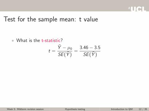
• What is the t-statistic?
t =Y − µ0
SE (Y )=
3.46− 3.5
SE (Y )
• The t-statistic is the difference in means. It’s units are averagedistances from the true mean (standard deviations).
• We do not know the standard deviation of the samplingdistribution, so we estimate it with the standard error
Week 5: Midterm revision session Hypothesis testing Introduction to QM 12 / 35

Test for the sample mean: t value
• What is the t-statistic?
t =Y − µ0
SE (Y )
=3.46− 3.5
SE (Y )
• The t-statistic is the difference in means. It’s units are averagedistances from the true mean (standard deviations).
• We do not know the standard deviation of the samplingdistribution, so we estimate it with the standard error
Week 5: Midterm revision session Hypothesis testing Introduction to QM 12 / 35
Test for the sample mean: t value
• What is the t-statistic?
t =Y − µ0
SE (Y )=
3.46− 3.5
SE (Y )
• The t-statistic is the difference in means. It’s units are averagedistances from the true mean (standard deviations).
• We do not know the standard deviation of the samplingdistribution, so we estimate it with the standard error
Week 5: Midterm revision session Hypothesis testing Introduction to QM 12 / 35

Test for the sample mean: t value
• What is the t-statistic?
t =Y − µ0
SE (Y )=
3.46− 3.5
SE (Y )
• The t-statistic is the difference in means. It’s units are averagedistances from the true mean (standard deviations).
• We do not know the standard deviation of the samplingdistribution, so we estimate it with the standard error
Week 5: Midterm revision session Hypothesis testing Introduction to QM 12 / 35
Test for the sample mean: t value (2)
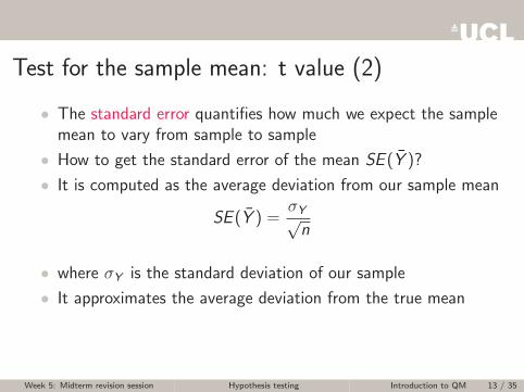
• The standard error quantifies how much we expect the samplemean to vary from sample to sample
• How to get the standard error of the mean SE (Y )?
• It is computed as the average deviation from our sample mean
SE (Y ) =σY√n
• where σY is the standard deviation of our sample
• It approximates the average deviation from the true mean
• Formally, it is an estimate for the standard deviation of thesampling distribution
Week 5: Midterm revision session Hypothesis testing Introduction to QM 13 / 35

Test for the sample mean: t value (2)
• The standard error quantifies how much we expect the samplemean to vary from sample to sample
• How to get the standard error of the mean SE (Y )?
• It is computed as the average deviation from our sample mean
SE (Y ) =σY√n
• where σY is the standard deviation of our sample
• It approximates the average deviation from the true mean
• Formally, it is an estimate for the standard deviation of thesampling distribution
Week 5: Midterm revision session Hypothesis testing Introduction to QM 13 / 35

Test for the sample mean: t value (3)
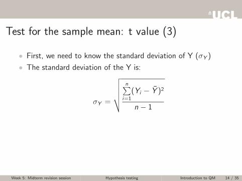
• First, we need to know the standard deviation of Y (σY )
• The standard deviation of the Y is:
σY =
√√√√√ n∑i=1
(Yi − Y )2
n − 1
• You cannot compute it from the information we have givenyou here. You would need to know all Yi values
• Suppose: σY = 1.69
Week 5: Midterm revision session Hypothesis testing Introduction to QM 14 / 35
Test for the sample mean: t value (3)
• First, we need to know the standard deviation of Y (σY )
• The standard deviation of the Y is:
σY =
√√√√√ n∑i=1
(Yi − Y )2
n − 1
• You cannot compute it from the information we have givenyou here. You would need to know all Yi values
• Suppose: σY = 1.69
Week 5: Midterm revision session Hypothesis testing Introduction to QM 14 / 35

Test for the sample mean: t value (4)
• We have all pieces to get the standard error of the meanSE (Y )
SE (Y )
=σY√n
=1.69√
100=
1.69
10= 0.17
Week 5: Midterm revision session Hypothesis testing Introduction to QM 15 / 35

Test for the sample mean: t value (4)
• We have all pieces to get the standard error of the meanSE (Y )
SE (Y ) =σY√n
=1.69√
100=
1.69
10= 0.17
Week 5: Midterm revision session Hypothesis testing Introduction to QM 15 / 35

Test for the sample mean: t value (4)
• We have all pieces to get the standard error of the meanSE (Y )
SE (Y ) =σY√n
=1.69√
100
=1.69
10= 0.17
Week 5: Midterm revision session Hypothesis testing Introduction to QM 15 / 35

Test for the sample mean: t value (4)
• We have all pieces to get the standard error of the meanSE (Y )
SE (Y ) =σY√n
=1.69√
100=
1.69
10
= 0.17
Week 5: Midterm revision session Hypothesis testing Introduction to QM 15 / 35

Test for the sample mean: t value (4)
• We have all pieces to get the standard error of the meanSE (Y )
SE (Y ) =σY√n
=1.69√
100=
1.69
10= 0.17
Week 5: Midterm revision session Hypothesis testing Introduction to QM 15 / 35
Test for the sample mean: t value (5)
• Now we can calculate t
t =Y − µ0
SE (Y )
=3.46− 3.5
SE (Y )=
3.46− 3.5
0.17=−0.04
0.17= −0.24
• The difference between our observed mean & the null is -0.24average deviations (standard errors) from the true mean.
• That’s not much! Our sample is large, so if we repeated ourtrial 100 times:
◦ 68 sample means will be within 1 standard error of true mean◦ 95 would be within 1.96 standard errors of the true mean
• We therefore know that the null is not that unlikely → We failto reject the null hypothesis
Week 5: Midterm revision session Hypothesis testing Introduction to QM 16 / 35

Test for the sample mean: t value (5)
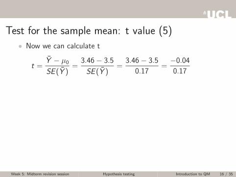
• Now we can calculate t
t =Y − µ0
SE (Y )=
3.46− 3.5
SE (Y )
=3.46− 3.5
0.17=−0.04
0.17= −0.24
• The difference between our observed mean & the null is -0.24average deviations (standard errors) from the true mean.
• That’s not much! Our sample is large, so if we repeated ourtrial 100 times:
◦ 68 sample means will be within 1 standard error of true mean◦ 95 would be within 1.96 standard errors of the true mean
• We therefore know that the null is not that unlikely → We failto reject the null hypothesis
Week 5: Midterm revision session Hypothesis testing Introduction to QM 16 / 35

Test for the sample mean: t value (5)
• Now we can calculate t
t =Y − µ0
SE (Y )=
3.46− 3.5
SE (Y )=
3.46− 3.5
0.17
=−0.04
0.17= −0.24
• The difference between our observed mean & the null is -0.24average deviations (standard errors) from the true mean.
• That’s not much! Our sample is large, so if we repeated ourtrial 100 times:
◦ 68 sample means will be within 1 standard error of true mean◦ 95 would be within 1.96 standard errors of the true mean
• We therefore know that the null is not that unlikely → We failto reject the null hypothesis
Week 5: Midterm revision session Hypothesis testing Introduction to QM 16 / 35
Test for the sample mean: t value (5)
• Now we can calculate t
t =Y − µ0
SE (Y )=
3.46− 3.5
SE (Y )=
3.46− 3.5
0.17=−0.04
0.17
= −0.24
• The difference between our observed mean & the null is -0.24average deviations (standard errors) from the true mean.
• That’s not much! Our sample is large, so if we repeated ourtrial 100 times:
◦ 68 sample means will be within 1 standard error of true mean◦ 95 would be within 1.96 standard errors of the true mean
• We therefore know that the null is not that unlikely → We failto reject the null hypothesis
Week 5: Midterm revision session Hypothesis testing Introduction to QM 16 / 35

Test for the sample mean: t value (5)
• Now we can calculate t
t =Y − µ0
SE (Y )=
3.46− 3.5
SE (Y )=
3.46− 3.5
0.17=−0.04
0.17= −0.24
• The difference between our observed mean & the null is -0.24average deviations (standard errors) from the true mean.
• That’s not much! Our sample is large, so if we repeated ourtrial 100 times:
◦ 68 sample means will be within 1 standard error of true mean◦ 95 would be within 1.96 standard errors of the true mean
• We therefore know that the null is not that unlikely → We failto reject the null hypothesis
Week 5: Midterm revision session Hypothesis testing Introduction to QM 16 / 35

Test for the sample mean: t value (5)
• Now we can calculate t
t =Y − µ0
SE (Y )=
3.46− 3.5
SE (Y )=
3.46− 3.5
0.17=−0.04
0.17= −0.24
• The difference between our observed mean & the null is -0.24average deviations (standard errors) from the true mean.
• That’s not much! Our sample is large, so if we repeated ourtrial 100 times:
◦ 68 sample means will be within 1 standard error of true mean
◦ 95 would be within 1.96 standard errors of the true mean
• We therefore know that the null is not that unlikely → We failto reject the null hypothesis
Week 5: Midterm revision session Hypothesis testing Introduction to QM 16 / 35

Test for the sample mean: t value (5)
• Now we can calculate t
t =Y − µ0
SE (Y )=
3.46− 3.5
SE (Y )=
3.46− 3.5
0.17=−0.04
0.17= −0.24
• The difference between our observed mean & the null is -0.24average deviations (standard errors) from the true mean.
• That’s not much! Our sample is large, so if we repeated ourtrial 100 times:
◦ 68 sample means will be within 1 standard error of true mean◦ 95 would be within 1.96 standard errors of the true mean
• We therefore know that the null is not that unlikely → We failto reject the null hypothesis
Week 5: Midterm revision session Hypothesis testing Introduction to QM 16 / 35

Test for the sample mean: t value (5)
• Now we can calculate t
t =Y − µ0
SE (Y )=
3.46− 3.5
SE (Y )=
3.46− 3.5
0.17=−0.04
0.17= −0.24
• The difference between our observed mean & the null is -0.24average deviations (standard errors) from the true mean.
• That’s not much! Our sample is large, so if we repeated ourtrial 100 times:
◦ 68 sample means will be within 1 standard error of true mean◦ 95 would be within 1.96 standard errors of the true mean
• We therefore know that the null is not that unlikely → We failto reject the null hypothesis
Week 5: Midterm revision session Hypothesis testing Introduction to QM 16 / 35

Test for the sample mean: p value
• The p-value gives the probability of observing an absolute value ofthe test-statistic as large or larger than the one we calculate fromour sample (−0.24), under the assumption that H0 is true
◦ → probability that we mistakenly reject H0 (false positive)
• Because n is large (n = 100), t follows a normal distribution
## probability that
## t <= -0.24 or t >= +0.24?
2*(1 - pnorm(0.24))
[1] 0.8103303
Week 5: Midterm revision session Hypothesis testing Introduction to QM 17 / 35

Test for the sample mean: p value (2)
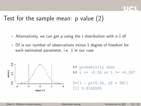
• Alternatively, we can get p using the t distribution with n-1 df
• Df is our number of observations minus 1 degree of freedom foreach estimated parameter, i.e. 1 in our case
## probability that
## t <= -0.24 or t >= +0.24?
2*(1 - pt(0.24, df = 99))
[1] 0.8108265
Week 5: Midterm revision session Hypothesis testing Introduction to QM 18 / 35

Test for the sample mean: p value (2)
• Alternatively, we can get p using the t distribution with n-1 df
• Df is our number of observations minus 1 degree of freedom foreach estimated parameter, i.e. 1 in our case
## probability that
## t <= -0.24 or t >= +0.24?
2*(1 - pt(0.24, df = 99))
[1] 0.8108265
Week 5: Midterm revision session Hypothesis testing Introduction to QM 18 / 35
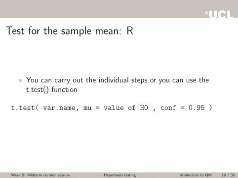
Test for the sample mean: R
• You can carry out the individual steps or you can use thet.test() function
t.test( var.name, mu = value of H0 , conf = 0.95 )
Week 5: Midterm revision session Hypothesis testing Introduction to QM 19 / 35

t-tests for the difference in two means
• Often we are interested in whether the mean for one group isdifferent from the mean for another group
◦ Is woman’s income different to men’s income?◦ Do Democratic and Republican senators receive different
amounts of campaign donations?
• t-tests can also be used to compare the means of two groups
• Requires an interval-level dependent variable (Y) and binaryindependent variable (X)
Week 5: Midterm revision session Hypothesis testing Introduction to QM 20 / 35

t-tests for the difference in two means• What is the null hypothesis?
◦ There is no difference between the means of the two groups inthe population
• The test statistic for the difference in means (for a nullhypothesis of no difference) is
t =YX=0 − YX=1
SE (YX=0 − YX=1)=
YX=0 − YX=1√s2YX=0
nX=0+
s2YX=1
nX=1
• Where s2YX=0and s2YX=1
are the sample variances for each group
◦ The variance (s2Y ) is just the standard deviation (sY ) squared
• nX=0 and nX=1 are the number of observations for each group
Week 5: Midterm revision session Hypothesis testing Introduction to QM 21 / 35

t-tests for the difference in two means• What is the null hypothesis?
◦ There is no difference between the means of the two groups inthe population
• The test statistic for the difference in means (for a nullhypothesis of no difference) is
t =YX=0 − YX=1
SE (YX=0 − YX=1)
=YX=0 − YX=1√
s2YX=0
nX=0+
s2YX=1
nX=1
• Where s2YX=0and s2YX=1
are the sample variances for each group
◦ The variance (s2Y ) is just the standard deviation (sY ) squared
• nX=0 and nX=1 are the number of observations for each group
Week 5: Midterm revision session Hypothesis testing Introduction to QM 21 / 35

t-tests for the difference in two means• What is the null hypothesis?
◦ There is no difference between the means of the two groups inthe population
• The test statistic for the difference in means (for a nullhypothesis of no difference) is
t =YX=0 − YX=1
SE (YX=0 − YX=1)=
YX=0 − YX=1√s2YX=0
nX=0+
s2YX=1
nX=1
• Where s2YX=0and s2YX=1
are the sample variances for each group
◦ The variance (s2Y ) is just the standard deviation (sY ) squared
• nX=0 and nX=1 are the number of observations for each group
Week 5: Midterm revision session Hypothesis testing Introduction to QM 21 / 35

t-tests for the difference in two means• What is the null hypothesis?
◦ There is no difference between the means of the two groups inthe population
• The test statistic for the difference in means (for a nullhypothesis of no difference) is
t =YX=0 − YX=1
SE (YX=0 − YX=1)=
YX=0 − YX=1√s2YX=0
nX=0+
s2YX=1
nX=1
• Where s2YX=0and s2YX=1
are the sample variances for each group
◦ The variance (s2Y ) is just the standard deviation (sY ) squared
• nX=0 and nX=1 are the number of observations for each group
Week 5: Midterm revision session Hypothesis testing Introduction to QM 21 / 35

Test for the difference in means: critical value of t
• Assuming that sample size is large (> 30), the critical t valueis 1.96
• To know the exact critical value, we need to know the degreesof freedom (df)
• You could do it in R using the t.test() function whichcomputes the correct number of df for you
Week 5: Midterm revision session Hypothesis testing Introduction to QM 22 / 35

Test for the difference in means: p value
• Once we know the correct t value, getting the p value is thesame as in the t-test for the sample mean if the sample is large
• If the sample is small, use R’s t.test() function
Week 5: Midterm revision session Hypothesis testing Introduction to QM 23 / 35
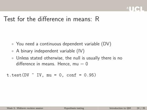
Test for the difference in means: R
• You need a continuous dependent variable (DV)
• A binary independent variable (IV)
• Unless stated otherwise, the null is usually there is nodifference in means. Hence, mu = 0
t.test(DV ~ IV, mu = 0, conf = 0.95)
Week 5: Midterm revision session Hypothesis testing Introduction to QM 24 / 35

Overview
1 Administrative information
2 Answer advice
3 Hypothesis testing
4 Simple linear regression
5 Multiple linear regression
Week 5: Midterm revision session Simple linear regression Introduction to QM 25 / 35

Simple linear regression: intuition
• How are two phenomena (X and Y) related?
Week 5: Midterm revision session Simple linear regression Introduction to QM 26 / 35

Linear relationships• The most straightforward way of describing the relationship
between two variables is with a line• A line can be represented by this expression: Y = α + βX
●
−2 −1 0 1 2
−2
−1
01
2
α = 0.2 and β = 0.7
X−axis
Y−
axis
α = 0.2
β = 0.7
• α is the intercept: the valueof Y where X = 0
• β is the slope: the amountthat Y increases when Xincreases by one unit
• Here, a one-unit increase inX is associated with a0.7-unit increase in Y
Week 5: Midterm revision session Simple linear regression Introduction to QM 27 / 35
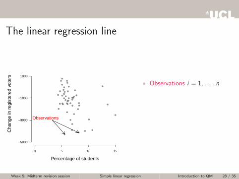
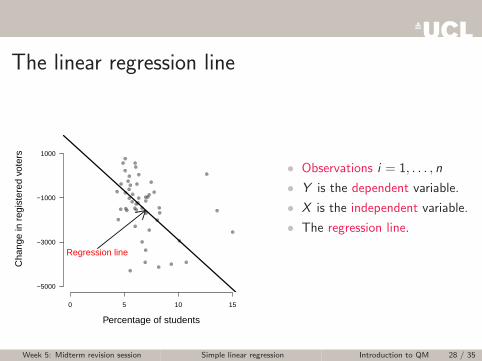
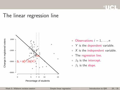
The linear regression line
0 5 10 15
Percentage of students
Observations
−5000
−3000
−1000
1000
Cha
nge
in r
egis
tere
d vo
ters
• Observations i = 1, . . . , n
• Y is the dependent variable.
• X is the independent variable.
• The regression line.
• β0 is the intercept.
• β1 is the slope.
Week 5: Midterm revision session Simple linear regression Introduction to QM 28 / 35

The linear regression line
0 5 10 15
Percentage of students
−5000
−3000
−1000
1000
Cha
nge
in r
egis
tere
d vo
ters
Dependent variable
• Observations i = 1, . . . , n
• Y is the dependent variable.
• X is the independent variable.
• The regression line.
• β0 is the intercept.
• β1 is the slope.
Week 5: Midterm revision session Simple linear regression Introduction to QM 28 / 35

The linear regression line
0 5 10 15
Percentage of students
−5000
−3000
−1000
1000
Cha
nge
in r
egis
tere
d vo
ters
Independent variable
• Observations i = 1, . . . , n
• Y is the dependent variable.
• X is the independent variable.
• The regression line.
• β0 is the intercept.
• β1 is the slope.
Week 5: Midterm revision session Simple linear regression Introduction to QM 28 / 35
The linear regression line
0 5 10 15
Percentage of students
−5000
−3000
−1000
1000
Cha
nge
in r
egis
tere
d vo
ters
Regression line
• Observations i = 1, . . . , n
• Y is the dependent variable.
• X is the independent variable.
• The regression line.
• β0 is the intercept.
• β1 is the slope.
Week 5: Midterm revision session Simple linear regression Introduction to QM 28 / 35

The linear regression line
0 5 10 15
Percentage of students
−5000
−3000
−1000
1000
Cha
nge
in r
egis
tere
d vo
ters β0 • Observations i = 1, . . . , n
• Y is the dependent variable.
• X is the independent variable.
• The regression line.
• β0 is the intercept.
• β1 is the slope.
Week 5: Midterm revision session Simple linear regression Introduction to QM 28 / 35
The linear regression line
0 5 10 15
Percentage of students
−5000
−3000
−1000
1000
Cha
nge
in r
egis
tere
d vo
ters
7 8
β1 = ∆(Y) ∆(X)
• Observations i = 1, . . . , n
• Y is the dependent variable.
• X is the independent variable.
• The regression line.
• β0 is the intercept.
• β1 is the slope.
Week 5: Midterm revision session Simple linear regression Introduction to QM 28 / 35

Application to voter registration
• For the regression of registration on the percentage ofstudents we obtain:
DV: ∆voters βk , (σβk)
(Intercept) 1532.69(192.41)
students −444.97(26.99)
R2 0.32N. 573
where the numbers in brackets are the standard errors of thecoefficients.
Week 5: Midterm revision session Simple linear regression Introduction to QM 29 / 35

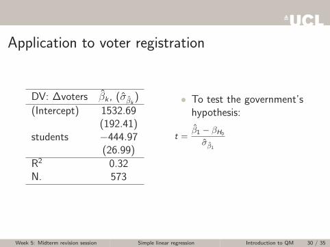
Application to voter registration
DV: ∆voters βk , (σβk)
(Intercept) 1532.69(192.41)
students −444.97(26.99)
R2 0.32N. 573
• To test the government’shypothesis:
t =β1 − βH0
σβ1
=−445− 0
27≈ −16.48
• Can we reject the nullhypothesis at α = 0.05?
Week 5: Midterm revision session Simple linear regression Introduction to QM 30 / 35

Application to voter registration
DV: ∆voters βk , (σβk)
(Intercept) 1532.69(192.41)
students −444.97(26.99)
R2 0.32N. 573
• To test the government’shypothesis:
t =β1 − βH0
σβ1
=−445− 0
27
≈ −16.48
• Can we reject the nullhypothesis at α = 0.05?
Week 5: Midterm revision session Simple linear regression Introduction to QM 30 / 35

Application to voter registration
DV: ∆voters βk , (σβk)
(Intercept) 1532.69(192.41)
students −444.97(26.99)
R2 0.32N. 573
• To test the government’shypothesis:
t =β1 − βH0
σβ1
=−445− 0
27≈ −16.48
• Can we reject the nullhypothesis at α = 0.05?
Week 5: Midterm revision session Simple linear regression Introduction to QM 30 / 35

Application to voter registration
DV: ∆voters βk , (σβk)
(Intercept) 1532.69(192.41)
students −444.97(26.99)
R2 0.32N. 573
• To test the government’shypothesis:
t =β1 − βH0
σβ1
=−445− 0
27≈ −16.48
• Can we reject the nullhypothesis at α = 0.05?
Week 5: Midterm revision session Simple linear regression Introduction to QM 30 / 35

Application to voter registration
t =β1 − βH0
σβ1
=−445− 0
27≈ −16.48
• The probability of observing a value of the t-statistic outsidethe interval [−1.96, 1.96] is less than five percent under thestandard normal distribution.
• As the t-statistic is clearly outside this interval, the probabilitythat H0 is correct is less than five percent.
• We can therefore reject the government’s claim at the fivepercent significance level.
Week 5: Midterm revision session Simple linear regression Introduction to QM 31 / 35
Application to voter registration
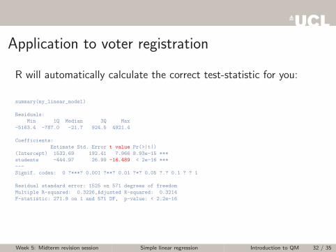
R will automatically calculate the correct test-statistic for you:
summary(my_linear_model)
Residuals:
Min 1Q Median 3Q Max
-5163.4 -787.0 -21.7 924.5 4921.4
Coefficients:
Estimate Std. Error t value Pr(>|t|)
(Intercept) 1532.69 192.41 7.966 8.93e-15 ***
students -444.97 26.99 -16.489 < 2e-16 ***
---
Signif. codes: 0 ?***? 0.001 ?**? 0.01 ?*? 0.05 ?.? 0.1 ? ? 1
Residual standard error: 1525 on 571 degrees of freedom
Multiple R-squared: 0.3226,Adjusted R-squared: 0.3214
F-statistic: 271.9 on 1 and 571 DF, p-value: < 2.2e-16
Week 5: Midterm revision session Simple linear regression Introduction to QM 32 / 35

Overview
1 Administrative information
2 Answer advice
3 Hypothesis testing
4 Simple linear regression
5 Multiple linear regression
Week 5: Midterm revision session Multiple linear regression Introduction to QM 33 / 35

Multiple linear regression: intuition
• We can control for confounders with multiple linear regression
Week 5: Midterm revision session Multiple linear regression Introduction to QM 34 / 35

More than two independent variables
## Specify the model with 3 independent variables
linear_model_3 <- lm(AfD ~ christian + east
+ migrantfraction , data = results)
## Output in a nice format
screenreg(list(linear_model_1, linear_model_2, linear_model_3))
===================================================
Model 1 Model 2 Model 3
---------------------------------------------------
(Intercept) 21.29 *** 7.82 *** 11.78 ***
(0.76) (1.30) (1.90)
christian -0.16 *** 0.03 0.00
(0.01) (0.02) (0.02)
eastTRUE 11.77 *** 9.14 ***
(0.99) (1.35)
migrantfraction -0.09 **
(0.03)
---------------------------------------------------
R^2 0.36 0.56 0.58
Adj. R^2 0.35 0.56 0.57
Num. obs. 299 299 299
===================================================
*** p < 0.001, ** p < 0.01, * p < 0.05
• The coefficient onmigrantfraction
(β3) is negative andsignificant
• The coefficient oneast (β2) is smallerin model 3
• The R2 has increased
Week 5: Midterm revision session Multiple linear regression Introduction to QM 35 / 35


