Week 6: Linear Regression with Two Regressors Brandon Stewart 1 Princeton October 17, 19, 2016 1 These slides are heavily influenced by Matt Blackwell, Adam Glynn and Jens Hainmueller. Stewart (Princeton) Week 6: Two Regressors October 17, 19, 2016 1 / 132
Transcript
Week 6: Linear Regression with Two Regressors
Brandon Stewart1
Princeton
October 17, 19, 2016
1These slides are heavily influenced by Matt Blackwell, Adam Glynn and JensHainmueller.
Stewart (Princeton) Week 6: Two Regressors October 17, 19, 2016 1 / 132
Where We’ve Been and Where We’re Going...
Last WeekI mechanics of OLS with one variableI properties of OLS
This WeekI Monday:
F adding a second variableF new mechanics
I Wednesday:F omitted variable biasF multicollinearityF interactions
Next WeekI multiple regression
Long RunI probability → inference → regression
Questions?
Stewart (Princeton) Week 6: Two Regressors October 17, 19, 2016 2 / 132
1 Two Examples
2 Adding a Binary Variable
3 Adding a Continuous Covariate
4 Once More With Feeling
5 OLS Mechanics and Partialing Out
6 Fun With Red and Blue
7 Omitted Variables
8 Multicollinearity
9 Dummy Variables
10 Interaction Terms
11 Polynomials
12 Conclusion
13 Fun With Interactions
Stewart (Princeton) Week 6: Two Regressors October 17, 19, 2016 3 / 132
Why Do We Want More Than One Predictor?
Summarize more information for descriptive inference
Improve the fit and predictive power of our model
Control for confounding factors for causal inference
Model non-linearities (e.g. Y = β0 + β1X + β2X2)
Model interactive effects (e.g. Y = β0 + β1X + β2X2 + β3X1X2)
Stewart (Princeton) Week 6: Two Regressors October 17, 19, 2016 4 / 132
Example 1: Cigarette Smokers and Pipe Smokers
Stewart (Princeton) Week 6: Two Regressors October 17, 19, 2016 5 / 132
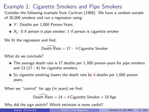
Example 1: Cigarette Smokers and Pipe SmokersConsider the following example from Cochran (1968). We have a random sampleof 20,000 smokers and run a regression using:
Y : Deaths per 1,000 Person-Years.
X1: 0 if person is pipe smoker; 1 if person is cigarette smoker
We fit the regression and find:
Death Rate = 17− 4 Cigarette Smoker
What do we conclude?
The average death rate is 17 deaths per 1, 000 person-years for pipe smokersand 13 (17 - 4) for cigarette smokers.
So cigarette smoking lowers the death rate by 4 deaths per 1,000 personyears.
When we “control” for age (in years) we find:
Death Rate = 14 + 4 Cigarette Smoker + 10 Age
Why did the sign switch? Which estimate is more useful?Stewart (Princeton) Week 6: Two Regressors October 17, 19, 2016 6 / 132
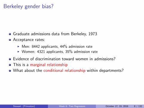
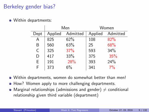
Example 2: Berkeley Graduate Admissions
Stewart (Princeton) Week 6: Two Regressors October 17, 19, 2016 7 / 132
Within departments, women do somewhat better than men!
How? Women apply to more challenging departments.
Marginal relationships (admissions and gender) 6= conditionalrelationship given third variable (department)
Stewart (Princeton) Week 6: Two Regressors October 17, 19, 2016 9 / 132
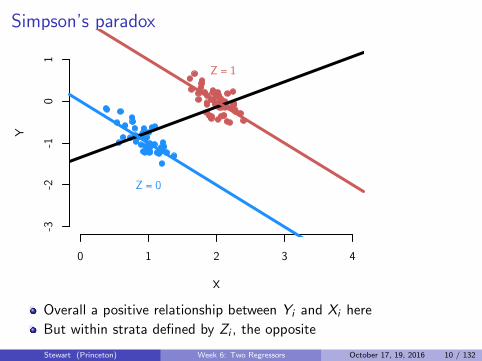
Simpson’s paradox
0 1 2 3 4
-3-2
-10
1
X
Y
Z = 0
Z = 1
Overall a positive relationship between Yi and Xi here
But within strata defined by Zi , the opposite
Stewart (Princeton) Week 6: Two Regressors October 17, 19, 2016 10 / 132
Simpson’s paradox
Simpson’s paradox arises in many contexts- particularly where there isselection on ability
It is a particular problem in medical or demographic contexts, e.g.kidney stones, low-birth weight paradox.
Cochran’s 1968 study is also a case of Simpson’s paradox, he originallysought to compare cigarette to cigar smoking, he found that cigarsmokers had higher mortality rates than cigarette smokers, but at anyage level, cigarette smokers had higher mortality than cigar smokers.
Instance of a more general problem called the ecological inference fallacy
Stewart (Princeton) Week 6: Two Regressors October 17, 19, 2016 11 / 132
Basic idea
Old goal: estimate the mean of Y as a function of some independentvariable, X :
E[Yi |Xi ]
For continuous X ’s, we modeled the CEF/regression function with aline:
Yi = β0 + β1Xi + ui
New goal: estimate the relationship of two variables, Yi and Xi ,conditional on a third variable, Zi :
Yi = β0 + β1Xi + β2Zi + ui
β’s are the population parameters we want to estimate
Stewart (Princeton) Week 6: Two Regressors October 17, 19, 2016 12 / 132
Why control for another variable
Descriptive
I get a sense for the relationships in the data.I describe more precisely our quantity of interest
Predictive
I We can usually make better predictions about the dependent variablewith more information on independent variables.
Causal
I Block potential confounding, which is when X doesn’t cause Y , butonly appears to because a third variable Z causally affects both ofthem.
I Xi : ice cream sales on day iI Yi : drowning deaths on day iI Zi : ??
Stewart (Princeton) Week 6: Two Regressors October 17, 19, 2016 13 / 132
1 Two Examples
2 Adding a Binary Variable
3 Adding a Continuous Covariate
4 Once More With Feeling
5 OLS Mechanics and Partialing Out
6 Fun With Red and Blue
7 Omitted Variables
8 Multicollinearity
9 Dummy Variables
10 Interaction Terms
11 Polynomials
12 Conclusion
13 Fun With Interactions
Stewart (Princeton) Week 6: Two Regressors October 17, 19, 2016 14 / 132
Regression with Two Explanatory VariablesExample: data from Fish (2002) “Islam and Authoritarianism.” WorldPolitics. 55: 4-37. Data from 157 countries.
Variables of interest:I Y : Level of democracy, measured as the 10-year average of Freedom
House ratings
I X1: Country income, measured as log(GDP per capita in $1000s)
I X2: Ethnic heterogeneity (continuous) or British colonial heritage(binary)
With one predictor we ask: Does income (X1) predict or explain thelevel of democracy (Y )?
With two predictors we ask questions like: Does income (X1) predictor explain the level of democracy (Y ), once we “control” for ethnicheterogeneity or British colonial heritage (X2)?
The rest of this lecture is designed to explain what is meant by“controlling for another variable” with linear regression.
Stewart (Princeton) Week 6: Two Regressors October 17, 19, 2016 15 / 132
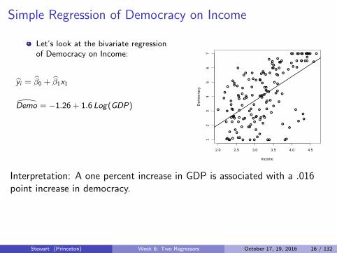
Simple Regression of Democracy on Income
Let’s look at the bivariate regressionof Democracy on Income:
yi = β0 + β1x1
Demo = −1.26 + 1.6 Log(GDP)
Additive Linear RegressionLinear Regression with Interaction terms
Regression with one continuous and one dummy variableAdditive regression with two continuous variablesInference for Slopes
Simple Regression of Democracy on Income
We have looked at theregression of Democracy onIncome several times in thecourse:
yi = β0 + xi β1●
●
●
●
●
●
●●
●
●
●
●
●
●
●
●
●
●
●
●
●
●
●
●
●
●
●
●
●
●
●
●
●
●
●
●
●
●
●
●
●
●
●
●
●
●
●
●
●
●
●
●
●
●
●
●
●
●
●
●
●
●
●
●
●
●
●
●
●
●
●
●
●
●
●
●
●
●
●
●
●
●
●
●
●●
●
●
●
●
●
●
●
●
●
●
●
●
●
●
●
●
●
●
●●
●
●
●
●
●
●
●
●
●
●
●
●
●
●
●
●
●
●
●
●
●
●
●
●
●
●
● ●
●
●
●
●
●
●
●
●
●
●
●
●
●
●
●
●
●
●
●
●
●
●
2.0 2.5 3.0 3.5 4.0 4.5
12
34
56
7
Income
Dem
ocra
cyGov2000: Quantitative Methodology for Political Science I
Interpretation: A one percent increase in GDP is associated with a .016point increase in democracy.
Stewart (Princeton) Week 6: Two Regressors October 17, 19, 2016 16 / 132
Simple Regression of Democracy on Income
But we can use more information inour prediction equation.
For example, some countries were
originally British colonies and others
were not:
I Former British colonies tend tohave higher levels of democracy
I Non-colony countries tend to
have lower levels of democracy
Additive Linear RegressionLinear Regression with Interaction terms
Regression with one continuous and one dummy variableAdditive regression with two continuous variablesInference for Slopes
Adding covariates
We may want to use moreinformation in our predictionequation.For example, some countrieswere originally British coloniesand others were not.
Former British coloniestend to be higherOther countries tend to belower
●
●
●
●
●
●
●●
●
●
●
●
●
●
●
●
●
●
●
●
●
●
●
●
●
●
●
●
●
●
●
●
●
●
●
●
●
●
●
●
●
●
●
●
●
●
●
●
●
●
●
●
●
●
●
●
●
●
●
●
●
●
●
●
●
●
●
●
●
●
●
●
●
●
●
●
●
●
●
●
●
●
●
●
●●
●
●
●
●
●
●
●
●
●
●
●
●
●
●
●
●
●
●
●●
●
●
●
●
●
●
●
●
●
●
●
●
●
●
●
●
●
●
●
●
●
●
●
●
●
●
● ●
●
●
●
●
●
●
●
●
●
●
●
●
●
●
●
●
●
●
●
●
●
●
2.0 2.5 3.0 3.5 4.0 4.5
12
34
56
7
Income
Dem
ocra
cy
●
●
●
●●
●
●
●
●
●
●
●
●
●
●
●
●
●
●
●
●
●
●
●
●
●
●
●
●
●
●
●
●
●
●
●
●
●
●
●
●
●
●
●
●
●
●
●
●
●
●
●
●
●
●
●
●
●
●
●
●
●
●
●
●
●
●
●
●
●
●
●
●
●
●
●●
●
●
●
●
●●
●
●
●
●
●
●
●
●●
●
● ●
●
●
●
●
●
●
●
●
●
●
●
●
●
●
●
●
●
●
●
●
●
●
●
●
●
●
●
●
●
●
●
●
●
●
●
●
●
●
●
●
●
●
●
● ●
●
●
●
● ●
●
●
●
●
●
●
●
●
●
●
●
Gov2000: Quantitative Methodology for Political Science I
Stewart (Princeton) Week 6: Two Regressors October 17, 19, 2016 17 / 132
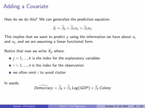
Adding a Covariate
How do we do this? We can generalize the prediction equation:
yi = β0 + β1x1i + β2x2i
This implies that we want to predict y using the information we have about x1and x2, and we are assuming a linear functional form.
Notice that now we write Xji where:
j = 1, ..., k is the index for the explanatory variables
i = 1, ..., n is the index for the observation
we often omit i to avoid clutter
In words:Democracy = β0 + β1 Log(GDP) + β2 Colony
Stewart (Princeton) Week 6: Two Regressors October 17, 19, 2016 18 / 132
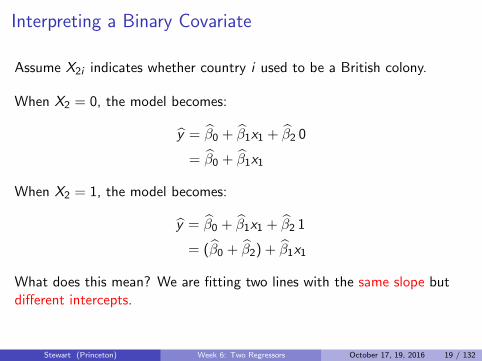
Interpreting a Binary Covariate
Assume X2i indicates whether country i used to be a British colony.
When X2 = 0, the model becomes:
y = β0 + β1x1 + β2 0
= β0 + β1x1
When X2 = 1, the model becomes:
y = β0 + β1x1 + β2 1
= (β0 + β2) + β1x1
What does this mean? We are fitting two lines with the same slope butdifferent intercepts.
Stewart (Princeton) Week 6: Two Regressors October 17, 19, 2016 19 / 132
Regression of Democracy on IncomeFrom R, we obtain estimatesβ0, β1, β2:
Coefficients:
Estimate
(Intercept) -1.5060
GDP90LGN 1.7059
BRITCOL 0.5881
Non-British colonies:
y = β0 + β1x1
y = −1.5 + 1.7 x1
Former British colonies:
y = (β0 + β2) + β1x1
y = −.92 + 1.7 x1
Additive Linear RegressionLinear Regression with Interaction terms
Regression with one continuous and one dummy variableAdditive regression with two continuous variablesInference for Slopes
What does this mean?
Using R, we obtain estimatesfor β0, β1, and β2
lm(Democracy ~ Income + BritishColony)
Coefficients:(Intercept) Income BritishColony
-1.527 1.711 0.592
Non-British colonies:
yi = −1.527 + 1.711xi
British colonies:
yi = −0.935 + 1.711xi2.0 2.5 3.0 3.5 4.0 4.5
12
34
56
7
IncomeD
emoc
racy
●
●
●
●●
●
●
●
●
●
●
●
●
●
●
●
●
●
●
●
●
●
●
●
●
●
●
●
●
●
●
●
●
●
●
●
●
●
●
●
●
●
●
●
●
●
●
●
●
●
●
●
●
●
●
●
●
●
●
●
●
●
●
●
●
●
●
●
●
●
●
●
●
●
●
●●
●
●
●
●
●●
●
●
●
●
●
●
●
●●
●
● ●
●
●
●
●
●
●
●
●
●
●
●
●
●
●
●
●
●
●
●
●
●
●
●
●
●
●
●
●
●
●
●
●
●
●
●
●
●
●
●
●
●
●
●
● ●
●
●
●
● ●
●
●
●
●
●
●
●
●
●
●
●
Gov2000: Quantitative Methodology for Political Science I
Stewart (Princeton) Week 6: Two Regressors October 17, 19, 2016 20 / 132
β0 = −1.5 is the intercept for theprediction line for non-British colonies.
β1 = 1.7 is the slope for both lines.
β2 = .58 is the vertical distancebetween the two lines for Ex-Britishcolonies and non-colonies respectively
Additive Linear RegressionLinear Regression with Interaction terms
Regression with one continuous and one dummy variableAdditive regression with two continuous variablesInference for Slopes
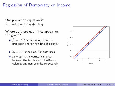
What does this mean?Our prediction equation is
yi = −1.527+1.711xi +0.592zi
Where do these quantitiesappear on the graph?
β0 = −1.527 is theintercept for the predictionline for non-Britishcolonies.β1 = 1.711 is the slope forboth lines.β2 = 0.592 is the verticaldistance between the twolines.
0 1 2 3 4 5
−2
02
46
Income
Dem
ocra
cy
ββ2
Gov2000: Quantitative Methodology for Political Science I
Stewart (Princeton) Week 6: Two Regressors October 17, 19, 2016 21 / 132
1 Two Examples
2 Adding a Binary Variable
3 Adding a Continuous Covariate
4 Once More With Feeling
5 OLS Mechanics and Partialing Out
6 Fun With Red and Blue
7 Omitted Variables
8 Multicollinearity
9 Dummy Variables
10 Interaction Terms
11 Polynomials
12 Conclusion
13 Fun With Interactions
Stewart (Princeton) Week 6: Two Regressors October 17, 19, 2016 22 / 132
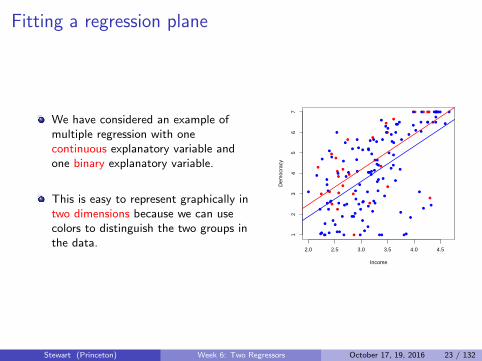
Fitting a regression plane
We have considered an example ofmultiple regression with onecontinuous explanatory variable andone binary explanatory variable.
This is easy to represent graphically intwo dimensions because we can usecolors to distinguish the two groups inthe data.
Additive Linear RegressionLinear Regression with Interaction terms
Regression with one continuous and one dummy variableAdditive regression with two continuous variablesInference for Slopes
Fitting a regression plane
We have considered anexample of multiple regressionwith one continuousexplanatory variable and onebinary explanatory variable.
This is easy to representgraphically in two dimensionsbecause we can use colors todistinguish the two groups inthe data.
2.0 2.5 3.0 3.5 4.0 4.5
12
34
56
7
Income
Dem
ocra
cy
●
●
●
●●
●
●
●
●
●
●
●
●
●
●
●
●
●
●
●
●
●
●
●
●
●
●
●
●
●
●
●
●
●
●
●
●
●
●
●
●
●
●
●
●
●
●
●
●
●
●
●
●
●
●
●
●
●
●
●
●
●
●
●
●
●
●
●
●
●
●
●
●
●
●
●●
●
●
●
●
●●
●
●
●
●
●
●
●
●●
●
● ●
●
●
●
●
●
●
●
●
●
●
●
●
●
●
●
●
●
●
●
●
●
●
●
●
●
●
●
●
●
●
●
●
●
●
●
●
●
●
●
●
●
●
●
● ●
●
●
●
● ●
●
●
●
●
●
●
●
●
●
●
●
Gov2000: Quantitative Methodology for Political Science I
Stewart (Princeton) Week 6: Two Regressors October 17, 19, 2016 23 / 132
Regression of Democracy on Income
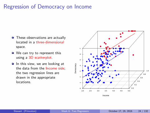
These observations are actuallylocated in a three-dimensionalspace.
We can try to represent thisusing a 3D scatterplot.
In this view, we are looking atthe data from the Income side;the two regression lines aredrawn in the appropriatelocations.
2.0 2.5 3.0 3.5 4.0 4.5 5.0
01
23
45
67
0.0
0.2
0.4
0.6
0.8
1.0
Income
Col
ony
Dem
ocra
cy
●
●
●●●●
●
●
●
●
●
●
●
●
●
●
●
●
●
●
●
●
●
●
●
●
●
●
●
●
●
●
●
●●●●●●●
●
●
●
●●
●
●
●
●
●
●
●
●
●
●
●●
●
●
●
●●●
●
●
●
●
●
●
●
●
●
●●
●
●
●
●
●
●
●
●
●
●
●
●●
●
●
●
●
●
●
●
●
●●
●
●
●●
●
●
●
●
●
●●
●
●
●
●
●
●
●
●
●
●
●
●
●●
●
●
●
●
●
●
●
●
●
●
●
●
●
●
●
●●
●
●
●
●
●
●
●
●●
●
●
●
●●
●
●
●
●
●
●
●
●
●
●
●
●
●
●
●
●
●
●
●
●
●
●
●
●
●
●
●
●
● ● ●●
●
●
Stewart (Princeton) Week 6: Two Regressors October 17, 19, 2016 24 / 132
Regression of Democracy on Income
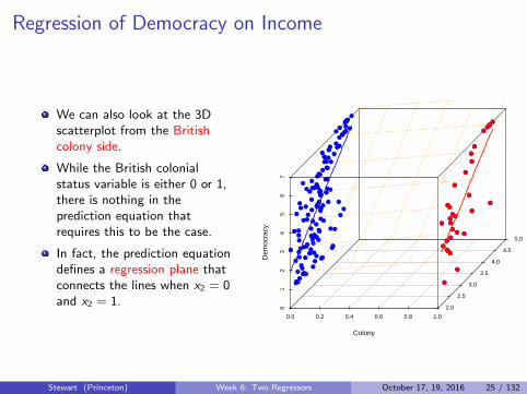
We can also look at the 3Dscatterplot from the Britishcolony side.
While the British colonialstatus variable is either 0 or 1,there is nothing in theprediction equation thatrequires this to be the case.
In fact, the prediction equationdefines a regression plane thatconnects the lines when x2 = 0and x2 = 1.
0.0 0.2 0.4 0.6 0.8 1.0
01
23
45
67
2.0
2.5
3.0
3.5
4.0
4.5
5.0
Colony
Inco
me
Dem
ocra
cy
●
●
●●●●●●●
●●
●
●
●
●
●●
●
●
●●
●
●
●
●
●●
●
●
●
●●
●
●
●
●●●
●
●
●
●
●
●
●
●
●
●
●
●
●●
●●
●
●
●
●
●
●
●
●
●
●
●
●●
●
●
●
●
●
● ●
●
●
●●
●
●
●
●●
●
●
●
●
●
●●
●
●
●
●
●
●
●
●
●
●
●
●
●
●
●
●
●
●
●●
●
●
●
●
●
●
●
●
●
●
●
●
●
●●
●
●
●
●
●
●●
●
●●
● ●
●
●
●
●
●
●
●●
●
●
●
●
●
●
●
●
●
●
●
●
●
●
●
●
●
●
●
●
●
●
●
●
●
●
●
●
●
●
●
●
●
●
●
●
●●●●
●
●
Stewart (Princeton) Week 6: Two Regressors October 17, 19, 2016 25 / 132
Regression with two continuous variables
Since we fit a regression plane to the data whenever we have twoexplanatory variables, it is easy to move to a case with twocontinuous explanatory variables.
For example, we might want to use:
I X1 Income and X2 Ethnic HeterogeneityI Y Democracy
Stewart (Princeton) Week 6: Two Regressors October 17, 19, 2016 26 / 132
Regression of Democracy on Income
We can plot the points in a 3Dscatterplot.
R returns:
I β0 = −.71I β1 = 1.6 for IncomeI β2 = −.6 for Ethnic
Heterogeneity
How does this lookgraphically?
These estimates define aregression plane through thedata.
Additive Linear RegressionLinear Regression with Interaction terms
Regression with one continuous and one dummy variableAdditive regression with two continuous variablesInference for Slopes
Fitting a regression plane
We can plot the points in a 3Dscatterplot.
R returns the followingestimates:
β0 = −0.717β1 = 1.573β2 = −0.550
These estimates define aregression plane through thedata.
2.0 2.5 3.0 3.5 4.0 4.5 5.0
12
34
56
7
0.00.2
0.40.6
0.81.0
Income
Eth
nicH
eter
ogen
eity
Dem
ocra
cy
●
●
●
●
●
●
●
●
●
●
●
●
●
●
●●
●
● ●
●
●
●
●
●
●
●
●
●
●
●
●
●
●
●
●
●
●
●
●
●
●
●
●
●
●
●
●
●
●
●
●
●
●
●
●
●
●
●
●
●
●
●
●
●
●
●
●●
●
●
●
●
●
●
●
●
●
●
●
●
●●
●
●
●
●
●
●
●
●
●
●
●
●
●
●
●
●
●
●
●
●
●● ●
●
●
●
●
●●
●
●
●
●
●
●●
●
●
●
●
●
●
●
●
●
●
●
●
● ●
●
●●
●
●●
●
●
●
●
●
●
●
●
●
●
Gov2000: Quantitative Methodology for Political Science IStewart (Princeton) Week 6: Two Regressors October 17, 19, 2016 27 / 132
Interpreting a Continuous Covariate
The coefficient estimates have a similar interpretation in this case asthey did in the Income-British Colony example.
For example, β1 = 1.6 represents our prediction of the difference inDemocracy between two observations that differ by one unit ofIncome but have the same value of Ethnic Heterogeneity.
The slope estimates have partial effect or ceteris paribusinterpretations:
∂(y = β0 + β1X1 + β2X2)
∂X1= β1
Stewart (Princeton) Week 6: Two Regressors October 17, 19, 2016 28 / 132
Interpreting a Continuous Covariate
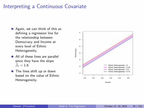
Again, we can think of this asdefining a regression line forthe relationship betweenDemocracy and Income atevery level of EthnicHeterogeneity.
All of these lines are parallelsince they have the slopeβ1 = 1.6
The lines shift up or downbased on the value of EthnicHeterogeneity.
Additive Linear RegressionLinear Regression with Interaction terms
Regression with one continuous and one dummy variableAdditive regression with two continuous variablesInference for Slopes
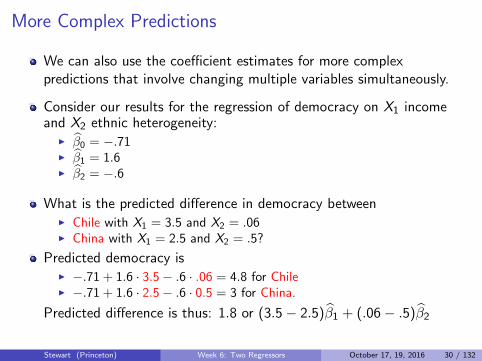
What does this mean?
Again, we can think of this asdefining a regression line forthe relationship betweenDemocracy and Income atevery level of EthnicHeterogeneity.
All of these lines are parallelsince they have the slope β1.
The lines shift up or downbased on the value of EthnicHeterogeneity.
Predicted difference is thus: 1.8 or (3.5− 2.5)β1 + (.06− .5)β2
Stewart (Princeton) Week 6: Two Regressors October 17, 19, 2016 30 / 132
1 Two Examples
2 Adding a Binary Variable
3 Adding a Continuous Covariate
4 Once More With Feeling
5 OLS Mechanics and Partialing Out
6 Fun With Red and Blue
7 Omitted Variables
8 Multicollinearity
9 Dummy Variables
10 Interaction Terms
11 Polynomials
12 Conclusion
13 Fun With Interactions
Stewart (Princeton) Week 6: Two Regressors October 17, 19, 2016 31 / 132
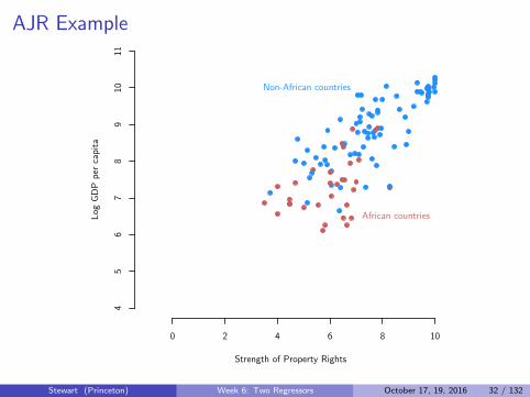
AJR Example
0 2 4 6 8 10
45
67
89
1011
Strength of Property Rights
Log
GDP
per c
apita
African countries
Non-African countries
Stewart (Princeton) Week 6: Two Regressors October 17, 19, 2016 32 / 132
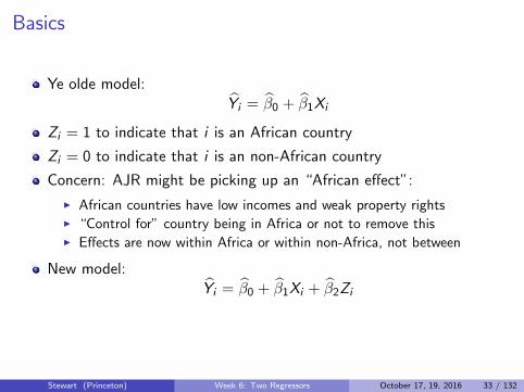
Basics
Ye olde model:Yi = β0 + β1Xi
Zi = 1 to indicate that i is an African country
Zi = 0 to indicate that i is an non-African country
Concern: AJR might be picking up an “African effect”:
I African countries have low incomes and weak property rightsI “Control for” country being in Africa or not to remove thisI Effects are now within Africa or within non-Africa, not between
New model:Yi = β0 + β1Xi + β2Zi
Stewart (Princeton) Week 6: Two Regressors October 17, 19, 2016 33 / 132
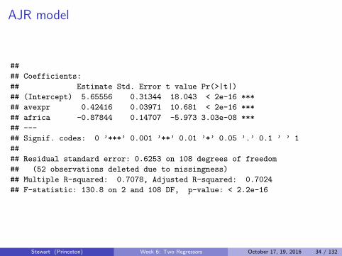
## F-statistic: 130.8 on 2 and 108 DF, p-value: < 2.2e-16
Stewart (Princeton) Week 6: Two Regressors October 17, 19, 2016 34 / 132
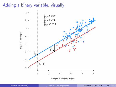
Two lines in one regression
How can we interpret this model?
Plug in two possible values for Zi and rearrange
When Zi = 0:Yi = β0 + β1Xi + β2Zi
= β0 + β1Xi + β2 × 0
= β0 + β1Xi
When Zi = 1:Yi = β0 + β1Xi + β2Zi
= β0 + β1Xi + β2 × 1
= (β0 + β2) + β1Xi
Two different intercepts, same slope
Stewart (Princeton) Week 6: Two Regressors October 17, 19, 2016 35 / 132
Example interpretation of the coefficients
Let’s review what we’ve seen so far:
Intercept for Xi Slope for Xi
Non-African country (Zi = 0) β0 β1African country (Zi = 1) β0 + β2 β1
In this example, we have:
Yi = 5.656 + 0.424× Xi − 0.878× Zi
We can read these as:
I β0: average log income for non-African country (Zi = 0) with propertyrights measured at 0 is 5.656
I β1: A one-unit increase in property rights is associated with a 0.424increase in average log incomes for two African countries (or for twonon-African countries)
I β2: there is a -0.878 average difference in log income per capitabetween African and non-African counties conditional on propertyrights
Stewart (Princeton) Week 6: Two Regressors October 17, 19, 2016 36 / 132
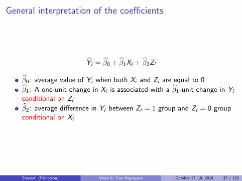
General interpretation of the coefficients
Yi = β0 + β1Xi + β2Zi
β0: average value of Yi when both Xi and Zi are equal to 0
β1: A one-unit change in Xi is associated with a β1-unit change in Yi
conditional on Zi
β2: average difference in Yi between Zi = 1 group and Zi = 0 groupconditional on Xi
Stewart (Princeton) Week 6: Two Regressors October 17, 19, 2016 37 / 132
Adding a binary variable, visually
0 2 4 6 8 10
45
67
89
1011
Strength of Property Rights
Log
GDP
per c
apita
β0
β0 + β2
β2
β0 = 5.656β1 = 0.424β2 = -0.878
Stewart (Princeton) Week 6: Two Regressors October 17, 19, 2016 38 / 132
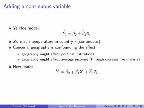
Adding a continuous variable
Ye olde model:Yi = β0 + β1Xi
Zi : mean temperature in country i (continuous)
Concern: geography is confounding the effect
I geography might affect political institutionsI geography might affect average incomes (through diseases like malaria)
New model:Yi = β0 + β1Xi + β2Zi
Stewart (Princeton) Week 6: Two Regressors October 17, 19, 2016 39 / 132
## F-statistic: 18.45 on 1 and 58 DF, p-value: 6.733e-05
Stewart (Princeton) Week 6: Two Regressors October 17, 19, 2016 47 / 132
Regression of log income on the residuals
## (Intercept) avexpr.res
## 8.0542783 0.4056757
## (Intercept) avexpr meantemp
## 6.80627375 0.40567575 -0.06024937
Stewart (Princeton) Week 6: Two Regressors October 17, 19, 2016 48 / 132
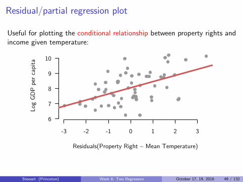
Residual/partial regression plot
Useful for plotting the conditional relationship between property rights andincome given temperature:
-3 -2 -1 0 1 2 3
6
7
8
9
10
Residuals(Property Right ~ Mean Temperature)
Log
GDP
per c
apita
Stewart (Princeton) Week 6: Two Regressors October 17, 19, 2016 49 / 132
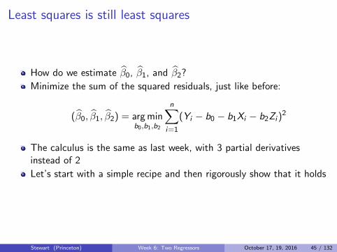
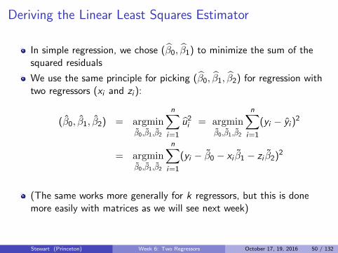
Deriving the Linear Least Squares Estimator
In simple regression, we chose (β0, β1) to minimize the sum of thesquared residuals
We use the same principle for picking (β0, β1, β2) for regression withtwo regressors (xi and zi ):
(β0, β1, β2) = argminβ0,β1,β2
n∑i=1
u2i = argminβ0,β1,β2
n∑i=1
(yi − yi )2
= argminβ0,β1,β2
n∑i=1
(yi − β0 − xi β1 − zi β2)2
(The same works more generally for k regressors, but this is donemore easily with matrices as we will see next week)
Stewart (Princeton) Week 6: Two Regressors October 17, 19, 2016 50 / 132
Deriving the Linear Least Squares Estimator
We want to minimize the following quantitity with respect to (β0, β1, β2):
S(β0, β1, β2) =n∑
i=1
(yi − β0 − β1xi − β2zi )2
Plan is conceptually the same as before
1 Take the partial derivatives of S with respect to β0, β1 and β2.
2 Set each of the partial derivatives to 0 to obtain the first orderconditions.
3 Substitute β0, β1, β2 for β0, β1, β2 and solve for β0, β1, β2 to obtainthe OLS estimator.
Stewart (Princeton) Week 6: Two Regressors October 17, 19, 2016 51 / 132
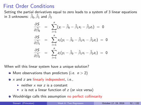
First Order ConditionsSetting the partial derivatives equal to zero leads to a system of 3 linear equationsin 3 unknowns: β0, β1 and β2
∂S
∂β0=
n∑i=1
(yi − β0 − β1xi − β2zi ) = 0
∂S
∂β1=
n∑i=1
xi (yi − β0 − β1xi − β2zi ) = 0
∂S
∂β2=
n∑i=1
zi (yi − β0 − β1xi − β2zi ) = 0
When will this linear system have a unique solution?
More observations than predictors (i.e. n > 2)
x and z are linearly independent, i.e.,
I neither x nor z is a constantI x is not a linear function of z (or vice versa)
Wooldridge calls this assumption no perfect collinearity
Stewart (Princeton) Week 6: Two Regressors October 17, 19, 2016 52 / 132
The OLS Estimator
The OLS estimator for (β0, β1, β2) can be written as
β0 = y − β1x − β2z
β1 =Cov(x , y)Var(z)− Cov(z , y)Cov(x , z)
Var(x)Var(z)− Cov(x , z)2
β2 =Cov(z , y)Var(x)− Cov(x , y)Cov(z , x)
Var(x)Var(z)− Cov(x , z)2
For (β0, β1, β2) to be well-defined we need:
Var(x)Var(z) 6= Cov(x , z)2
Condition fails if:
1 If x or z is a constant (⇒ Var(x)Var(z) = Cov(x , z) = 0)
2 One explanatory variable is an exact linear function of another(⇒ Cor(x , z) = 1 ⇒ Var(x)Var(z) = Cov(x , z)2)
Stewart (Princeton) Week 6: Two Regressors October 17, 19, 2016 53 / 132
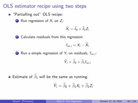
“Partialling Out” Interpretation of the OLS Estimator
Assume Y = β0 + β1X + β2Z + u. Another way to write the OLS estimator is:
β1 =
∑ni rxz,i yi∑ni r
2xz,i
where rxz,i are the residuals from the regression of X on Z :
X = λ+ δZ + rxz
In other words, both of these regressions yield identical estimates β1:
y = γ0 + β1rxz and y = β0 + β1x + β2z
δ is correlation between X and Z . What is our estimator β1 if δ = 0?
rxz = x − λ = xi − x so β1 =
∑ni rxz,i yi∑ni r
2xz,i
=
∑ni (xi − x) yi∑ni (xi − x)2
That is, same as the simple regresson of Y on X alone.
Stewart (Princeton) Week 6: Two Regressors October 17, 19, 2016 54 / 132
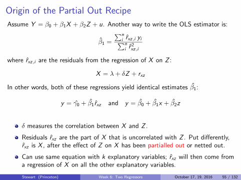
Origin of the Partial Out Recipe
Assume Y = β0 + β1X + β2Z + u. Another way to write the OLS estimator is:
β1 =
∑ni rxz,i yi∑ni r
2xz,i
where rxz,i are the residuals from the regression of X on Z :
X = λ+ δZ + rxz
In other words, both of these regressions yield identical estimates β1:
y = γ0 + β1rxz and y = β0 + β1x + β2z
δ measures the correlation between X and Z .
Residuals rxz are the part of X that is uncorrelated with Z . Put differently,rxz is X , after the effect of Z on X has been partialled out or netted out.
Can use same equation with k explanatory variables; rxz will then come froma regression of X on all the other explanatory variables.
Stewart (Princeton) Week 6: Two Regressors October 17, 19, 2016 55 / 132
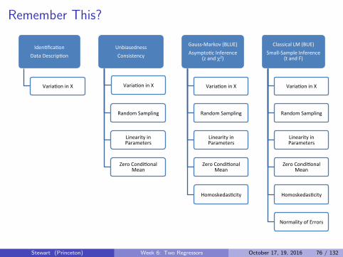
OLS assumptions for unbiasedness
When we have more than one independent variable, we need thefollowing assumptions in order for OLS to be unbiased:
1 LinearityYi = β0 + β1Xi + β2Zi + ui
2 Random/iid sample3 No perfect collinearity4 Zero conditional mean error
E[ui |Xi ,Zi ] = 0
Stewart (Princeton) Week 6: Two Regressors October 17, 19, 2016 56 / 132
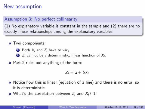
New assumption
Assumption 3: No perfect collinearity
(1) No explanatory variable is constant in the sample and (2) there are noexactly linear relationships among the explanatory variables.
Two components
1 Both Xi and Zi have to vary.2 Zi cannot be a deterministic, linear function of Xi .
Part 2 rules out anything of the form:
Zi = a + bXi
Notice how this is linear (equation of a line) and there is no error, soit is deterministic.
What’s the correlation between Zi and Xi? 1!
Stewart (Princeton) Week 6: Two Regressors October 17, 19, 2016 57 / 132
Perfect collinearity example (I)
Simple example:
I Xi = 1 if a country is not in Africa and 0 otherwise.I Zi = 1 if a country is in Africa and 0 otherwise.
But, clearly we have the following:
Zi = 1− Xi
These two variables are perfectly collinear.
What about the following:
I Xi = incomeI Zi = X 2
i
Do we have to worry about collinearity here?
No! Because while Zi is a deterministic function of Xi , it is not alinear function of Xi .
Stewart (Princeton) Week 6: Two Regressors October 17, 19, 2016 58 / 132
R and perfect collinearity
R, and all other packages, will drop one of the variables if there isperfect collinearity:
##
## Coefficients: (1 not defined because of singularities)
## F-statistic: 69.68 on 1 and 146 DF, p-value: 4.87e-14
Stewart (Princeton) Week 6: Two Regressors October 17, 19, 2016 59 / 132
Perfect collinearity example (II)
Another example:
I Xi = mean temperature in CelsiusI Zi = 1.8Xi + 32 (mean temperature in Fahrenheit)
## (Intercept) meantemp meantemp.f
## 10.8454999 -0.1206948 NA
Stewart (Princeton) Week 6: Two Regressors October 17, 19, 2016 60 / 132
OLS assumptions for large-sample inference
For large-sample inference and calculating SEs, we need the two-variableversion of the Gauss-Markov assumptions:
1 LinearityYi = β0 + β1Xi + β2Zi + ui
2 Random/iid sample
3 No perfect collinearity
4 Zero conditional mean error
E[ui |Xi ,Zi ] = 0
5 Homoskedasticityvar[ui |Xi ,Zi ] = σ2u
Stewart (Princeton) Week 6: Two Regressors October 17, 19, 2016 61 / 132
Inference with two independent variables in large samples
We have our OLS estimate β1We have an estimate of the standard error for that coefficient, SE [β1].
Under assumption 1-5, in large samples, we’ll have the following:
β1 − β1SE [β1]
∼ N(0, 1)
The same holds for the other coefficient:
β2 − β2SE [β2]
∼ N(0, 1)
Inference is exactly the same in large samples!
Hypothesis tests and CIs are good to go
The SE’s will change, though
Stewart (Princeton) Week 6: Two Regressors October 17, 19, 2016 62 / 132
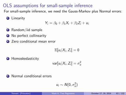
OLS assumptions for small-sample inferenceFor small-sample inference, we need the Gauss-Markov plus Normal errors:
1 LinearityYi = β0 + β1Xi + β2Zi + ui
2 Random/iid sample
3 No perfect collinearity
4 Zero conditional mean error
E[ui |Xi ,Zi ] = 0
5 Homoskedasticityvar[ui |Xi ,Zi ] = σ2u
6 Normal conditional errors
ui ∼ N(0, σ2u)
Stewart (Princeton) Week 6: Two Regressors October 17, 19, 2016 63 / 132
Inference with two independent variables in small samples
Under assumptions 1-6, we have the following small change to oursmall-n sampling distribution:
β1 − β1SE [β1]
∼ tn−3
The same is true for the other coefficient:
β2 − β2SE [β2]
∼ tn−3
Why n − 3?
I We’ve estimated another parameter, so we need to take off anotherdegree of freedom.
small adjustments to the critical values and the t-values for ourhypothesis tests and confidence intervals.
Stewart (Princeton) Week 6: Two Regressors October 17, 19, 2016 64 / 132
1 Two Examples
2 Adding a Binary Variable
3 Adding a Continuous Covariate
4 Once More With Feeling
5 OLS Mechanics and Partialing Out
6 Fun With Red and Blue
7 Omitted Variables
8 Multicollinearity
9 Dummy Variables
10 Interaction Terms
11 Polynomials
12 Conclusion
13 Fun With Interactions
Stewart (Princeton) Week 6: Two Regressors October 17, 19, 2016 65 / 132
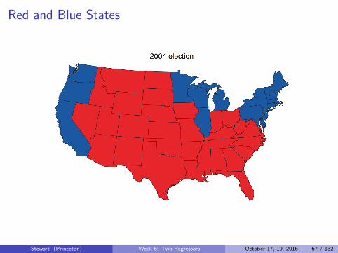
Red State Blue State
Stewart (Princeton) Week 6: Two Regressors October 17, 19, 2016 66 / 132
Red and Blue States
Stewart (Princeton) Week 6: Two Regressors October 17, 19, 2016 67 / 132
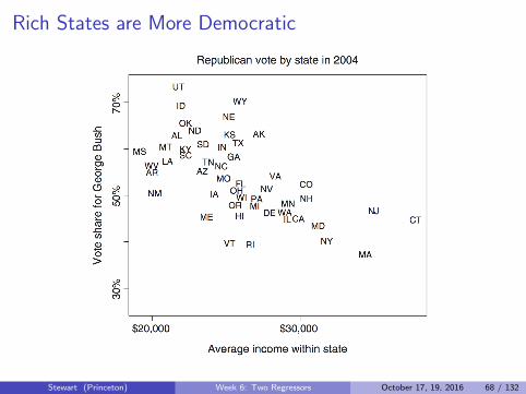
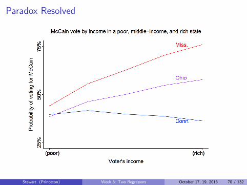
Rich States are More Democratic
Stewart (Princeton) Week 6: Two Regressors October 17, 19, 2016 68 / 132
But Rich People are More Republican
Stewart (Princeton) Week 6: Two Regressors October 17, 19, 2016 69 / 132
Paradox Resolved
Stewart (Princeton) Week 6: Two Regressors October 17, 19, 2016 70 / 132
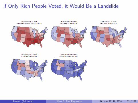
If Only Rich People Voted, it Would Be a Landslide
Stewart (Princeton) Week 6: Two Regressors October 17, 19, 2016 71 / 132
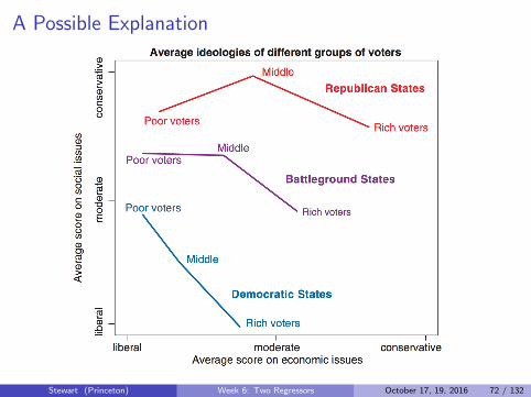
A Possible Explanation
Stewart (Princeton) Week 6: Two Regressors October 17, 19, 2016 72 / 132
References
Acemoglu, Daron, Simon Johnson, and James A. Robinson. “The colonialorigins of comparative development: An empirical investigation.”American Economic Review. 91(5). 2001: 1369-1401.
Fish, M. Steven. ”Islam and authoritarianism.” World politics 55(01).2002: 4-37.
Gelman, Andrew. Red state, blue state, rich state, poor state: whyAmericans vote the way they do. Princeton University Press, 2009.
Stewart (Princeton) Week 6: Two Regressors October 17, 19, 2016 73 / 132
Where We’ve Been and Where We’re Going...
Last WeekI mechanics of OLS with one variableI properties of OLS
This WeekI Monday:
F adding a second variableF new mechanics
I Wednesday:F omitted variable biasF multicollinearityF interactions
Next WeekI multiple regression
Long RunI probability → inference → regression
Questions?
Stewart (Princeton) Week 6: Two Regressors October 17, 19, 2016 74 / 132
1 Two Examples
2 Adding a Binary Variable
3 Adding a Continuous Covariate
4 Once More With Feeling
5 OLS Mechanics and Partialing Out
6 Fun With Red and Blue
7 Omitted Variables
8 Multicollinearity
9 Dummy Variables
10 Interaction Terms
11 Polynomials
12 Conclusion
13 Fun With Interactions
Stewart (Princeton) Week 6: Two Regressors October 17, 19, 2016 75 / 132
Stewart (Princeton) Week 6: Two Regressors October 17, 19, 2016 76 / 132
Unbiasedness revisited
True model:Yi = β0 + β1Xi + β2Zi + ui
Assumptions 1-4 ⇒ we get unbiased estimates of the coefficients
What happens if we ignore the Zi and just run the simple linearregression with just Xi?
Misspecified model:
Yi = β0 + β1Xi + u∗i u∗i = β2Zi + ui
OLS estimates from the misspecified model:
Yi = β0 + β1Xi
Stewart (Princeton) Week 6: Two Regressors October 17, 19, 2016 77 / 132
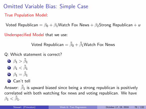
Omitted Variable Bias: Simple Case
True Population Model:
Voted Republican = β0 + β1Watch Fox News + β2Strong Republican + u
Underspecified Model that we use:
Voted Republican = β0 + β1Watch Fox News
Q: Which statement is correct?
1 β1 > β12 β1 < β13 β1 = β14 Can’t tell
Answer: β1 is upward biased since being a strong republican is positivelycorrelated with both watching fox news and voting republican. We haveβ1 < β1.
Stewart (Princeton) Week 6: Two Regressors October 17, 19, 2016 78 / 132
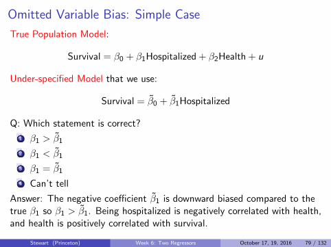
Omitted Variable Bias: Simple Case
True Population Model:
Survival = β0 + β1Hospitalized + β2Health + u
Under-specified Model that we use:
Survival = β0 + β1Hospitalized
Q: Which statement is correct?
1 β1 > β12 β1 < β13 β1 = β14 Can’t tell
Answer: The negative coefficient β1 is downward biased compared to thetrue β1 so β1 > β1. Being hospitalized is negatively correlated with health,and health is positively correlated with survival.
Stewart (Princeton) Week 6: Two Regressors October 17, 19, 2016 79 / 132
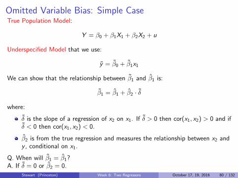
Omitted Variable Bias: Simple CaseTrue Population Model:
Y = β0 + β1X1 + β2X2 + u
Underspecified Model that we use:
y = β0 + β1x1
We can show that the relationship between β1 and β1 is:
β1 = β1 + β2 · δ
where:
δ is the slope of a regression of x2 on x1. If δ > 0 then cor(x1, x2) > 0 and ifδ < 0 then cor(x1, x2) < 0.
β2 is from the true regression and measures the relationship between x2 andy , conditional on x1.
Q. When will β1 = β1?A. If δ = 0 or β2 = 0.
Stewart (Princeton) Week 6: Two Regressors October 17, 19, 2016 80 / 132
Omitted Variable Bias: Simple Case
We take expectations to see what the bias will be:
β1 = β1 + β2 · δE [β1 | X ] = E [β1 + β2 · δ | X ]
= E [β1 | X ] + E [β2 | X ] · δ (δ nonrandom given x)
= β1 + β2 · δ (given assumptions 1-4)
So
Bias[β1 | X ] = E [β1 | X ]− β1 = β2 · δ
So the bias depends on the relationship between x2 and x1, our δ, and therelationship between x2 and y , our β2.
Any variable that is correlated with an included X and the outcome Y iscalled a confounder.
Stewart (Princeton) Week 6: Two Regressors October 17, 19, 2016 81 / 132
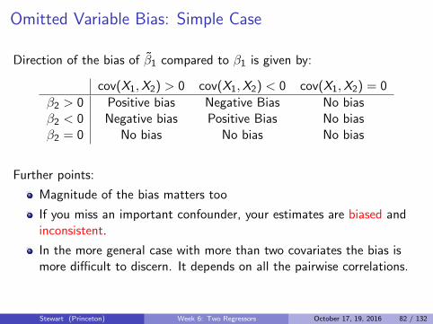
Omitted Variable Bias: Simple Case
Direction of the bias of β1 compared to β1 is given by:
cov(X1,X2) > 0 cov(X1,X2) < 0 cov(X1,X2) = 0
β2 > 0 Positive bias Negative Bias No biasβ2 < 0 Negative bias Positive Bias No biasβ2 = 0 No bias No bias No bias
Further points:
Magnitude of the bias matters too
If you miss an important confounder, your estimates are biased andinconsistent.
In the more general case with more than two covariates the bias ismore difficult to discern. It depends on all the pairwise correlations.
Stewart (Princeton) Week 6: Two Regressors October 17, 19, 2016 82 / 132
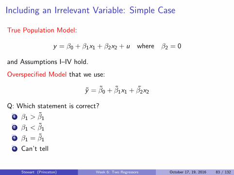
Including an Irrelevant Variable: Simple Case
True Population Model:
y = β0 + β1x1 + β2x2 + u where β2 = 0
and Assumptions I–IV hold.
Overspecified Model that we use:
y = β0 + β1x1 + β2x2
Q: Which statement is correct?
1 β1 > β12 β1 < β13 β1 = β14 Can’t tell
Stewart (Princeton) Week 6: Two Regressors October 17, 19, 2016 83 / 132
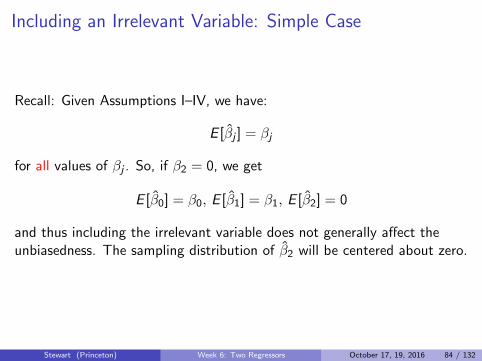
Including an Irrelevant Variable: Simple Case
Recall: Given Assumptions I–IV, we have:
E [βj ] = βj
for all values of βj . So, if β2 = 0, we get
E [β0] = β0, E [β1] = β1, E [β2] = 0
and thus including the irrelevant variable does not generally affect theunbiasedness. The sampling distribution of β2 will be centered about zero.
Stewart (Princeton) Week 6: Two Regressors October 17, 19, 2016 84 / 132
1 Two Examples
2 Adding a Binary Variable
3 Adding a Continuous Covariate
4 Once More With Feeling
5 OLS Mechanics and Partialing Out
6 Fun With Red and Blue
7 Omitted Variables
8 Multicollinearity
9 Dummy Variables
10 Interaction Terms
11 Polynomials
12 Conclusion
13 Fun With Interactions
Stewart (Princeton) Week 6: Two Regressors October 17, 19, 2016 85 / 132
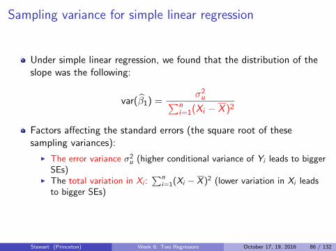
Sampling variance for simple linear regression
Under simple linear regression, we found that the distribution of theslope was the following:
var(β1) =σ2u∑n
i=1(Xi − X )2
Factors affecting the standard errors (the square root of thesesampling variances):
I The error variance σ2u (higher conditional variance of Yi leads to bigger
SEs)I The total variation in Xi :
∑ni=1(Xi − X )2 (lower variation in Xi leads
to bigger SEs)
Stewart (Princeton) Week 6: Two Regressors October 17, 19, 2016 86 / 132
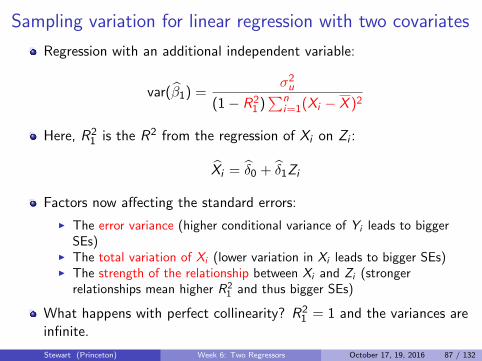
Sampling variation for linear regression with two covariates
Regression with an additional independent variable:
var(β1) =σ2u
(1− R21 )∑n
i=1(Xi − X )2
Here, R21 is the R2 from the regression of Xi on Zi :
Xi = δ0 + δ1Zi
Factors now affecting the standard errors:
I The error variance (higher conditional variance of Yi leads to biggerSEs)
I The total variation of Xi (lower variation in Xi leads to bigger SEs)I The strength of the relationship between Xi and Zi (stronger
relationships mean higher R21 and thus bigger SEs)
What happens with perfect collinearity? R21 = 1 and the variances are
infinite.
Stewart (Princeton) Week 6: Two Regressors October 17, 19, 2016 87 / 132
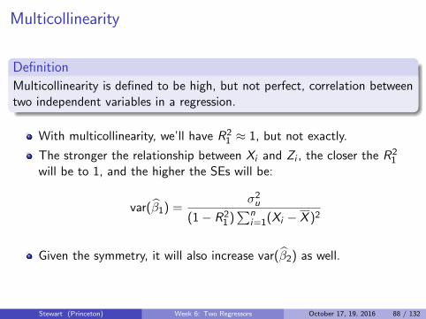
Multicollinearity
Definition
Multicollinearity is defined to be high, but not perfect, correlation betweentwo independent variables in a regression.
With multicollinearity, we’ll have R21 ≈ 1, but not exactly.
The stronger the relationship between Xi and Zi , the closer the R21
will be to 1, and the higher the SEs will be:
var(β1) =σ2u
(1− R21 )∑n
i=1(Xi − X )2
Given the symmetry, it will also increase var(β2) as well.
Stewart (Princeton) Week 6: Two Regressors October 17, 19, 2016 88 / 132
Intuition for multicollinearity
Remember the OLS recipe:
I β1 from regression of Yi on rxz,iI rxz,i are the residuals from the regression of Xi on Zi
Estimated coefficient:
β1 =
∑ni=1 rxz,iYi∑ni=1 r
2xz,i
When Zi and Xi have a strong relationship, then the residuals willhave low variation
We explain away a lot of the variation in Xi through Zi .
Low variation in an independent variable (here, rxz,i ) high SEs
Basically, there is less residual variation left in Xi after “partiallingout” the effect of Zi
Stewart (Princeton) Week 6: Two Regressors October 17, 19, 2016 89 / 132
Effects of multicollinearity
No effect on the bias of OLS.
Only increases the standard errors.
Really just a sample size problem:
I If Xi and Zi are extremely highly correlated, you’re going to need amuch bigger sample to accurately differentiate between their effects.
Stewart (Princeton) Week 6: Two Regressors October 17, 19, 2016 90 / 132
How Do We Detect Multicollinearity?
The best practice is to directly compute Cor(X1,X2) before running yourregression.
But you might (and probably will) forget to do so. Even then, you candetect multicollinearity from your regression result:
I Large changes in the estimated regression coefficients when a predictorvariable is added or deleted
I Lack of statistical significance despite high R2
I Estimated regression coefficients have an opposite sign from predicted
A more formal indicator is the variance inflation factor (VIF):
VIF (βj) =1
1− R2j
which measures how much V [βj | X ] is inflated compared to a(hypothetical) uncorrelated data. (where R2
j is the coefficient ofdetermination from the partialing out equation)In R, vif() in the car package.
Stewart (Princeton) Week 6: Two Regressors October 17, 19, 2016 91 / 132
So How Should I Think about Multicollinearity?
Multicollinearity does NOT lead to bias; estimates will be unbiasedand consistent.
Multicollinearity should in fact be seen as a problem ofmicronumerosity, or “too little data.” You can’t ask the OLSestimator to distinguish the partial effects of X1 and X2 if they areessentially the same.
If X1 and X2 are almost the same, why would you want a unique β1and a unique β2? Think about how you would interpret that?
Relax, you got way more important things to worry about!
If possible, get more data
Drop one of the variables, or combine them
Or maybe linear regression is not the right tool
Stewart (Princeton) Week 6: Two Regressors October 17, 19, 2016 92 / 132
1 Two Examples
2 Adding a Binary Variable
3 Adding a Continuous Covariate
4 Once More With Feeling
5 OLS Mechanics and Partialing Out
6 Fun With Red and Blue
7 Omitted Variables
8 Multicollinearity
9 Dummy Variables
10 Interaction Terms
11 Polynomials
12 Conclusion
13 Fun With Interactions
Stewart (Princeton) Week 6: Two Regressors October 17, 19, 2016 93 / 132
Why Dummy Variables?
A dummy variable (a.k.a. indicator variable, binary variable, etc.) is avariable that is coded 1 or 0 only.
We use dummy variables in regression to represent qualitative informationthrough categorical variables such as different subgroups of the sample (e.g.regions, old and young respondents, etc.)
By including dummy variables into our regression function, we can easilyobtain the conditional mean of the outcome variable for each category.
I E.g. does average income vary by region? Are Republicans smarterthan Democrats?
Dummy variables are also used to examine conditional hypothesis viainteraction terms
I E.g. does the effect of education differ by gender?
Stewart (Princeton) Week 6: Two Regressors October 17, 19, 2016 94 / 132
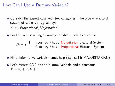
How Can I Use a Dummy Variable?
Consider the easiest case with two categories. The type of electoralsystem of country i is given by:
Xi ∈ {Proportional ,Majoritarian}
For this we use a single dummy variable which is coded like:
Di =
{1 if country i has a Majoritarian Electoral System0 if country i has a Proportional Electoral System
Hint: Informative variable names help (e.g. call it MAJORITARIAN)
Let’s regress GDP on this dummy variable and a constant:Y = β0 + β1D + u
Stewart (Princeton) Week 6: Two Regressors October 17, 19, 2016 95 / 132
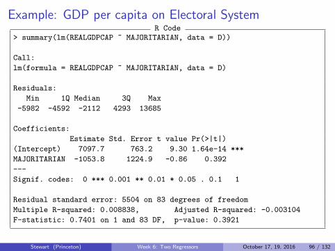
Example: GDP per capita on Electoral SystemR Code
> summary(lm(REALGDPCAP ~ MAJORITARIAN, data = D))
Call:
lm(formula = REALGDPCAP ~ MAJORITARIAN, data = D)
Residuals:
Min 1Q Median 3Q Max
-5982 -4592 -2112 4293 13685
Coefficients:
Estimate Std. Error t value Pr(>|t|)
(Intercept) 7097.7 763.2 9.30 1.64e-14 ***
MAJORITARIAN -1053.8 1224.9 -0.86 0.392
---
Signif. codes: 0 *** 0.001 ** 0.01 * 0.05 . 0.1 1
Residual standard error: 5504 on 83 degrees of freedom
F-statistic: 0.7401 on 1 and 83 DF, p-value: 0.3921
Stewart (Princeton) Week 6: Two Regressors October 17, 19, 2016 96 / 132
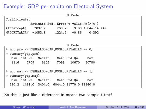
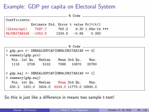
Example: GDP per capita on Electoral System
R CodeCoefficients:
Estimate Std. Error t value Pr(>|t|)
(Intercept) 7097.7 763.2 9.30 1.64e-14 ***
MAJORITARIAN -1053.8 1224.9 -0.86 0.392
R Code> gdp.pro <- D$REALGDPCAP[D$MAJORITARIAN == 0]
> summary(gdp.pro)
Min. 1st Qu. Median Mean 3rd Qu. Max.
1116 2709 5102 7098 10670 20780
> gdp.maj <- D$REALGDPCAP[D$MAJORITARIAN == 1]
> summary(gdp.maj)
Min. 1st Qu. Median Mean 3rd Qu. Max.
530.2 1431.0 3404.0 6044.0 11770.0 18840.0
So this is just like a difference in means two sample t-test!
Stewart (Princeton) Week 6: Two Regressors October 17, 19, 2016 97 / 132
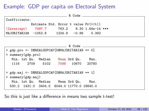
Example: GDP per capita on Electoral System
R CodeCoefficients:
Estimate Std. Error t value Pr(>|t|)
(Intercept) 7097.7 763.2 9.30 1.64e-14 ***
MAJORITARIAN -1053.8 1224.9 -0.86 0.392
R Code> gdp.pro <- D$REALGDPCAP[D$MAJORITARIAN == 0]
> summary(gdp.pro)
Min. 1st Qu. Median Mean 3rd Qu. Max.
1116 2709 5102 7098 10670 20780
> gdp.maj <- D$REALGDPCAP[D$MAJORITARIAN == 1]
> summary(gdp.maj)
Min. 1st Qu. Median Mean 3rd Qu. Max.
530.2 1431.0 3404.0 6044.0 11770.0 18840.0
So this is just like a difference in means two sample t-test!
Stewart (Princeton) Week 6: Two Regressors October 17, 19, 2016 98 / 132
Example: GDP per capita on Electoral System
R CodeCoefficients:
Estimate Std. Error t value Pr(>|t|)
(Intercept) 7097.7 763.2 9.30 1.64e-14 ***
MAJORITARIAN -1053.8 1224.9 -0.86 0.392
R Code> gdp.pro <- D$REALGDPCAP[D$MAJORITARIAN == 0]
> summary(gdp.pro)
Min. 1st Qu. Median Mean 3rd Qu. Max.
1116 2709 5102 7098 10670 20780
> gdp.maj <- D$REALGDPCAP[D$MAJORITARIAN == 1]
> summary(gdp.maj)
Min. 1st Qu. Median Mean 3rd Qu. Max.
530.2 1431.0 3404.0 6044.0 11770.0 18840.0
So this is just like a difference in means two sample t-test!
Stewart (Princeton) Week 6: Two Regressors October 17, 19, 2016 99 / 132
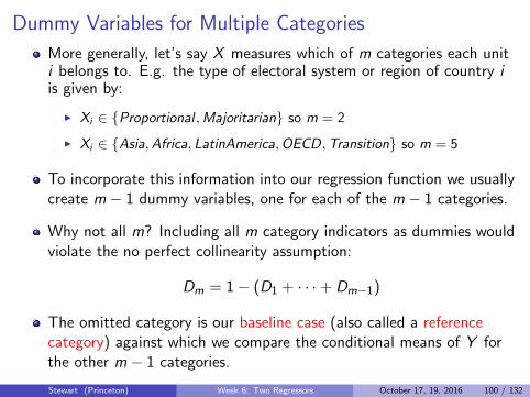
Dummy Variables for Multiple Categories
More generally, let’s say X measures which of m categories each uniti belongs to. E.g. the type of electoral system or region of country iis given by:
I Xi ∈ {Proportional ,Majoritarian} so m = 2
I Xi ∈ {Asia,Africa, LatinAmerica,OECD,Transition} so m = 5
To incorporate this information into our regression function we usuallycreate m − 1 dummy variables, one for each of the m − 1 categories.
Why not all m? Including all m category indicators as dummies wouldviolate the no perfect collinearity assumption:
Dm = 1− (D1 + · · ·+ Dm−1)
The omitted category is our baseline case (also called a referencecategory) against which we compare the conditional means of Y forthe other m − 1 categories.
Stewart (Princeton) Week 6: Two Regressors October 17, 19, 2016 100 / 132
Example: Regions of the World
Consider the case of our “polytomous” variable world region withm = 5:
Xi ∈ {Asia,Africa, LatinAmerica,OECD,Transition}This five-category classification can be represented in the regressionequation by introducing m − 1 = 4 dummy regressors:
Category D1 D2 D3 D4
Asia 1 0 0 0Africa 0 1 0 0
LatinAmerica 0 0 1 0OECD 0 0 0 1
Transition 0 0 0 0
Our regression equation is:
Y = β0 + β1D1 + β2D2 + β3D3 + β4D4 + u
Stewart (Princeton) Week 6: Two Regressors October 17, 19, 2016 101 / 132
1 Two Examples
2 Adding a Binary Variable
3 Adding a Continuous Covariate
4 Once More With Feeling
5 OLS Mechanics and Partialing Out
6 Fun With Red and Blue
7 Omitted Variables
8 Multicollinearity
9 Dummy Variables
10 Interaction Terms
11 Polynomials
12 Conclusion
13 Fun With Interactions
Stewart (Princeton) Week 6: Two Regressors October 17, 19, 2016 102 / 132
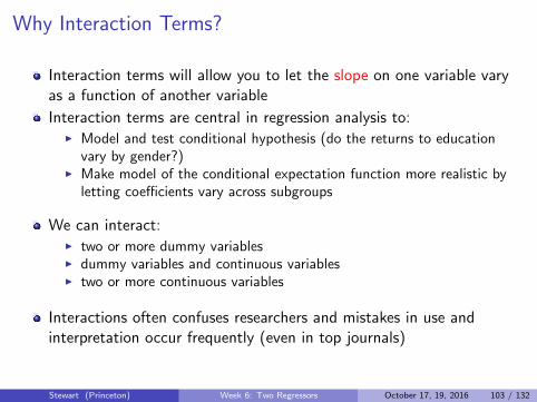
Why Interaction Terms?
Interaction terms will allow you to let the slope on one variable varyas a function of another variable
Interaction terms are central in regression analysis to:I Model and test conditional hypothesis (do the returns to education
vary by gender?)I Make model of the conditional expectation function more realistic by
letting coefficients vary across subgroups
We can interact:I two or more dummy variablesI dummy variables and continuous variablesI two or more continuous variables
Interactions often confuses researchers and mistakes in use andinterpretation occur frequently (even in top journals)
Stewart (Princeton) Week 6: Two Regressors October 17, 19, 2016 103 / 132
Return to the Fish Example
Data comes from Fish (2002), “Islam and Authoritarianism.”
Basic relationship: does more economic development lead to moredemocracy?
We measure economic development with log GDP per capita
We measure democracy with a Freedom House score, 1 (less free) to7 (more free)
Stewart (Princeton) Week 6: Two Regressors October 17, 19, 2016 104 / 132
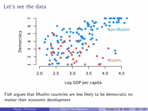
Let’s see the data
2.0 2.5 3.0 3.5 4.0 4.5
12
34
56
7
Log GDP per capita
Dem
ocr
acy
Muslim
Non-Muslim
Fish argues that Muslim countries are less likely to be democratic nomatter their economic development
Stewart (Princeton) Week 6: Two Regressors October 17, 19, 2016 105 / 132
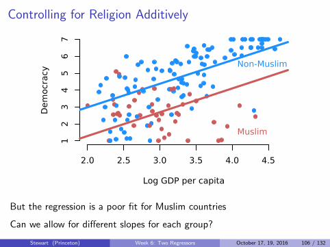
Controlling for Religion Additively
2.0 2.5 3.0 3.5 4.0 4.5
12
34
56
7
Log GDP per capita
Dem
ocr
acy
Muslim
Non-Muslim
But the regression is a poor fit for Muslim countries
Can we allow for different slopes for each group?
Stewart (Princeton) Week 6: Two Regressors October 17, 19, 2016 106 / 132
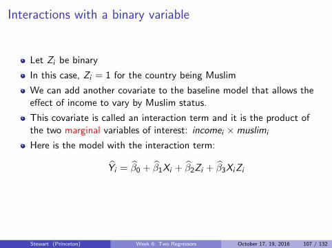
Interactions with a binary variable
Let Zi be binary
In this case, Zi = 1 for the country being Muslim
We can add another covariate to the baseline model that allows theeffect of income to vary by Muslim status.
This covariate is called an interaction term and it is the product ofthe two marginal variables of interest: incomei ×muslimi
Here is the model with the interaction term:
Yi = β0 + β1Xi + β2Zi + β3XiZi
Stewart (Princeton) Week 6: Two Regressors October 17, 19, 2016 107 / 132
Two lines in one regression
Yi = β0 + β1Xi + β2Zi + β3XiZi
How can we interpret this model?
We can plug in the two possible values of Zi
When Zi = 0:Yi = β0 + β1Xi + β2Zi + β3XiZi
= β0 + β1Xi + β2 × 0 + β3Xi × 0
= β0 + β1Xi
When Zi = 1:Yi = β0 + β1Xi + β2Zi + β3XiZi
= β0 + β1Xi + β2 × 1 + β3Xi × 1
= (β0 + β2) + (β1 + β3)Xi
Stewart (Princeton) Week 6: Two Regressors October 17, 19, 2016 108 / 132
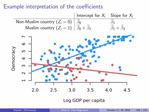
Example interpretation of the coefficients
Intercept for Xi Slope for Xi
Non-Muslim country (Zi = 0) β0 β1Muslim country (Zi = 1) β0 + β2 β1 + β3
2.0 2.5 3.0 3.5 4.0 4.5
12
34
56
7
Log GDP per capita
Dem
ocr
acy
Stewart (Princeton) Week 6: Two Regressors October 17, 19, 2016 109 / 132
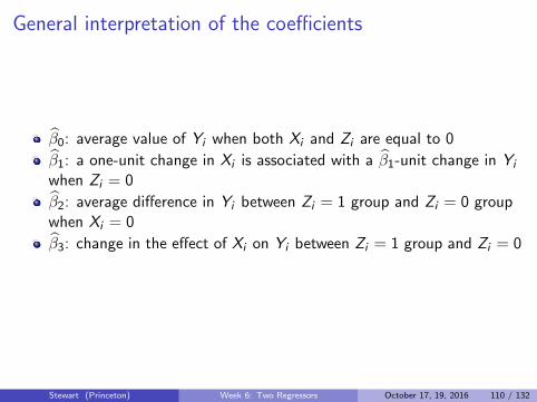
General interpretation of the coefficients
β0: average value of Yi when both Xi and Zi are equal to 0
β1: a one-unit change in Xi is associated with a β1-unit change in Yi
when Zi = 0
β2: average difference in Yi between Zi = 1 group and Zi = 0 groupwhen Xi = 0
β3: change in the effect of Xi on Yi between Zi = 1 group and Zi = 0
Stewart (Princeton) Week 6: Two Regressors October 17, 19, 2016 110 / 132
Lower order terms
Principle of Marginality: Always include the marginal effects(sometimes called the lower order terms)
Imagine we omitted the lower order term for muslim:
0 1 2 3 4
02
46
Log GDP per capita
Dem
ocr
acy
Stewart (Princeton) Week 6: Two Regressors October 17, 19, 2016 111 / 132
Omitting lower order terms
Yi = β0 + β1Xi + 0× Zi + β3XiZi
Intercept for Xi Slope for Xi
Non-Muslim country (Zi = 0) β0 β1Muslim country (Zi = 1) β0 + 0 β1 + β3
Implication: no difference between Muslims and non-Muslims whenincome is 0
Distorts slope estimates.
Very rarely justified.
Yet for some reason people keep doing it.
Stewart (Princeton) Week 6: Two Regressors October 17, 19, 2016 112 / 132
Interactions with two continuous variables
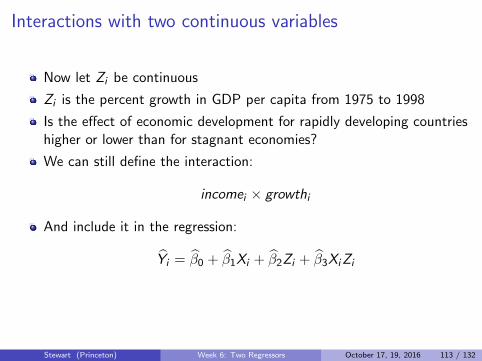
Now let Zi be continuous
Zi is the percent growth in GDP per capita from 1975 to 1998
Is the effect of economic development for rapidly developing countrieshigher or lower than for stagnant economies?
We can still define the interaction:
incomei × growthi
And include it in the regression:
Yi = β0 + β1Xi + β2Zi + β3XiZi
Stewart (Princeton) Week 6: Two Regressors October 17, 19, 2016 113 / 132
Interpretation
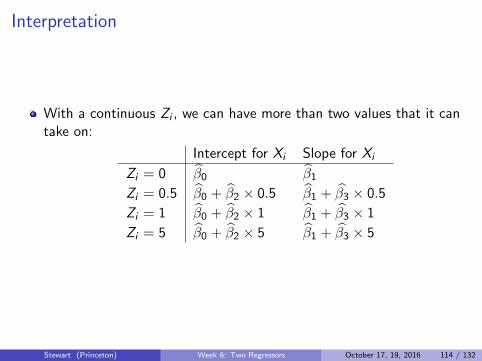
With a continuous Zi , we can have more than two values that it cantake on:
Intercept for Xi Slope for Xi
Zi = 0 β0 β1Zi = 0.5 β0 + β2 × 0.5 β1 + β3 × 0.5
Zi = 1 β0 + β2 × 1 β1 + β3 × 1
Zi = 5 β0 + β2 × 5 β1 + β3 × 5
Stewart (Princeton) Week 6: Two Regressors October 17, 19, 2016 114 / 132
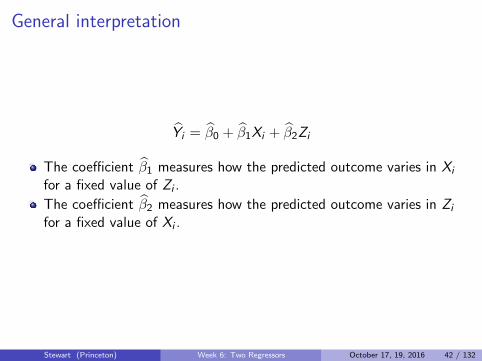
General interpretation
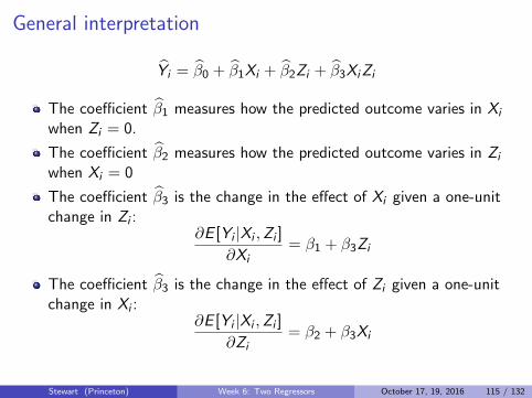
Yi = β0 + β1Xi + β2Zi + β3XiZi
The coefficient β1 measures how the predicted outcome varies in Xi
when Zi = 0.
The coefficient β2 measures how the predicted outcome varies in Zi
when Xi = 0
The coefficient β3 is the change in the effect of Xi given a one-unitchange in Zi :
∂E [Yi |Xi ,Zi ]
∂Xi= β1 + β3Zi
The coefficient β3 is the change in the effect of Zi given a one-unitchange in Xi :
∂E [Yi |Xi ,Zi ]
∂Zi= β2 + β3Xi
Stewart (Princeton) Week 6: Two Regressors October 17, 19, 2016 115 / 132
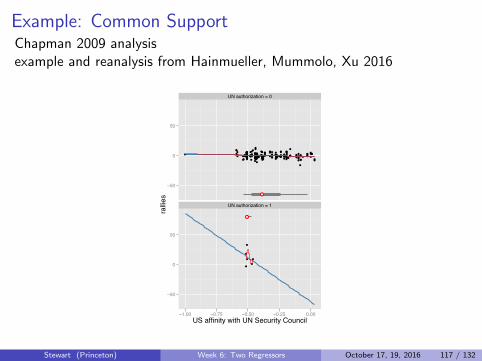
Additional Assumptions
Interaction effects are particularly susceptible to model dependence. Weare making two assumptions for the estimated effects to be meaningful:
1 Linearity of the interaction effect
2 Common support (variation in X throughout the range of Z )
We will talk about checking these assumptions in a few weeks.
Stewart (Princeton) Week 6: Two Regressors October 17, 19, 2016 116 / 132
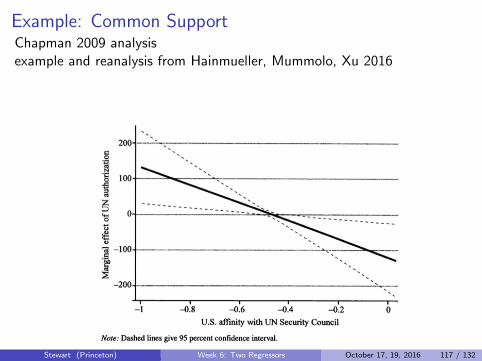
Example: Common SupportChapman 2009 analysisexample and reanalysis from Hainmueller, Mummolo, Xu 2016
Stewart (Princeton) Week 6: Two Regressors October 17, 19, 2016 117 / 132
Example: Common SupportChapman 2009 analysisexample and reanalysis from Hainmueller, Mummolo, Xu 2016
●
●
●●
●●●
●●
●●●●●
●●●●●●●●●
●
●●●●●
●
●
●●
●
●●●●●●●
●●●●
●●
●●●●●
●
●
●
●
●●
●●●●●●
●
●
●●●●●●
●
●●
●●
●●●●
●●●
●
●
●
●●●● ●●●
●●●●●●
●●
●●●
●
●
●
●
●●●●●●●●●
●●●●●●●●●●●●●●●
●●
●●●●●
●
●●●●
●●
●●
●
●●●
●●●
●● ●●
●●●●
●
●
●●
●●●●●●●
●
●● ●●
●
●
●●
●●
●
●
●
●
●
●
●
●
●
●
UN authorization = 0
UN authorization = 1
−50
0
50
−50
0
50
−1.00 −0.75 −0.50 −0.25 0.00US affinity with UN Security Council
rallie
s
Stewart (Princeton) Week 6: Two Regressors October 17, 19, 2016 117 / 132
Summary for Interactions
Do not omit lower order terms (unless you have a strong theory that tellsyou so) because this usually imposes unrealistic restrictions.
Do not interpret the coefficients on the lower terms as marginal effects (theygive the marginal effect only for the case where the other variable is equal tozero)
Produce tables or figures that summarize the conditional marginal effects ofthe variable of interest at plausible different levels of the other variable; usecorrect formula to compute variance for these conditional effects (sum ofcoefficients)
In simple cases the p-value on the interaction term can be used as a testagainst the null of no interaction, but significant tests for the lower orderterms rarely make sense.
Further Reading: Brambor, Clark, and Golder. 2006. Understanding InteractionModels: Improving Empirical Analyses. Political Analysis 14 (1): 63-82.
Hainmueller, Mummolo, Xu. 2016. How Much Should We Trust Estimates fromMultiplicative Interaction Models? Simple Tools to Improve Empirical Practice.Working Paper
Stewart (Princeton) Week 6: Two Regressors October 17, 19, 2016 118 / 132
1 Two Examples
2 Adding a Binary Variable
3 Adding a Continuous Covariate
4 Once More With Feeling
5 OLS Mechanics and Partialing Out
6 Fun With Red and Blue
7 Omitted Variables
8 Multicollinearity
9 Dummy Variables
10 Interaction Terms
11 Polynomials
12 Conclusion
13 Fun With Interactions
Stewart (Princeton) Week 6: Two Regressors October 17, 19, 2016 119 / 132
Polynomial terms
Polynomial terms are a special case of the continuous variableinteractions.
For example, when X1 = X2 in the previous interaction model, we geta quadratic:
Y = β0 + β1X1 + β2X2 + β3X1 X2 + u
Y = β0 + (β1 + β2)X1 + β3X1 X1 + u
Y = β0 + β1X1 + β2X21 + u
This is called a second order polynomial in X1
A third order polynomial is given by:Y = β0 + β1X1 + β2X
21 + β3X
31 + u
Stewart (Princeton) Week 6: Two Regressors October 17, 19, 2016 120 / 132
Polynomial Example: Income and Age
Let’s look at data from theU.S. and examine therelationship between Y: incomeand X: age
We see that a simple linearspecification does not fit thedata very well:Y = β0 + β1X1 + u
A second order polynomial inage fits the data a lot better:Y = β0 + β1X1 + β2X
21 + u
Additive Linear RegressionLinear Regression with Interaction terms
Dummies interacted with continuous variablesInteraction of two continuous variablesHypothesis testing with interaction terms
Quadratic age effect
If we define xi to be age forindividual i and yi to be incomecategory,
Gov2000: Quantitative Methodology for Political Science I
Stewart (Princeton) Week 6: Two Regressors October 17, 19, 2016 122 / 132
Higher Order Polynomials
Approximating data generated with a sine function. Red line is a first degreepolynomial, green line is second degree, orange line is third degree and blue isfourth degree
Stewart (Princeton) Week 6: Two Regressors October 17, 19, 2016 123 / 132
Conclusion
In this brave new world with 2 independent variables:
1 β’s have slightly different interpretations
2 OLS still minimizing the sum of the squared residuals
3 Small adjustments to OLS assumptions and inference
4 Adding or omitting variables in a regression can affect the bias andthe variance of OLS
5 We can optionally consider interactions, but must take care tointerpret them correctly
Stewart (Princeton) Week 6: Two Regressors October 17, 19, 2016 124 / 132
Next Week
OLS in its full glory
Reading:I Practice up on matricesI Fox Chapter 9.1-9.4 (skip 9.1.1-9.1.2) Linear Models in Matrix FormI Aronow and Miller 4.1.2-4.1.4 Regression with Matrix AlgebraI Optional: Fox Chapter 10 Geometry of RegressionI Optional: Imai Chapter 4.3-4.3.3I Optional: Angrist and Pischke Chapter 3.1 Regression Fundamentals
Stewart (Princeton) Week 6: Two Regressors October 17, 19, 2016 125 / 132
1 Two Examples
2 Adding a Binary Variable
3 Adding a Continuous Covariate
4 Once More With Feeling
5 OLS Mechanics and Partialing Out
6 Fun With Red and Blue
7 Omitted Variables
8 Multicollinearity
9 Dummy Variables
10 Interaction Terms
11 Polynomials
12 Conclusion
13 Fun With Interactions
Stewart (Princeton) Week 6: Two Regressors October 17, 19, 2016 126 / 132
Fun With Interactions
Remember that time I mentioned people doing strange things withinteractions?
Brooks and Manza (2006). “Social Policy Responsiveness in DevelopedDemocracies.” American Sociological Review.
Breznau (2015) “The Missing Main Effect of Welfare State Regimes: AReplication of ‘Social Policy Responsiveness in Developed Democracies.”’Sociological Science.
Stewart (Princeton) Week 6: Two Regressors October 17, 19, 2016 127 / 132
Original Argument
Public preferences shape welfare state trajectories over the long term
Democracy empowers the masses, and that empowerment helpsdefine social outcomes
Key model is interaction between liberal/non-liberal and publicpreferences on social spending
but. . . they leave out a main effect.
Stewart (Princeton) Week 6: Two Regressors October 17, 19, 2016 128 / 132
Omitted Term
They omit the marginal term for liberal/non-liberal
This forces the two regression lines to intersect at public preferences= 0.
They mean center so the 0 represents the average over the entiresample
Stewart (Princeton) Week 6: Two Regressors October 17, 19, 2016 129 / 132
What Happens?
Stewart (Princeton) Week 6: Two Regressors October 17, 19, 2016 130 / 132
Moral of the Story
Seriously, don’t omit lower order terms.
<drops mic>
Stewart (Princeton) Week 6: Two Regressors October 17, 19, 2016 131 / 132
References
Acemoglu, Daron, Simon Johnson, and James A. Robinson. “The colonialorigins of comparative development: An empirical investigation.”American Economic Review. 91(5). 2001: 1369-1401.
Fish, M. Steven. ”Islam and authoritarianism.” World politics 55(01).2002: 4-37.
Gelman, Andrew. Red state, blue state, rich state, poor state: whyAmericans vote the way they do. Princeton University Press, 2009.
Stewart (Princeton) Week 6: Two Regressors October 17, 19, 2016 132 / 132