53
8
| Date post: | 29-Feb-2016 |
| Category: |
Documents |
| Upload: | farhan-beigh |
| View: | 4 times |
| Download: | 0 times |

7/18/2019 Week1
http://slidepdf.com/reader/full/week1-56d46b8915d3b 1/53
8

7/18/2019 Week1
http://slidepdf.com/reader/full/week1-56d46b8915d3b 2/53
Week 1Vectors in Linear Algebra
1.1 Opening Remarks
1.1.1 Take Off
”Co-Pilot Roger Murdock (to Captain Clarence Oveur): We have clearance,
Clarence.
Captain Oveur: Roger, Roger. What’s our vector, Victor?”
From Airplane. Dir. David Zucker, Jim Abrahams, and Jerry Zucker. Perf. Robert
Hays, Julie Hagerty, Leslie Nielsen, Robert Stack, Lloyd Bridges, Peter Graves,
Kareem Abdul-Jabbar, and Lorna Patterson. Paramount Pictures, 1980. Film.
You can find a video clip by searching “What’s our vector Victor?”
Vectors have direction and length. Vectors are commonly used in aviation where they are routinely pro-
vided by air traffic control to set the course of the plane, providing efficient paths that avoid weather and
other aviation traffic as well as assist disoriented pilots.
Let’s begin with vectors to set our course.
9

7/18/2019 Week1
http://slidepdf.com/reader/full/week1-56d46b8915d3b 3/53
Week 1. Vectors in Linear Algebra 10
1.1.2 Outline Week 1
1.1. Opening Remarks . . . . . . . . . . . . . . . . . . . . . . . . . . . . . . . . . . . . . 9
1.1.1. Take Off . . . . . . . . . . . . . . . . . . . . . . . . . . . . . . . . . . . . . . 9
1.1.2. Outline Week 1 . . . . . . . . . . . . . . . . . . . . . . . . . . . . . . . . . . . 10
1.1.3. What You Will Learn . . . . . . . . . . . . . . . . . . . . . . . . . . . . . . . . 12
1.2. What is a Vector? . . . . . . . . . . . . . . . . . . . . . . . . . . . . . . . . . . . . . 13
1.2.1. Notation . . . . . . . . . . . . . . . . . . . . . . . . . . . . . . . . . . . . . . 13
1.2.2. Unit Basis Vectors . . . . . . . . . . . . . . . . . . . . . . . . . . . . . . . . . 16
1.3. Simple Vector Operations . . . . . . . . . . . . . . . . . . . . . . . . . . . . . . . . . 17
1.3.1. Equality (=), Assignment (:=), and Copy . . . . . . . . . . . . . . . . . . . . . 17
1.3.2. Vector Addition (AD D) . . . . . . . . . . . . . . . . . . . . . . . . . . . . . . . 18
1.3.3. Scaling (SCAL) . . . . . . . . . . . . . . . . . . . . . . . . . . . . . . . . . . . 201.3.4. Vector Subtraction . . . . . . . . . . . . . . . . . . . . . . . . . . . . . . . . . 22
1.4. Advanced Vector Operations . . . . . . . . . . . . . . . . . . . . . . . . . . . . . . . 25
1.4.1. Scaled Vector Addition (AXPY) . . . . . . . . . . . . . . . . . . . . . . . . . . 25
1.4.2. Linear Combinations of Vectors . . . . . . . . . . . . . . . . . . . . . . . . . . 26
1.4.3. Dot or Inner Product (DOT) . . . . . . . . . . . . . . . . . . . . . . . . . . . . . 28
1.4.4. Vector Length (NORM2) . . . . . . . . . . . . . . . . . . . . . . . . . . . . . . 31
1.4.5. Vector Functions . . . . . . . . . . . . . . . . . . . . . . . . . . . . . . . . . . 33
1.4.6. Vector Functions that Map a Vector to a Vector . . . . . . . . . . . . . . . . . . 36
1.5. LAFF Package Development: Vectors . . . . . . . . . . . . . . . . . . . . . . . . . . 39
1.5.1. Starting the Package . . . . . . . . . . . . . . . . . . . . . . . . . . . . . . . . 39
1.5.2. A Copy Routine (copy) . . . . . . . . . . . . . . . . . . . . . . . . . . . . . . . 40
1.5.3. A Routine that Scales a Vector (scal) . . . . . . . . . . . . . . . . . . . . . . . . 41
1.5.4. A Scaled Vector Addition Routine (axpy) . . . . . . . . . . . . . . . . . . . . . 42
1.5.5. An Inner Product Routine (dot) . . . . . . . . . . . . . . . . . . . . . . . . . . 43
1.5.6. A Vector Length Routine (norm2) . . . . . . . . . . . . . . . . . . . . . . . . . 43
1.6. Slicing and Dicing . . . . . . . . . . . . . . . . . . . . . . . . . . . . . . . . . . . . . 44
1.6.1. Slicing and Dicing: Dot Product . . . . . . . . . . . . . . . . . . . . . . . . . . 441.6.2. Algorithms with Slicing and Redicing: Dot Product . . . . . . . . . . . . . . . . 44
1.6.3. Coding with Slicing and Redicing: Dot Product . . . . . . . . . . . . . . . . . . 45
1.6.4. Slicing and Dicing: axpy . . . . . . . . . . . . . . . . . . . . . . . . . . . . . . 46
1.6.5. Algorithms with Slicing and Redicing: axpy . . . . . . . . . . . . . . . . . . . . 47
1.6.6. Coding with Slicing and Redicing: axpy . . . . . . . . . . . . . . . . . . . . . . 48
1.7. Enrichment . . . . . . . . . . . . . . . . . . . . . . . . . . . . . . . . . . . . . . . . . 48
1.7.1. Learn the Greek Alphabet . . . . . . . . . . . . . . . . . . . . . . . . . . . . . 48

7/18/2019 Week1
http://slidepdf.com/reader/full/week1-56d46b8915d3b 4/53
1.1. Opening Remarks 11
1.7.2. Other Norms . . . . . . . . . . . . . . . . . . . . . . . . . . . . . . . . . . . . 49
1.7.3. Overflow and Underflow . . . . . . . . . . . . . . . . . . . . . . . . . . . . . . 52
1.7.4. A Bit of History . . . . . . . . . . . . . . . . . . . . . . . . . . . . . . . . . . 53
1.8. Wrap Up . . . . . . . . . . . . . . . . . . . . . . . . . . . . . . . . . . . . . . . . . . 54
1.8.1. Homework . . . . . . . . . . . . . . . . . . . . . . . . . . . . . . . . . . . . . 541.8.2. Summary of Vector Operations . . . . . . . . . . . . . . . . . . . . . . . . . . . 58
1.8.3. Summary of the Properties of Vector Operations . . . . . . . . . . . . . . . . . 58
1.8.4. Summary of the Routines for Vector Operations . . . . . . . . . . . . . . . . . . 59

7/18/2019 Week1
http://slidepdf.com/reader/full/week1-56d46b8915d3b 5/53
Week 1. Vectors in Linear Algebra 12
1.1.3 What You Will Learn
Upon completion of this week, you should be able to
• Represent quantities that have a magnitude and a direction as vectors.
• Read, write, and interpret vector notations.
• Visualize vectors in R2.
• Perform the vector operations of scaling, addition, dot (inner) product.
• Reason and develop arguments about properties of vectors and operations defined on them.
• Compute the (Euclidean) length of a vector.
• Express the length of a vector in terms of the dot product of that vector with itself.
• Evaluate a vector function.
• Solve simple problems that can be represented with vectors.
• Create code for various vector operations and determine their cost functions in terms of the size of
the vectors.
• Gain an awareness of how linear algebra software evolved over time and how our programming
assignments fit into this (enrichment).
• Become aware of overflow and underflow in computer arithmetic (enrichment).
Track your progress in Appendix B.
7/18/2019 Week1
http://slidepdf.com/reader/full/week1-56d46b8915d3b 6/53
1.2. What is a Vector? 13
1.2 What is a Vector?
1.2.1 Notation
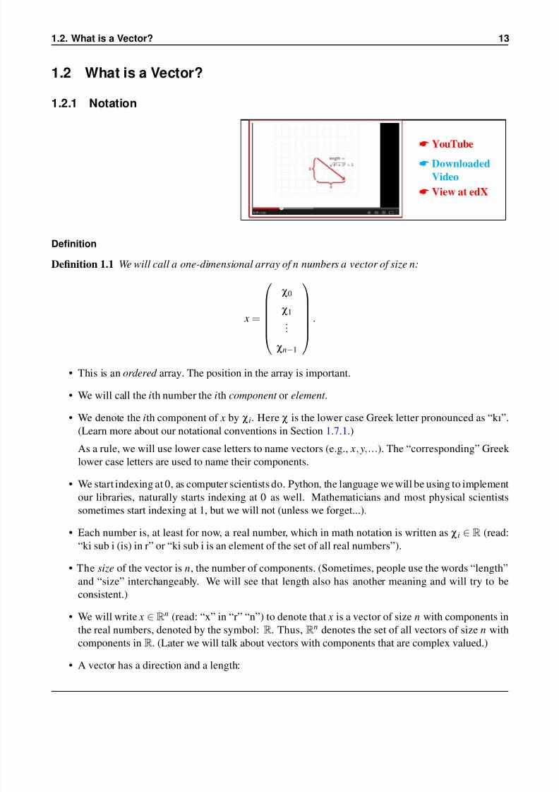
YouTube
Downloaded
Video
View at edX
Definition
Definition 1.1 We will call a one-dimensional array of n numbers a vector of size n:
x =
χ0
χ1
...
χn−1
.
• This is an ordered array. The position in the array is important.
• We will call the ith number the ith component or element .
• We denote the ith component of x by χi. Here χ is the lower case Greek letter pronounced as “kı”.(Learn more about our notational conventions in Section 1.7.1.)
As a rule, we will use lower case letters to name vectors (e.g., x, y,...). The “corresponding” Greek
lower case letters are used to name their components.
• We start indexing at 0, as computer scientists do. Python, the language we will be using to implement
our libraries, naturally starts indexing at 0 as well. Mathematicians and most physical scientists
sometimes start indexing at 1, but we will not (unless we forget...).
• Each number is, at least for now, a real number, which in math notation is written as χi ∈ R (read:
“ki sub i (is) in r” or “ki sub i is an element of the set of all real numbers”).
• The size of the vector is n, the number of components. (Sometimes, people use the words “length”
and “size” interchangeably. We will see that length also has another meaning and will try to be
consistent.)
• We will write x ∈ Rn (read: “x” in “r” “n”) to denote that x is a vector of size n with components in
the real numbers, denoted by the symbol: R. Thus, Rn denotes the set of all vectors of size n with
components in R. (Later we will talk about vectors with components that are complex valued.)
• A vector has a direction and a length:
7/18/2019 Week1
http://slidepdf.com/reader/full/week1-56d46b8915d3b 7/53
Week 1. Vectors in Linear Algebra 14
– Its direction is often visualized by drawing an arrow from the origin to the point (χ0,χ1, . . . ,χn−1),
but the arrow does not necessarily need to start at the origin.
– Its length is given by the Euclidean length of this arrow,
χ2
0 +χ21 + · · ·+χ2
n−1,
It is denoted by x2 called the two-norm. Some people also call this the magnitude of the
vector.
• A vector does not have a location. Sometimes we will show it starting at the origin, but that is only
for convenience. It will often be more convenient to locate it elsewhere or to move it.
Examples
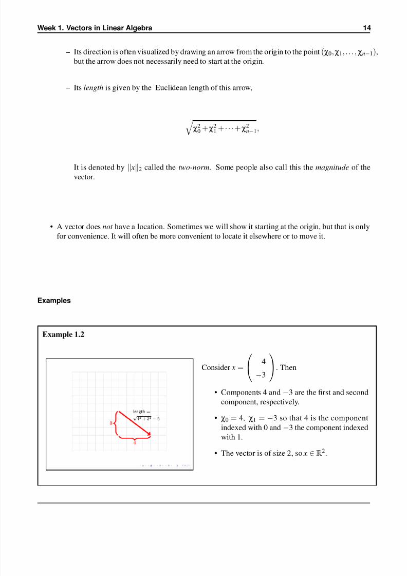
Example 1.2
Consider x =
4
−3
. Then
• Components 4 and −3 are the first and second
component, respectively.
• χ0 = 4, χ1 = −3 so that 4 is the component
indexed with 0 and −3 the component indexed
with 1.
• The vector is of size 2, so x ∈ R2.
7/18/2019 Week1
http://slidepdf.com/reader/full/week1-56d46b8915d3b 8/53
1.2. What is a Vector? 15
Exercises
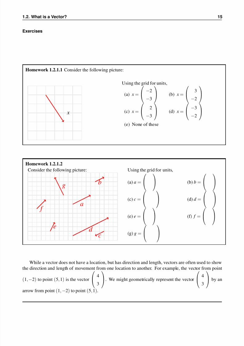
Homework 1.2.1.1 Consider the following picture:
x
Using the grid for units,
(a) x =
−2
−3
(b) x =
3
−2
(c) x =
2
−3
(d) x =
−3
−2
(e) None of these
Homework 1.2.1.2
Consider the following picture:
a
b
cd
e
f
g
Using the grid for units,
(a) a =
(b) b =
(c) c =
(d) d =
(e) e =
(f) f =
(g) g =
While a vector does not have a location, but has direction and length, vectors are often used to show
the direction and length of movement from one location to another. For example, the vector from point
(1,−2) to point (5,1) is the vector
4
3
. We might geometrically represent the vector
4
3
by an
arrow from point (1,−2) to point (5,1).

7/18/2019 Week1
http://slidepdf.com/reader/full/week1-56d46b8915d3b 9/53
Week 1. Vectors in Linear Algebra 16
Homework 1.2.1.3 Write each of the following as a vector:
• The vector represented geometrically in R2 by an arrow from point (−1,2) to point (0,0).
• The vector represented geometrically in R2 by an arrow from point (0,0) to point (−1,2).
• The vector represented geometrically in R3 by an arrow from point (−1,2,4) to point
(0,0,1).
• The vector represented geometrically in R3 by an arrow from point (1,0,0) to point
(4,2,−1).
1.2.2 Unit Basis Vectors
YouTube
Downloaded
Video
View at edX
Definition
Definition 1.3 An important set of vectors is the set of unit basis vectors given by
e j =
0...
0
1
0...
0
j zeroes
←− component indexed by j
n− j−1 zeroes
where the “1” appears as the component indexed by j. Thus, we get the set {e0,e1, . . . ,en−1} ⊂ Rn givenby
e0 =
1
0...
0
0
, e1 =
0
1...
0
0
, · · · , en−1 =
0
0...
0
1
.

7/18/2019 Week1
http://slidepdf.com/reader/full/week1-56d46b8915d3b 10/53
1.3. Simple Vector Operations 17
In our presentations, any time you encounter the symbol e j, it always refers to the unit basis vector with
the “1” in the component indexed by j.
These vectors are also referred to as the standard basis vectors. Other terms used for these vectors
are natural basis and canonical basis. Indeed, “unit basis vector” appears to be less commonly used.
But we will use it anyway!
Homework 1.2.2.1 Which of the following is not a unit basis vector?
(a)
0
0
1
0
(b)
0
1
(c)
√ 2
2√ 2
2
(d)
1
0
0
(e) None of these are unit
basis vectors.
1.3 Simple Vector Operations
1.3.1 Equality (=), Assignment (:=), and Copy
YouTube
DownloadedVideo
View at edX
Definition
Definition 1.4 Two vectors x, y ∈ Rn are equal if all their components are element-wise equal:
x = y if and only if χi = ψ i , for all 0 ≤ i < n.
This means that two vectors are equal if they point in the same direction and are of the same length.
They don’t, however, need to have the same location.
The assignment or copy operation assigns the content of one vector to another vector. In our mathe-
matical notation, we will denote this by the symbol := (pronounce: becomes). After the assignment, the
two vectors are equal to each other.

7/18/2019 Week1
http://slidepdf.com/reader/full/week1-56d46b8915d3b 11/53
Week 1. Vectors in Linear Algebra 18
Algorithm
The following algorithm copies vector x ∈ Rn into vector y ∈ R
n, performing the operation y := x:
ψ 0
ψ 1...
ψ n−1
:=
χ0
χ1...
χn−1
for i = 0, . . . ,n−1
ψ i := χi
endfor
Cost
(Notice: we will cost of various operations in more detail in the future.)
Copying one vector to another vector requires 2n memory operations (memops).
• The vector x of length n must be read, requiring n memops and
• the vector y must be written, which accounts for the other n memops.
Homework 1.3.1.1 Decide if the two vectors are equal.
• The vector represented geometrically in R2 by an arrow from point (−1,2) to point (0,0)and the vector represented geometrically in R2 by an arrow from point (1,−2) to point
(2,−1) are equal.
True/False
• The vector represented geometrically in R3 by an arrow from point (1,−1,2) to point
(0,0,0) and the vector represented geometrically in R3 by an arrow from point (1,1,−2)
to point (0,2,−4) are equal.
True/False
1.3.2 Vector Addition (AD D)
YouTube
Downloaded
Video
View at edX

7/18/2019 Week1
http://slidepdf.com/reader/full/week1-56d46b8915d3b 12/53
1.3. Simple Vector Operations 19
Definition
Definition 1.5 Vector addition x + y (sum of vectors) is defined by
x + y =
χ0
χ1
...
χn−1
+
ψ 0
ψ 1...
ψ n−1
=
χ0 +ψ 0
χ1 +ψ 1...
χn−1 +ψ n−1
.
In other words, the vectors are added element-wise, yielding a new vector of the same size.
Exercises
Homework 1.3.2.1 −1
2
+ −3
−2
=
Homework 1.3.2.2
−3
−2
+
−1
2
=
Homework 1.3.2.3 For x, y ∈ Rn,
x + y = y + x.
Always/Sometimes/Never
Homework 1.3.2.4
−1
2
+
−3
−2
+
1
2
=
Homework 1.3.2.5
−1
2
+
−3
−2
+
1
2
=
Homework 1.3.2.6 For x, y, z ∈ Rn, ( x + y) + z = x + ( y + z). Always/Sometimes/Never
Homework 1.3.2.7
−1
2
+
0
0
=
Homework 1.3.2.8 For x ∈ Rn, x + 0 = x, where 0 is the zero vector of appropriate size.
Always/Sometimes/Never
7/18/2019 Week1
http://slidepdf.com/reader/full/week1-56d46b8915d3b 13/53
Week 1. Vectors in Linear Algebra 20
Algorithm
The following algorithm assigns the sum of vectors x and y (of size n and stored in arrays x and y) to
vector z (of size n and stored in array z), computing z := x + y:
ζ0
ζ1
...
ζn−1
:=
χ0 +ψ 0
χ1 +ψ 1...
χn−1 +ψ n−1
.
for i = 0, . . . ,n−1
ζi := χi +ψ i
endfor
Cost
On a computer, real numbers are stored as floating point numbers, and real arithmetic is approximated with
floating point arithmetic. Thus, we count floating point operations (flops): a multiplication or addition each
cost one flop.
Vector addition requires 3n memops ( x is read, y is read, and the resulting vector is written) and n flops
(floating point additions).
For those who understand “Big-O” notation, the cost of the SCAL operation, which is seen in the next
section, is O(n). However, we tend to want to be more exact than just saying O(n). To us, the coefficient
in front of n is important.
Vector addition in sports
View the following video and find out how the “parallelogram method” for vector addition is useful in
sports:
http://www.scientificamerican.com/article.cfm?id=football-vectors
Discussion: Can you find other examples of how vector addition is used in sports?
1.3.3 Scaling (SCAL)
YouTube
Downloaded
Video
View at edX
7/18/2019 Week1
http://slidepdf.com/reader/full/week1-56d46b8915d3b 14/53
1.3. Simple Vector Operations 21
Definition
Definition 1.6 Multiplying vector x by scalar α yields a new vector, α x, in the same direction as x, but
scaled by a factor α. Scaling a vector by α means each of its components, χi , is multiplied by α:
α x = α
χ0
χ1
...
χn−1
=
αχ0
αχ1
...
αχn−1
.
Exercises
Homework 1.3.3.1
−1
2
+
−1
2
+
−1
2
=
Homework 1.3.3.2 3
−1
2
=
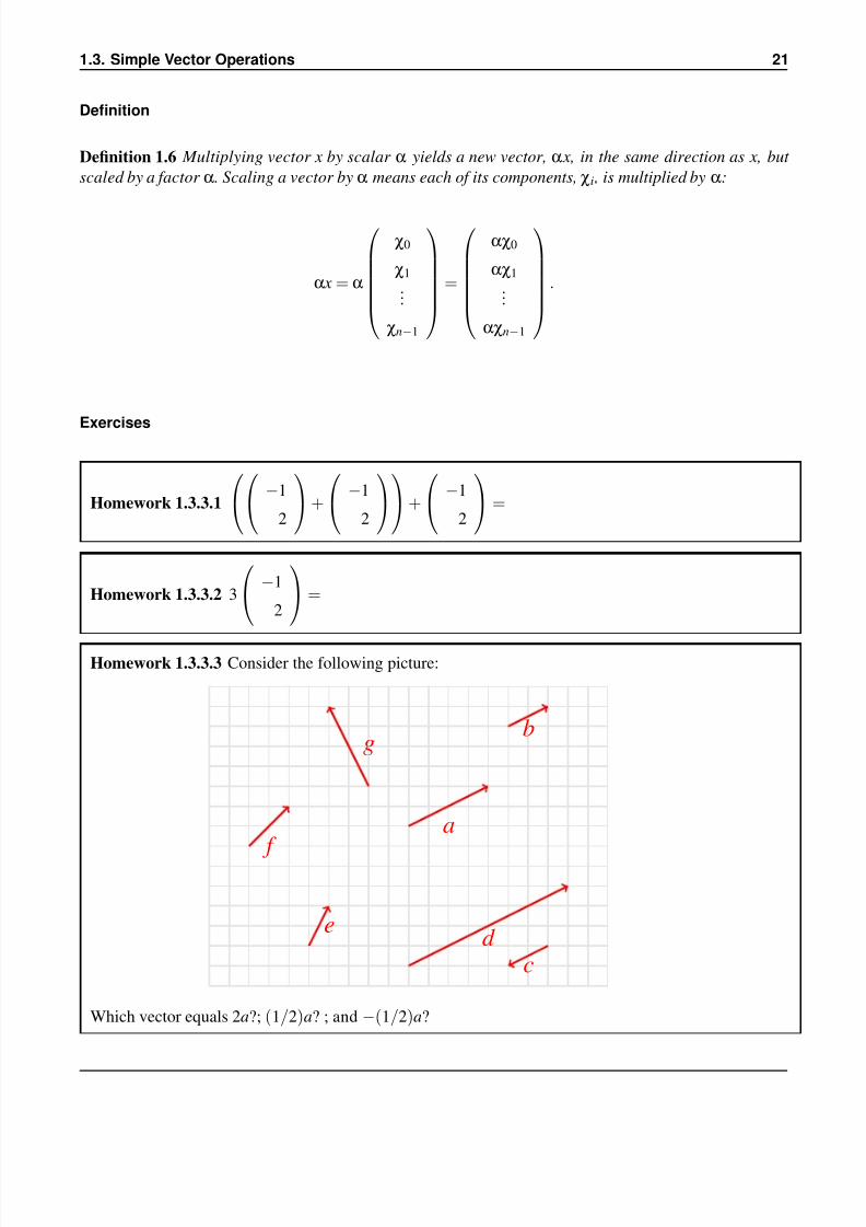
Homework 1.3.3.3 Consider the following picture:
a
b
cd
e
f
g
Which vector equals 2a?; (1/2)a? ; and −(1/2)a?
7/18/2019 Week1
http://slidepdf.com/reader/full/week1-56d46b8915d3b 15/53
Week 1. Vectors in Linear Algebra 22
Algorithm
The following algorithm scales a vector x ∈ Rn by α, overwriting x with the result α x:
χ0
χ1...
χn−1
:=
αχ0
αχ1...
αχn−1
.
for i = 0, . . . ,n−1
χi := αχi
endfor
Cost
Scaling a vector requires n flops and 2n + 1 memops. Here, α is only brought in from memory once
and kept in a register for reuse. To fully understand this, you need to know a little bit about computer
architecture.
“Among friends” we will simply say that the cost is 2n memops since the one extra memory operation
(to bring α in from memory) is negligible.
1.3.4 Vector Subtraction
YouTube
Downloaded
Video
View at edX
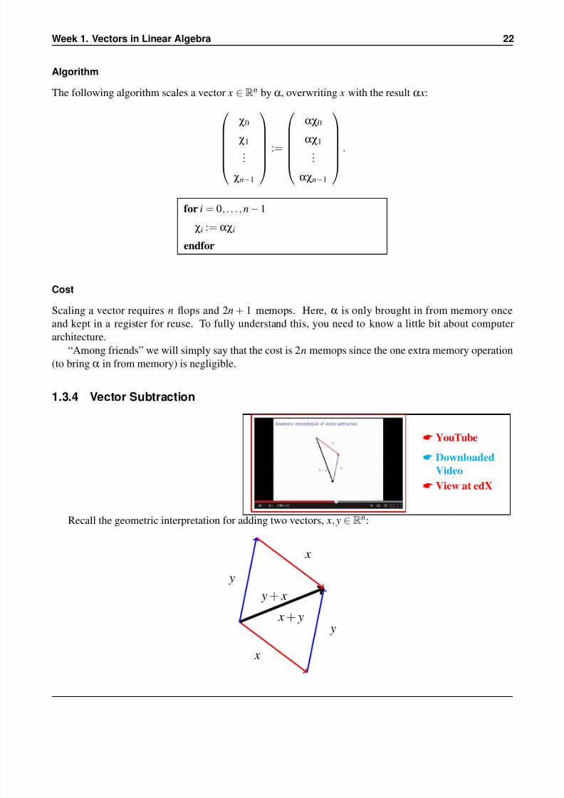
Recall the geometric interpretation for adding two vectors, x, y ∈ Rn:
x
y x + y
y x
y + x

7/18/2019 Week1
http://slidepdf.com/reader/full/week1-56d46b8915d3b 16/53
1.3. Simple Vector Operations 23
Subtracting y from x is defined as
x− y = x + (− y).
We learned in the last unit that − y is the same as (−1) y which is the same as pointing y in the opposite
direction, while keeping it’s length the same. This allows us to take the parallelogram that we used to
illustrate vector addition
x
y
x
y
and change it into the equivalent picture
x
− y
x
− y
Since we know how to add two vectors, we can now illustrate x + (− y):
x
− y
x
− y
x+(− y)
Which then means that x− y can be illustrated by

7/18/2019 Week1
http://slidepdf.com/reader/full/week1-56d46b8915d3b 17/53
Week 1. Vectors in Linear Algebra 24
x
y
x
y
x− y
Finally, we note that the parallelogram can be used to simulaneously illustrate vector addition and sub-
traction:
x
y
x
y
x− y
x + y
(Obviously, you need to be careful to point the vectors in the right direction.)
Now computing x− y when x, y ∈ Rn is a simple matter of subtracting components of y off the corre-
sponding components of x:
x− y =
χ0
χ1
...
χn−1
−
ψ 0
ψ 1...
ψ n−1
=
χ0−ψ 0
χ1−ψ 1...
χn−1−ψ n−1
.
Homework 1.3.4.1 For x ∈ Rn, x− x = 0.
Always/Sometimes/Never
Homework 1.3.4.2 For x, y ∈ Rn, x− y = y− x.
Always/Sometimes/Never
7/18/2019 Week1
http://slidepdf.com/reader/full/week1-56d46b8915d3b 18/53
1.4. Advanced Vector Operations 25
1.4 Advanced Vector Operations
1.4.1 Scaled Vector Addition (AXPY)
YouTube
Downloaded
Video
View at edX
Definition
Definition 1.7 One of the most commonly encountered operations when implementing more complex lin-ear algebra operations is the scaled vector addition, which (given x, y ∈ R
n) computes y := α x + y:
α x + y = α
χ0
χ1
...
χn−1
+
ψ 0
ψ 1...
ψ n−1
=
αχ0 +ψ 0
αχ1 +ψ 1...
αχn−1 +ψ n−1
.
It is often referred to as the AXPY operation, which stands for alpha times x plus y. We emphasize that it
is typically used in situations where the output vector overwrites the input vector y.
Algorithm
Obviously, one could copy x into another vector, scale it by α, and then add it to y. Usually, however,
vector y is simply updated one element at a time:
ψ 0
ψ 1
...
ψ n−1
:=
αχ0 +ψ 0
αχ1 +ψ 1
...
αχn−1 +ψ n−1
.
for i = 0, . . . ,n−1
ψ i := αχi +ψ i
endfor

7/18/2019 Week1
http://slidepdf.com/reader/full/week1-56d46b8915d3b 19/53
Week 1. Vectors in Linear Algebra 26
Cost
In Section 1.3 for many of the operations we discuss the cost in terms of memory operations (memops)
and floating point operations (flops). This is discussed in the text, but not the videos. The reason for this is
that we will talk about the cost of various operations later in a larger context, and include these discussions
here more for completely.
Homework 1.4.1.1 What is the cost of an axpy operation?
• How many memops?
• How many flops?
1.4.2 Linear Combinations of Vectors
YouTube
Downloaded
Video
View at edX
Discussion
There are few concepts in linear algebra more fundamental than linear combination of vectors.
Definition
Definition 1.8 Let u,v ∈ Rm and α,β ∈ R. Then αu +βv is said to be a linear combination of vectors u
and v:
αu +βv = α
υ0
υ1
...
υm
−1
+β
ν0
ν1
...
νm
−1
=
αυ0
αυ1
...
αυm
−1
+
βν0
βν1
...
βνm
−1
=
αυ0 +βν0
αυ1 +βν1
...
αυm
−1 +βνm
−1
.
The scalars α and β are the coefficients used in the linear combination.
More generally, if v0, . . . ,vn−1 ∈ Rm are n vectors and χ0, . . . ,χn−1 ∈ R are n scalars, then χ0v0 +
χ1v1 + · · ·+χn−1vn−1 is a linear combination of the vectors, with coefficients χ0, . . . ,χn−1.
We will often use the summation notation to more concisely write such a linear combination:
χ0v0 +χ1v1 + · · ·+χn−1vn−1 =n−1
∑ j=0
χ jv j.

7/18/2019 Week1
http://slidepdf.com/reader/full/week1-56d46b8915d3b 20/53
1.4. Advanced Vector Operations 27
Homework 1.4.2.1
3
2
4
−1
0
+ 2
1
0
1
0
=
Homework 1.4.2.2
−3
1
0
0
+ 2
0
1
0
+ 4
0
0
1
=
Homework 1.4.2.3 Find α, β, γ such that
α
1
0
0
+β
0
1
0
+ γ
0
0
1
=
2
−1
3
α = β = γ =
Algorithm
Given v0, . . . ,vn−1 ∈ Rm and χ0, . . . ,χn−1 ∈ R the linear combination w = χ0v0 +χ1v1 + · · ·+χn−1vn−1
can be computed by first setting the result vector w to the zero vector of size n, and then performing n
AXPY operations:
w = 0 (the zero vector of size m)
for j = 0, . . . ,n−1
w := χ jv j + w
endfor
The axpy operation computed y := α x + y. In our algorithm, χ j takes the place of α, v j the place of x, and
w the place of y.
Cost
We noted that computing w =χ0v0 +χ1v1 + · · ·χn−1vn−1 can be implementated as n AXPY operations. This
suggests that the cost is n times the cost of an AXPY operation with vectors of size m: n× (2m) = 2mn
flops and (approximately) n× (3m) memops.
7/18/2019 Week1
http://slidepdf.com/reader/full/week1-56d46b8915d3b 21/53
Week 1. Vectors in Linear Algebra 28
However, one can actually do better. The vector w is updated repeatedly. If this vector stays in the
L1 cache of a computer, then it needs not be repeatedly loaded from memory, and the cost becomes m
memops (to load w into the cache) and then for each AXPY operation (approximately) m memops (to read
v j (ignoring the cost of reading χ j). Then, once w has been completely updated, it can be written back
to memory. So, the total cost related to accessing memory becomes m + n×m + m = (n + 2)m ≈ mn
memops.
An important example
Example 1.9 Given any x ∈ Rn with x =
χ0
χ1
...
χn−1
, this vector can always be written as the
linear combination of the unit basis vectors given by
x =
χ0
χ1
...
χn−1
= χ0
1
0...
0
0
+χ1
0
1...
0
0
+ · · ·+χn−1
0
0...
0
1
= χ0e0 +χ1e1 + · · ·+χn−1en−1 =n−1
∑i=0
χiei.
Shortly, this will become really important as we make the connection between linear combina-
tions of vectors, linear transformations, and matrices.
1.4.3 Dot or Inner Product (DOT)
YouTube
Downloaded
Video
View at edX

7/18/2019 Week1
http://slidepdf.com/reader/full/week1-56d46b8915d3b 22/53
1.4. Advanced Vector Operations 29
Definition
The other commonly encountered operation is the dot (inner) product. It is defined by
dot( x, y) =n−1
∑i=0
χiψ i = χ0ψ 0 +χ1ψ 1 +· · ·
+χn
−1ψ n
−1.
Alternative notation
We will often write
xT y = dot( x, y) =
χ0
χ1
...
χn−1
T
ψ 0
ψ 1...
ψ n−1
= χ0 χ1 · · · χn−1
ψ 0
ψ 1...
ψ n−1
= χ0ψ 0 +χ1ψ 1 + · · ·+χn−1ψ n−1
for reasons that will become clear later in the course.
Exercises
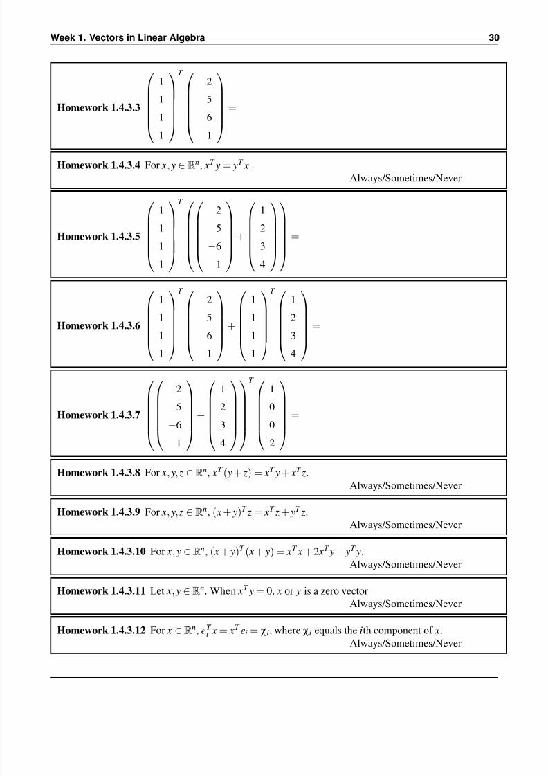
Homework 1.4.3.1
2
5
−6
1
T
1
1
1
1
1
1
=
Homework 1.4.3.2
2
5
−6
1
T
1
1
1
1
=
7/18/2019 Week1
http://slidepdf.com/reader/full/week1-56d46b8915d3b 23/53
Week 1. Vectors in Linear Algebra 30
Homework 1.4.3.3
1
1
1
1
T
2
5
−6
1
=
Homework 1.4.3.4 For x, y ∈ Rn, xT y = yT x.
Always/Sometimes/Never
Homework 1.4.3.5
1
1
1
1
T
2
5
−6
1
+
1
2
3
4
=
Homework 1.4.3.6
1
1
1
1
T
2
5
−6
1
+
1
1
1
1
T
1
2
3
4
=
Homework 1.4.3.7
2
5
−6
1
+
1
2
3
4
T
1
0
0
2
=
Homework 1.4.3.8 For x, y, z ∈ Rn, xT ( y + z) = xT y + xT z.
Always/Sometimes/Never
Homework 1.4.3.9 For x, y, z ∈ Rn, ( x + y)T z = xT z + yT z.
Always/Sometimes/Never
Homework 1.4.3.10 For x, y ∈ Rn, ( x + y)T ( x + y) = xT x + 2 xT y + yT y.
Always/Sometimes/Never
Homework 1.4.3.11 Let x, y ∈ Rn. When xT y = 0, x or y is a zero vector.
Always/Sometimes/Never
Homework 1.4.3.12 For x ∈ Rn, eT
i x = xT ei = χi, where χi equals the ith component of x.
Always/Sometimes/Never
7/18/2019 Week1
http://slidepdf.com/reader/full/week1-56d46b8915d3b 24/53
1.4. Advanced Vector Operations 31
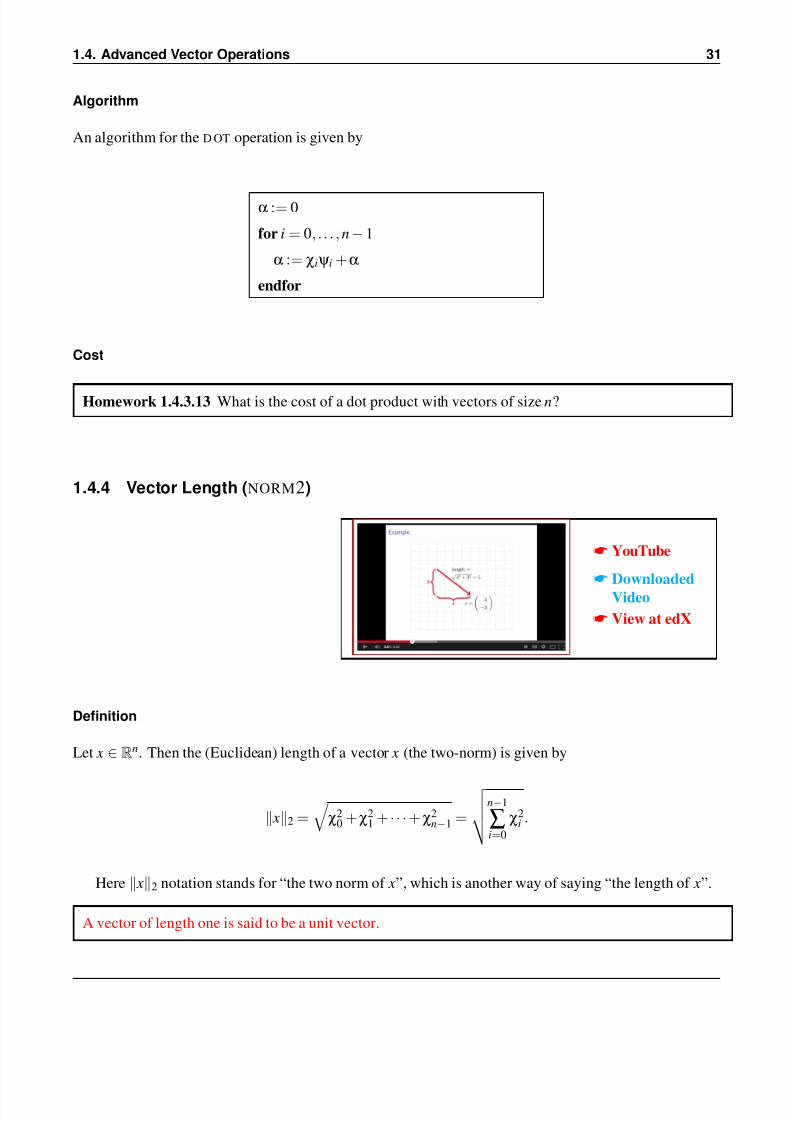
Algorithm
An algorithm for the D OT operation is given by
α := 0
for i = 0, . . . ,n−1
α := χiψ i +α
endfor
Cost
Homework 1.4.3.13 What is the cost of a dot product with vectors of size n?
1.4.4 Vector Length (NORM2)
YouTube
Downloaded
Video
View at edX
Definition
Let x ∈ Rn. Then the (Euclidean) length of a vector x (the two-norm) is given by
x2 = χ2
0 +χ21 + · · ·+χ2
n−1 =
n−1
∑i=0
χ2i .
Here x2 notation stands for “the two norm of x”, which is another way of saying “the length of x”.
A vector of length one is said to be a unit vector.

7/18/2019 Week1
http://slidepdf.com/reader/full/week1-56d46b8915d3b 25/53
Week 1. Vectors in Linear Algebra 32
Exercises
Homework 1.4.4.1 Compute the lengths of the following vectors:
(a)
0
0
0
(b)
1/21/2
1/2
1/2
(c)
1
−2
2
(d)
0
0
1
0
0
Homework 1.4.4.2 Let x ∈ Rn. The length of x is less than zero: x2 < 0.
Always/Sometimes/Never
Homework 1.4.4.3 If x is a unit vector then x is a unit basis vector.
TRUE/FALSE
Homework 1.4.4.4 If x is a unit basis vector then x is a unit vector.
TRUE/FALSE
Homework 1.4.4.5 If x and y are perpendicular (orthogonal) then xT y = 0.
TRUE/FALSE
Hint: Consider the picture
x y
x + y
Homework 1.4.4.6 Let x, y ∈ Rn be nonzero vectors and let the angle between them equal θ.
Then
cosθ = xT y
x2 y2.
Always/Sometimes/Never
Hint: Consider the picture and the “Law of Cosines” that you learned in high school. (Or look up this law!)
x
y θ
y− x

7/18/2019 Week1
http://slidepdf.com/reader/full/week1-56d46b8915d3b 26/53
1.4. Advanced Vector Operations 33
Homework 1.4.4.7 Let x, y ∈ Rn be nonzero vectors. Then xT y = 0 if and only if x and y are
orthogonal (perpendicular).
True/False
Algorithm
Clearly, x2 =√
xT x, so that the D OT operation can be used to compute this length.
Cost
If computed with a dot product, it requires approximately n memops and 2n flops.
1.4.5 Vector Functions
YouTube
Downloaded
Video
View at edX
Last week, we saw a number of examples where a function, f , takes in one or more scalars and/or
vectors, and outputs a vector (where a scalar can be thought of as a special case of a vector, with unit size).
These are all examples of vector-valued functions (or vector functions for short).
Definition
A vector(-valued) function is a mathematical functions of one or more scalars and/or vectors whose output
is a vector.
Examples
Example 1.10
f (α,β) =
α+β
α−β
so that f (−2,1) =
−2 + 1
−2
−1
=
−1
−3
.
Example 1.11
f (α,
χ0
χ1
χ2
) =
χ0 +α
χ1 +α
χ2 +α
so that f (−2,
1
2
3
) =
1 + (−2)
2 + (−2)
3 + (−2)
=
−1
0
1
.
Example 1.12 The AXPY and D OT vector functions are other functions that we have already encountered.

7/18/2019 Week1
http://slidepdf.com/reader/full/week1-56d46b8915d3b 27/53
Week 1. Vectors in Linear Algebra 34
Example 1.13
f (α,
χ0
χ1
χ2
) =
χ0 +χ1
χ1 +χ2
so that f (
1
2
3
) =
1 + 2
2 + 3
=
3
5
.
7/18/2019 Week1
http://slidepdf.com/reader/full/week1-56d46b8915d3b 28/53
1.4. Advanced Vector Operations 35
Exercises
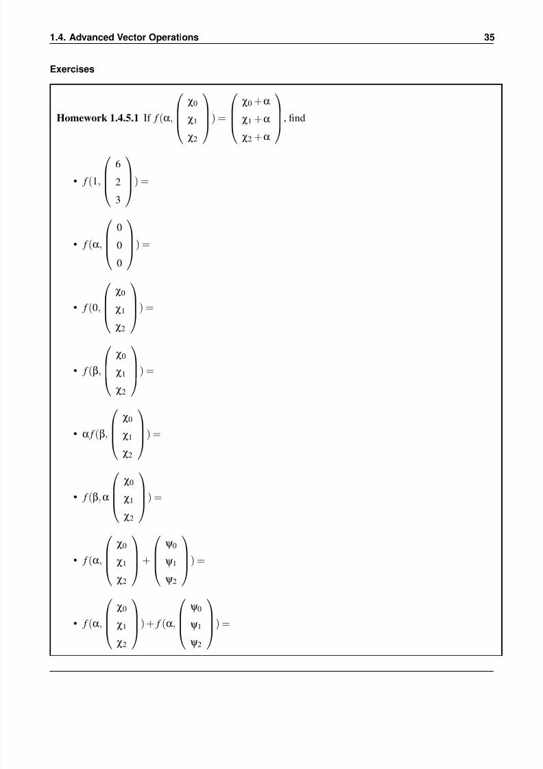
Homework 1.4.5.1 If f (α,
χ0
χ1
χ2
) =
χ0 +α
χ1 +α
χ2 +α
, find
• f (1,
6
2
3
) =
• f (α,
0
0
0
) =
• f (0,
χ0
χ1
χ2
) =
• f (β,
χ0
χ1
χ2
) =
• α f (β,
χ0
χ1
χ2
) =
• f (β,α
χ0
χ1
χ2
) =
• f (α,
χ0
χ1
χ2
+
ψ 0
ψ 1
ψ 2
) =
• f (α,
χ0
χ1
χ2
) + f (α,
ψ 0
ψ 1
ψ 2
) =

7/18/2019 Week1
http://slidepdf.com/reader/full/week1-56d46b8915d3b 29/53
Week 1. Vectors in Linear Algebra 36
1.4.6 Vector Functions that Map a Vector to a Vector
YouTube
DownloadedVideo
View at edX
Now, we can talk about such functions in general as being a function from one vector to another vector.
After all, we can take all inputs, make one vector with the separate inputs as the elements or subvectors of
that vector, and make that the input for a new function that has the same net effect.
Example 1.14 Instead of
f (α,β) =
α+β
α−β
so that f (−2,1) =
−2 + 1
−2−1
=
−1
−3
we can define
g(
α
β
) =
α+β
α−β
so that g(
−2
1
) =
−2 + 1
−2−1
=
−1
−3
Example 1.15 Instead of
f (α,
χ0
χ1
χ2
) =
χ0 +α
χ1 +α
χ2 +α
so that f (−2,
1
2
3
) =
1 + (−2)
2 + (−2)
3 + (−2)
=
−1
0
1
,
we can define
g(
α
χ0
χ1
χ2
) = g(
α
χ0
χ1
χ2
) =
χ0 +αχ1 +α
χ2 +α
so that g(
−
2
1
2
3
) =
1 + (−2)2 + (−2)
3 + (−2)
=
−1
0
1
.
The bottom line is that we can focus on vector functions that map a vector of size n into a vector of
size m, which is written as
f : Rn → Rm.

7/18/2019 Week1
http://slidepdf.com/reader/full/week1-56d46b8915d3b 30/53
1.4. Advanced Vector Operations 37
Exercises
Homework 1.4.6.1 If f (
χ0
χ1
χ2
) =
χ0 + 1
χ1 + 2
χ2 + 3
, evaluate
• f (
6
2
3
) =
• f (
0
0
0
) =
• f (2
χ0
χ1
χ2
) =
• 2 f (
χ0
χ1
χ2
) =
• f (α
χ0
χ1
χ2
) =
• α f (
χ0
χ1
χ2
) =
• f (
χ0
χ1
χ2
+
ψ 0
ψ 1
ψ 2
) =
• f (
χ0
χ1
χ2
) + f (
ψ 0
ψ 1
ψ 2
) =

7/18/2019 Week1
http://slidepdf.com/reader/full/week1-56d46b8915d3b 31/53
Week 1. Vectors in Linear Algebra 38
Homework 1.4.6.2 If f (
χ0
χ1
χ2
) =
χ0
χ0 +χ1
χ0 +
χ1 +
χ2
, evaluate
• f (
6
2
3
) =
• f (
0
0
0
) =
• f (2
χ0
χ1
χ2
) =
• 2 f (
χ0
χ1
χ2
) =
• f (α
χ0
χ1
χ2
) =
• α f (
χ0
χ1
χ2
) =
• f (
χ0
χ1
χ2
+
ψ 0ψ 1
ψ 2
) =
• f (
χ0
χ1
χ2
) + f (
ψ 0
ψ 1
ψ 2
) =
7/18/2019 Week1
http://slidepdf.com/reader/full/week1-56d46b8915d3b 32/53
1.5. LAFF Package Development: Vectors 39
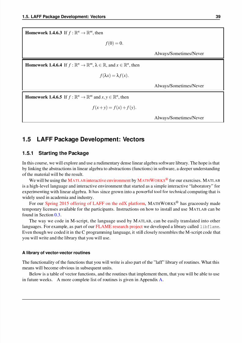
Homework 1.4.6.3 If f : Rn →Rm, then
f (0) = 0.
Always/Sometimes/Never
Homework 1.4.6.4 If f : Rn →Rm, λ ∈ R, and x ∈ R
n, then
f (λ x) = λ f ( x).
Always/Sometimes/Never
Homework 1.4.6.5 If f : Rn →Rm and x, y ∈ R
n, then
f ( x + y) = f ( x) + f ( y).
Always/Sometimes/Never
1.5 LAFF Package Development: Vectors
1.5.1 Starting the Package
In this course, we will explore and use a rudimentary dense linear algebra software library. The hope is that
by linking the abstractions in linear algebra to abstractions (functions) in software, a deeper understanding
of the material will be the result.
We will be using the MATLAB interactive environment by MATHWORKS® for our exercises. MATLAB
is a high-level language and interactive environment that started as a simple interactive “laboratory” for
experimenting with linear algebra. It has since grown into a powerful tool for technical computing that is
widely used in academia and industry.
For our Spring 2015 offering of LAFF on the edX platform, MATHWORKS® has graceously made
temporary licenses available for the participants. Instructions on how to install and use MATLAB can be
found in Section 0.3.
The way we code in M-script, the language used by M ATLAB, can be easily translated into other
languages. For example, as part of our FLAME research project we developed a library called libflame.
Even though we coded it in the C programming language, it still closely resembles the M-script code that
you will write and the library that you will use.
A library of vector-vector routines
The functionality of the functions that you will write is also part of the ”laff” library of routines. What this
means will become obvious in subsequent units.
Below is a table of vector functions, and the routines that implement them, that you will be able to use
in future weeks. A more complete list of routines is given in Appendix A.
7/18/2019 Week1
http://slidepdf.com/reader/full/week1-56d46b8915d3b 33/53
Week 1. Vectors in Linear Algebra 40
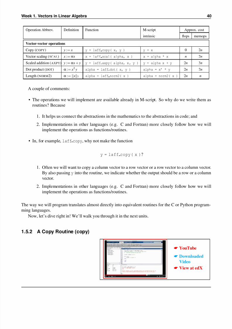
Operation Abbrev. Definition Function M-script Approx. cost
intrinsic flops memops
Vector-vector operations
Copy (COPY) y := x y = laff copy( x, y ) y = x 0 2n
Vector scaling (SCAL) x := α x x = laff scal( alpha, x ) x = alpha * x n 2nScaled addition (AXPY) y := α x + y y = laff axpy( a lpha, x , y ) y = alpha x + y 2n 3n
Dot product (DOT) α := xT y alpha = laff dot( x, y ) alpha = x’ * y 2n 2n
Length (NORM2) α := x2 alpha = laff norm2( x ) alpha = norm2( x ) 2n n
A couple of comments:
• The operations we will implement are available already in M-script. So why do we write them as
routines? Because
1. It helps us connect the abstractions in the mathematics to the abstractions in code; and
2. Implementations in other languages (e.g. C and Fortran) more closely follow how we will
implement the operations as functions/routines.
• In, for example, laff copy, why not make the function
y = laff copy( x )?
1. Often we will want to copy a column vector to a row vector or a row vector to a column vector.
By also passing y into the routine, we indicate whether the output should be a row or a columnvector.
2. Implementations in other languages (e.g. C and Fortran) more closely follow how we will
implement the operations as functions/routines.
The way we will program translates almost directly into equivalent routines for the C or Python program-
ming languages.
Now, let’s dive right in! We’ll walk you through it in the next units.
1.5.2 A Copy Routine (copy)
YouTube
Downloaded
Video
View at edX
7/18/2019 Week1
http://slidepdf.com/reader/full/week1-56d46b8915d3b 34/53
1.5. LAFF Package Development: Vectors 41
Homework 1.5.2.1 Implement the function laff copy that copies a vector into another vector.
The function is defined as
function [ y out ] = laff copy( x, y )
where
• x and y must each be either an n×1 array (column vector) or a 1×n array (row vector);
• y out must be the same kind of vector as y (in other words, if y is a column vector, so is
y out and if y is a row vector, so is y out).
• The function should “transpose” the vector if x and y do not have the same “shape” (if
one is a column vector and the other one is a row vector).
• If x and/or y are not vectors or if the size of (row or column) vector x does not match the
size of (row or column) vector y, the output should be ’FAILED’.
Click for detailed additional instructions.
YouTube
Downloaded
Video
View at edX
1.5.3 A Routine that Scales a Vector (scal)
YouTube
Downloaded
Video
View at edX
7/18/2019 Week1
http://slidepdf.com/reader/full/week1-56d46b8915d3b 35/53
Week 1. Vectors in Linear Algebra 42
Homework 1.5.3.1 Implement the function laff scal that scales a vector x by a scalar α. The
function is defined as
function [ x out ] = laff scal( alpha, x )
where
• x must be either an n×1 array (column vector) or a 1×n array (row vector);
• x out must be the same kind of vector as x; and
• If x or alpha are not a (row or column) vector and scalar, respectively, the output should
be ’FAILED’.
Check your implementation with the script in LAFFSpring2015 -> Code -> laff ->
vecvec -> test scal.m.
1.5.4 A Scaled Vector Addition Routine (axpy)
YouTube
Downloaded
Video
View at edX
Homework 1.5.4.1 Implement the function laff axpy that computes α x + y given scalar αand vectors x and y. The function is defined as
function [ y out ] = laff axpy( alpha, x, y )
where
• x and y must each be either an n
×1 array (column vector) or a 1
×n array (row vector);
• y out must be the same kind of vector as y; and
• If x and/or y are not vectors or if the size of (row or column) vector x does not match the
size of (row or column) vector y, the output should be ’FAILED’.
• If alpha is not a scalar, the output should be ’FAILED’.
Check your implementation with the script in LAFFSpring2015 -> Code -> laff ->
vecvec -> test axpy.m.

7/18/2019 Week1
http://slidepdf.com/reader/full/week1-56d46b8915d3b 36/53
1.5. LAFF Package Development: Vectors 43
1.5.5 An Inner Product Routine (dot)
YouTube
Downloaded
Video
View at edX
Homework 1.5.5.1 Implement the function laff dot that computes the dot product of vectors
x and y. The function is defined as
function [ alpha ] = laff dot( x, y )
where
• x and y must each be either an n×1 array (column vector) or a 1×n array (row vector);
• If x and/or y are not vectors or if the size of (row or column) vector x does not match the
size of (row or column) vector y, the output should be ’FAILED’.
Check your implementation with the script in LAFFSpring2015 -> Code -> laff ->
vecvec -> test dot.m.
1.5.6 A Vector Length Routine (norm2)
YouTube
Downloaded
Video
View at edX
Homework 1.5.6.1 Implement the function laff norm2 that computes the length of vector x.
The function is defined as
function [ alpha ] = laff norm2( x )
where
• x is an n×1 array (column vector) or a 1×n array (row vector);
• If x is not a vector the output should be ’FAILED’.
Check your implementation with the script in LAFFSpring2015 -> Code -> laff ->
vecvec -> test norm2.m.

7/18/2019 Week1
http://slidepdf.com/reader/full/week1-56d46b8915d3b 37/53
Week 1. Vectors in Linear Algebra 44
1.6 Slicing and Dicing
1.6.1 Slicing and Dicing: Dot Product
YouTube
Downloaded
Video
View at edX
In the video, we justify the following theorem:
Theorem 1.16 Let x, y ∈ Rn and partition (Slice and Dice) these vectors as
x =
x0
x1
...
x N −1
and y =
y0
y1
...
y N −1
,
where xi, yi ∈ Rni with ∑ N −1i=0 ni = n. Then
xT y = xT 0 y0 + xT
1 y1 + · · ·+ xT N −1 y N −1 =
N −1
∑i=0
xT i yi.
1.6.2 Algorithms with Slicing and Redicing: Dot Product
YouTube
Downloaded
Video
View at edX

7/18/2019 Week1
http://slidepdf.com/reader/full/week1-56d46b8915d3b 38/53
1.6. Slicing and Dicing 45
Algorithm: [α] := D OT( x, y)
Partition x → xT
x B
, y →
yT
y B
where xT and yT have 0 elements
α := 0
while m( xT ) < m( x) do
Repartition
xT
x B
→
x0
χ1
x2
,
yT
y B
→
y0
ψ 1
y2
whereχ1 has 1 row, ψ 1 has 1 row
α := χ1×ψ 1 +α
Continue with
xT
x B
←
x0
χ1
x2
,
yT
y B
←
y0
ψ 1
y2
endwhile
1.6.3 Coding with Slicing and Redicing: Dot Product
YouTube
Downloaded
Video
View at edX

7/18/2019 Week1
http://slidepdf.com/reader/full/week1-56d46b8915d3b 39/53
Week 1. Vectors in Linear Algebra 46
YouTube
Downloaded
Video
View at edX
Homework 1.6.3.1 Follow along with the video to implement the routine
Dot unb( alpha, x, y ).
The “Spark webpage” can be found at
http://edx-org-utaustinx.s3.amazonaws.com/UT501x/Spark/index.html
or by opening the file
LAFFSpring2015 → Spark → index.html
that should have been in the LAFFSpring2015.zip file you downloaded and unzipped as de-
scribed in Week0 (Unit 0.2.7).
1.6.4 Slicing and Dicing: axpy
YouTube
Downloaded
Video
View at edX
In the video, we justify the following theorem:
Theorem 1.17 Let α ∈ R , x, y ∈ Rn , and partition (Slice and Dice) these vectors as
x =
x0
x1
...
x N −1
and y =
y0
y1
...
y N −1
,

7/18/2019 Week1
http://slidepdf.com/reader/full/week1-56d46b8915d3b 40/53
1.6. Slicing and Dicing 47
where xi, yi ∈ Rni with ∑ N −1
i=0 ni = n. Then
α x + y = α
x0
x1
..
. x N −1
+
y0
y1
..
. y N −1
=
α x0 + y0
α x1 + y1
..
.α x N −1 + y N −1
.
1.6.5 Algorithms with Slicing and Redicing: axpy
YouTube
Downloaded
Video
View at edX
Algorithm: [ y] := A XP Y(α, x, y)
Partition x → xT
x B
, y →
yT
y B
where xT and yT have 0 elements
while m( xT ) < m( x) do
Repartition
xT
x B
→
x0
χ1
x2
,
yT
y B
→
y0
ψ 1
y2
whereχ1 has 1 row, ψ 1 has 1 row
ψ 1 := α×χ1 +ψ 1
Continue with
xT
x B
←
x0
χ1
x2
,
yT
y B
←
y0
ψ 1
y2
endwhile

7/18/2019 Week1
http://slidepdf.com/reader/full/week1-56d46b8915d3b 41/53
Week 1. Vectors in Linear Algebra 48
1.6.6 Coding with Slicing and Redicing: axpy
YouTube
Downloaded
Video
View at edX
Homework 1.6.6.1 Implement the routine
Axpy unb( alpha, x, y ).
The “Spark webpage” can be found at
http://edx-org-utaustinx.s3.amazonaws.com/UT501x/Spark/index.html
or by opening the file
LAFFSpring2015 → Spark → index.html
that should have been in the LAFFSpring2015.zip file you downloaded and unzipped as de-
scribed in Week0 (Unit 0.2.7).
YouTube
Downloaded
Video View at edX
1.7 Enrichment
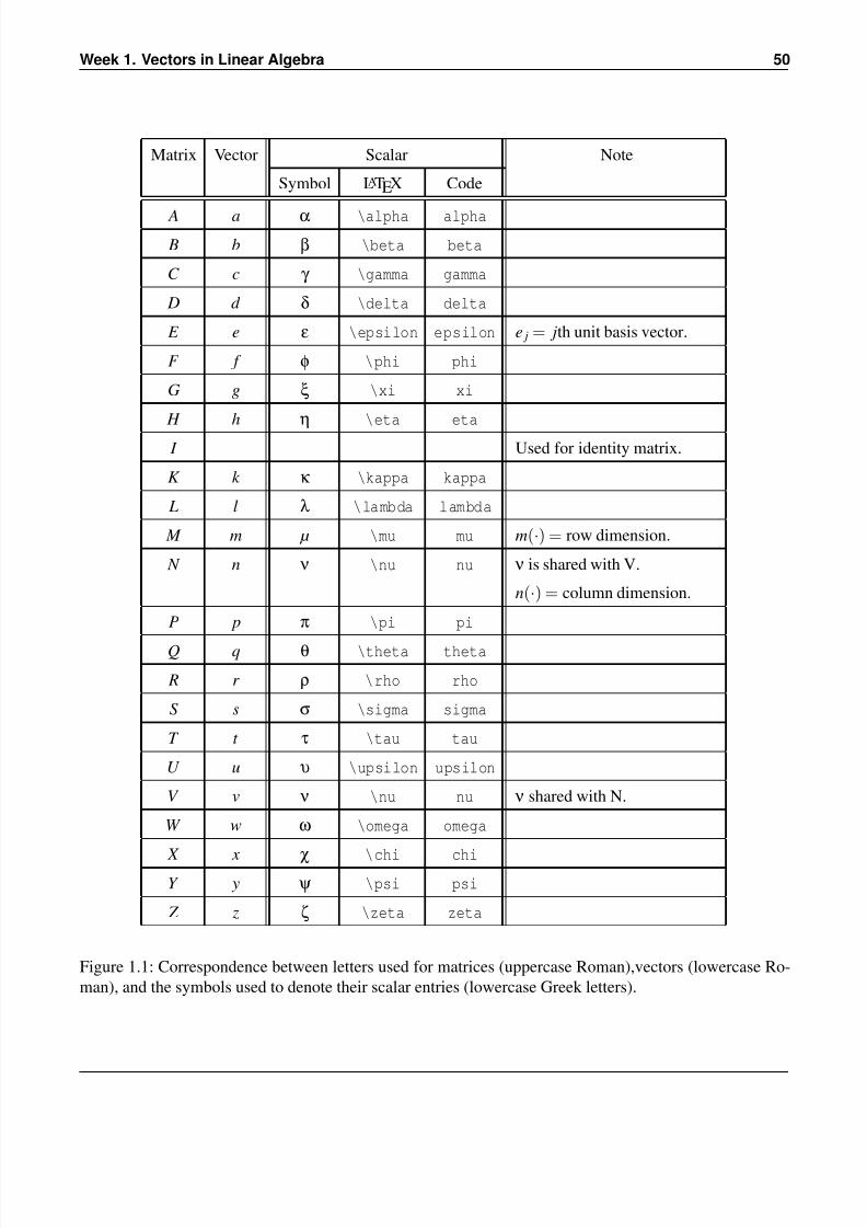
1.7.1 Learn the Greek Alphabet
In this course, we try to use the letters and symbols we use in a very consistent way, to help communication.
As a general rule
• Lowercase Greek letters (α, β, etc.) are used for scalars.
• Lowercase (Roman) letters (a, b, etc) are used for vectors.
• Uppercase (Roman) letters ( A, B, etc) are used for matrices.
Exceptions include the letters i, j, k , l , m, and n, which are typically used for integers.
Typically, if we use a given uppercase letter for a matrix, then we use the corresponding lower case
letter for its columns (which can be thought of as vectors) and the corresponding lower case Greek letter

7/18/2019 Week1
http://slidepdf.com/reader/full/week1-56d46b8915d3b 42/53
1.7. Enrichment 49
for the elements in the matrix. Similarly, as we have already seen in previous sections, if we start with a
given letter to denote a vector, then we use the corresponding lower case Greek letter for its elements.
Table 1.1 lists how we will use the various letters.
1.7.2 Other Norms
A norm is a function, in our case of a vector in Rn, that maps every vector to a nonnegative real number.
The simplest example is the absolute value of a real number: Given α ∈ R, the absolute value of α, often
written as |α|, equals the magnitude of α:
|α| =
α if α ≥ 0
−α otherwise.
Notice that only α = 0 has the property that |α| = 0 and that |α+β| ≤ |α|+ |β|, which is known as the
triangle inequality.
Similarly, one can find functions, called norms, that measure the magnitude of vectors. One exampleis the (Euclidean) length of a vector, which we call the 2-norm: for x ∈ Rn,
x2 =
n−1
∑i=0
χ2i .
Clearly, x2 = 0 if and only if x = 0 (the vector of all zeroes). Also, for x, y ∈ Rn, one can show that
x + y2 ≤ x2 + y2.
A function · : Rn →R is a norm if and only if the following properties hold for all x, y ∈ Rn:
•
x
≥0; and
• x = 0 if and only if x = 0; and
• x + y ≤ x+ y (the triangle inequality).
The 2-norm (Euclidean length) is a norm.
Are there other norms? The answer is yes:
• The taxi-cab norm, also known as the 1-norm:
x1 =n−1
∑i=0
|χi|.
It is sometimes called the taxi-cab norm because it is the distance, in blocks, that a taxi would need
to drive in a city like New York, where the streets are laid out like a grid.
• For 1 ≤ p ≤ ∞, the p-norm:
x p = p
n−1
∑i=0
|χi| p =
n−1
∑i=0
|χi| p1/ p
.
Notice that the 1-norm and the 2-norm are special cases.
7/18/2019 Week1
http://slidepdf.com/reader/full/week1-56d46b8915d3b 43/53
Week 1. Vectors in Linear Algebra 50
Matrix Vector Scalar Note
Symbol LATEX Code
A a α \alpha alpha
B b β \beta beta
C c γ \gamma gamma
D d δ \delta delta
E e ε \epsilon epsilon e j = jth unit basis vector.
F f φ \phi phi
G g ξ \xi xi
H h η \eta eta
I Used for identity matrix.
K k κ \kappa kappa
L l λ \lambda lambda
M m µ \mu mu m(·) = row dimension.
N n ν \nu nu ν is shared with V.
n(·) = column dimension.
P p π \pi pi
Q q θ \theta theta
R r ρ \rho rho
S s σ \sigma sigma
T t τ \tau tau
U u υ \upsilon upsilon
V v ν \nu nu ν shared with N.
W w ω \omega omega
X x χ \chi chiY y ψ \psi psi
Z z ζ \zeta zeta
Figure 1.1: Correspondence between letters used for matrices (uppercase Roman),vectors (lowercase Ro-
man), and the symbols used to denote their scalar entries (lowercase Greek letters).

7/18/2019 Week1
http://slidepdf.com/reader/full/week1-56d46b8915d3b 44/53
1.7. Enrichment 51
• The ∞-norm:
x∞ = lim p→∞
p
n−1
∑i=0
|χi| p = n−1max
i=0|χi|.
The bottom line is that there are many ways of measuring the length of a vector. In this course, we willonly be concerned with the 2-norm.
We will not prove that these are norms, since that, in part, requires one to prove the triangle inequality
and then, in turn, requires a theorem known as the Cauchy-Schwarz inequality. Those interested in seeing
proofs related to the results in this unit are encouraged to investigate norms further.
Example 1.18 The vectors with norm equal to one are often of special interest. Below we plot
the points to which vectors x with x2 = 1 point (when those vectors start at the origin, (0,0)).
(E.g., the vector
1
0
points to the point (1,0) and that vector has 2-norm equal to one, hence
the point is one of the points to be plotted.)
Example 1.19 Similarly, below we plot all points to which vectors x with x1 = 1 point (start-
ing at the origin).
7/18/2019 Week1
http://slidepdf.com/reader/full/week1-56d46b8915d3b 45/53
Week 1. Vectors in Linear Algebra 52
Example 1.20 Similarly, below we plot all points to which vectors x with x∞ = 1 point.
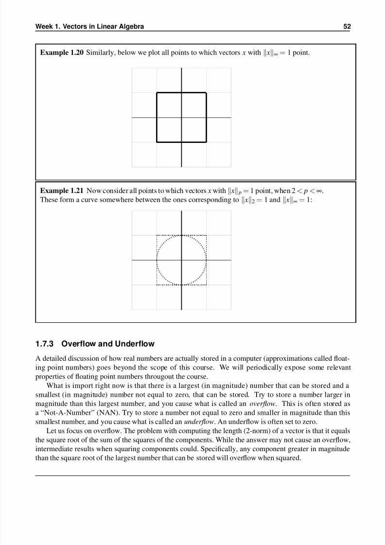
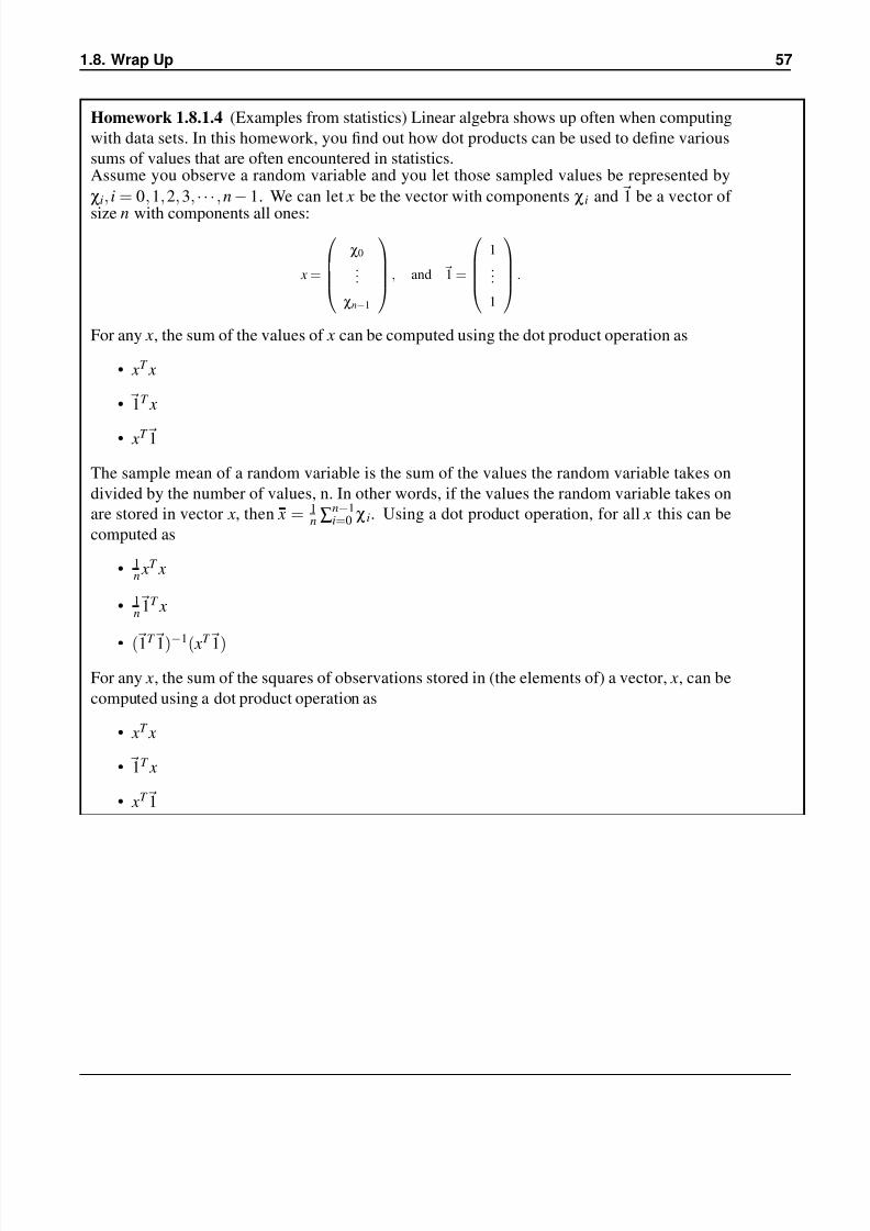
Example 1.21 Now consider all points to which vectors x with x p = 1 point, when 2 < p <∞.These form a curve somewhere between the ones corresponding to x2 = 1 and x∞ = 1:
1.7.3 Overflow and Underflow
A detailed discussion of how real numbers are actually stored in a computer (approximations called float-
ing point numbers) goes beyond the scope of this course. We will periodically expose some relevant
properties of floating point numbers througout the course.
What is import right now is that there is a largest (in magnitude) number that can be stored and a
smallest (in magnitude) number not equal to zero, that can be stored. Try to store a number larger in
magnitude than this largest number, and you cause what is called an overflow. This is often stored as
a “Not-A-Number” (NAN). Try to store a number not equal to zero and smaller in magnitude than this
smallest number, and you cause what is called an underflow. An underflow is often set to zero.
Let us focus on overflow. The problem with computing the length (2-norm) of a vector is that it equals
the square root of the sum of the squares of the components. While the answer may not cause an overflow,
intermediate results when squaring components could. Specifically, any component greater in magnitude
than the square root of the largest number that can be stored will overflow when squared.

7/18/2019 Week1
http://slidepdf.com/reader/full/week1-56d46b8915d3b 46/53
1.7. Enrichment 53
The solution is to exploit the following observation: Let α > 0. Then
x2 =
n−1
∑i=0
χ2i =
n−1
∑i=0
α2χi
α
2
=
α2
n−1
∑i=0
χi
α
2
= α
1
α x
T 1
α x
Now, we can use the following algorithm to compute the length of vector x:
• Choose α = maxn−1i=0 |χi|.
• Scale x := x/α.
• Compute x2 = α√
xT x.
Notice that no overflow for intermediate results (when squaring) will happen because all elements are of
magnitude less than or equal to one. Similarly, only values that are very small relative to the final results
will underflow because at least one of the components of x/α equals one.
1.7.4 A Bit of History
The functions that you developed as part of your LAFF library are very similar in functionality to Fortran
routines known as the (level-1) Basic Linear Algebra Subprograms (BLAS) that are commonly used in
scientific computing libraries. These were first proposed in the 1970s and were used in the development
of one of the first linear algebra libraries, LINPACK. Classic references for that work are
• C. Lawson, R. Hanson, D. Kincaid, and F. Krogh, “Basic Linear Algebra Subprograms for Fortran
Usage,” ACM Transactions on Mathematical Software, 5 (1979) 305–325.
• J. J. Dongarra, J. R. Bunch, C. B. Moler, and G. W. Stewart, LINPACK Users’ Guide, SIAM,
Philadelphia, 1979.
The style of coding that we introduce in Section 1.6 is at the core of our FLAME project and was first
published in
• John A. Gunnels, Fred G. Gustavson, Greg M. Henry, and Robert A. van de Geijn, “FLAME:
Formal Linear Algebra Methods Environment,” ACM Transactions on Mathematical Software, 27
(2001) 422–455.
• Paolo Bientinesi, Enrique S. Quintana-Orti, and Robert A. van de Geijn, “Representing linear alge-
bra algorithms in code: the FLAME application program interfaces,” ACM Transactions on Mathe-
matical Software, 31 (2005) 27–59.

7/18/2019 Week1
http://slidepdf.com/reader/full/week1-56d46b8915d3b 47/53
Week 1. Vectors in Linear Algebra 54
1.8 Wrap Up
1.8.1 Homework
Homework 1.8.1.1 Let
x =
2
−1
, y =
α
β−α
, and x = y.
Indicate which of the following must be true (there may be multiple correct answers):
(a) α = 2
(b) β = (β−α) +α = (−1) + 2 = 1
(c) β−α = −1
(d) β−2 = −1
(e) x = 2e0− e1

7/18/2019 Week1
http://slidepdf.com/reader/full/week1-56d46b8915d3b 48/53
1.8. Wrap Up 55
Homework 1.8.1.2 A displacement vector represents the length and direction of an imaginary,
shortest, straight path between two locations. To illustrate this as well as to emphasize the
difference between ordered pairs that represent positions and vectors, we ask you to map a trip
we made.
In 2012, we went on a journey to share our research in linear algebra. Below are some dis-
placement vectors to describe parts of this journey using longitude and latitude. For exam-ple, we began our trip in Austin, TX and landed in San Jose, CA. Austin has coordinates
30◦ 15 N(orth),97◦ 45 W(est) and San Jose’s are 37◦ 20 N,121◦ 54 W. (Notice that con-
vention is to report first longitude and then latitude.) If we think of using longitude and latitude
as coordinates in a plane where the first coordinate is position E (positive) or W (negative)
and the second coordinate is position N (positive) or S (negative), then Austin’s location is
(−97◦ 45 ,30◦ 15) and San Jose’s are (−121◦ 54,37◦ 20). (Here, notice the switch in the or-
der in which the coordinates are given because we now want to think of E/W as the x coordinate
and N/S as the y coordinate.) For our displacement vector for this, our first component will
correspond to the change in the x coordinate, and the second component will be the change in
the second coordinate. For convenience, we extend the notion of vectors so that the componentsinclude units as well as real numbers. Notice that for convenience, we extend the notion of vec-
tors so that the components include units as well as real numbers (60 minutes ( )= 1 degree(◦).
Hence our displacement vector for Austin to San Jose is
−24◦ 09
7◦ 05
.
After visiting San Jose, we returned to Austin before embarking on a multi-legged excursion.
That is, from Austin we flew to the first city and then from that city to the next, and so forth. In
the end, we returned to Austin.
The following is a table of cities and their coordinates:
City Coordinates City Coordinates
London 00◦ 08 W, 51◦ 30 N Austin −97◦ 45 E, 30◦ 15 N
Pisa 10◦ 21 E, 43◦ 43 N Brussels 04◦ 21 E, 50◦ 51 N
Valencia 00◦ 23 E, 39◦ 28 N Darmstadt 08◦ 39 E, 49◦ 52 N
Zurich 08◦ 33 E, 47◦ 22 N Krakow 19◦ 56 E, 50◦ 4 N
Determine the order in which cities were visited, starting in Austin, given that the legs of the
trip (given in order) had the following displacement vectors:
102◦ 0620◦ 36
→ 04◦ 18−00◦ 59
→ −00◦ 06−02◦ 30
→ 01◦ 48−03◦ 39
→
09◦ 35
06◦ 21
→
−20◦ 04
01◦ 26
→
00◦ 31
−12◦ 02
→
−98◦ 08
−09◦ 13

7/18/2019 Week1
http://slidepdf.com/reader/full/week1-56d46b8915d3b 49/53
Week 1. Vectors in Linear Algebra 56
Homework 1.8.1.3 These days, high performance computers are called clusters and consist
of many compute nodes, connected via a communication network. Each node of the cluster
is basically equipped with a central processing unit (CPU), memory chips, a hard disk, and a
network card. The nodes can be monitored for average power consumption (via power sensors)
and application activity.
A system administrator monitors the power consumption of a node of such a cluster for anapplication that executes for two hours. This yields the following data:
Component Average power (W) Time in use (in hours) Fraction of time in use
CPU 90 1.4 0.7
Memory 30 1.2 0.6
Disk 10 0.6 0.3
Network 15 0.2 0.1
Sensors 5 2.0 1.0
The energy, often measured in KWh, is equal to power times time. Notice that the total energy
consumption can be found using the dot product of the vector of components’ average power
and the vector of corresponding time in use. What is the total energy consumed by this node in
KWh? (The power is in Watts (W), so you will want to convert to Kilowatts (KW).)
Now, let’s set this up as two vectors, x and y. The first records the power consumption for each
of the components and the other for the total time that each of the components is in use:
x =
90
30
10
15
5
and y = 2
0.7
0.6
0.3
0.1
1.0
.
Instead, compute xT y. Think: How do the two ways of computing the answer relate?
7/18/2019 Week1
http://slidepdf.com/reader/full/week1-56d46b8915d3b 50/53
1.8. Wrap Up 57
Homework 1.8.1.4 (Examples from statistics) Linear algebra shows up often when computing
with data sets. In this homework, you find out how dot products can be used to define various
sums of values that are often encountered in statistics.Assume you observe a random variable and you let those sampled values be represented by
χi, i = 0,1,2,3,
· · ·,n
−1. We can let x be the vector with components χi and 1 be a vector of
size n with components all ones:
x =
χ0
...
χn−1
, and 1 =
1
...
1
.
For any x, the sum of the values of x can be computed using the dot product operation as
• xT x
• 1T x
• xT 1
The sample mean of a random variable is the sum of the values the random variable takes on
divided by the number of values, n. In other words, if the values the random variable takes on
are stored in vector x, then x = 1n ∑
n−1i=0 χi. Using a dot product operation, for all x this can be
computed as
• 1n xT x
• 1n 1T x
• ( 1T
1)−1
( xT
1)
For any x, the sum of the squares of observations stored in (the elements of) a vector, x, can be
computed using a dot product operation as
• xT x
• 1T x
• xT 1

7/18/2019 Week1
http://slidepdf.com/reader/full/week1-56d46b8915d3b 51/53
Week 1. Vectors in Linear Algebra 58
1.8.2 Summary of Vector Operations
Vector scaling α x =
αχ0
αχ1
..
.αχn−1
Vector addition x + y =
χ0 +ψ 0
χ1 +ψ 1...
χn−1 +ψ n−1
Vector subtraction x− y =
χ0−ψ 0
χ1
−ψ 1
...
χn−1−ψ n−1
AXPY α x + y =
αχ0 +ψ 0
αχ1 +ψ 1...
αχn−1 +ψ n−1
dot (inner) product xT y = ∑n−1i=0 χiψ i
vector length x2 = √ xT x = ∑n−1i=0 χiχi
1.8.3 Summary of the Properties of Vector Operations
Vector Addition
• Is commutative. That is, for all vectors x, y ∈ Rn, x + y = y + x.
• Is associative. That is, for all vectors x, y, z ∈ Rn,( x + y) + z = x + ( y + z).
• Has the zero vector as an identity.
• For all vectors x ∈ Rn, x + 0 = 0 + x = x where 0 is the vector of size n with 0 for each component.
• Has an inverse,− x. That is x + (− x) = 0.
The Dot Product of Vectors
• Is commutative. That is, for all vectors x, y ∈ Rn, xT y = yT x.
• Distributes over vector addition. That is, for all vectors x, y, z ∈ Rn, xT ( y + z) = xT y + xT z and
( x + y)T z = xT z + yT z.
7/18/2019 Week1
http://slidepdf.com/reader/full/week1-56d46b8915d3b 52/53
1.8. Wrap Up 59
Partitioned vector operations
For (sub)vectors of appropriate size
•
x0
x1
...
x N −1
+
y0
y1
...
y N −1
=
x0 + y0
x1 + y1
...
x N −1 + y N −1
.
•
x0
x1
...
x N
−1
T
y0
y1
...
y N
−1
= xT 0 y0 + xT
1 y1 + · · ·+ xT N −1 y N −1 = ∑ N −1
i=0 xT i yi.
Other Properties
• For x, y ∈ Rn,( x + y)T ( x + y) = xT x + 2 xT y + yT y.
• For x, y ∈ Rn, xT y = 0 if and only if x and y are orthogonal.
• Let x, y∈Rn be nonzero vectors and let the angle between them equalθ. Then cos(θ) = xT y/ x2 y2.
• For x ∈ Rn, xT ei = eT
i x = χi where χi equals the ith component of x.
1.8.4 Summary of the Routines for Vector Operations
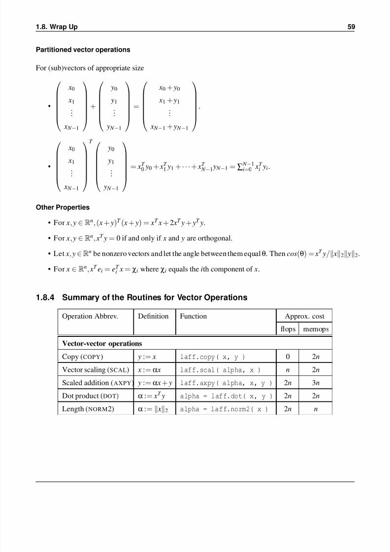
Operation Abbrev. Definition Function Approx. cost
flops memops
Vector-vector operations
Copy (COPY) y := x laff.copy( x, y ) 0 2n
Vector scaling (SCAL) x := α x laff.scal( alpha, x ) n 2n
Scaled addition (AXPY) y := α x
+ y laff.axpy( alpha, x, y ) 2n 3n
Dot product (DOT) α := xT y alpha = laff.dot( x, y ) 2n 2n
Length (NORM2) α := x2 alpha = laff.norm2( x ) 2n n

7/18/2019 Week1
http://slidepdf.com/reader/full/week1-56d46b8915d3b 53/53
Week 1. Vectors in Linear Algebra 566


