Wei_paper for Petrophysic

8/13/2019 Wei_paper for Petrophysic

http://slidepdf.com/reader/full/weipaper-for-petrophysic 1/13

SPWLA 48th

Annual Logging Symposium, June 3-6, 2007

1

INTERPRETATION OF FREQUENCY-DEPENDENT DUAL-

LATEROLOG MEASUREMENTS ACQUIRED IN MIDDLE-EAST

CARBONATE RESERVOIRS USING A SECOND-ORDER FINITE-

ELEMENT METHOD

Wei Yang, and Carlos Torres-Verdín, The University of Texas at Austin; Ridvan Akkurt, Saleh Al-Dossari, and

Abdullah Al-Towijri, Saudi Aramco; Haluk Ersoz, Halliburton

Copyright 2007, held jointly by the Society of Petrophysicists and Well LogAnalysts (SPWLA) and the submitting authors.

This paper was prepared for presentation at the SPWLA 48th Annual LoggingSymposium held in Austin, Texas, United States, June 3-6, 2007.

ABSTRACT

Laterolog tools operate at low frequencies because of

prevalent contact-impedance noise at electrodelocations. However, most existing laterolog modeling

codes are based on zero-frequency (DC) electrical-

potential formulations. In this paper, we develop a newsecond-order finite-element algorithm to simulate the

frequency-dependent laterolog response of axially-

symmetric, invaded and anisotropic formations. Whencompared to first-order (linear) DC finite-element

solutions, the new algorithm provides enhanced

accuracy due to the implementation of second-order

shape functions. In addition, numerical results indicate

that the new algorithm can accurately simulate cases ofextreme contrast in electrical resistivity such as those

arising in the presence of steel casing, air, or anhydrite

layers.

To benchmark the reliability, accuracy, and

applicability of the new simulation algorithm, we

consider the specific electrode configuration ofHalliburton Energy Services’ Dual Laterolog Logging

Tool (DLLT-BTM) to reproduce measurements acquired

in Middle-East carbonate reservoirs. Numerical

simulations incorporate the tool electrode and insulator

dimensions as well as the operating modes of the deep-(LLD) and shallow-sensing (LLS) measurements at

their respective frequencies. Our simulations indicate

that non-DC measurements are affected by the presence

of steel casing. We quantify the influence of anhydritelayers of varying thickness located immediately below

the casing shoe on measurements acquired across porous and permeable carbonate reservoirs. Simulations

show that laterolog apparent resistivities acquired

across low-resistivity carbonate reservoirs shouldered

by anhydrite beds could exhibit a slight bias and also

give a false indication of invasion. In such complex

environments, reliable assessment of hydrocarbonsaturation can only be accomplished with accurate

simulations of laterolog measurements.

INTRODUCTION

Laterolog measurements use a galvanic conduction

principle to excite electrical conduction in rock

formations penetrated by a borehole. While essentiallyDC in nature (Lacour-Gayet, 1981), a strictly zero-

frequency laterolog measurement is impractical due to

contact-impedance noise at electrode locations.

Laterolog measurements are commonly acquired in thefrequency range from 10 Hz to 2 KHz (Anderson,

2001). The application of non-zero values of frequencyoften complicates the interpretation of laterolog

measurements in the presence of large contrasts of

electrical resistivity, including the conspicuous

examples of the so-called Delaware and Groningen

effects (Anderson, 2001, Lacour-Gayet, 1981, Lovell,1993, Trouiller et al., 1978, Woodehouse, 1978).

Most of the available laterolog modeling codes are

based on voltage potential formulations (Li et al., 1995,Yang et al., 1997, Zhang, 1986). Such simulation

methods are strictly accurate only at DC (Lovell, 1993).Lovell (1993) and Zhang (1986) proposed a simulationmethod based on the solution of the partial differential

equation of the current potential. The latter method can

simulate finite-frequency measurements and enables the

efficient calculation of electric current lines. Chen et al.

(1998) utilized the same method for the case of DCsimulations and described the corresponding spatial

distribution of electric current lines. Lovell (1993)

applied a similar simulation method for the non-zerofrequency (AC) case but did not document simulation

results for the case of dual laterolog measurements.

The linear (i.e., first order) finite-element method(FEM) is typically used to simulate laterolog

measurements (Li et al., 1995, Lovell, 1993, Yang et

al., 1997, Zhang, 1986). Experience shows that the

accuracy of the first-order FEM is acceptable in the presence of low to moderate contrasts of electrical

resistivity. However, in extreme contrast situations,

such as those that involve steel casing (resistivity

approximately equal to 2e-7 Ω-m), air, halite, andanhydrite layers (all of them exhibiting practically

infinite electrical resistivity) the accuracy of the first-



SPWLA 48th


2

order FEM is not adequate to reproduce the

measurements.

In this paper, we develop a second-order FEM method

based on the solution of the current potential to

simulate frequency-dependent dual laterologmeasurements in invaded and anisotropic formations.First, we introduce the mathematical formulation, the

associated boundary conditions, and the second-order

FEM variational formulation. We consider the specific

electrode configuration of Halliburton Energy Services’Dual Laterolog Logging Tool (DLLT-BTM) to perform

the numerical simulations. Subsequently, we discussseveral benchmarking examples and draw conclusions

about the accuracy and reliability of our simulation

method. Additional simulation results are discussed

based on laterolog measurements acquired in Middle-

East carbonate formations that include hydrocarbon-

bearing carbonate formations invaded with water-basemud and shouldered by anhydrite beds. The objective

of the latter studies is to assess whether shallow- and

deep-sensing laterolog measurements across porous and permeable carbonate layers remain affected by the

concomitant presence of casing and anhydrite beds.

FORMULATION

Assuming a time harmonic excitation of the form i t e

ω − ,

Maxwell’s equations are given by (Lovell, 1993)

iωμ ∇ × =E H , σ ∇ × = +H E J , (1)

where E and H are the electric and magnetic field

vectors, respectively, μ is the magnetic permeability,

σ is the complex-valued anisotropic conductivity

tensor, J is the impressed current density, σ E is the

induced current density, 1−=i , ω is radian frequency,

and t is time. For the case of transverse-magnetic (TM)

excitation in cylindrical coordinates ( ρ ,φ, z), the onlynon-zero components of the electric and magnetic fields

are , H E φ ρ and

z E . Thus, from Eq. (1) it follows that (Jin

et al., 1999)

1

ˆ ˆ( ) H i H M φ φ φ φ σ φ ωμ −

⋅∇× ∇× + = , (2)

where φ is the unit vector in the azimuthal direction,

and M φ

is the magnetic current density in the

azimuthal direction, defined as

1ˆ ( ) z

z

J J M

z

ρ

φ

ρ

φ σ σ ρ σ

− ⎛ ⎞⎛ ⎞∂ ∂

= ⋅∇× ⋅ = − ⎜ ⎟⎜ ⎟ ⎜ ⎟∂ ∂⎝ ⎠ ⎝ ⎠J , (3)

where ρ σ and

zσ are the horizontal and vertical

electrical conductivities, respectively. Equation (2) can

be written as

( )1 1

z

H H i H M

z z

φ φ

φ φ

ρ

ρ ωμ

ρ ρσ ρ σ

⎛ ⎞∂ ∂⎛ ⎞∂ ∂− − + =⎜ ⎟⎜ ⎟ ⎜ ⎟∂ ∂ ∂ ∂

⎝ ⎠ ⎝ ⎠

. (4)

With the definition 2 J H φ πρ = , we rewrite Eq. (4) as

1 12

z

J J i J M

z z φ

ρ

ωμ π

ρ ρσ ρ ρσ ρ

⎛ ⎞⎛ ⎞∂ ∂ ∂ ∂− − + =⎜ ⎟⎜ ⎟ ⎜ ⎟∂ ∂ ∂ ∂⎝ ⎠ ⎝ ⎠

. (5)

Physically, the connecting lines of J are exactly the

electric current lines excited in the formation by theimpressed galvanic source. In fact, the excitation term

2 M φ π can be imposed with the boundary conditions

shown in Figure 1. Finally, the energy functional used

in our finite-element (FE) simulation algorithm is given by

2 2

21 1 1 1( )

2 z

J J F J i J d dz

z ρ

ωμ ρ π σ ρ σ ρ Ω

⎡ ⎤⎛ ⎞∂ ∂⎛ ⎞= + +⎢ ⎥⎜ ⎟⎜ ⎟∂ ∂⎝ ⎠⎝ ⎠⎢ ⎥⎣ ⎦

∫, (6)

where Ω is the spatial domain of the simulations.

BOUNDARY CONDITIONS AND TOOL

DESCRIPTION

Figure 1 describes the computational domainsΩLLD and

ΩLLS for the deep-and shallow-sensing laterolog modes,

respectively. The domain termination boundary isdenoted as m1. Figure 2 shows the configuration of the

laterolog tool adopted in this paper for the deep- and

shallow-sensing modes. Such a configurationcorresponds to Halliburton Energy Services’ Dual

Laterolog Logging Tool (DLLT-BTM), which operates

at 131.25 Hz for the deep-sensing mode and at 1050 Hzfor the shallow-sensing mode. In Figure 1, the letter B

identifies the current return electrode, placed 33 m

away from the A2 electrode. Electrodes are denoted as

, 1,...,11im i = starting from the electrode placed at

infinity and proceeding counterclockwise. The insulator

adjacent to the electrode im is denoted as im ′ . In the

voltage potential method, homogeneous Neumann

boundary conditions are enforced on insulators (these

conditions are automatically satisfied in finite-elementformulations). We enforce Dirichlet and equipotential

surface boundary conductions at electrode locations,

with the number of boundary conditions equal to the

number of electrodes. Because of the duality of thevoltage potential method, the current potential method

requires the enforcement of boundary conditions on the

insulators, with the number of enforced boundaryconditions equal to the number of insulators. These



SPWLA 48th


3

boundary conditions are given by (Chen et al., 1998):

' '1 1

' '2 2

' ' '3 3 10

' ' ' ' ' ' '4 9 11 4 9 10 11

' '5 5

' '6 6

' ' ' '7 6 7 6

' '8 8

' '9 11

Deep Laterolog Shallow Laterolog

1. 0 0

2. ? ?

3. 0

4. 1 1

5. 0 0

6. ? ?

7.

8. 0 0

9. 1

m m

m m

m m m

m m m m m m m

m m

m m

m m m m

m m

m m

J J

V V

V V V

V V V V V V V

V V

V V

V V V V

V V

V V

= =

= =

= = −

= − = − + = − = − + +

= =

= =

= − = −

= =

= − ' ' '9 10 11

' '10 10

' '11 11

1

10. 0 ?

11. ? ?

m m m

m m

m m

V V V

V V

V V

= − −

= =

= =

(7)

where '

im

V is the voltage decay on insulator'

im . The

above conditions are often referred to as equipotential

surface conditions which have to be enforced by aseries of superposition operations on the finite-element

stiffness matrix (Li et al., 1995, Zhang, 1986).

Conditions on the current potential are of the Dirichlettype and can be enforced directly. In Condition 1, the

current potential J at the top insulator'

1m is defined as

zero. Condition 2 designates '2m

V as an unknown

parameter which needs to be determined by theenforcement of constraint conditions. Condition 3

ensues because the electrode 2 A is always connected

to 2 A ′ . There is an unknown parameter in this equation

for the case of the shallow-sensing mode. However, for

the case of the deep-sensing mode, the voltage

difference between 2 A and 1 A is 0. Condition 4 ensues

because the electrode 1 A is always connected to 1 A′ . In

Condition 5, the voltage difference between the

electrodes 2 M and 1 M is 0. Condition 6 defines '6m

V

as an unknown parameter. Condition 7 ensues because

the electrode 1 M is always connected to 1 M ′ .

Condition 8 enforces that the voltage difference

between 1 M ′

and 2 M ′

be 0. Condition 9 is based onthe fact that the voltage difference between 2 M ′ and

infinity is 1; i.e., ' ' '9 10 11

1m m m

V V V + + = . Condition 10

identifies '10m

V as the zero voltage difference between

electrodes 1 A′ and 2 A ′ (deep-sensing mode) or else as

an unknown parameter (shallow-sensing mode).

Condition 11 designates '11m

V as the unknown voltage

difference between 2 A ′ and infinity.

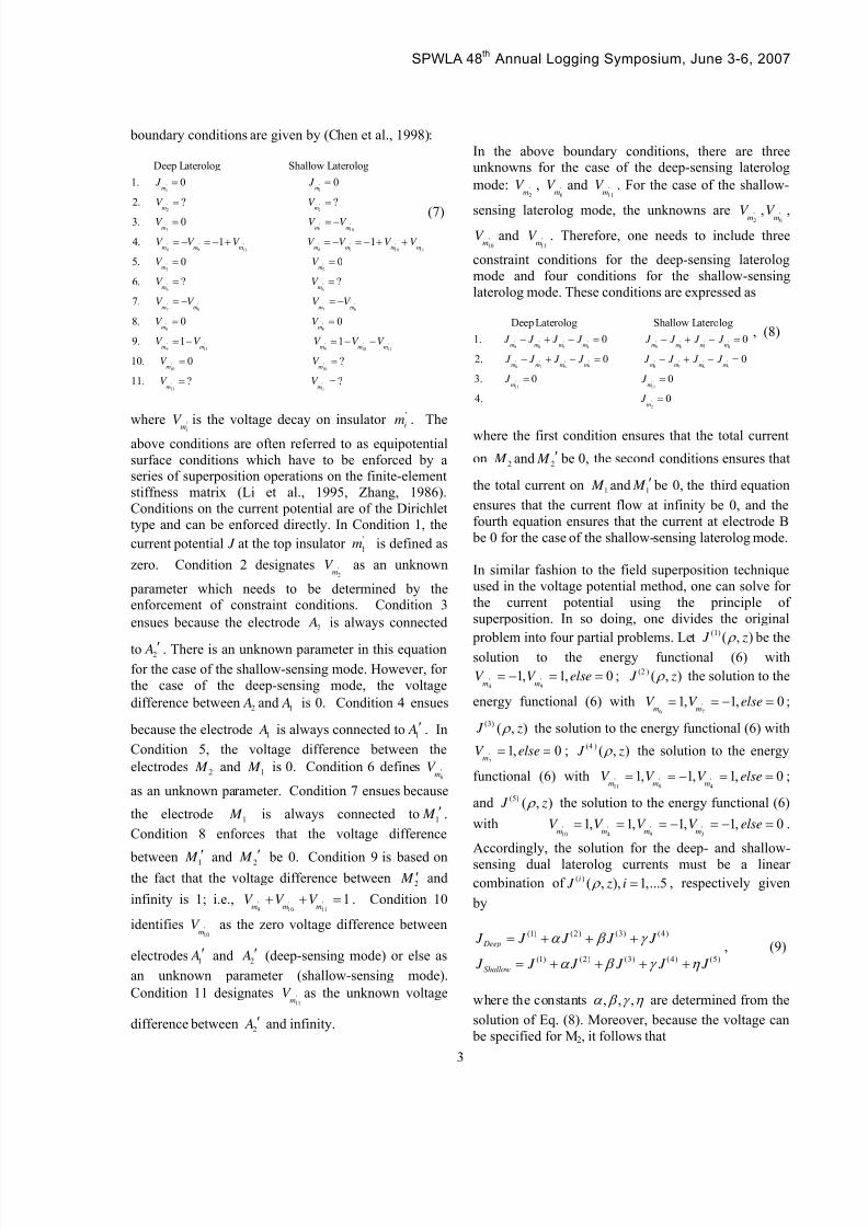
In the above boundary conditions, there are threeunknowns for the case of the deep-sensing laterolog

mode: '2m

V , '6m

V and '11m

V . For the case of the shallow-

sensing laterolog mode, the unknowns are '2mV , '

6mV ,

'10m

V and '11m

V . Therefore, one needs to include three

constraint conditions for the deep-sensing laterolog

mode and four conditions for the shallow-sensing

laterolog mode. These conditions are expressed as

' ' ' ' ' ' ' '9 8 5 4 9 8 5 4

' ' ' ' ' ' ' '8 7 6 5 8 7 6 5

' '11 11

'2

DeepLaterolog Shallow Laterolog

1. 0 0

2. 0 0

3. 0 0

4. 0

m m m m m m m m

m m m m m m m m

m m

m

J J J J J J J J

J J J J J J J J

J J

J

− + − = − + − =

− + − = − + − =

= =

=

, (8)

where the first condition ensures that the total current

on 2 M and 2 M ′ be 0, the second conditions ensures that

the total current on 1 M and 1 M ′ be 0, the third equation

ensures that the current flow at infinity be 0, and the

fourth equation ensures that the current at electrode B

be 0 for the case of the shallow-sensing laterolog mode.

In similar fashion to the field superposition technique

used in the voltage potential method, one can solve for

the current potential using the principle of

superposition. In so doing, one divides the original

problem into four partial problems. Let(1) ( , ) J z ρ be the

solution to the energy functional (6) with

' '4 9

1, 1, 0m m

V V else= − = = ; (2 ) ( , ) J z ρ the solution to the

energy functional (6) with ' '6 7

1, 1, 0m m

V V else= = − = ;

(3)( , ) J z ρ the solution to the energy functional (6) with

'2

1, 0m

V else= = ;(4 )

( , ) J z ρ the solution to the energy

functional (6) with ' ' '11 9 4

1, 1, 1, 0m m m

V V V else= = − = = ;

and (5)( , ) J z ρ the solution to the energy functional (6)

with ' ' ' '10 4 9 3

1, 1, 1, 1, 0m m m m

V V V V else= = = − = − = .

Accordingly, the solution for the deep- and shallow-

sensing dual laterolog currents must be a linear

combination of ( )( , ), 1,...5

i J z i ρ = , respectively given

by

(1) (2) (3) (4)

(1) (2) (3) (4) (5)

Deep

Shallow

J J J J J

J J J J J J

α β γ

α β γ η

= + + +

= + + + +, (9)

where the constants , , ,α β γ η are determined from the

solution of Eq. (8). Moreover, because the voltage can

be specified for M2, it follows that



SPWLA 48th


4

' ' '9 10 11

1m m m

V V V + + = . (10)

The corresponding apparent resistivities are given by

( ) ( )( ) ( ) ( ) ( )

' ' ' '7 6 7 6

1 1,

R R R R Deep deep Shallow shallow

m m m mdeep shallow

R k R k J J J J

= =− −

, (11)

where ,deep shallowk k are the tool constants for deep- and

shallow-sensing laterolog modes, respectively, at 0 Hz.

These constants can be determined from simulations in

a homogenous medium where the measured apparent

resistivities , Deep Shallow R R are equal to the actual

resistivity of the probed medium. The

variables( ) ( )

' '7 6

, R R

m m J J identify the real part of the current

flowing on '7m and '

6m , respectively. Therefore,( ) ( )

' '7 6

R R

m m J J − identifies the real part of the current at the

electrode A0. A similar approach can be used to

calculate out-of-phase apparent resistivities.

SECOND-ORDER FE SOLUTION

To simulate the response of dual laterolog

measurements in the presence of large contrasts ofelectrical conductivity, we make use of second-order

shape functions in the finite-element formulation. The

shape function, shown schematically in Figure 3, is an

8-node quadrilateral element, with the correspondingtwo-dimensional interpolation function given by

2 2 2 2

1 2 3 4 5 6 7 8u x y xy x x x y xyα α α α α α α α = + + + + + + + , (12)

where x and y are the free variables and the subscripted

α values designate arbitrary real-valued constants.

Nodal values of shape function are then given by

[ ] [ ] [ ] [ ]

2

2

T T

1/ 4(1 )(1 )( 1) 1, 2,3, 4

1/ 2(1 )(1 ) 5,7

1/ 2(1 )(1 ) 6,8

1,1,1, 1,0,1,0, 1 , 1, 1,1,1, 1,0,1,0

i i i i i

i i

i i

i i

N i

N i

N i

ξ ξ η η ξ ξ ηη

ξ η η

η ξ ξ

ξ η

= + + + − =

= − + =

= − + =

= − − − = − − −

(13)

Figure 4 compares simulation results obtained with

first- and second-order finite-element methods for thecase of a single-layer invaded isotropic formation.

Figure 5 shows the second model used to compare the

two solution methods. It consists of a single-interface

formation and includes the presence of a borehole andvertically truncated steel casing. Electrical resistivity

contrasts considered in this model are extremely large.

Simulation results, shown in Figure 6, indicate that the

two solutions agree very well in the presence of low to

moderate contrasts of electrical resistivity. However,significant differences between the two methods are

observed in the presence of steel casing. The following

section describes benchmarking exercises undertaken to

appraise the accuracy of the second-order FEMdeveloped in this paper. We also describe examples

intended to study the sensitivity of the simulated

laterolog apparent resistivities to several extreme

conditions of measurement acquisition.

NUMERICAL RESULTS

Code Validation. We first verified the accuracy and

reliability of the new second-order simulation method

against (a) analytical solutions of point sources in a

homogeneous whole space (Zhang, 1986), (b) DCnumerical mode-matching solutions (Liu et al., 1994) in

layered and invaded formations including a borehole,and (c) existing DC first-order laterolog algorithms

based on the solution of the electric potential (Li et al.,

1995, Zhang, 1986) for layered and invaded formationsthat included a borehole. All the simulations were

performed on a Dell Dimension 8400 personal

computer. For the sake of conciseness, we omitgraphical results obtained from the above comparisons.

We note, however, that all the comparisons

conclusively indicated that the accuracy of the new

second-order finite-element algorithm was better than1% even in cases of large contrasts of electrical

resistivity. In what follows, we focus our attention to

specific comparisons performed between first- and

second-order finite-element solutions. All thesimulations are performed specifically for the laterolog

configuration described in Figure 2.

Figure 4 shows results from the first comparison

example at DC. The formation model consists of three

layers with a borehole. Mud resistivity is 1 Ω-m and

borehole diameter is 0.2m One of the layers is invaded.

Layer resistivities are 1, 50, and 1 Ω-m, with theresistivity of the invasion zone in the invaded layer

equal to 10 Ω-m (thickness equal to 2 m and radial

length of invasion equal to 0.2 m). Solid blue (solid

triangles) and dashed blue (open triangles) lines

identify deep laterolog measurements simulated withthe first- and second-order finite-element methods,

respectively. Solid red (solid circles) and dashed red(open circles) lines identify shallow laterolog

measurements simulated with the first- and second-

order finite-element methods, respectively. The dotted

purple line describes the actual value of modelresistivity, Rt . We observe that the two sets of

simulations agree very well with each other.



SPWLA 48th


5

Figure 5 shows the model constructed to perform the

second set of numerical comparisons. It consists of asingle layer interface and includes both a borehole and

steel casing. Mud resistivity is 1 Ω-m and borehole

diameter is 0.2 m. Layer resistivities are 1 and 10000

Ω-m, with their interface located at the relative verticallocation of -1 m. Casing thickness, electrical

resistivity, and relative magnetic permeability are equal

to 0.01 m, 2e-7 Ω-m, and 1, respectively. The lower

termination boundary of casing is located at the relative

vertical location of 1 m and the spatial domain of thesimulation is terminated at the relative vertical location

of 1000 m. Figure 6 describes the simulation resultsobtained with the first- and second-order finite-element

algorithms at DC. Simulations agree very well with

each other along depth segments with low contrasts of

electrical resistivity. However, we note a significantdifference between the two simulation results along the

depth range occupied by steel casing. Further testingwith a numerical mode-matching code indicated that

the relative error of the second-order finite-element

solution was below 1%, thereby confirming thereliability of the new simulation algorithm.

Effect of Electrical Anisotropy. The objective of thissimulation exercise is to shed light to the influence of

resistivity anisotropy on the electrical current lines

enforced within the formation probed by the deep- and

shallow-sensing laterolog modes. We consider aformation with horizontal and vertical resistivities equal

to 1 Ω-m and 2 Ω-m, respectively. Figures 7 and 8

show the electric current lines within the probed

formation calculated for the deep- and shallow-sensinglaterolog modes, respectively. Thick solid lines and thin

dashed lines identify electric current lines for the cases

of isotropic and anisotropic homogeneous formations,respectively. Electric current lines for the anisotropic

formation have a slightly enhanced tendency to flow in

the horizontal direction compared to those of the

isotropic formation because the assumed vertical

resistivity is larger than the vertical resistivity. Inaddition, Figure 8 indicates that electric current lines

for the shallow-sensing laterolog mode are slightly

more sensitive to the presence of electrical anisotropy

than those of the deep-sensing laterolog mode.

Figure 9 compares simulated laterolog measurements

for the cases of isotropic and anisotropic layeredformations. The formation model consists of three

layers (thickness of the center layer is 2 m) and includes

a borehole. Mud resistivity is 1 Ω-m and borehole

diameter is 0.2 m. For the isotropic case, layerresistivities are 1, 10, and 1 Ω-m, whereas for the

anisotropic case, vertical resistivities in the three layers

are 10, 100, and 10 Ω-m, respectively. Solid blue (solid

triangles) and red (solid circles) lines identify deep and

shallow laterolog measurements, respectively,

simulated for the isotropic case. Dashed blue (opentriangles) and red (open circles) lines identify deep- and

shallow-sensing laterolog measurements, respectively,

simulated for the anisotropic case. The dotted purple

and dashed cyan lines identify the actual horizontal ( Rh)and vertical formation resistivities ( Rv), respectively.

Simulations confirm that neither the shallow-sensing

nor the deep-sensing laterolog measurements possess

significant sensitivity to the presence of electrical

anisotropy (this results is consistent with the so-calledanisotropy paradox of laterolog measurements).

However, we observe that shallow-sensing laterologmeasurements exhibit a marginal sensitivity to

electrical anisotropy.

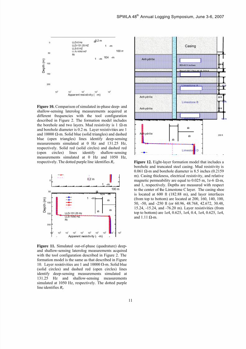
Effect of Non-Zero Probing Frequencies. Figure 10compares simulated in-phase laterolog measurements

for both deep- and shallow-sensing modes at twooperating frequencies. The formation model includes a

borehole and two layers. Mud resistivity is 1 Ω-m and

borehole diameter is 0.2 m. Layer resistivities are 1 and10000 Ω-m. Solid blue (solid triangles) and dashed blue

(open triangles) lines identify deep-sensing

measurements simulated at 0 Hz and 131.25 Hz,respectively. Solid red (solid circles) and dashed red

(open circles) lines identify shallow-sensing

measurements simulated at 0 Hz and 1050 Hz,

respectively. The dotted purple line identifies Rt.Simulations indicate that frequency has no appreciable

effect on laterolog measurements. Figure 11 shows the

simulated out-of-phase (quadrature) laterolog

measurements for both deep- and shallow-sensingmodes at different frequencies. The corresponding

formation model is the same as that shown in Figure 10.

Solid blue (solid circles) and dashed red (open circles)lines identify deep-sensing measurements simulated at

131.25 Hz and shallow-sensing measurements

simulated at 1050 Hz, respectively. The dotted purple

line identifies Rt. Simulations indicate that out-of-phase

laterolog measurements exhibit a similar behavior tothat of the in-phase measurements. However, we note

that the simulated out-of-phase apparent resistivities

require a different normalization constant to that of the

in-phase measurements to properly reproduce the actual

layer resistivities when the resistivity contrast is high.

Multiple Layers in the Presence of Steel Casing. Figure 12 shows an eight-layer model that includes

steel casing. The origin of coordinates is assumed

located at the center of the Limestone C layer, with the

casing shoe located at 600 ft (183 m). Mud resistivity is0.061 Ω-m and borehole diameter is equal to 8.5 inches

(0.2159 m). Casing resistivity, relative magnetic

permeability, and thickness are equal to 1e-6 Ω-m, 1,

and 0.025 m, respectively. Layer interfaces from top to



SPWLA 48th


6

bottom are located at 200, 160, 140, 100, 50, -50, and -

250 ft (or 61, 48.8, 42.7, 30.5, 15.25, -15.25, and -76.25m), respectively. Formation resistivities from top to

bottom are 1e4, 0.625, 1e4, 0.4, 1e4, 0.625, 1e4, and

1.11 Ω-m, respectively. This model was constructed

based on typical Middle East carbonate reservoirs withalternating layers of anhydrite and porous limestone.

The objective of the simulations is to ascertain whether

laterolog apparent resistivities are indicative of actual

resistivities across porous and permeable limestone

layers because of the concomitant presence of anhydritelayers (high electrical resistivity) and steel casing (low

electrical resistivity).

Figures 13 shows the simulated laterolog measurements

at DC for the formation model described in Figure 12.

Figures 14 and 15 show the corresponding simulated in- phase and out-of-phase apparent resistivities,

respectively. Simulations indicate that measurementsacross the various layers are, in general, consistent with

true formation resistivities. However, we note that

apparent resistivities across low-resistivity layers(corresponding to porous and permeable limestone

formations) are slightly different from the

corresponding layer resistivities. The difference between actual layer resistivities and in-phase apparent

resistivities across limestone formations depends on

both frequency and layer thickness. Moreover, we

observe that the simulated deep- and shallow-sensinglaterolog apparent resistivities do not overlap across

low-resistivity limestone layers, thereby opening the

possibility of erroneous interpretations about the

presence and radial extent of mud-filtrate invasion. Asexpected, frequency has a marked effect on the

simulated apparent resistivities across steel casing. The

simulated out-of-phase apparent resistivities aresubstantially different from actual layer resistivities,

possibly due to the fact that the normalizing

geometrical constant should be corrected for frequency.

We also observe anomalous “horns” in the simulated

out-of-phase apparent resistivities across the upperinterfaces of low-resistivity limestone layers.

Figures 16 through 18 show the results of an additional

sensitivity study performed to assess the combined

influence of steel casing and shouldering anhydrite bedson the diagnosis and quantification of invasion. For this

study, invasion was included only in the porous and permeable limestone layers with a single piston-like

invasion front of radial length equal to 1 ft and with

invaded-zone resistivity (Rxo) equal to 0.5 times the

corresponding value of true (uninvaded) formation

resistivity. Comparison of Figures 14 and 16 indicatesthat the effect of casing on the simulated in-phase

apparent resistivities remains only within 100 m of the

casing shoe and does not affect measurements acquired

across porous and permeable limestone layers.

Comparison of Figures 14 through 17 indicates that thesimulated in-phase apparent resistivities remain

sensitive to the presence of invasion regardless of the

presence of both casing and shouldering anhydrite beds.

In particular, the simulated shallow-sensing apparentresistivities exhibit an almost linear sensitivity to the

corresponding perturbation of invaded-zone resistivity

regardless of the presence of both casing and anhydrite

shouldering beds.

CONCLUSIONS

We have formulated, implemented, and successfully

tested a new second-order finite-elemnt method to

simulate axially-symmetric laterolog measurements

based on the variational formulation of the frequency-dependent current potential. Benchmarking exercises

confirmed the reliability and accuracy of the simulationmethod in the presence of large contrasts of electrical

resistivity, electrical anisotropy, and invasion. Specific

simulations conducted for the case of HalliburtonEnergy Services’ Dual Laterolog Logging Tool (DLLT-

BTM) configuration indicate that the placement of the

return current electrode, N, at infinity has a negligibleeffect on non-zero frequency measurements. We found

that steel casing has a significant effect on shallow- and

deep-sensing laterolog measurements. The effect of

steel casing on both in-phase and out-phase laterologmeasurements depends on the specific value of

frequency. Moreover, simulations indicate that the

effect of steel casing remains confined to the spatial

neighborhood of casing (within 100 m) with marginaleffect on apparent resistivities measured tens of feet

away from the casing shoe, even in the extreme case of

presence of highly resistive layers of anhydrite. Oursimulations indicate measurable differences between

true layer resistivities and laterolog apparent

resistivities across porous and permeable limestone

layers shouldered by anhydrite beds. Simulations also

revealed separation between shallow- and deep-sensinglaterolog measurements across porous and permeable

limestone layers shouldered by anhydrite beds that

could give a false indication of invasion. In cases of

significant variations of layer resistivities, the work

presented in this paper suggests that the petrophysicalinterpretation of laterolog apparent resistivities should

be guided by numerical simulation.

ACKNOWLEDGEMENTS

The work reported in this paper was funded byUniversity of Texas at Austin Research Consortium on

Formation Evaluation, jointly sponsored by Anadarko,

Aramco, Baker Atlas, BP, British Gas, ConocoPhilips,

Chevron, ENI E&P, ExxonMobil, Halliburton Energy



SPWLA 48th


7

Services, Hydro, Marathon Oil Corporation, Mexican

Institute for Petroleum, Occidental PetroleumCorporation, Petrobras, Schlumberger, Shell

International E&P, Statoil, TOTAL, and Weatherford.

REFERENCES

Anderson, B. I., 2001, Modeling and inversion methods

for the interpretation of resistivity logging tool

response: PhD Thesis, Delft University of

Technology.Chen Y. H., Chew W. C. and Zhang G. J., 1998, A

novel array laterolog method: The Log Analyst, v.39, no. 5, pp. 23-33.

Jin J. M., M. Zunoubi, K. C. Donepudi, and W. C.

Chew, 1999, Frequency-domain and time-domain

finite-element solution of Maxwell’s equationsusing the spectral Lanczos decomposition method:

Computer Methods in Applied Mechanics andEngineering, v. 169, no. 1999, pp. 279-296.

Lacour-Gayet, P., 1981, The Groningen effect, causes

and a partial remedy: Schlumberger TechnicalReview, v. 29, no. 1, pp. 37-47.

Li, T. T., and Tan, Y.J., 1995, Mathematical problems

and methods in resistivity well-logging: SurveysMath. Industry, v. 5, pp 133-167.

Liu, Q. H., Anderson, B., and Chew, W.C., 1994,

Modeling low-frequency electrode-type resistivity

tools in invaded thin beds: IEEE Transactions onGeoscience and Remote Sensing, v. 32, no. 3.

Lovell, J. R., 1993, Finite element methods in

resistivity logging: PhD Thesis, Delft University of

Technology.Trouiller J. C., and Dubourg I., 1978, A better deep

laterolog compensated for Groningen and reference

effects: in Transactions of the 35th SPLWASymposium, pp. 1-16, Paper VV.

Woodehouse, R., 1978, The laterolog Groningen

phantom can cost you money: in Transactions of

the 19th SPLWA Symposium, pp. 1-17, Paper R.

Yang F., and Nie Z. P., 1997, A precise numericalsimulation of DLL logging response: Chinese Well

Logging Technology, v. 21, no. 4.

Zhang, G. J., 1986, Electrical well logging (II) (in

Chinese): The Petroleum Industry Press, Beijing.

ABOUT THE AUTHORS

Wei Yang received a Ph.D. degree in GeneralMechanics from Harbin Institute of Technology, China,

in 1995. During 1995-1997 he was a postdoctoral

researcher at the University of Petroleum, Beijing,China. During 1997-2005, he held the position of

Associate Professor with the Borehole Research Center

of the same university. From 2005 to 2006, he was a

Research Fellow with the Department of Petroleum and

Geosystems Engineering of The University of Texas at

Austin. Since December 2006, he has been withWesternGeco Electromagnetics of Schlumberger as

Senior Research Scientist. He conducts research on

marine CSEM and MT. He published over 30 papers

and holds a Chinese patent.

Carlos Torres-Verdín received a Ph.D. degree in

Engineering Geoscience from the University ofCalifornia, Berkeley, in 1991. During 1991–1997 he

held the position of Research Scientist with

Schlumberger-Doll Research. From 1997–1999, he wasReservoir Specialist and Technology Champion with

YPF (Buenos Aires, Argentina). Since 1999, he has

been with the Department of Petroleum andGeosystems Engineering of The University of Texas at

Austin, where he currently holds the position of

Associate Professor. He conducts research on borehole

geophysics, well logging, formation evaluation, andintegrated reservoir characterization. Torres-Verdín has

served as Guest Editor for Radio Science, and iscurrently a member of the Editorial Board of the

Journal of Electromagnetic Waves and Applications,

and an associate editor for Petrophysics (SPWLA) and

the SPE Journal. He is co-recipient of the 2003 and2004 Best Paper Award by Petrophysics, and is

recipient of SPWLA’s 2006 Distinguished TechnicalAchievement Award.

Ridvan Akkurt is a Petroleum Engineering Consultant

at Aramco. Ridvan started his oilfield career in 1983 inAfrica as a wireline field engineer for Schlumberger,

then worked for GSI in the Middle East as a fieldseismologist, for Schlumberger-Doll Research on NMR

research, for Shell as a geophysicist, and for NUMAR

as a senior research scientist. He founded NMRPLUS

in late 1997, and consulted for major oil and servicecompanies on various aspects of NMR logging until

joining Aramco in 2005. Ridvan has a B.Sc. degree inElectrical Engineering from the Massachusetts Institute

of Technology and a Ph.D. degree in Geophysics from

the Colorado School of Mines. He has several

publications and patents in the area of NMR logging, isrecipient of best paper award by SPWLA in 1995,

teaches industrial courses on NMR logging, and has

served as a Distinguished Lecturer for SPE during1998-1999, and for SPWLA during 1995-1996.

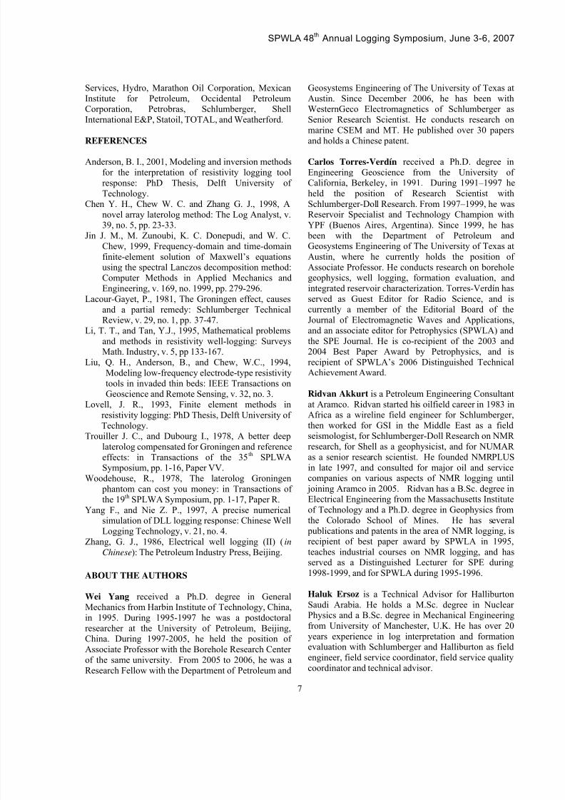
Haluk Ersoz is a Technical Advisor for Halliburton

Saudi Arabia. He holds a M.Sc. degree in NuclearPhysics and a B.Sc. degree in Mechanical Engineering

from University of Manchester, U.K. He has over 20

years experience in log interpretation and formationevaluation with Schlumberger and Halliburton as field

engineer, field service coordinator, field service quality

coordinator and technical advisor.



SPWLA 48th


8

(a)

(b)

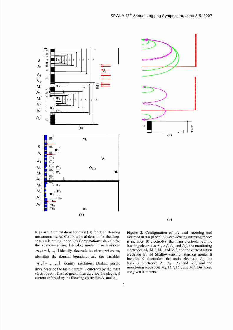
Figure 1. Computational domain (Ω) for dual laterologmeasurements. (a) Computational domain for the deep-

sensing laterolog mode. (b) Computational domain forthe shallow-sensing laterolog model. The variables

, 1,...,11i

m i = identify electrode locations, where m1

identifies the domain boundary, and the variables

, 1,...,11im i′ = identify insulators. Dashed purple

lines describe the main current I0 enforced by the mainelectrode A0 . Dashed green lines describe the electrical

current enforced by the focusing electrodes A1 and A2.

(a)

(b)

Figure 2. Configuration of the dual laterolog toolassumed in this paper. (a) Deep-sensing laterolog mode:

it includes 10 electrodes: the main electrode A0, the

bucking electrodes A1, A1’, A2 and A2’, the monitoringelectrodes M1, M1’, M3, and M3’, and the current return

electrode B. (b) Shallow-sensing laterolog mode: It

includes 9 electrodes: the main electrode A0, the bucking electrodes A1, A1’, A2 and A2’, and the

monitoring electrodes M1, M1’, M2, and M2’. Distances

are given in meters.

m1

B

A2

A1

M3

M1

A0

A1’

A2’

M1’

M3’

m1

m1

m1

’

m2 m2

’

m3

m3

’

m4

m4

’ m5

m5

’

m6

m6

’

m7

m7

’

m8

m8

’

m9

m9

’ m10

m10

’

m11

m11

’

ΩLLD

V0

I0

vvv

m1

B

A2

A1

M2

M1 A0

A1’

A2’

M1’

M2’

m1

m1

m1

’

m2 m2

’

m3

m3

’

m4

m4

’ m5

m5

’

m6 m6’

m7

m7

’

m8

m8

’

m9

m9

’ m10

m10

’

m11

m11

’

ΩLLS

V0

I0



SPWLA 48th


9

Figure 3. Description of the 8-node quadrilateral

element used in the second-order finite-elementformulation.

2

1

0

-1

-2

1 10 100

1 -m

2 m50 -m10 -m0.2m

1 -m

1 -m0.2m

Apparent Resist ivi ty ( -m)

D e p t h ( m )

FIRST ORDER-LLD

SECOND ORDER-LLD

FIRST ORDER-LLS

SECOND ORDER-LLS

Rt

Figure 4. Comparison of first- and second-order finite-

element solutions. Figure 2 shows the assumedlaterolog tool configuration operating at 0 Hz. The

formation model includes three layers with a borehole.Mud resistivity is 1 Ω-m and borehole diameter is 0.2m

One of the layers is invaded. Layer resistivities are 1,

50, and 1 Ω-m, with the resistivity of the invasion zone

in the invaded layer equal to 10 Ω-m (thickness equal to2 m and radial length of invasion equal to 0.2 m). Solid

blue (solid triangles) and dashed blue (open triangles)

lines identify deep laterolog measurements simulated

with the first- and second-order finite-element methods,

respectively. Solid red (solid circles) and dashed red(open circles) lines identify shallow laterolog

measurements simulated with the first- and second-

order finite-element methods, respectively. The dotted purple line identifies Rt .

Figure 5. Single-interface formation model with

borehole and steel casing. Mud resistivity is 1Ω

-m and borehole diameter is 0.2 m. Layer resistivities are 1 and

10000 Ω-m, with their interface located at the relativevertical location of -1 m. Casing thickness, electrical

resistivity, and relative magnetic permeability are equal

to 0.01 m, 2e-7 Ω-m, and 1, respectively. The lower

termination boundary of casing is located at a the

relative vertical location of 1 m and the spatial domainof the simulation is terminated at the relative vertical

location of 1000 m.

-2

-1

0

1

2

10-3

10-2

10-1

100

101

102

103

104

105

Apparent Resist ivit y ( -m)

D e p t h ( m )

FIRST ORDER-LLD

SECOND ORDER-LLD

FIRST ORDER-LLS

SECOND ORDER-LLS Rt

Figure 6. Comparison of first- and second-order finite-element solutions for the formation model described inFigure 5. Figure 2 shows the assumed laterolog tool

configuration operating at 0 Hz. Solid blue (solid

triangles) and dashed blue (open triangles) linesidentify deep laterolog measurements simulated with

the first- and second-order finite-element methods,

respectively. Solid red (solid circles) and dashed red

(open circles) lines identify shallow laterologmeasurements simulated with the first- and second-

order finite-element methods, respectively. The dotted

purple line identifies Rt .



SPWLA 48th


10

0.5 1 1.5 2 2.5 3 3.5 4 4.5 5

-2.5

-2

-1.5

-1

-0.5

0

0.5

1

1.5

2

2.5

Radial Coordinate (m)

V e r t i c a l C o o r d i n a t e (

m )

Figure 7. Spatial distribution of electric current lines

for deep-sensing laterolog measurements simulated

across isotropic and anisotropic homogeneousformations. The horizontal and vertical resistivities of

the formation are 1 Ω-m and 2 Ω-m, respectively. Thick

solid lines and thin dashed lines identify electric current

lines for the cases of isotropic and anisotropichomogeneous formations, respectively.

0.5 1 1.5 2 2.5 3 3.5 4 4.5 5

-2.5

-2

-1.5

-1

-0.5

0

0.5

1

1.5

2

2.5

Radial Coordinate (m)

V e r t i c a l C o o r

d i n a t e ( m )

Figure 8. Spatial distribution of electric current lines

for shallow-sensing laterolog measurements simulatedacross isotropic and anisotropic homogeneous

formations. The horizontal and vertical resistivities of

the formation are 1 Ω-m and 2 Ω-m, respectively. Thicksolid lines and thin dashed lines identify electric current

lines for the cases of isotropic and anisotropic

homogeneous formations, respectively.

2

1

0

-1

-2

1 10

1 -m

0.2m

2m10 -m

1 -m 1 -m

Apparent Resistivity ( -m)

D e p t h ( m )

LLD_Iso

LLS_Iso

Rt

(a)

2

1

0

-1

-2

1 10 100

Rh=10,Rv=100 -m

Rh=1,Rv=10 -m1 -m

0.2m

2m

Rh=1,Rv=10 -m

Apparent Resisti vity ( -m)

D e p t h ( m )

LLD_Ani

LLS_Ani

Rh

Rv

(b)

Figure 9. Simulation of dual laterolog measurements in(a) isotropic and (b) anisotropic inhomogeneous

formations. The formation model consists of three

layers (thickness of center layer is 2 m) and includes a

borehole. Mud resistivity is 1 Ω-m and borehole

diameter is 0.2 m. For the isotropic case, layerresistivities are 1, 10, and 1 Ω-m, whereas for the

anisotropic case, vertical resistivities in the three layers

are 10, 100, and 10 Ω-m, respectively. Figure 2 showsthe assumed tool configuration; the operating frequency

is 0 Hz. Solid blue (solid triangles) and red (solid

circles) lines identify deep and shallow laterologmeasurements, respectively, simulated for the isotropic

case. Dashed blue (open triangles) and red (open

circles) lines identify deep and shallow laterolog

measurements, respectively, simulated for the

anisotropic case. The dotted purple and dashed cyan

lines identify the horizontal ( Rh) and vertical

resistivities ( Rv), respectively.



SPWLA 48th


11

200

150

100

50

0

100

101

102

103

104

Apparent resi stivity ( -m)

0.2 m

1 -m

100 m

1E4 -m

1 -m

D e p t h ( m

)

LLD-0 Hz

LLD-131.25 HZ

LLS-0 HZ

LLS-1050 HZ

Rt

Figure 10. Comparison of simulated in-phase deep- and

shallow-sensing laterolog measurements acquired at

different frequencies with the tool configuration

described in Figure 2. The formation model includesthe borehole and two layers. Mud resistivity is 1 Ω-m

and borehole diameter is 0.2 m. Layer resistivities are 1and 10000 Ω-m. Solid blue (solid triangles) and dashed

blue (open triangles) lines identify deep-sensing

measurements simulated at 0 Hz and 131.25 Hz,respectively. Solid red (solid circles) and dashed red

(open circles) lines identify shallow-sensing

measurements simulated at 0 Hz and 1050 Hz,

respectively. The dotted purple line identifies Rt .

200

150

100

50

0

10-1

100

101

102

103

104

105

106

107

108

Apparent resis tiv ity ( -m)

1 -m

1 -m

0.2 m

100 m

1E4 -m

D e p t h ( m )

LLD-131.25 Hz

LLS-1050 HZ

Rt

Figure 11. Simulated out-of-phase (quadrature) deep-and shallow-sensing laterolog measurements acquired

with the tool configuration described in Figure 2. The

formation model is the same as that described in Figure

10. Layer resistivities are 1 and 10000Ω-m. Solid blue

(solid circles) and dashed red (open circles) linesidentify deep-sensing measurements simulated at

131.25 Hz and shallow-sensing measurements

simulated at 1050 Hz, respectively. The dotted purple

line identifies Rt .

Figure 12. Eight-layer formation model that includes a

borehole and truncated steel casing. Mud resistivity is0.061 Ω-m and borehole diameter is 8.5 inches (0.2159

m). Casing thickness, electrical resistivity, and relative

magnetic permeability are equal to 0.025 m, 1e-6 Ω-m,

and 1, respectively. Depths are measured with respectto the center of the Limestone C layer. The casing shoe

is located at 600 ft (182.88 m), and layer interfaces

(from top to bottom) are located at 200, 160, 140, 100,

50, -50, and -250 ft (or 60.96, 48.768, 42.672, 30.48,15.24, -15.24, and -76.20 m). Layer resistivities (from

top to bottom) are 1e4, 0.625, 1e4, 0.4, 1e4, 0.625, 1e4,

and 1.11 Ω-m.

Limestone A

Anh ydr it e

400 ft

Limestone B

Limestone C

Limestone D

Anh ydr ite

Anh ydr ite

Anh ydr ite

40 ft

20 ft

40 ft

50 ft

100 ft

200 ft

BS=8.5 inches

Rm=0.061 Ohm-M @ 223 F

Casing

Limestone A

Anh ydr it e

400 ft

Limestone B

Limestone C

Limestone D

Anh ydr ite

Anh ydr ite

Anh ydr ite

40 ft

20 ft

40 ft

50 ft

100 ft

200 ft

BS=8.5 inches

Rm=0.061 Ohm-M @ 223 F

Casing



SPWLA 48th


12

-100

-50

0

50

100

150

200

10-1

100

101

102

103

104

Resistivity ( -m)

D e p t h ( m

)

Rt LLD-0 Hz

LLS-0 Hz

Figure 13. Deep- and shallow-sensing laterolog

measurements simulated at DC for the formation modelshown in Figure 12 and with the tool configuration

described in Figure 2. The solid black line identifiesvalues of true (uninvaded) formation resistivity. Solid

blue (solid circles) and dashed red (open circles) lines

identify the simulated deep- and shallow-sensingsensing laterolog measurements, respectively.

-100

-50

0

50

100

150

200

10-1

100

101

102

103

104

Resistivity ( -m)

D e p t h ( m

)

Rt LLD-131.25 Hz

LLS-1050 Hz

Figure 14. In-phase apparent resistivities of deep- and

shallow-sensing laterolog measurements simulated for

the formation model shown in Figure 12 with the toolconfiguration described in Figure 2. The solid black

line identifies values of true (uninvaded) formationresistivity. Solid blue (solid circles) and dashed red

(open circles) lines identify the simulated deep- (131.25

Hz) and shallow-sensing (1050 Hz) laterologmeasurements.

-100

-50

0

50

100

150

200

10-2

10-1

100

101

102

103

104

105

106

107

108

Resistivi ty ( -m)

D e p t h ( m

)

Rt

LLD-131.25 Hz

LLS-1050 Hz

Figure 15. Out-of-phase apparent resistivities of deep-

and shallow-sensing laterolog measurements simulated

for the formation model shown in Figure 12 with thetool configuration described in Figure 2. The solid

black line identifies values of true (uninvaded)

formation resistivity. Solid blue (solid circles) anddashed red (open circles) lines identify the simulated

deep- (131.25 Hz) and shallow-sensing (1050 Hz)

laterolog measurements.

-100

-50

0

50

100

150

200

10-1

100

101

102

103

104

Resistivi ty ( -m)

D e p t h ( m

)

Rt LLD-131.25 Hz

LLS-1050 Hz



the formation model shown in Figure 12 with the tool

configuration described in Figure 2. Casing was notincluded in the simulations. The solid black line

identifies values of true (uninvaded) formation

resistivity. Solid blue (solid circles) and dashed red(open circles) lines identify the simulated deep- (131.25

Hz) and shallow-sensing (1050 Hz) laterolog

measurements (cf. Figs. 14, 17, and 18).



SPWLA 48th


13

-100

-50

0

50

100

150

200

10-1

100

101

102

103

104

Resistivity ( -m)

D e p t h ( m

)

Rt

LLD-131.25 Hz

LLS-1050 Hz



the formation model shown in Figure 12 with the toolconfiguration described in Figure 2. Casing was not

included in the simulations whereas invasion was only

included in the low-resistivity limestone beds ( R xo = Rt /2 and radial length of invasion equal to 1 ft). The solid

black line identifies values of true (uninvaded)

formation resistivity. Solid blue (solid circles) and

dashed red (open circles) lines identify the simulated

deep- (131.25 Hz) and shallow-sensing (1050 Hz)laterolog measurements (cf. Figs. 14, 16, and 18).

-100

-50

0

50

100

150

200

10-1

100

101

102

103

104

Resistivity ( -m)

D e p t h ( m

)

Rt

LLD-131.25 Hz

LLS-1050 Hz



the formation model shown in Figure 12 with the toolconfiguration described in Figure 2. Both casing and

invasion were included in the simulations. Invasion was

only included in the low-resistivity limestone beds

( R xo= Rt /2 and radial length of invasion equal to 1 ft).The solid black line identifies values of true

(uninvaded) formation resistivity. Solid blue (solid

circles) and dashed red (open circles) lines identify thesimulated deep- (131.25 Hz) and shallow-sensing (1050

Hz) laterolog measurements (cf. Figs. 14, 16, and 17).

Date post:	04-Jun-2018
Category:	Documents
Upload:	yangwei00414312
View:	221 times
Download:	0 times

Wei_paper for Petrophysic

Documents