Page 1
Welfare-Based Optimal Macroprudential Policy with Shadow
Banks Stefan Gebauer1
June 2021, WP #817
ABSTRACT
In this paper, I show that the existence of non-bank financial institutions (NBFIs) has implications for the optimal regulation of the traditional banking sector. I develop a New Keynesian DSGE model for the euro area featuring a heterogeneous financial sector allowing for potential credit leakage towards unregulated NBFIs. Introducing NBFIs raises the importance of credit stabilization relative to other policy objectives in the welfare-based loss function of the regulator. The resulting optimal policy rule indicates that regulators adjust dynamic capital requirements more strongly in response to macroeconomic shocks due to credit leakage. Furthermore, introducing non-bank finance not only alters the cyclicality of optimal regulation, but also has implications for the optimal steady-state level of capital requirements and loan-to-value ratios. Sector-specific characteristics such as bank market power and risk affect welfare gains from traditional and NBFI credit.2
Keywords: Macroprudential Regulation, Monetary Policy, Optimal Policy, Non-Bank Finance, Shadow Banking, Financial Frictions
JEL classification: E44, E61, G18, G23, G28
1 Banque de France, [email protected] 2 Acknowledgments and disclaimer: I thank Mathias Trabandt for detailed feedback and support. I am also indebted to Flora Budianto, Michael Burda, Marius Clemens, Marcel Fratzscher, Martín Harding, Yannick Kalantzis, Falk Mazelis, Federico di Pace, Karl Walentin, Lutz Weinke and participants at the Econometric Society European Winter Meeting 2019, Rotterdam, the Third Research Conference of the CEPR Macroeconomic Modelling and Model Comparison Network (MMCN), Frankfurt am Main, the 2019 Spring Meeting of Young Economists, Brussels, and research seminars at Banque de France, Bank of England, the European Central Bank, Bundesbank, Bank of Latvia, FU Berlin and Humboldt University Berlin for valuable comments and remarks. Working Papers reflect the opinions of the authors and do not necessarily express the views of the Banque de
France and of the European Central Bank. This document is available on publications.banque-france.fr/en
Page 2
Banque de France WP #817 ii
NON-TECHNICAL SUMMARY
The relevance of non-bank financial institutions (NBFIs) for financial stability has recently been addressed by financial regulators. For instance, imbalances in the non-bank financial sector have been identified as a main risk to financial stability in the euro area during the Covid-19 pandemic. Furthermore, the importance of NBFIs has been acknowledged in recent discussions on a “Capital Markets Union (CMU)” in Europe. However, designing a macroprudential framework for the non-bank financial sector similar to the approach applied to commercial banks is barely feasible. While traditional banks directly intermediate funds between borrowers and savers, a multitude of specialized financial corporations operating in complex intermediation chains are usually involved in non-bank credit intermediation.
Nevertheless, changes in macroprudential regulation for the commercial banking sector can shift credit intermediation towards less regulated parts of the financial system. For instance, higher capital requirements for traditional banks potentially lead to credit leakage towards unregulated NBFIs: As tighter banking regulation does not initially affect credit demand, higher regulation for commercial banks may incentivize borrowers to switch to NBFIs as commercial bank credit becomes relatively costly. Consequently, prudential authorities need to decide on an optimal level of regulation such that on the one side, banks' equity buffers are sufficiently high, but on the other side credit leakage to non-banks is limited.
In this paper, I study the optimal design of bank capital requirements and loan-to-value (LTV) ratios in the presence of a non-bank financial sector. I base the analysis on a New-Keynesian dynamic stochastic general equilibrium (DSGE) model featuring a heterogeneous financial sector calibrated to match economic and financial conditions in the euro area. The findings on optimal policy reveal that in the presence of NBFIs, the welfare-optimal level of static capital requirements is lower (13.5 percent) than in a counterfactual scenario where credit is intermediated only by traditional banks (16 percent). I highlight that the difference in optimal regulation can be attributed to an additional trade-off the regulator has to take into account, which relates to the composition of credit provided by commercial banks and NBFIs. Furthermore, NBFI presence affects the optimal dynamic response of macroprudential regulation to fluctuations in output and credit. Whenever macroeconomic disturbances imply credit leakage towards NBFIs, regulatory adjustments are more pronounced as in an economy without non-bank finance.
I then show that the additional policy trade-off is shaped by structural characteristics of financial institutions. For instance, empirical evidence suggests a significant degree of market power in the euro area commercial banking sector. In contrast, some studies find that non-bank finance can increase efficiency in financial markets by providing alternative financing sources and due to the involvement of highly specialized institutions in the intermediation process. However, NBFI intermediation can increase systemic risk, as structural characteristics, economic motivations, and regulatory constraints within the diverse non-bank financial sector can accelerate financial stress and macroeconomic disturbances, and finally pose a threat to financial stability.
In summary, the findings indicate that neglecting NBFIs potentially impairs the efficiency of macroprudential policies, as regulators do not internalize credit leakage and an additional trade-off related to the composition of credit. Thus, they should consider developments in the non-bank financial sector, even if their policies only apply to traditional banks. Furthermore, the lack of macroprudential tools for NBFIs raises potential gains from coordinating the implementation of different macroprudential policy measures. In addition, coordination with monetary policy can play a role, as NBFIs' activity is also related to the overall price of credit in the economy. Thus, credit leakage may be aggravated when the effective lower bound (ELB) on nominal interest rates is reached.
Page 3
Banque de France WP #817 iii
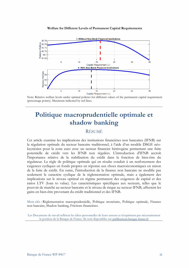
Welfare for Different Levels of Permanent Capital Requirements
Note: Relative welfare levels under optimal policies for different values of the permanent capital requirement (percentage points). Maximum indicated by red lines.
Politique macroprudentielle optimale et shadow banking
RÉSUMÉ
Cet article examine les implications des institutions financières non bancaires (IFNB) sur la régulation optimale du secteur bancaire traditionnel, à l’aide d’un modèle DSGE néo-keynésien pour la zone euro avec un secteur financier hétérogène permettant une fuite potentielle de crédit vers les IFNB non régulées. L'introduction d'IFNB accroît l'importance relative de la stabilisation du crédit dans la fonction de bien-être du régulateur. La règle de politique optimale qui en résulte conduit à un renforcement des exigences cycliques en fonds propres en réponse aux chocs macroéconomiques en raison de la fuite de crédit. En outre, l'introduction de la finance non bancaire ne modifie pas seulement le caractère cyclique de la réglementation optimale, mais a également des implications sur le niveau optimal en régime permanent des exigences de capital et des ratios LTV (loan to value). Les caractéristiques spécifiques aux secteurs, telles que le pouvoir de marché au secteur bancaire et le niveau de risque au secteur IFNB, affectent les gains en bien-être provenant du crédit traditionnel et des IFNB.
Mots-clés : Réglementation macroprudentielle, Politique monétaire, Politique optimale, Finance non bancaire, Shadow banking, Frictions financières.
Les Documents de travail reflètent les idées personnelles de leurs auteurs et n'expriment pas nécessairement la position de la Banque de France. Ils sont disponibles sur publications.banque-france.fr
Page 4
1 Introduction
The financial crisis of 2007/2008 triggered a substantial debate about the optimal
stance of financial regulation. As of today, a broad consensus on the necessity of a
macroprudential approach to target systemic developments in financial markets has
been reached among scholars and policy makers.1 Contemporaneously, the neglected
treatment or complete absence of financial intermediaries and frictions in canonical
pre-crisis dynamic stochastic general equilibrium (DSGE) models has widely been
criticized. In response, banking-augmented macro models have been developed and
employed to assess, inter alia, the effectiveness of different macroprudential tools in
the presence of financial frictions. In particular, significant progress has been made
with respect to the consideration of commercial banking at the macro level, both in
theoretical models and in the field of financial regulation.
In comparison, the role of non-bank financial intermediation2 has for a long time
been understated in both areas. Only recently, the introduction of heterogeneous
financial sectors in macro models has been initiated. On the policy side, the im-
portance of non-banks has been acknowledged in the recent and ongoing debate on
the optimal design of a “Capital Markets Union (CMU)” in Europe.3 Also, imbal-
ances in the non-bank financial sector have been identified as main risks for financial
stability in the euro area during the current Covid-19 pandemic.4
The shift in attention towards NBFIs finally reflects the fact that non-bank fi-
nance has substantially gained importance in the euro area over the last two decades.
Figure 1 shows the evolution of the total amount of outstanding credit to non-
financial corporations, provided by traditional banks and non-bank financial inter-
mediaries in the euro area.5 Whereas commercial banks provide the largest share
1See Borio (2011, 2009) or Borio and Shim (2007) for a detailed description of the macropru-
dential approach. For a review of the pre-crisis microprudential approach, see Kroszner (2010),
Borio (2003), or Allen and Gale (2000).
2In this paper, the terms “non-bank financial intermediation” and “shadow banking” will be
used interchangeably to describe credit intermediation outside the regulated traditional commercial
banking sector. See for instance Adrian and Jones (2018) for a discussion on terminology.
3In a CMU, non-bank finance could play an important role to mitigate bank-dependency in the
European financial sector, but would require further strengthening of regulatory measures. See for
instance Pires (2019).
4See for instance ECB Financial Stability Review, May 2021.
5Non-bank credit is defined as the aggregate loans provided by “Other Financial Intermedi-
aries”, a composite of different financial corporations other than commercial banks or institutions
2
Page 5
of lending to corporates, non-bank lending has steadily increased since the imple-
mentation of the euro and has currently reached more than 35 percent of traditional
lending.
Figure 1: Commercial and Non-Bank Loans to Non-Financial Corporates
0
5
10
15
20
25
30
35
40
0
1000
2000
3000
4000
5000
6000
1999 2001 2003 2005 2007 2009 2011 2013 2015 2017 2019
Pe
rcen
t
Bn
. E
UR
OFI sector Commercial bank sector OFI/Commercial bank (rhs)
Note: Outstanding amount of loans of commercial banks and non-banks (OFI) to non-financial
corporates (billions of euro). Source: Euro Area Accounts and Monetary Statistics (ECB).
In this paper, I discuss optimal macroprudential policies while allowing credit
to be intermediated by both commercial and non-bank financial intermediaries
(NBFIs). I base the analysis on a New Keynesian DSGE model featuring a hetero-
geneous financial sector similar to the one derived in Gebauer and Mazelis (2020).
NBFIs and commercial banks differ in the degree of competitiveness and risk and
are affected to a different degree by regulation. Methodologically, the framework
combines elements of two leading strands of the literature on financial frictions in
DSGE models that appear well-suited to model these structural and regulatory dif-
ferences. For the commercial banking sector, a financial framework similar to the
belonging to the Eurosystem. However, alternative measures of non-bank credit can straightfor-
wardly be derived by marginal adjustments of OFI aggregates. See for instance Gebauer and
Mazelis (2020), Doyle et al. (2016) or Bakk-Simon et al. (2012).
3
Page 6
one derived in Gerali et al. (2010) is introduced which allows explicitly for com-
mercial bank capital regulation. Furthermore, it features structural elements that
describe the banking sector in the euro area well. For NBFIs, elements of the bank-
ing framework developed in Gertler and Karadi (2011) are introduced. Instead of
being affected by banking regulation, non-bank credit is limited by a moral haz-
ard friction between investors and NBFIs that results in an endogenous leverage
constraint.
To discuss optimal regulation, I derive welfare loss functions and optimal policies
under commitment following a “linear-quadratic (LQ)” approach as introduced in
the literature on monetary policy. The approach relies in large part on the deriva-
tion of optimal policy under the timeless perspective developed in Giannoni and
Woodford (2003a,b), Benigno and Woodford (2005, 2012) and Woodford (2011). I
derive optimal policy under commitment to study the design of an optimal policy
rule to which a macroprudential policy maker would commit at all future dates.
Ultimately, the aim of deriving such an optimal rule under commitment is to base
policy decisions on a framework that allows for a systematic adjustment of capital
requirements in response to financial market developments.
I find that first, NBFI credit matters for optimal macroprudential regulation as
the derived welfare loss function for the model with NBFIs features NBFI credit. The
relative weights on both commercial bank and NBFI credit are large compared to the
commercial bank credit weight in the loss function dervided from the same model
without NBFIs. Furthermore, it turns out to be optimal for the policy maker to take
the volatility in nominal interest rates, set by the central bank without coordination,
into account as well. This finding provides some indication that coordinating both
policy areas to some degree might be welfare-improving, even when no coordination
is assumed a priori. Finally, and in line with the “revealed-preferences” literature
on macroprudential regulation, credit and a measure for the output gap enter the
welfare loss functions.
Furthermore, not only the variation of target variables, but also deviations of
credit levels from efficient values have welfare implications. Inefficiencies in com-
mercial bank and NBFI credit markets cause permanent distortions in steady state
and provide scope for time-invariant policies that close the gaps between actual and
efficient steady-state credit levels. I find that resolving distortions in both credit
markets requires two separate tools, each one employed to remove inefficiencies in
one credit market. I propose that permanent commercial bank capital requirements
4
Page 7
can be set accordingly to remove inefficiencies stemming from monopolistic competi-
tion in the banking sector. As NBFIs cannot be regulated directly, I propose credit
demand tools such as borrower loan-to-value (LTV) ratios to account for perma-
nent distortions in NBFI credit markets. The proposed framework implies that such
borrower-side regulations are set to levels that mitigate NBFI credit distortions. In
return, time-invariant capital requirements are set conditional on these regulations
to levels that resolve commercial bank credit inefficiencies.
The main implication from these findings is that optimal macroprudential poli-
cies for commercial banks should be designed in coordination with other policies
whenever unregulated NBFIs exist. Thereby, borrower-side policies such as LTV ra-
tios can be employed to target the share of credit intermediated by institutions that
do not fall under the jurisdiction of credit-supply policies. Furthermore, monetary
policy can play a role in the optimal policy mix. Short-term interest rates depict a
universal tool to reach through “all the cracks in the economy” (Stein, 2013) and
therefore affect both commercial bank and NBFI intermediation.
In addition to the analytic derivations of welfare loss functions and policy rules, I
conduct simulation exercises to discuss the optimal design of policies quantitatively.
In the model with NBFIs, the optimal permanent level of capital requirements turns
out to be lower than in a comparable model without non-bank finance. Due to un-
desirable credit leakage towards risky NBFIs, regulators optimally set requirements
to 13.5 percent in steady state. In a model without non-bank finance, the absence of
the credit leakage trade-off results in an optimal level of bank capital requirements
of 16 percent.
I finally evaluate dynamic policies by deriving an optimal capital requirement
rule and discuss optimal regulatory responses to exogenous disturbances. I show
that macroprudential regulators adjust capital requirements countercyclically, i.e.
they raise (lower) capital requirements in response to positive (negative) deviations
of the output gap and commercial bank credit from their efficient levels. They
also try to mitigate credit leakage towards non-bank intermediaries. Consequently,
if both credit aggregates move in the same direction after macroeconomic shocks,
they adjust requirements less strongly than they would in the absence of NBFIs.
In contrast, whenever macroeconomic shocks cause leakage, i.e. credit aggregates
to move in opposite directions, regulators will adjust capital requirements more
aggressively as in a situation without non-bank finance.
I review the related literature in section 2 and briefly discuss the model and
5
Page 8
its calibration in sections 3 and 4. In sections 5 to 7, I derive welfare-based loss
functions for scenarios with and without NBFIs and discuss both time-invariant
and cyclical macroprudential policies in detail. Section 8 concludes.
2 Related Literature
To my knowledge, my paper is the first to discuss the optimal design of macropru-
dential policies in the presence of non-bank finance in a dynamic general equilibrium
framework. In doing so, it strongly connects to three strands of the literature. First,
several recent studies use static or partial-equilibrium banking models to discuss how
the introduction of shadow banking alters optimal capital regulation for commercial
banks (Ordonez, 2018; Farhi and Tirole, 2017; Plantin, 2015; Harris et al., 2014).
Despite differences in microfoundations for the interaction between shadow bank
and commercial bank lending and assumptions on regulatory coverage, they find
that the existence of shadow banks significantly alters the optimal level of capital
regulation. However, these studies do not discuss general equilibrium effects and
dynamic policy responses to macroeconomic disturbances.
Second, this paper relates to the large literature on the analysis of macropruden-
tial policies with the help of banking-augmented DSGE models. In response to the
global financial crisis, the neglection of financial intermediaries in pre-crisis DSGE
models has widely been criticized (Christiano et al., 2018). In response, banking-
augmented macro models have been developed and used to assess the effectiveness of
monetary, fiscal, and macroprudential policies in the presence of financial frictions.6
One prominent strand of the literature employs models with a moral hazard problem
located between depositors and intermediaries that implies an endogenous leverage
constraint for banks (Kiyotaki and Moore, 2012; Gertler and Kiyotaki, 2011; Gertler
and Karadi, 2011). In contrast, some studies feature models with frictions in the
intermediation of funds between borrowers and banks, and emphasize on the role
of collateral borrowers have to place with lenders in return for funding (Iacoviello
and Guerrieri, 2017; Gambacorta and Signoretti, 2014; Gerali et al., 2010; Iacoviello,
2005). Finally, some studies incorporate agency problems on both sides of the credit
intermediation market (Silvo, 2015; Christensen et al., 2011; Meh and Moran, 2010;
6Such models have also been used to assess financial frictions and their implications for (un-
conventional) monetary policy transmission (Gertler and Karadi, 2011; Curdia and Woodford,
2010a,b, 2011), or in studies on bank runs (Gertler et al., 2016; Gertler and Kiyotaki, 2015).
6
Page 9
Chen, 2001; Holstrom and Tirole, 1997).
However, only few studies derive optimal macroprudential policies on welfare-
theoretic grounds in models with financial frictions: Curdia and Woodford (2010b)
and De Paoli and Paustian (2013) find that credit frictions enter welfare-based loss
functions for macroprudential policy. Ferrero et al. (2018) discuss coordination be-
tween macroprudential and monetary policy and derive a welfare-based loss function
that provides scope for active macroprudential policy to overcome imperfect risk-
sharing in their model due to household heterogeneity. Aguilar et al. (2019) derive
welfare loss functions in a model featuring endogenous bank default as in Clerc et al.
(2015) and study different macroprudential rules for the euro area. More often, op-
timal macroprudential policy analyses rely on a “revealed preferences” approach to
define macroprudential objectives (Binder et al., 2018; Silvo, 2015; Angelini et al.,
2014; Collard et al., 2014; Gelain and Ilbas, 2014; Angeloni and Faia, 2013; Bean
et al., 2010). Based on real-world discussions among policy makers and statements
of macroprudential authorities, it is usually assumed that these institutions are pri-
marily concerned with the stabilization of credit and business cycles. Therefore,
credit measures as well as measures of economic activity usually enter ad-hoc loss or
policy functions used for welfare analyses in these studies, whereas such functions
are not derived from first principles. Furthermore, these studies do not take the
existence of NBFIs explicitly into account.
In this paper, NBFIs are at the core of the financial sector setup of the model.
Therefore, this paper is in close connection to a third strand of the literature that
evaluates implications from shadow bank existence with DSGE models. Acknowl-
edging the critique on the absence of NBFI intermediation in canonical DSGE models
prior to the financial crisis and thereafter (Christiano et al., 2018), recent studies
proposed different approaches to incorporate shadow banking (Gebauer and Mazelis,
2020; Poeschl, 2020; Aikman et al., 2018; Feve and Pierrard, 2017; Meeks and Nel-
son, 2017; Begenau and Landvoigt, 2016; Gertler et al., 2016; Mazelis, 2016; Verona
et al., 2013). These studies evaluate different aspects of the NBFI sector, rely to
a different degree on calibration and estimation techniques to match time-series
data for the US and the euro area with model-implied dynamics, and discuss the
interaction of the NBFI sector with the traditional banking sector and the rest of
the economy in different ways. However, all of these studies lack a welfare-based
discussion of optimal capital regulation for commercial banks whenever NBFIs are
present.
7
Page 10
3 A New Keynesian DSGE Model
In the following, I employ a heterogeneous financial sector model closely related to
the model in Gebauer and Mazelis (2020).7 Patient households provide funds to
impatient entrepreneurs8 which are intermediated via financial institutions. Final
goods producers buy output produced by entrepreneurs on competitive markets and
resell the retail good with a markup to households. The model features price stick-
iness which is modelled as in Calvo (1983) and implies a New-Keynesian Phillips
curve. The financial sector of the model features two representative agents, com-
mercial banks and NBFIs. These financial sector agents are based on different
microfoundations, and those differences have welfare implications.
First, financial institutions are differently affected by regulation. Commercial
banks, on the one side, have to fulfill capital requirements, and borrowing from these
institutions requires compliance with regulatory loan-to-value (LTV) ratios. There-
fore, both credit supply and demand policies directly affect commercial bank credit
intermediation. The NBFI sector, in contrast, is assumed to consist of a multitude
of specialized institutions which intermediate funds through a prolonged intermedi-
ation chain. Thus, on aggregate, they provide the same intermediation services as
traditional banks, but are not covered by macroprudential regulation. Absent reg-
ulatory oversight, NBFIs can default on their obligations and divert funds without
reimbursing investors. They will do so whenever the present value of future returns
from intermediation is lower than the share of funds they can retain after default.
This moral hazard problem between NBFIs and investors implies an endogenous
constraint on NBFI leverage, as investors are only willing to provide funding as long
as NBFIs behave honestly.
The limit on funding provided to NBFIs implies that the risk-adjusted return
NBFIs earn over the deposit rate paid to investors can be positive.9 However, due
to NBFI risk, investors demand a higher return on NBFI investments.10 Thus, the
7The complete set of the nonlinear model equations is provided in appendix B.
8Different values in the discount factors determine the borrower-lender relationship between
entrepreneurs and households.
9See Gertler and Karadi (2011).
10Several studies have highlighted that higher non-bank/shadow banking activity can increase
overall risk in financial markets and undermine financial stability, for instance if investors neglect
tail-risks in unregulated credit markets, see Adrian and Ashcraft (2016), Adrian and Liang (2016)
or Gennaioli et al. (2013). Furthermore, default in the shadow banking sector has been identified
as a key driver of the global financial crisis of 2007/2008, see for instance Christiano et al. (2018).
8
Page 11
spread between NBFI and commercial bank loan rates is positive. Higher returns
on NBFIs cause welfare costs as resulting NBFI profits are not transferred to house-
holds. The permanent spread can therefore be interpreted as an additional per-unit
default cost paid every period.
Finally, the market structure differs in both sectors. In line with empirical evi-
dence on the euro area banking sector, commercial banks exert market power and
act under monopolistic competition. NBFIs, on the contrary, act under perfect
competition. In reality, the non-bank intermediation sector includes specialized in-
stitutions such as money market mutual funds, hedge funds, bond funds, investment
funds or special purpose vehicles, and specialization of these institutions implies a
high degree of intermediation efficiency in the non-bank sector.
Consequently, the model framework implies that non-bank finance can increase
efficiency in the financial system, as long as intermediation outside the regulated
banking sector does not pose a threat to financial stability.11 Furthermore, tighter
commercial bank regulation fosters leakage of credit intermediation towards the
unregulated part of the financial system. Changes in capital requirements for com-
mercial banks increase intermediation costs and result in reduced intermediation by
these institutions. As credit demand by real economic agents is not initially affected
by changes in banking regulation, the leverage constraint MBFIs face becomes less
binding and intermediation via NBFIs more attractive.
3.1 Households
The representative patient household i maximizes the expected utility
max
CPt (i), LPt (i), DP,C
t (i), DP,St (i)
E0
∞∑t=0
βtP
[uP (CP
t )−1∫
0
νP (Lt(j))dj]
(1)
where
uP (CPt ) ≡ CP
t1−σ
1− σ= ln(CP
t ) if σ → 1 (2)
νP (LPt ) ≡ LPt1+φP
1 + φP. (3)
11See for instance Acharya et al. (2013).
9
Page 12
Each household (i) consumes the composite consumption good CPt which is given
by a Dixit-Stiglitz aggregate consumption good
CPt ≡
[ 1∫0
cPt (i)θP−1
θP di
] θP
θP−1
(4)
with θP > 1.12 Each type of the differentiated goods cPt (i) is supplied by one
monopolistic competitive entrepreneur. I assume σ → 1 such that utility from
consumption in equation 2 can be expressed as log-utility. Entrepreneurs in industry
j use a differentiated type of labor specific to the respective industry, whereas prices
for each class of differentiated goods produced in sector j are identically set across
firms in that sector. I assume that each household supplies all types of labor and
consumes all types of goods. The representative household maximizes utility subject
to the budget constraint
CPt (i)+DP,C
t (i)+DP,St (i) ≤ wtL
Pt (i)+(1+rdCt−1)DP,C
t−1 (i)+(1+rdSt−1)DP,St−1(i)+T Pt (i) (5)
where CPt (i) depicts current total consumption. Total working hours (allotted to the
different sectors j) are given by LPt and labor disutility is parameterized by φP . The
flow of expenses includes current consumption and real deposits and investments
placed with both commercial banks and NBFIs, DP,Ct (i) and DP,S
t (i). Resources
consist of wage earnings wPt LPt (i) (where wt is the real wage rate for the labor input
of each household), gross interest income on last period investments (1+rdCt−1)DP,Ct−1 (i)
and (1 + rdSt−1)DP,St−1(i), and lump-sum transfers T Pt that include dividends from firms
and commercial banks (of which patient households are the ultimate owners).
3.2 Entrepreneurs
Entrepreneurs engaged in a certain sector j use the respective labor type provided by
households as well as capital to produce intermediate goods that retailers purchase in
a competitive market. Each entrepreneur i derives utility from consumption CEt (i),
and maximizes expected utility
max
CEt (i), LPt (i), BE,C
t (i), BE,St (i)
E0
∞∑t=0
βtECEt
1−σ
1− σ(6)
12In the simulation exercises, I calibrate θP = 1.1.
10
Page 13
subject to the budget constraint
CEt (i) + wtl
Pt (i) + (1 + rbCt−1)BE,C
t−1 (i) + (1 + rbSt−1)BE,St−1 (i)
≤ yEt (i)
xt+BE,C
t (i) +BE,St (i) (7)
with xt determining the price markup in the retail sector. Entrepreneurs’ expenses,
consisting of period-t consumption CEt (i), wage payments wtl
Pt (i), and gross repay-
ments of loans taken on in the previous period from commercial banks and NBFIs
((1 + rbCt−1)BE,Ct−1 (i) and (1 + rbSt−1)BE,S
t−1 (i)) are financed by production outputyEt (i)
xt
and period-t borrowing.
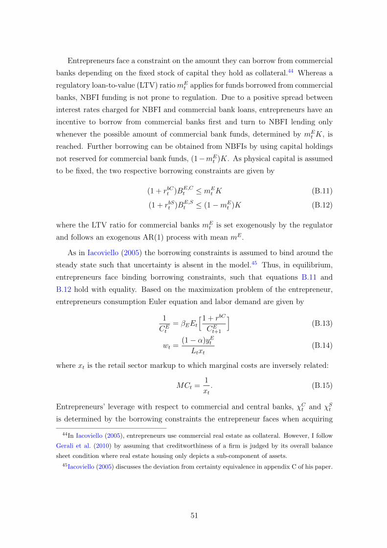
Entrepreneurs face a constraint on the amount of loans BE,Ct (i) they can bor-
row from commercial banks depending on the fixed stock of capital K they hold as
collateral.13 Whereas a regulatory loan-to-value (LTV) ratio mEt applies for funds
borrowed from commercial banks, NBFI funding is not prone to regulation. Due to a
positive spread between interest rates charged for NBFI and commercial bank loans,
entrepreneurs have an incentive to borrow from commercial banks first and turn to
NBFI lending only whenever the possible amount of commercial bank funds, deter-
mined by mEt K, is reached. Further borrowing can be obtained from shadow banks
by using capital holdings not reserved for commercial bank funds, (1−mEt )K.14 As
the stock of physical capital is assumed to be fixed, the two respective borrowing
constraints are given by
(1 + rbCt )BE,Ct ≤ mE
t K (8)
(1 + rbSt )BE,St ≤ (1−mE
t )K (9)
where the LTV ratio for commercial banks mEt is set by a separate regulator in an
exogenous way. In contrast, the LTV ratio applying to NBFI lending, mE,St = 1−mE
t ,
depicts an endogenous variable in the model. As borrowers use the share of capital
not reserved as collateral for commercial bank credit for funding from NBFIs, non-
bank credit may rise if either LTV ratios for commercial bank credit are tightened,
or if the borrowing constraint 8 does not bind. In appendix D, I show how the
introduction of commercial bank market power and resulting commercial bank credit
rationing result in a shift of credit towards NBFIs compared to the efficient steady
13In Iacoviello (2005), entrepreneurs use commercial real estate as collateral. However, I follow
Gerali et al. (2010) by assuming that creditworthiness of a firm is judged by its overall balance
sheet condition where real estate housing only depicts a sub-component of assets.
14See the online appendix of Gebauer and Mazelis (2020) for a detailed analysis.
11
Page 14
state without market power, resulting in a permanent deviation of credit by both
intermediaries from efficient levels.
As in Iacoviello (2005), entrepreneurs face binding borrowing constraints in equi-
librium, such that equations 8 and 9 hold with equality.15 One can furthermore
derive an expression for firm net worth as in Gambacorta and Signoretti (2014)
NWEt = α
yetxt
+K − (1 + rbCt−1)BE,Ct−1 − (1 + rbSt−1)BE,S
t−1 (10)
where firm net worth in period t is given by net revenues minus wage and interest ex-
penses. Finally, as in Gambacorta and Signoretti (2014), entrepreneur consumption
CEt is dependent on firm net worth:
CEt = (1− βE)NWE
t . (11)
3.3 Financial Intermediaries
The financial sector consists of two types of banks, regulated commercial banks
and unregulated NBFIs. Furthermore, commercial banks act under monopolistic
competition in the loan market, whereas NBFIs are perfectly competitive entities,
but constrained by a moral hazard friction arising with the investing household.
3.3.1 Commercial Banks
Following Gebauer and Mazelis (2020) and Gambacorta and Signoretti (2014), com-
mercial banks consist of two agents: A wholesale unit managing the bank’s capital
position and taking deposits from households, and a retail loan entity lending funds
managed by the wholesale unit to entrepreneurs, charging an interest rate markup.16
The wholesale branches of commercial banks operate under perfect competition
and are responsible for the capital position of the respective commercial bank. On
the asset side, they hold funds they provide to the retail loan branch, BE,Ct , earning
the wholesale loan rate rCt . On the liability side, they combine commercial bank net
worth, or capital, KCt , with household deposits, DP,C
t which earn the policy rate rt.
15Iacoviello (2005) discusses the deviation from certainty equivalence in appendix C of his paper.
16In contrast to Gebauer and Mazelis (2020), I do not consider market power in deposit markets
in the model, as monopolistic competition in loan markets is sufficient to derive the key find-
ings. However, the model could straightforwardly be extended by introducing a monopolistically
competitive deposit entity and deposit rate markdowns as in Gebauer and Mazelis (2020).
12
Page 15
Furthermore, the capital position of the wholesale branch is prone to a regulatory
capital requirement, νt. Moving away from the regulatory requirement imposes a
quadratic cost to the bank, which is proportional to the outstanding amount of bank
capital and parameterized by κCk .
The wholesale branch maximization problem can be expressed as
max
BE,Ct , DP,C
t
rCt BE,Ct − rtDP,C
t − κCk2
(KCt
BE,Ct
− νt)2
KCt (12)
subject to the the balance sheet condition
BE,Ct = KC
t +DP,Ct . (13)
The first-order conditions yield the following expression:
rCt = rt − κCk(KCt
BE,Ct
− νt)(
KCt
BE,Ct
)2
. (14)
Aggregate bank capital KCt is accumulated from retained earnings only:
KCt = KC
t−1(1− δC) + JCt (15)
where JCt depicts aggregate commercial bank profits from the two bank branches,
see equation B.26 in appendix B. Capital management costs are captured by δC .
Finally, retail loan branches act under monopolistic competition. They buy
wholesale loans, differentiate them at no cost, and resell them to borrowing en-
trepreneurs. In doing so, the retail loan branch charges a markup µt over the
wholesale loan rate, and the retail loan rate is thus given by
rbCt = rt − κCk(KCt
BE,Ct
− νt)(
KCt
BE,Ct
)2
+ µt. (16)
3.3.2 Non-Bank Financial Institutions
In contrast to the commercial banking sector, NBFIs are not regulated and do not
operate under monopolistic competition. Furthermore, NBFIs’ ability to acquire
external funds is constrained by a moral hazard problem as in Gebauer and Mazelis
(2020) and Gertler and Karadi (2011) that limits the creditors’ willingness to provide
external funds.
NBFIs are assumed to have a finite lifetime: they disappear from the market
after some years, whereas the point of exit is unknown a priori. Each NBFI faces
13
Page 16
an i.i.d. survival probability σS with which he will be operating in the next period,
so his exit probability in period t is 1− σS. Every period new NBFIs enter with an
endowment of wS they receive in the first period of existence, but not thereafter.
The number of NBFIs in the system is constant.
For NBFI j, as long as the real return on lending, (rbSt − rdSt ) is positive, it is
profitable to accumulate capital until he exits the non-bank finance sector. The
NBFI’s objective to maximize expected terminal wealth, vt(j), is given by
vt(j) = maxEt
∞∑i=0
(1− σS)σSiβi+1S KS
t+1+i(j). (17)
As I assume some NBFIs to exit each period and new bankers to enter the market,
aggregate capital KSt is determined by capital of continuing NBFIs, KS,c
t , and capital
of new bankers that enter, KS,nt
KSt = KS,c
t +KS,nt . (18)
Following Gebauer and Mazelis (2020) yields the following law of motion for NBFI
capital:
KSt = σS[(rbSt−1 − rdSt−1)φSt−1 + (1 + rdSt−1)]KS
t−1 + ωSBE,St−1 (19)
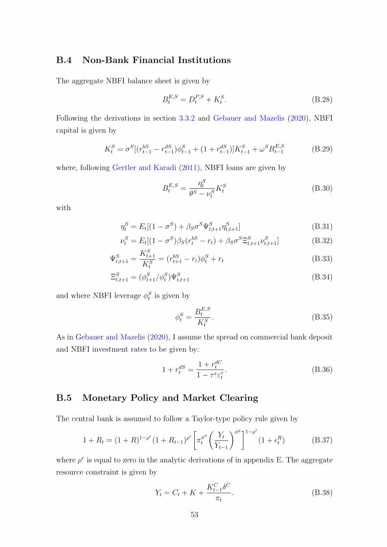
and the aggregate NBFI balance sheet condition is given by
BE,St = DP,S
t +KSt . (20)
Finally, I assume a non-negative spread between the interest rates earned on NBFI
investments, rdSt , and on the deposits households can place with commercial banks,
rdCt , which is determined by the parameter τS, with 0 ≤ τS ≤ 1:17
1 + rdSt =1 + rdCt1− τSετt
. (21)
3.4 Monetary Policy and Market Clearing
The central bank is assumed to follow a Taylor-type policy rule given by
1 +Rt = (1 +R)1−ρr(1 +Rt−1)ρr
[πφ
π
t
(YtYt−1
)φy]1−ρr
(1 + εRt ) (22)
17In the online appendix to Gebauer and Mazelis (2020), a microfoundation for the existence of
a positive spread is provided.
14
Page 17
where ρr is equal to zero in the analytic derivations of appendix E. The model
features sticky prices a la Calvo (1983), which are introduced following Benigno and
Woodford (2005). The aggregate resource constraint is given by
Yt = Ct +K +KCt−1δ
C
πt. (23)
Market clearing implies
Yt = γyyEt (24)
Ct = CPt γp + CE
t γe (25)
Bt = BE,Ct +BE,S
t . (26)
NBFI and commercial bank credit-to-GDP ratios are defined as:
Zt =BE,Ct
Yt(27)
ZSBt =
BE,St
Yt. (28)
Loan and deposit rate spreads paid by commercial bank and NBFIs are given by
∆loant = rbSt − rbCt (29)
∆depositt = rdSt −Rt (30)
and the spreads earned on intermediation by commercial banks and NBFIs by
∆Ct = rbCt −Rt (31)
∆St = rbSt − rdSt . (32)
4 Calibration
Calibrated parameters are largely based on the estimated parameter values in
Gebauer and Mazelis (2020) and shown in table 1.18 In the baseline calibration, the
steady-state commercial bank capital requirement is set to 10.5 percent, in line with
the proposed level in the Basel III framework. The discount factors for households
and firms are calibrated in line with Gerali et al. (2010) and allow for distinguish-
ing between patient households as savers and impatient entrepreneurs as borrowers.
18I compare dynamic simulations under this parameterization with an estimated version of the
actual model described in section 3 in appendix C.
15
Page 18
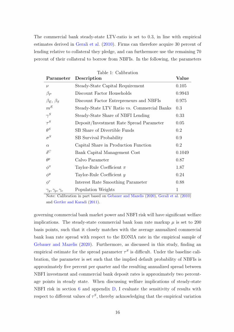
The commercial bank steady-state LTV-ratio is set to 0.3, in line with empirical
estimates derived in Gerali et al. (2010). Firms can therefore acquire 30 percent of
lending relative to collateral they pledge, and can furthermore use the remaining 70
percent of their collateral to borrow from NBFIs. In the following, the parameters
Table 1: CalibrationParameter Description Value
ν Steady-State Capital Requirement 0.105
βP Discount Factor Households 0.9943
βE, βS Discount Factor Entrepreneurs and NBFIs 0.975
mE Steady-State LTV Ratio vs. Commercial Banks 0.3
γS Steady-State Share of NBFI Lending 0.33
τS Deposit/Investment Rate Spread Parameter 0.05
θS SB Share of Divertible Funds 0.2
σS SB Survival Probability 0.9
α Capital Share in Production Function 0.2
δC Bank Capital Management Cost 0.1049
θp Calvo Parameter 0.87
φπ Taylor-Rule Coefficient π 1.87
φy Taylor-Rule Coefficient y 0.24
φr Interest Rate Smoothing Parameter 0.88
γy, γp, γe Population Weights 1
Note: Calibration in part based on Gebauer and Mazelis (2020), Gerali et al. (2010)
and Gertler and Karadi (2011).
governing commercial bank market power and NBFI risk will have significant welfare
implications. The steady-state commercial bank loan rate markup µ is set to 200
basis points, such that it closely matches with the average annualized commercial
bank loan rate spread with respect to the EONIA rate in the empirical sample of
Gebauer and Mazelis (2020). Furthermore, as discussed in this study, finding an
empirical estimate for the spread parameter τS is difficult. Under the baseline cali-
bration, the parameter is set such that the implied default probability of NBFIs is
approximately five percent per quarter and the resulting annualized spread between
NBFI investment and commercial bank deposit rates is approximately two percent-
age points in steady state. When discussing welfare implications of steady-state
NBFI risk in section 6 and appendix D, I evaluate the sensitivity of results with
respect to different values of τS, thereby acknowledging that the empirical variation
16
Page 19
in actual returns and resulting spreads can be large on the micro-level.
Remaining parameters are calibrated such that basic empirical relationships
observed in the euro area data on commercial banking and non-bank finance are
matched.19 NBFI leverage is equal to one third in the baseline calibration, in line
with the share of corporate lending-related activities of shadow-bank type financial
firms relative to their net worth in the data. The overall share of NBFIs in to-
tal lending activity is also set to 33 percent, in line with estimates derived on the
grounds of the empirical data used in the introduction. The remaining parameters
are set as discussed in Gebauer and Mazelis (2020).
5 Welfare Analysis: Loss Functions
In the following, I summarize the derivations of welfare loss functions for the cases
with and without non-bank finance described in detail in appendix E and discuss
welfare-optimal macroprudential regulation both from a static and a dynamic per-
spective. In the iterative substitution of the terms in the utility functions sketched
below, I make use of the Taylor rule as an additional model equation linking the
nominal interest rate to output growth and inflation. Thus, I assume that macropru-
dential policy takes the central bank’s actions as given, and sets policy by assuming
these actions to be conducted in a Taylor-type fashion. Therefore, no coordination
among policy makers is assumed at this point.20
5.1 No Non-Bank Finance
In each case, the welfare function is derived following Benigno and Woodford (2005,
2012) from a second-order approximation of aggregate utility. Following Lambertini
et al. (2013) and Rubio (2011), the social welfare measure is given by a weighted
19See Gebauer and Mazelis (2020).
20Several papers recently deviated from this strict assumption by discussing the case of policy
coordination, either by assuming perfect coordination or in the form of strategic-interaction games,
see for instance Bodenstein et al. (2019), Binder et al. (2018), Gelain and Ilbas (2014), or Beau
et al. (2012). The analysis here could be extended in the same direction, by deriving optimal
monetary and macroprudential policies jointly. However, as I will show in the following, my
analysis will provide scope for policy coordination even without the assumption of jointly-optimal
policy coordination of some form in the first place.
17
Page 20
sum of patient households’ and impatient firms’ welfare functions:21
Wt0 = (1− βP )W Pt0
+ (1− βE)W Et0. (33)
For patient household and entrepreneurs, the respective welfare function is given by
the conditional expectation of lifetime utility at date t0,
W Pt0≈ Et0
∞∑t=t0
βt−t0P [U(CPt , L
Pt )] (34)
and
W Et0≈ Et0
∞∑t=t0
βt−t0E [U(CEt )]. (35)
Starting from a second-order approximation of the patient household’s utility func-
tion in equation 1, one can derive an approximated period welfare measure W Pt :
W Pt = 1
2ψY
2
(8) Y2t + 1
2ψr
2
(4)r2t + 1
2ψν
2
(3)ν2t + 1
2ψz
2
(4)Z2t +
+ ψY(7)Yt + ψπ(4)πt + ψν νt + ψz(2)Zt+
+ covars+ t.i.p.+O3
(36)
where W Pt ≡
UPt −UPUPCP
CP. Hats denote percentage deviations from steady state and the
parameters are given in appendix E.1. The terms covars summarizes the sum of
covariances in equation 36. As in Benigno and Woodford (2005, 2012), t.i.p. covers
terms independent of policy decisions and O3 terms of higher order.
Similarly, a period welfare term for entrepreneurs
WEt = CE
t + (1− σ)1
2(CE
t )2 (37)
can be derived from the second-order approximation of the firm utility function
(equation 6). Finally, the terms for W Pt and WE
t can be used in the approximation
of the period joint welfare function
Wt = (1− βP )W Pt + (1− βE)WE
t . (38)
Using second-order approximations of structural relations in the model, the resulting
loss function can be expressed as
Lt = 12λy
2
Y 2t + 1
2λr
2
r2t + 1
2λz,cb
2
Z2t + 1
2λν
2
ν2t + λz,cbZt. (39)
21Under such a definition, households and firms derive the same level of utility from a constant
consumption stream.
18
Page 21
The period welfare loss depends on the variation of the efficient output gap Yt =
Yt − Y ∗t ,22 the variation in the efficient policy rate gap rt = rt − r∗t , the efficient
commercial bank credit-to-GDP ratio gap Zt = Zt−Z∗t , and the capital requirement
νt. In addition, deviations from the steady-state level of the credit-to-GDP ratio Zt
affect period welfare. The parameters λy2, λr
2, λν
2, λz,cb
2, and λz,cb are determined
by steady-state relationships and the structural parameters.
The derived welfare loss function generally resembles the functions employed
under the “revealed preferences approach” (Binder et al., 2018; Angelini et al., 2014)
in that welfare depends on variations in the output gap, credit-to-GDP, and the
macroprudential policy tool νt. However, even without an explicit a-priori mandate
for policy coordination, the monetary policy tool enters the welfare objective of
the regulator.23 Furthermore, the derived loss function features a level term and
therefore does not only contain purely quadratic terms. In section 6.1, I describe
the role of level terms in period loss functions as an indication of distortionary effects
arising from inefficiencies in the economy related to credit.
5.2 Non-Bank Finance
Whereas the broad structure of the derivation is the same for the model with NBFIs,
I briefly highlight how these institutions enter the welfare analysis.24 The derivation
of the second-order approximation of the patient household’s welfare criterion W Pt
does not change once NBFIs are allowed for in the model. NBFIs enters the over-
all welfare criterion via entrepreneurs, as entrepreneur net worth now depends on
borrowing from both intermediaries (equation B.19). By including NBFI credit via
firm net worth, one can derive a respective loss function for the model with NBFIs
which is given by
L′t = 12λy
2 ′Y 2t + 1
2λr
2 ′r2t + 1
2λz,cb
2 ′Z2t + 1
2λz,sb
2 ′(ZSB
t )2 + 12λν
2
ν2t +
+ λz,cb′Zt + λz,sb
′ZSBt (40)
where ZSBt = ZSB
t − ZSBt∗ depicts the efficient NBFI credit-to-GDP gap, based on
the NBFI credit-to-GDP ratio ZSBt . Due to the inclusion of non-bank finance, the
22Deviations from steady state in the efficient economy absent any frictions are indicated with
asterisks. In such an economy, variations are only determined by exogenous shocks.
23By substituting the approximated Taylor rule, the inflation rate instead of the nominal interest
rate would appear in the loss function, indicating that the policy objectives of both the central
bank and the macroprudential regulator are similar.
24See appendix E.2 for the derivation of the loss function with NBFIs.
19
Page 22
composite parameters in equation 40 take different values compared to the param-
eters in equation 39. Furthermore, the level terms with respect to credit-to-GDP
ratios indicate that both commercial bank and NBFI credit relative to GDP devi-
ate permanently from the optimal level whenever λz,cb′
and λz,sb′
are different from
zero; even when no variations in the objective variables are observed. In section
6.1, I discuss potential reasons for distortionary credit levels and evaluate how these
distortions can be corrected.
5.3 Static Evaluation
Analytic derivations of the coefficients in equations 39 and 40 allow for a computation
of parameter values under the baseline calibration. Table 2 depicts the respective
parameter values on the quadratic terms in the form of “sacrifice ratios”: The
parameters on the quadratic terms related to the capital requirement, the output
gap, the NBFI credit-to-GDP ratio, and the interest rate are expressed relative
to the coefficient on the commercial bank credit-to-GDP ratio. Thus, the relative
importance of other policy objectives vis-a-vis commercial bank credit stabilization
in the welfare criterion can be evaluated. The level term parameters λz,cb, λz,cb′and
λz,sb′
are reported in absolute terms.
Table 2: Loss Function ParametersNo Non-Bank Finance Non-Bank Finance
λy2/λz,cb
2Output Gap 2.72 0.76
λz,sb2/λz,cb
2SB Credit/GDP - 0.92
λr2/λz,cb
2Interest Rate 34.25 12.90
λν2/λz,cb
2Capital Requirement 0.009 0.002
λz,cb CB Credit/GDP level -0.16 -1.33
λz,sb SB Credit/GDP level - 1.52Note: Values of coefficients in equations 39 and 40 under baseline parameterization. See
appendix E for derivations.
Strikingly, the importance of credit stabilization relative to interest rate and out-
put gap stabilization increases substantially once NBFIs enter the model. Whereas
the weight on output gap stabilization is almost three times larger than the weight
on commercial bank credit stabilization in the model without NBFIs, the latter ex-
ceeds the output gap weight in the loss function of the model including non-bank
finance. Also, the weight on commercial bank credit stabilization increases sub-
20
Page 23
stantially relative to the weight on the interest rate objective in the model with
non-bank finance. Furthermore, even though the regulator cannot directly stabilize
NBFI credit, he puts a relatively high weight on its variation when setting policy:
Stabilization of credit in the non-bank financial sector enters with almost the same
weight as commercial bank credit variations. Thus, total credit stabilization plays
a much larger role in the model with non-bank finance compared to the case of
perfectly implementable financial regulation without NBFIs.
Finally, the parameters on commercial bank credit level terms, λz,cb and λz,cb′are
negative in both model versions, whereas the parameter for the NBFI credit level
term λz,sb′is positive under reasonable parameter values. As discussed in more detail
in section 6.1 and appendix D, due to market power and NBFI inefficiencies, steady-
state levels of commercial (shadow) bank credit are below (above) efficient levels
that would prevail in a frictionless economy. Due to these deviations, a marginal
increase (decrease) in commercial (shadow) bank credit has a positive welfare effect
(as losses are reduced). I discuss the existence of level terms in the loss functions
and implications for policy in the following section.
6 Welfare Analysis: Optimal Level Policy
The above loss functions indicate that social welfare not only depends on the ability
of policy makers to stabilize cyclical fluctuations in the target variables. Also, the
permanent levels of commercial bank and NBFI credit have welfare implications.
Thus, the model provides scope that both time-invariant and cyclical macropruden-
tial policies can be welfare-enhancing. In the following, I discuss how financial fric-
tions induce permanent steady-state distortions that provide scope for time-invariant
macroprudential policies. Furthermore, I evaluate how different permanent regula-
tory tools can be employed to resolve the resulting policy trade-off.
6.1 Distortionary Effects of Bank Market Power and NBFI
Inefficiencies
As I discuss in detail in the steady-state analysis of appendix D, financial frictions
in both the commercial banking and NBFI sector result in permanent deviations
of shadow and commercial bank credit from their efficient levels. Due to market
power, commercial banks charge a steady-state markup µ on the credit they pro-
21
Page 24
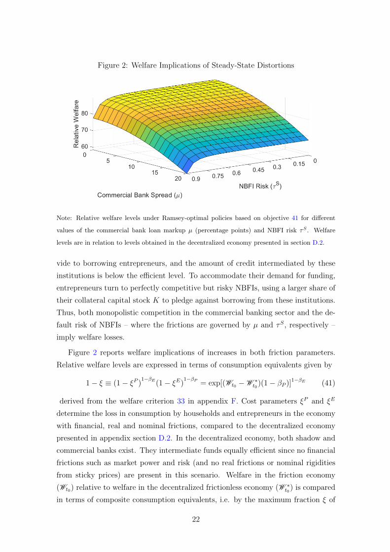
Figure 2: Welfare Implications of Steady-State Distortions
Note: Relative welfare levels under Ramsey-optimal policies based on objective 41 for different
values of the commercial bank loan markup µ (percentage points) and NBFI risk τS . Welfare
levels are in relation to levels obtained in the decentralized economy presented in section D.2.
vide to borrowing entrepreneurs, and the amount of credit intermediated by these
institutions is below the efficient level. To accommodate their demand for funding,
entrepreneurs turn to perfectly competitive but risky NBFIs, using a larger share of
their collateral capital stock K to pledge against borrowing from these institutions.
Thus, both monopolistic competition in the commercial banking sector and the de-
fault risk of NBFIs – where the frictions are governed by µ and τS, respectively –
imply welfare losses.
Figure 2 reports welfare implications of increases in both friction parameters.
Relative welfare levels are expressed in terms of consumption equivalents given by
1− ξ ≡ (1− ξP )1−βE(1− ξE)
1−βP = exp[(Wt0 −W ∗t0
)(1− βP )]1−βE (41)
derived from the welfare criterion 33 in appendix F. Cost parameters ξP and ξE
determine the loss in consumption by households and entrepreneurs in the economy
with financial, real and nominal frictions, compared to the decentralized economy
presented in appendix section D.2. In the decentralized economy, both shadow and
commercial banks exist. They intermediate funds equally efficient since no financial
frictions such as market power and risk (and no real frictions or nominal rigidities
from sticky prices) are present in this scenario. Welfare in the friction economy
(Wt0) relative to welfare in the decentralized frictionless economy (W ∗t0
) is compared
in terms of composite consumption equivalents, i.e. by the maximum fraction ξ of
22
Page 25
consumption that both households and entrepreneurs would be willing to forego in
the economy featuring financial, nominal and real frictions to join the decentralized
economy of appendix D.2. The composite cost ξ is defined such that an increase in
the welfare share of one agent in equation 33 results in a lower contribution of the
other agent’s consumption losses to overall losses, given that 0 < βP , βE < 1.
An increase in the friction parameters results in a reduction of overall welfare in
the model with NBFIs, whereas the amplification of the welfare losses increases for
high levels of distortions in both cases. Particularly for high levels of default risk,
welfare drops sharply. Furthermore, as shown in appendix D.5.1, both frictions imply
that the market-clearing level of time-invariant capital requirements is different in
NBFI and commercial bank credit markets. While the efficient level of capital
requirements in the decentralized economy absent financial frictions
ν∗ =KC
βPmEK(42)
results in clearing of both markets, the levels of steady-state capital requirements
implied by clearing in each credit market – νC and νS, respectively – are given by
νC =KC(1 + βPµ)
βPmEK
νS = KC
[βPK − (1− τS)βP
(1− 1
1 + βPµmE
)K
]−1
(43)
in the steady state featuring financial distortions. As discussed in proposition 6 in
the appendix and shown in the upper part of figure 3, these requirements
1. differ from the efficient level ν∗ in the decentralized frictionless economy
2. increase (decrease) in commercial bank market power (NBFI risk)
The discrepancy in market-clearing levels of permanent capital requirements due
to steady-state distortions has implications for optimal time-invariant macropruden-
tial regulation. As a consequence, it is not feasible to account for both origins of
steady-state distortions with only one macroprudential tool. However, in line with
the Tinbergen (1952) principle, policy makers can pursue a strategy of targeting
credit deviations from socially optimal levels in each lending market separately by
applying one tool to one distortion.
In section D.5.2 of the appendix, I propose that a mix of both supply- and
demand-side oriented time-invariant macroprudential policy tools can lead to allo-
cations where steady-state levels of both commercial bank and NBFI credit are at
23
Page 26
Figure 3: Time-Invariant Levels of Macroprudential Policies
Note: Levels of steady-state capital requirements (νC , νS , ν) and LTV ratios (mE) for different
values of the commercial bank loan markup µ (percentage points) and NBFI risk τS .
24
Page 27
their efficient levels. Capital requirements, targeting credit supply of commercial
banks directly, appear suited to account for distortions stemming from commercial
bank market power. Additionally, whenever NBFI credit supply cannot be regulated
directly, borrower-side tools such as LTV ratios present a means for taking account
of distortions in this market.
In the strategy outlined, the authority responsible for permanent LTV ratios
sets regulation such that the efficiency gap in the NBFI credit market, i.e. the
difference in NBFI credit levels in the distorted steady state and the steady state of
the decentralized economy absent financial frictions given by
BE,S = BE,S −BE,S∗ =
[(1− 1− τS
1 + βPµ
)mE − τS
]KβP (44)
is zero. The implied optimal level of steady-state LTV ratios is then given by
mE = τS1 + βPµ
τS + βPµ. (45)
Conditional on the gap-closing level mE set by the LTV authority, steady-state
capital requirements are chosen such that the commercial bank efficiency gap given
by
BE,C = BE,C −BE,C∗ =
(βP
1 + βPµ− βP
)mEK (46)
is closed. The resulting optimal capital requirement is equal to
ν =KC(τS + βPµ)
βP τSK. (47)
The lower part of figure 3 shows the implied optimal levels of capital requirements
and LTV ratios that close credit gaps stemming from steady-state distortions in the
economy with financial frictions.25 Whenever NBFI risk is almost absent in the
economy (τS → 0), it is optimal for the regulator to set permanent LTV ratios close
to zero, independent of the degree of commercial bank market power (quadrant IV.).
In this case, limiting credit intermediation of monopolistic-competitive commercial
banks and enforcing a shift towards (almost) risk-free NBFIs which act under perfect
competition is beneficial. Similarly, an increase in commercial bank market power
leads to the relative superiority of NBFI credit.
In contrast, higher levels of NBFI risk and lower levels of bank market power
induce an increase in the optimal LTV ratio level, as a welfare-optimal lending
25ν is only defined whenever the NBFI risk parameter τS is positive. Whenever τS = 0, νC = νS
and the efficient level coincides with these expressions (if µ > 0), or with ν∗ (if µ = 0).
25
Page 28
mix features a larger share of commercial bank credit in these cases. Therefore,
lowering borrowing standards with respect to commercial bank lending becomes
beneficial, and in the boundary case of no commercial bank market power, it is
optimal to set LTV ratios to 100 percent, such that all intermediation is conducted by
commercial banks. Similarly, the optimal level of steady-state capital requirements
increases whenever bank market power increases and NBFI risk is low. Again,
tighter regulation for commercial bank is welfare-enhancing whenever NBFI credit
becomes relative more attractive.
6.2 Welfare-Optimal Permanent Capital Requirements
In the previous section, I showed analytically that the existence of commercial bank
market power and NBFI default risk implies a trade-off for policy makers deciding
on the adequate level of commercial bank capital requirements. Quadrant III in
figure 3 indicates that it is optimal for regulators to set capital charges to a high
level in the presence of commercial bank market power to shift intermediation to
the perfectly competitive NBFI sector. However, the presence of NBFI risk induces
welfare losses26 that limit the optimal amount of credit intermediation by these in-
stitutions. Due to the implied trade-off, the optimal level of steady-state capital
requirements is unclear a-priori. Figure 4 shows relative welfare according to equa-
tion 41 under the baseline calibration of µ and τS for different levels of ν. The
optimal level of capital requirements is given by approximately 13.5 percent for the
model with NBFIs, which coincides with the computed value of ν under the baseline
calibration.
Furthermore, independent of the level of capital requirements, welfare levels are
universally lower once NBFI intermediation is taken into account (panel II.), com-
pared to an economy with only commercial bank intermediation (panel I.). Thus,
NBFI risk has adverse welfare implications in the model economy, which are not
compensated by efficiency gains related to non-monopolistic intermediation in the
NBFI sector. Instead, NBFI lending introduces an additional trade-off which com-
plicates welfare-optimal policy making.
Finally, the shape of the welfare profile in figure 4 depends on the presence
of NBFIs. In the absence of NBFIs (panel I.), welfare is relatively high for capi-
26In the model, the actual losses stem from the fact that NBFI profits – which increase in response
to higher intermediation as the leverage constraint of NBFIs is loosened – are not transferred to
households.
26
Page 29
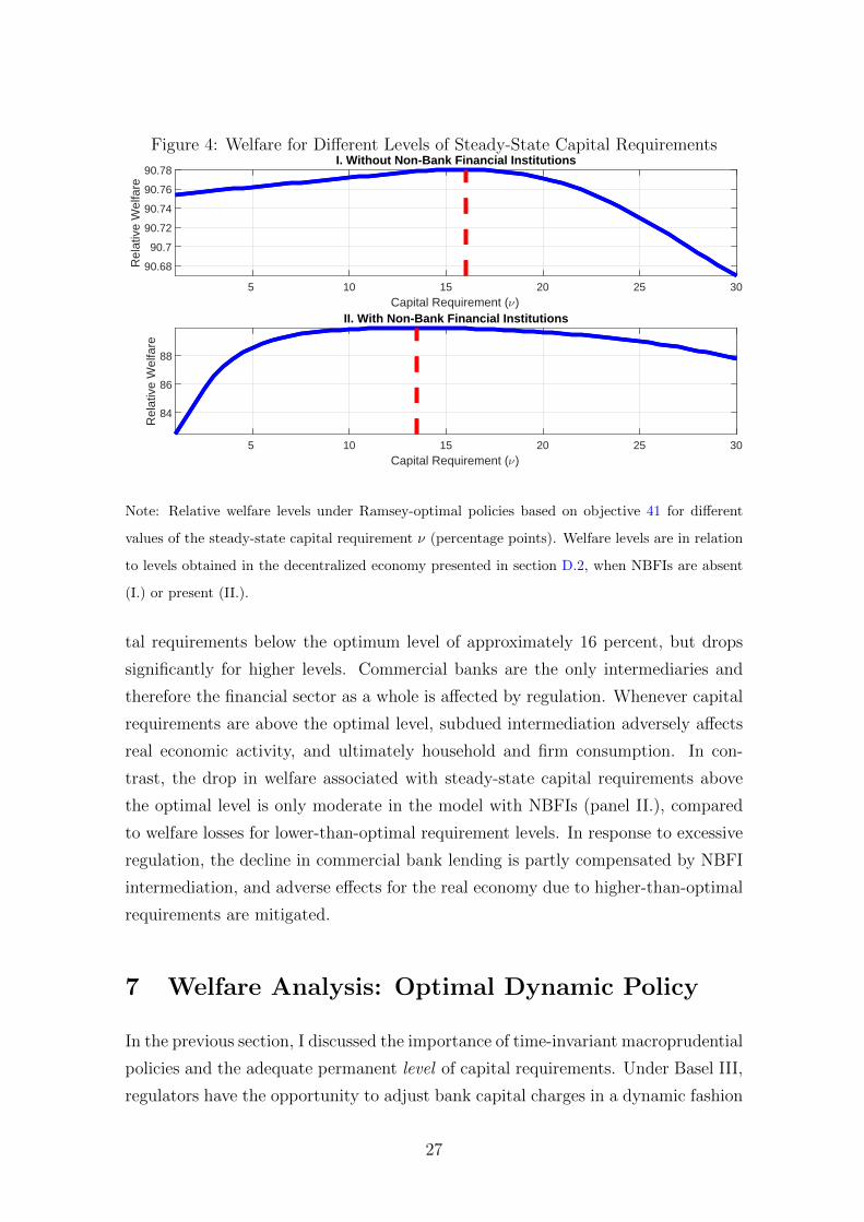
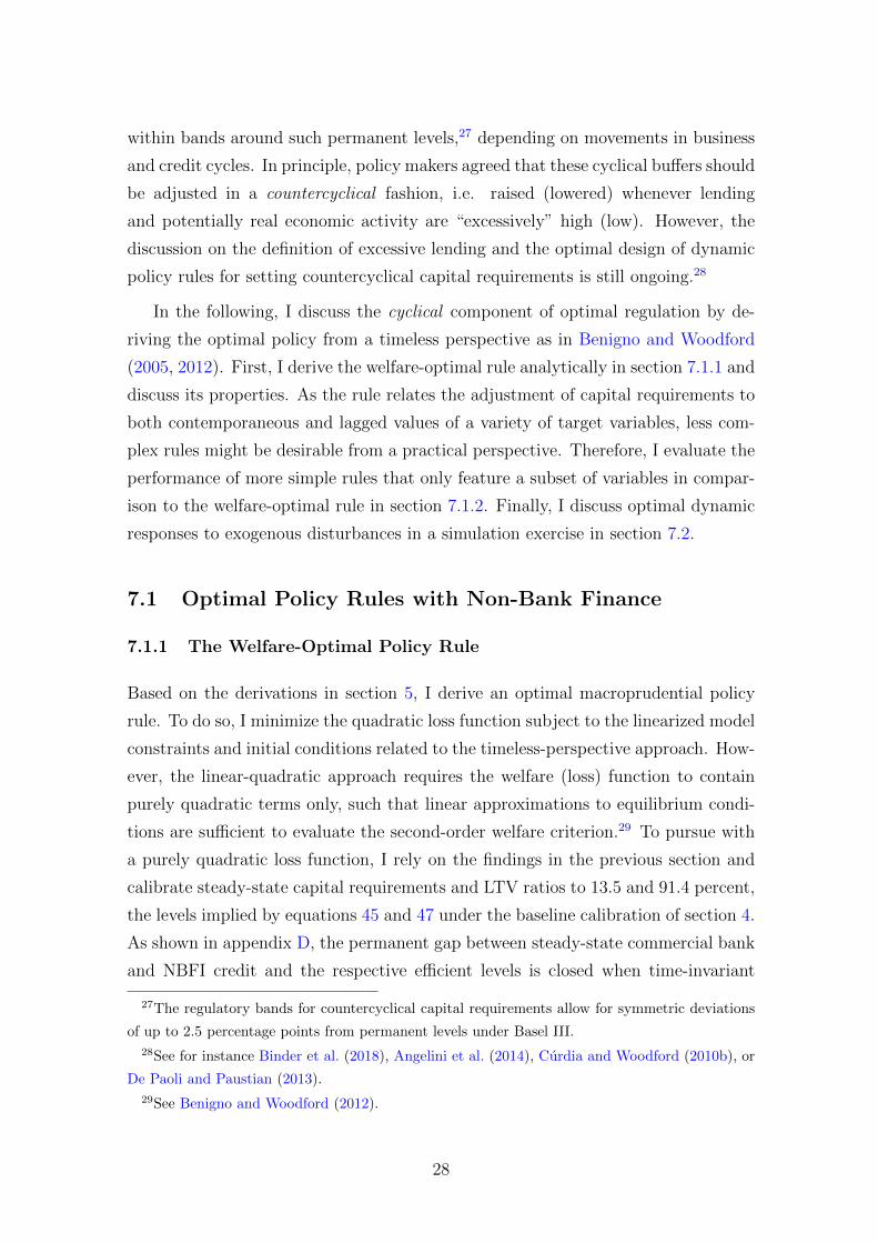
Figure 4: Welfare for Different Levels of Steady-State Capital Requirements
5 10 15 20 25 30Capital Requirement ( )
90.68
90.7
90.72
90.74
90.76
90.78
Rel
ativ
e W
elfa
re
I. Without Non-Bank Financial Institutions
5 10 15 20 25 30Capital Requirement ( )
84
86
88
Rel
ativ
e W
elfa
re
II. With Non-Bank Financial Institutions
Note: Relative welfare levels under Ramsey-optimal policies based on objective 41 for different
values of the steady-state capital requirement ν (percentage points). Welfare levels are in relation
to levels obtained in the decentralized economy presented in section D.2, when NBFIs are absent
(I.) or present (II.).
tal requirements below the optimum level of approximately 16 percent, but drops
significantly for higher levels. Commercial banks are the only intermediaries and
therefore the financial sector as a whole is affected by regulation. Whenever capital
requirements are above the optimal level, subdued intermediation adversely affects
real economic activity, and ultimately household and firm consumption. In con-
trast, the drop in welfare associated with steady-state capital requirements above
the optimal level is only moderate in the model with NBFIs (panel II.), compared
to welfare losses for lower-than-optimal requirement levels. In response to excessive
regulation, the decline in commercial bank lending is partly compensated by NBFI
intermediation, and adverse effects for the real economy due to higher-than-optimal
requirements are mitigated.
7 Welfare Analysis: Optimal Dynamic Policy
In the previous section, I discussed the importance of time-invariant macroprudential
policies and the adequate permanent level of capital requirements. Under Basel III,
regulators have the opportunity to adjust bank capital charges in a dynamic fashion
27
Page 30
within bands around such permanent levels,27 depending on movements in business
and credit cycles. In principle, policy makers agreed that these cyclical buffers should
be adjusted in a countercyclical fashion, i.e. raised (lowered) whenever lending
and potentially real economic activity are “excessively” high (low). However, the
discussion on the definition of excessive lending and the optimal design of dynamic
policy rules for setting countercyclical capital requirements is still ongoing.28
In the following, I discuss the cyclical component of optimal regulation by de-
riving the optimal policy from a timeless perspective as in Benigno and Woodford
(2005, 2012). First, I derive the welfare-optimal rule analytically in section 7.1.1 and
discuss its properties. As the rule relates the adjustment of capital requirements to
both contemporaneous and lagged values of a variety of target variables, less com-
plex rules might be desirable from a practical perspective. Therefore, I evaluate the
performance of more simple rules that only feature a subset of variables in compar-
ison to the welfare-optimal rule in section 7.1.2. Finally, I discuss optimal dynamic
responses to exogenous disturbances in a simulation exercise in section 7.2.
7.1 Optimal Policy Rules with Non-Bank Finance
7.1.1 The Welfare-Optimal Policy Rule
Based on the derivations in section 5, I derive an optimal macroprudential policy
rule. To do so, I minimize the quadratic loss function subject to the linearized model
constraints and initial conditions related to the timeless-perspective approach. How-
ever, the linear-quadratic approach requires the welfare (loss) function to contain
purely quadratic terms only, such that linear approximations to equilibrium condi-
tions are sufficient to evaluate the second-order welfare criterion.29 To pursue with
a purely quadratic loss function, I rely on the findings in the previous section and
calibrate steady-state capital requirements and LTV ratios to 13.5 and 91.4 percent,
the levels implied by equations 45 and 47 under the baseline calibration of section 4.
As shown in appendix D, the permanent gap between steady-state commercial bank
and NBFI credit and the respective efficient levels is closed when time-invariant
27The regulatory bands for countercyclical capital requirements allow for symmetric deviations
of up to 2.5 percentage points from permanent levels under Basel III.
28See for instance Binder et al. (2018), Angelini et al. (2014), Curdia and Woodford (2010b), or
De Paoli and Paustian (2013).
29See Benigno and Woodford (2012).
28
Page 31
macroprudential policies are set to these values, such that the distortionary level
terms Zt and ZSBt in loss function 40 disappear. This allows for the evaluation of
a purely quadratic welfare objective and the derivation of an optimal policy rule
following the LQ-approach of Benigno and Woodford (2005, 2012) and Giannoni
and Woodford (2003a,b). The welfare loss function to be minimized subject to the
log-linearized structural model equations therefore only includes purely quadratic
terms and is given by
L′t = 12λy
2 ′Y 2t + 1
2λr
2 ′r2t + 1
2λz,cb
2 ′Z2t + 1
2λz,sb
2 ′(ZSB
t )2 + 12λν
2 ′ν2t . (48)
Furthermore, as outlined in appendix G, the rule is derived such that Lagrange
multipliers on lagged terms in the first-order conditions of the Ramsey planner
(equations F.2 to F.43 in appendix G) are treated as parameters. Thus, initial
conditions are honoured and not automatically set equal to zero in the minimization
problem of the Ramsey planner. Thus, the time-dependence problem arising in the
implementation of policy in period t0 is taken into account. Therefore, optimal
policy is derived from a timeless perspective,30 and the policy rule describes the
optimal response of the policy maker to random disturbances in all periods t ≥ 0.31
Minimizing loss function 48 subject to the linearized structural equations given
in appendix B and following the iterative approach outlined in appendix G yields
the macroprudential policy rule
νt = ρν + ρν1 νt−1 + ρν2 νt−2 + ρν3 νt−3+ (49)
+ φr1rt + φr2rt−1 + φr3rt−2 + φr4rt−3+
+ φy1Yt + φy2Yt−1 + φy3Yt−2 + φy4Yt−3+
+ φz,cb1 Zt + φz,cb2 Zt−1 + φz,cb3 Zt−2 + φz,cb4 Zt−3+
+ φz,sb1 ZSBt + φz,sb2 ZSB
t−1 + φz,sb3 ZSBt−2 + φz,sb4 ZSB
t−3
where the policy parameters ρν , ρνk, k ∈ 1, 2, 3 and Φmn ,m ∈ r; y; z, cb; z, sb;n ∈
1, 2, 3, 4 are composite parameters consisting of structural parameters and steady-
30By treating initial multiplier conditions as parameters being equal to zero or steady-state
values, I derive optimal policy from a timeless perspective as referred to in Schmitt-Grohe and
Uribe (2005) when the initial multipliers are set to steady-state.
31See for instance Bodenstein et al. (2019), Benigno and Woodford (2005, 2012), Giannoni and
Woodford (2003a,b), or Schmitt-Grohe and Uribe (2005) for extensive discussions on the time-
inconsistency problems arising from neglecting initial conditions and on the derivations of optimal
policy from a timeless perspective for the cases of optimal monetary and fiscal policies.
29
Page 32
state relations.32 In the terminology of Giannoni and Woodford (2003a,b), the rule
given by equation 49 depicts a robustly optimal rule, as none of the derivations out-
lined in appendix G depends on the structural form of the disturbance processes of
the model.33 It is also a robustly optimal direct policy rule, as it does not involve
direct response to exogenous shocks, but to observed target variables only. It is fur-
thermore an implicit policy rule, as contemporaneous values of the target variables
in addition to lagged (predetermined) values enter equation 49, for which contempo-
raneous projections have to be formed implicitly. Table 3 reports parameter values
under the baseline calibration reported in table 1.
Several observations can be drawn from rule 49 and the parameter values un-
der baseline calibration in table 3. First, macroprudential regulators raise capital
requirements under optimal policy whenever the output gap and the commercial
bank credit-to-GDP ratio increase above their efficient levels. Therefore, the op-
timal rule features countercylcical elements usually incorporated in ad-hoc rules
in the “revealed preferences” literature. Whereas the optimal response to output
gap deviations shows some inertia, macroprudential regulators put a high weight
on contemporaneous variations in commercial bank credit-to-GDP. Cumulatively,
the weights associated to these variables are the largest, followed by the cumulative
weight on NBFI credit in absolute terms. Quantitatively, the response to the nom-
inal interest rate is relative moderate in the derived rule, even if the interest rate
weight in loss function 40 turned out to be relatively large (table 2).
Second, the regulator attaches negative weights to deviations in NBFI credit-to-
GDP from efficient levels under optimal policy. Whenever NBFI lending increases
over the efficient level, the macroprudential regulator, ceteris paribus, has a motive
to lower capital requirements for commercial banks to counteract credit leakage.
Thus, the additional trade-off stemming from credit leakage already highlighted
in the evaluation of optimal steady-state levels in section 5.3 is reflected in the
policy rule. Without NBFIs, this trade-off would be absent, and optimal regulation
would unambiguously prescribe higher capital requirements in response to exogenous
shocks that increase credit intermediation – which would then be conducted by
commercial banks only. However, the optimal reaction with NBFIs depends on the
nature of the shock and its relative effect on both credit aggregates, and on the
relative size of the credit coefficients.
32See appendix G where auxiliary parameters defined in the calculations are reported. A full set
of parameters defined in the derivation is available upon request.
33See section B.6 for a description of the assumed shock processes.
30
Page 33
Table 3: Policy Rule Parameters
Parameter Υ = 0 Υ = Υ
Inertia Parameter ρν 0.000 0.092
ρν1 0.562 0.562
ρν2 <0.000 <0.000
ρν3 <0.000 <0.000
Nominal Interest Rate Φr1 -0.030 -0.030
Φr2 -0.027 -0.027
Φr3 -0.059 -0.059
Φr4 -0.031 -0.031
Output Gap Φy1 1.729 1.729
Φy2 1.909 1.909
Φy3 0.156 0.156
Φy4 -0.082 -0.082
CB Credit-to-GDP Φz,cb1 6.103 6.103
Φz,cb2 <0.000 <0.000
Φz,cb3 <0.000 <0.000
Φz,cb4 <0.000 <0.000
SB Credit-to-GDP Φz,sb1 -0.100 -0.100
Φz,sb2 -0.122 -0.122
Φz,sb3 -0.256 -0.256
Φz,sb4 -0.135 -0.135
Note: Values of policy parameters in rule 49 under the
baseline calibration. Υ = 0 (Υ = Υ) when initial con-
ditions given by vector F.44 are equal to zero (equal to
steady state values).
31
Page 34
Third, macroprudential policy responds to movements in the nominal interest
rate, indicating scope for coordination among policy makers. In the model, optimal
macroprudential policy operates to mitigate adverse effects on credit and output, as
capital requirements are loosened whenever the policy rate is raised by the central
bank. As discussed in Gebauer and Mazelis (2020), higher interest rates induce
credit leakage to NBFIs in the model, which provides an additional rationale for
the macroprudential regulator to lower capital requirements in response to tighter
monetary policy. Under optimal policy coordination, these adverse effects would be
considered in the monetary-macroprudential policy trade-off.
Finally, optimal capital regulation for commercial banks appears to be described
by some degree of time-dependence, as both lagged values of the capital requirement
itself and the target variables enter the optimal rule. In some circumstances, pa-
rameter values indicate a stronger weight on past values instead of contemporaneous
projections of target variables. For instance, the response to the output efficiency
gap in t − 1 should be slightly larger than the contemporaneous response. For the
nominal interest rate and NBFI credit, the largest weight is attached to observations
in t − 2. Only in the case of commercial bank credit, the optimal rule indicates a
strong contemporaneous response.
7.1.2 Optimal Simple Rules
In the following, I study whether the complex optimal policy rule 49 can be approx-
imated by simple implementable rules without substantial welfare losses. Following
the “revealed preferences” literature, the generic simple rule is given by:
νt = ρν νt−1 + Φ′Xt (50)
Φ =
φyS
φz,cbS
φz,sbS
Xt =
Yt
Zt
ZSBt
(51)
The macroprudential authority sets the capital requirement νt by considering an
autoregressive component as well as deviations of output and credit-to-GDP gaps
from efficient steady-state levels. Thus, the authority minimizes the loss function 48
by choosing the parameters in Φ, such that the optimization problem is given by:
minΦL′t = 1
2λy
2 ′Y 2t + 1
2λr
2 ′r2t + 1
2λz,cb
2 ′Z2t + 1
2λz,sb
2 ′(ZSB
t )2 + 12λν
2 ′ν2t (52)
s.t. νt = ρν νt−1 + Φ′Xt (53)
0 = Et[f(xt,xt+1,xt−1, θm)] (54)
32
Page 35
where the last line represents constraints arising from the model structure. The
function f(•) refers to the model equations, xt to the vector of endogenous variables,
and θm to the vector of model parameters. Table 4 summarizes the optimized
parameters for different variants of the generic rule 50 which are given by:
OSR/CR 1: νt = φz,cbS Zt (55)
OSR/CR 2: νt = φySYt + φz,cbS Zt (56)
OSR/CR 3: νt = φySYt + φz,cbS Zt + φz,sbS ZSBt (57)
OSR/CR 4: νt = ρν νt−1 + φySYt + φz,cbS Zt + φz,sbS ZSBt (58)
The simplest rule given by equation 55 indicates that the regulator only adjusts capi-
tal requirements in response to a contemporaneous deviation of the commercial bank
credit-to-GDP gap from the efficient steady state. In the rules given by equations
56 to 58, contemporaneous deviations of the output and the NBFI credit-to-GDP
gap as well as an autoregressive term are iteratively introduced.
Table 4: Simple Rule Parameters
Optimal Simple Rules (OSR) Constrained Rules (CR)
Parameter OSR 1 OSR 2 OSR 3 OSR 4 CR 1 CR 2 CR 3 CR 4
ρνS 0.562 0.562
φyS 0.133 0.241 0.243 1.729 1.729 1.729
φz,cbS 12.231 33.169 50.564 52.337 6.103 6.103 6.103 6.103
φz,sbS -11.103 -38.424 -0.100 -0.100
Relative Loss 0.0005 0.0005 0.0003 0.0002 0.0014 1.9915 1.9915 5.5584
Note: Values of policy parameters in rules 55 to 58. Optimal simple rules (OSR) refer to rules
with optimized parameters, while constrained rules (CR) indicate rules with parameters directly
taken from the fully optimal rule 49 under the baseline calibration. Welfare losses under each rule
are expressed relative to welfare losses obtained under the fully optimal policy regime.
The left column of table 4 indicates that for all variants, parameters can be
chosen by the regulator such that the welfare loss relative to the losses obtained
under the welfare-optimal rule 49 is small. However, achieving the same level of
welfare losses with simple rules requires large parameter values in absolute terms.
Neglecting lags and additional variables such as short-term interest rates enforces
stronger reactions to the contemporaneous variables under consideration. Strikingly,
considering credit on a disaggregated level (OSR 3 given by equation 57) results in
a strong increase in the parameter on commercial bank credit compared to simpler
rules, as the sizeable negative coefficient on the NBFI credit-to-GDP gap counteracts
the effect of changes in commercial bank credit.
33
Page 36
The last four columns of table 4 report constrained rules (CR) designed accord-
ing to equations 55 to 58, but without optimized coefficients. Instead, coefficients on
contemporaneous variables are fixed at the respective coefficient values derived for
the fully optimal rule 49 reported in table 3. By incorporating additional contempo-
raneous variables (moving from CR 1 to CR 4) in the constrained rule, the relative
welfare loss increases. Thus, even by incorporating more information in policy rules,
welfare losses can increase if simple rule parameters are not separately optimized.
7.2 Simulation Analysis
As indicated in the previous section, the optimal dynamic policy response to exoge-
nous disturbances particularly depends on movements in both NBFI and commercial
bank credit. In the following simulation exercise, I evaluate how the introduction
of NBFIs alters the policy makers’ ability to stabilize both the financial sector and
real economic activity in response to exogenous macroeconomic shocks. Figures 5
and 6 show welfare-optimal dynamic responses to an unexpected tightening in mon-
etary policy (aggregate demand shock) and to an exogenous improvement of firms’
production technology (aggregate supply shock).34 I simulate these responses under
optimal policy for the cases with (blue lines) and without non-bank finance (red
dashed lines). Furthermore, I consider a scenario with NBFIs where capital require-
ments are not dynamically adjusted, but kept at the optimal steady-state level of
13.5 percent (black dotted lines).
The impulse responses allow for several observations. First, optimal dynamic
macroprudential regulation is effective in stabilizing commercial bank credit, both
in the presence and absence of NBFIs. However, even under optimal policy, the
regulator is not able to completely neutralize credit leakage to NBFIs in response to
macroeconomic shocks. As in Gebauer and Mazelis (2020), unexpected monetary
policy tightening induces a shift of credit intermediation towards NBFIs.35 However,
the quantitative effects of credit leakage are smaller compared to the response under
the ad-hoc policy rules discussed in the previous section. Similarly, an unexpected
positive technology shock increases entrepreneurs’ production income and ultimately
induces borrowing constraint 8 to be less binding. Lower credit constraints with
34In appendix section C, I provide the same set of optimal impulse responses for an estimated
version of the model for comparison.
35Several studies found empirical evidence for credit leakage towards non-bank institutions in
response to monetary policy shocks. See Gebauer and Mazelis (2020).
34
Page 37
Figure 5: Impulse Response Functions Monetary Policy Shock: Different Policy
Scenarios
5 10 15Quarters
-0.1
-0.05
0
0.05
% D
ev.
CB Lending
5 10 15Quarters
0
0.1
0.2
% D
ev.
NBFI Lending
5 10 15Quarters
-40
-20
0
% D
ev.
Capital Requirements
5 10 15Quarters
-0.4
-0.2
0
% D
ev.
Output
5 10 15Quarters
-0.2
-0.1
0
Abs
. Dev
.
Inflation
5 10 15Quarters
0
0.05
0.1
Abs
. Dev
.
Policy Rate
5 10 15Quarters
-0.2
-0.1
0
Abs
. Dev
.
CB Spread
5 10 15Quarters
-0.3
-0.2
-0.1
0
Abs
. Dev
.
NBFI Spread
5 10 15Quarters
-0.3
-0.2
-0.1
0A
bs. D
ev.
Loan Rate Spread
5 10 15Quarters
-0.4
-0.2
0
% D
ev.
HH Consumption
5 10 15Quarters
-1
-0.5
0
0.5
% D
ev.
Firm Consumption
5 10 15Quarters
-0.1
0
0.1
0.2
% D
ev.
CB Capital
5 10 15Quarters
-0.2
-0.1
0
% D
ev.
CB Deposits
5 10 15Quarters
0
0.2
0.4
% D
ev.
NBFI Deposits
5 10 15Quarters
-2
0
2
% D
ev.
CB Profits
Optimal Policy Optimal Policy No NBFIs Permanent Capital Requirements
Note: Impulse responses to a one-standard-deviation monetary policy shock with welfare-optimal
response by macroprudential regulator. Rates in absolute deviations from steady state, all other
variables as percentage deviations from steady state.
35
Page 38
Figure 6: Impulse Response Functions Technology Shock: Different Policy Scenarios
5 10 15Quarters
-0.1
0
0.1
% D
ev.
CB Lending
5 10 15Quarters
-0.2
0
0.2
% D
ev.
NBFI Lending
5 10 15Quarters
0
20
40
% D
ev.
Capital Requirements
5 10 15Quarters
0
0.2
0.4
% D
ev.
Output
5 10 15Quarters
-0.4
-0.2
0
Abs
. Dev
.
Inflation
5 10 15Quarters
-0.2
-0.1
0
Abs
. Dev
.
Policy Rate
5 10 15Quarters
0
0.1
0.2
Abs
. Dev
.
CB Spread
5 10 15Quarters
-0.1
0
0.1
0.2
Abs
. Dev
.
NBFI Spread
5 10 15Quarters
0
0.2
0.4
Abs
. Dev
.
Loan Rate Spread
5 10 15Quarters
0
0.2
0.4
% D
ev.
HH Consumption
5 10 15Quarters
-0.5
0
0.5
1
% D
ev.
Firm Consumption
5 10 15Quarters
-0.2
0
0.2
% D
ev.
CB Capital
5 10 15Quarters
-0.1
0
0.1
0.2
% D
ev.
CB Deposits
5 10 15Quarters
-1
0
1
% D
ev.
NBFI Deposits
5 10 15Quarters
-2
-1
0
% D
ev.
CB Profits
Optimal Policy Optimal Policy No NBFIs Permanent Capital Requirements
Note: Impulse responses to a one-standard-deviation technology shock with welfare-optimal re-
sponse by macroprudential regulator. Rates in absolute deviations from steady state, all other
variables as percentage deviations from steady state.
36
Page 39
respect to commercial bank credit in turn reduce entrepreneurs necessity to turn to
NBFI creditors, such that the share of credit intermediated by commercial banks
increases.
Second, capital requirements are adjusted countercyclically in response to
macroeconomic shocks. In the case of an adverse demand shock (a monetary pol-
icy tightening), regulators lower capital requirements to stabilize commercial bank
credit. Equally, an accommodative supply shock (positive technology shock) induces
regulators to tighten commercial credit requirements to stabilize credit.
Third, and in line with policy rule 49, disturbances resulting in credit leakage,
i.e. in inverse responses of commercial bank and NBFI credit, induce regulators to
adjust capital requirements more aggressively in the presence of non-bank finance.
In response to an unexpected monetary policy tightening, the regulator immedi-
ately decreases capital requirements by approximately 25 percent – which implies a
decrease from 13.5 percent in the optimal steady state to 10.1 percent – whenever
NBFIs are present. In the scenario with commercial banks only, capital requirements
decrease by only 18 percent – from 13.5 to 11.1 percent – on impact.
Consequently, implications of non-bank finance for cyclical macroprudential pol-
icy crucially depend on the direction in which commercial bank and NBFI credit
move in response to disturbances. As discussed in the previous section, macroe-
conomic disturbances leading to the same direction of commercial bank and NBFI
credit responses provide a motive for mitigating the regulatory response to com-
mercial bank credit.36 In contrast, the presence of credit leakage leading to inverse
credit responses provides a rationale for a stronger policy response.
Fourth, the results for both monetary policy and technology shocks indicate
that optimal capital regulation – while suited to stabilize commercial bank credit
intermediation – fails to stabilize the output gap efficiently in response to macroe-
conomic shocks. Even more, the additional policy trade-off between bank market
power and NBFI risk mitigates the ability of regulators to stabilize the output gap in
the presence of NBFIs, compared to the case where they can fully reach a homoge-
36The finding is also in line with results from the counterfactual simulation in Gebauer and
Mazelis (2020). However, while the ad-hoc rules employed there do consider movements in overall
credit, they do not feature the credit leakage motive of optimal policy. Still, as shown in Gebauer
and Mazelis (2020), regulators concerned with overall credit would have tightened requirements less
strongly in the years preceding the financial crisis – a period of growth in both commercial bank
and NBFI credit (figure 1) – compared to regulators that would have only considered commercial
bank credit.
37
Page 40
neous financial sector with their policies. In both scenarios, the direct link between
macroprudential regulation and commercial bank credit allows regulators to stabilize
commercial bank activity efficiently, while NBFI intermediation and real economic
activity are only partly stabilized. Therefore, while capital requirements might be
suited to directly target volatility in commercial bank intermediation, additional
policies targeting business cycle fluctuations or non-bank finance more directly are
likely to increase economic and financial stability and to provide even further welfare
improvements.
Fifth, regulators are particularly efficient in stabilizing commercial bank credit
under dynamic optimal policy. Under the fixed-requirement scenario (black dot-
ted line), an unexpected increase in the policy rate leads to a rise in deposit and
commercial bank loan rates. In turn, higher commercial bank credit costs reduce
lending by commercial banks (figure 5). NBFI lending increases slightly more com-
pared to the optimal policy scenario, as the spread between NBFI and commercial
bank loan rates decreases. Furthermore, the drop in output and inflation is stronger
under fixed capital requirements, even though the difference in the responses is rela-
tively small in both scenarios. Welfare-optimal adjustments of capital requirements
therefore provide only limited additional stabilization of business cycles, confirming
the above findings. Again, the adjustment of capital requirements has a particular
impact on commercial bank activities, as these institutions are directly affected.
Similarly, the unexpected productivity shock depicted in figure 6 results in an
increase in commercial bank lending whenever capital requirements are fixed, while
commercial bank credit is almost completely stabilized under the welfare-optimal
policy. Again, an increase in capital requirements by 26 percent – from 13.5 to 17
percent – only mildly affects business cycle dynamics but has substantial impact on
commercial banks’ activity.
8 Conclusion
In this paper, I study optimal macroprudential regulation for commercial banks in
the presence of unregulated non-bank financial intermediaries (NBFIs). I analyti-
cally derive welfare-optimal policies under commitment in a New Keynesian DSGE
model featuring both intermediaries based on different microfoundations. I com-
pare my findings to a scenario where the financial sector only consists of regulated
commercial banks.
38
Page 41
The derived period loss functions resemble ad-hoc welfare criteria usually em-
ployed in the “revealed preferences” approach towards optimal macroprudential pol-
icy. However, in addition to output- and credit-related terms, they also include a
stabilization criterion with respect to nominal short-term interest rates. Thus, even
without an a-priori assumption on policy coordination, I find potential welfare gains
from cooperation between monetary and macroprudential authorities.
Due to commercial bank market power and NBFI riskiness, steady-state lending
by both intermediaries permanently deviates from efficient levels: Commercial bank
lending is below the optimal level, and NBFI intermediation is higher in the distorted
steady state. While bank capital regulation alone cannot mitigate inefficiencies in
both credit markets, I show that a combination of static capital requirements and
LTV ratios can resolve both steady-state distortions. The welfare-optimal level of
permanent capital requirements is 13.5 percent in the model including NBFIs, com-
pared to 16 percent in a model where commercial banks are the only lenders. Raising
capital requirements induces a shift of intermediation towards risky NBFIs, as the
relative cost of commercial bank credit increases with tighter capital regulation.
Thus, by neglecting credit leakage to NBFIs, the costs from tightening regulation
are not fully internalized by regulators.
Finally, non-bank finance affects the optimal dynamic response of macropru-
dential regulation to fluctuations in output and credit. Whenever macroeconomic
disturbances imply credit leakage towards NBFIs, regulatory adjustments are larger
than in a model without NBFIs. For instance, after an unexpected increase in the
policy rate by annualized 40 basis points, capital requirements decrease from 13.5
percent to 10.1 percent in the presence of non-bank finance. In the scenario without
NBFIs, capital requirements decrease to only 11.1 percent.
My findings indicate that neglecting NBFIs potentially impairs the efficiency
of macroprudential policies, as regulators do not internalize credit leakage and the
trade-off related to the composition of credit. Thus, they should consider develop-
ments in the non-bank financial sector, even if their policies only apply to traditional
banks. Furthermore, the lack of macroprudential tools for NBFIs raises potential
gains from coordinating different macroprudential measures. In addition, coordina-
tion with monetary policy can play a role, as NBFIs’ activity is also related to the
overall price of credit in the economy. Thus, nominal interest rate levels matter, and
credit leakage may be aggravated when the effective lower bound (ELB) on nominal
interest rates is reached.
39
Page 42
References
Acharya, V. V., Schnabl, P., and Suarez, G. (2013). Securitization Without Risk
Transfer. Journal of Financial Economics, 107(3):515–536.
Adrian, T. (2014). Financial Stability Policies for Shadow Banking. Federal Reserve
Bank of New York Staff Report, (664).
Adrian, T. and Ashcraft, A. B. (2012). Shadow Banking Regulation. Annual Review
of Financial Economics, 4:99–140.
Adrian, T. and Ashcraft, A. B. (2016). Shadow Banking: A Review of the Literature.
In G., J., editor, Banking Crises. Palgrave Macmillan, London.
Adrian, T. and Jones, B. (2018). Shadow Banking and Market-Based Finance. In
Financial Stability Review April 2018. Banque de France.
Adrian, T. and Liang, N. (2016). Monetary Policy, Financial Conditions, and Fi-
nancial Stability. CEPR Discussion Paper, (DP11394).
Aguilar, P., Hurtado, S., Fahr, S., and Gerba, E. (2019). Quest for Robust Optimal
Macroprudential Policy. Bank of Spain Working Paper Series, (1916).
Aikman, D., Giese, J., Kapadia, S., and McLeay, M. (2018). Targeting Financial
Stability: Macroprudential or Monetary Policy? Bank of England Staff Working
Paper, (734).
Aiyar, S., Calomiris, C. W., and Wieladek, T. (2016). How Does Credit Supply Re-
spond to Monetary Policy and Bank Minimum Capital Requirements? European
Economic Review, 82:142–165.
Allen, F. and Gale, D. (2000). Financial Contagion. Journal of Political Economy,
108(1):1–33.
Angelini, P., Neri, S., and Panetta, F. (2014). The Interaction between Capital
Requirements and Monetary Policy. Journal of Money, Credit and Banking,
46(6):1073–1112.
Angeloni, I. and Faia, E. (2013). Capital Regulation and Monetary Policy with
Fragile Banks. Journal of Monetary Economics, 60(2013):311–324.
40
Page 43
Bakk-Simon, K., Borgioli, S., Giron, C., Hempell, H., Maddaloni, A., Recine, F.,
and Rosati, S. (2012). Shadow Banking in the Euro Area - An Overview. ECB
Occasional Paper Series, (133).
Bean, C., Paustian, M., Penalver, A., and Taylor, T. (2010). Monetary Policy After
the Fall. Bank of England Working Paper.
Beau, D., Clerc, L., and Mojon, B. (2012). Macro-Prudential Policy and the Conduct
of Monetary Policy. Banque de France Working Paper, (390).
Begenau, J. and Landvoigt, T. (2016). Financial Regulation in a Quantitative Model
of the Modern Banking System. Working Paper.
Benigno, P. and Woodford, M. (2005). Inflation Stabilization and Welfare: The
Case of a Distorted Steady State. Journal of the European Economic Association,
3(6):1185–1236.
Benigno, P. and Woodford, M. (2012). Linear-Quadratic Approximation of Optimal
Policy Problems. Journal of Economic Theory, 147:1–42.
Berger, A. N., Demirguc-Kunt, A., Levine, R., and Haubrich, J. G. (2004). Concen-
tration and Competition: An Evolution in the Making. Journal of Money, Credit
and Banking, 36(4):433–451.
Binder, M., Lieberknecht, P., Quintana, J., and Wieland, V. (2018). Robust
Macroprudential Policy Rules under Model Uncertainty. Annual Conference 2018
(Freiburg, Breisgau): Digital Economy 181503, Verein fur Socialpolitik / German
Economic Association.
Bodenstein, M., Guerrieri, L., and LaBriola, J. (2019). Macroeconomic Policy
Games. Journal of Monetary Economics, 101:64–81.
Borio, C. (2003). Towards a Macroprudential Framework for Financial Supervision
and Regulation? CESifo Economic Studies, 49(2):181–215.
Borio, C. (2009). Implementing the Macroprudential Approach to Financial Regu-
lation and Supervision. Financial Stability Review, 13:31–41.
Borio, C. (2011). Rediscovering the Macroeconomic Roots of Financial Stability
Policy: Journey, Challenges, and a Way Forward. Annual Review of Financial
Economics, 3(1):87–117.
41
Page 44
Borio, C. and Shim, I. (2007). What Can (Macro)-Prudential Policy do to Support
Monetary Policy? BIS Working Papers, 242.
Bundesbank (2014). The Shadow Bankning System in the Euro Area: Overview and
Monetary Policy Implications. Deutsche Bundesbank Monthly Report, (March).
Calvo, G. A. (1983). Staggered Prices in a Utility-Maximizing Framework. Journal
of Monetary Economics, 12(3):383–398.
Chen, N.-K. (2001). Bank Net Worth, Asset Prices and Economic Activity. Journal
of Monetary Economics, 48(2001):415–436.
Christensen, I., Meh, C., and Moran, K. (2011). Bank Leverage Regulation and
Macroeconomic Dynamics. Bank of Canada Working Paper, (2011-32).
Christiano, L. J., Eichenbaum, M. S., and Trabandt, M. (2018). On DSGE Models.
Journal of Economic Perspectives, 32(3):113–140.
Claessens, S. and Laeven, L. (2004). What Drives Bank Competition? Some Inter-
national Evidence. Journal of Money, Credit and Banking, 36(3):563–583.
Clerc, L., Derviz, A., Mendicino, C., Moyen, S., Nikolov, K., Stracca, L., Suarez, J.,
and Vardoulakis, A. (2015). Capital Regulation in a Macroeconomic Model with
Three Layers of Default. Banque de France Working Paper, (533).
Collard, F., Dellas, H., Diba, B., and Loisel, O. (2014). Optimal Monetary and
Prudential Policies. Banque de France Working Paper, (413).
Curdia, V. and Woodford, M. (2010a). Conventional and Unconventional Monetary
Policy. Federal Reserve Bank of St. Louis Review, 92:229–264.
Curdia, V. and Woodford, M. (2010b). Credit Spreads and Monetary Policy. Journal
of Money, Credit and Banking, 42(s1):3–35.
Curdia, V. and Woodford, M. (2011). The Central-Bank Balance Sheet as an In-
strument of Monetary Policy. Journal of Monetary Economics, 58(1):54–79.
De Bandt, O. and Davis, E. P. (2000). Competition, Contestability and Market
Structure in European Banking Sectors on the Eve of EMU. Journal of Banking
and Finance, 24(6):1045–1066.
42
Page 45
De Jonghe, O., Dewachter, H., and Ongena, S. (2020). Bank Capital (Requirements)
and Credit Supply: Evidence from Pillar 2 Decisions. Journal of Corporate Fi-
nance, 60:101518.
De Paoli, B. and Paustian, M. (2013). Coordinating Monetary and Macroprudential
Policies. Federal Reserve Bank of New York Staff Report, (653).
Degryse, H. and Ongena, S. (2008). Competition and Regulation in the Banking
Sector: A Review of the Empirical Evidence on the Sources of Bank Rates. In
Boot, A. and Thakor, A., editors, Handbook of Financial Intermediation and
Banking. Elsevier.
Doyle, N., Hermans, L., Molitor, P., and Weistroffer, C. (2016). Shadow Banking
in the Euro Area: Risks and Vulnerabilities in the Investment Fund Sector. ECB
Occasional Paper Series, (174).
Farhi, E. and Tirole, J. (2017). Shadow Banking and the Four Pillars of Traditional
Financial Intermediation. NBER Working Paper, (23930).
Ferrero, A., Harrison, R., and Nelson, B. (2018). Concerted Efforts? Monetary
Policy and Macro-Prudential Tools. Bank of England Working Paper, (727).
Feve, P. and Pierrard, O. (2017). Financial Regulation and Shadow Banking: A
Small-Scale DSGE Perspective. TSE Working Paper, 17-829.
Gambacorta, L. and Signoretti, F. M. (2014). Should Monetary Policy Lean Against
the Wind?: An Analysis Based on a DSGE Model With Banking. Journal of
Economic Dynamics and Control, 43(June):146–174.
Gebauer, S. and Mazelis, F. (2020). Macroprudential Regulation and Leakage to
the Shadow Banking Sector. ECB Working Paper Series, (2407).
Gelain, P. and Ilbas, P. (2014). Monetary and Macroprudential Policies in an Esti-
mated Model with Financial Intermediation. National Bank of Belgium Working
Paper, (258).
Gennaioli, N., Shleifer, A., and Vishny, R. W. (2013). A Model of Shadow Banking.
Journal of Finance, 68(4):1331–1363.
Gerali, A., Neri, S., Sessa, L., and Signoretti, F. M. (2010). Credit and Banking
in a DSGE Model for the Euro Area. Journal of Money, Credit and Banking,
42(1):107–141.
43
Page 46
Gertler, M. and Karadi, P. (2011). A Model of Unconventional Monetary Policy.
Journal of Monetary Economics, 58(1):17–34.
Gertler, M. and Kiyotaki, N. (2011). Financial Intermediation and Credit Policy in
Business Cycle Analysis. In Friedman, B. M. and Woodford, M., editors, Handbook
of Monetary Economics. Elsevier.
Gertler, M. and Kiyotaki, N. (2015). Banking, Liquidity, and Bank Runs in an
Infinite Horizon Economy. American Economic Review, 105(7):2011–2043.
Gertler, M., Kiyotaki, N., and Prestipino, A. (2016). Wholesale Banking and Bank
Runs in Macroeconomic Modelling of Financial Crises. In Taylor, J. B. and Uhlig,
H., editors, Handbook of Macroeconomics. Elsevier.
Giannoni, M. P. and Woodford, M. (2003a). Optimal Interest-Rate Rules: I. General
Theory. NBER Working Paper, (9419).
Giannoni, M. P. and Woodford, M. (2003b). Optimal Interest-Rate Rules: II. Ap-
plications. NBER Working Paper, (9420).
Harris, M., Opp, C. C., and Opp, M. M. (2014). Higher Capital Requirements,
Safer Banks? - Macroprudential Regulation in a Competitive Financial System.
Chicago Booth Working Paper.
Holstrom, B. and Tirole, J. (1997). Financial Intermediation, Loanable Funds, and
the Real Sector. The Quarterly Journal of Economics, 112(3):663–691.
Iacoviello, M. (2005). House Prices, Borrowing Constraints, and Monetary Policy
in the Business Cycle. American Economic Review, 95(3):739–764.
Iacoviello, M. and Guerrieri, L. (2017). Collateral Constraints and Macroeconomic
Asymmetries. Journal of Monetary Economics, 90:28–49.
Kiyotaki, N. and Moore, J. (2012). Liquidity, Business Cycles, and Monetary Policy.
NBER Working Paper, (17934).
Kroszner, R. (2010). Interconnectedness, Fragility and the Financial Crisis. In
Mimeograph The University of Chicago Booth School of Business, prepared for
Financial Crisis Forum Financial Crisis Inquiry Commission, Washington DC,
February.
44
Page 47
Lambertini, L., Mendicino, C., and Punzi, M. T. (2013). Leaning Against
Boom–Bust Cycles in Credit and Housing Prices. Journal of Economic Dynamics
and Control, 37:1500–1522.
Mazelis, F. (2016). Implications of Shadow Bank Regulation for Monetary Policy
at the Zero Lower Bound. Working Paper.
Meeks, R. (2017). Capital Regulation and the Macroeconomy: Empirical Evidence
and Macroprudential Policy. European Economic Review, 95:125–141.
Meeks, R. and Nelson, B. (2017). Shadow Banks and Macroeconomic Instability.
Journal of Money, Credit and Banking, 49(1):1483–1516.
Meh, C. and Moran, K. (2010). The Role of Bank Capital in the Propagation of
Shocks. Journal of Economic Dynamics and Control, 34(3):555–576.
Ordonez, G. (2018). Sustainable Shadow Banking. American Economic Journal:
Macroeconomics, 10(1):33–56.
Pires, F. (2019). Non-Banks in the EU: Ensuring a Smooth Transition to a Capital
Markets Union. SUERF Policy Note, (103).
Plantin, G. (2015). Shadow Banking and Bank Capital Regulation. Review of
Financial Studies, 28(1):146–175.
Poeschl, J. (2020). The Macroeconomic Effects of Shadow Banking Panics. Working
Paper.
Pozsar, Z., Adrian, T., Ashcraft, A., and Boesky, H. (2010). Shadow Banking.
Federal Reserve Bank of New York Staff Report, (458).
Rubio, M. (2011). Fixed- and Variable-Rate Mortgages, Business Cycles, and Mon-
etary Policy. Journal of Money, Credit and Banking, 43(4):657–688.
Schmitt-Grohe, S. and Uribe, M. (2005). Optimal Fiscal and Monetary Policy in a
Medium-Scale Macroeconomic Model. NBER Macroeconomic Annual 2005.
Silvo, A. (2015). The Interaction of Monetary and Macroprudential Policies in
Economic Stabilisation. HECER Discussion Papers, (395).
Stein, J. C. (2013). Overheating in credit markets: Origins, measurement and policy
responses. Remarks at a Research Symposium sponsored by the Federal Reserve
Bank of St. Louis.
45
Page 48
Tinbergen, J. (1952). On the Theory of Economic Policy. Amsterdam.
Verona, F., Martins, M. M., and Drumond, I. (2013). (Un)anticipated Monetary
Policy in a DSGE Model with a Shadow Banking System. International Journal
of Central Banking, 9(3):78–124.
Woodford, M. (2011). Optimal Monetary Stabilization Policy. In Friedman, B. M.
and Woodford, M., editors, Handbook of Monetary Economics. Elsevier.
46
Page 49
A The Role of Non-Banks for Regulation
The increasing importance of non-bank financial intermediation and the resulting
relevance for financial stability has recently been recognized by supervisors. How-
ever, designing a macroprudential framework for the non-bank financial sector sim-
ilar to the approach introduced for commercial banks is barely feasible. While
traditional banks usually intermediate funds between borrowers and savers in a uni-
versal fashion, a multitude of specialized financial corporations operating in a com-
plex intermediation chain are usually involved in non-bank credit intermediation.37
Therefore, NBFI regulation is largely limited to microprudential approaches or spe-
cial regulative measures that can be introduced for a set of institutions involved in
credit intermediation.38
Nevertheless, changes in regulation for the commercial banking sector can trigger
a shift of credit intermediation towards less regulated parts of the financial system.
In a scenario with only commercial banks, the trade-off the regulator faces arises
from the contemporaneous stabilization of credit and economic activity (figure 7):39
Since the regulator’s policy applies to the whole financial system in such a (counter-
factual) scenario, changes in capital requirements affect total credit intermediation.
Therefore, higher capital requirements can directly result – given that bank capi-
tal barely adjusts in the short run – in a reduction of credit intermediation, as all
financial intermediaries in the economy have to reduce their assets to oblige with
the regulatory requirement.40 Lower credit intermediation potentially comes at the
expense of lower economic activity, and the regulator has to decide on the optimal
capital requirement level to balance the benefits of reduced lending activity and thus
(potentially) higher financial stability with the cost of lower output growth.
37See for instance Adrian (2014), Adrian and Liang (2016), or Pozsar et al. (2010) for a discussion
of the shadow bank intermediation chain.
38In Europe, the updated Markets in Financial Instruments Directive (MiFID II/MiFIR) aims
at increasing transparency and investor protection in market-based finance, thereby applying to
a subset of institutions under the broad definition of NBFIs used here. However, the approach
primarily focuses on the harmonization of reporting and conduct of business standards and autho-
rization requirements. Explicit capital requirements, affecting the non-bank financial sector as a
whole, are not part of the regulatory package.
39See for instance Angelini et al. (2014) or Binder et al. (2018).
40There is ample empirical evidence that a tightening of capital regulation is usually associated
with a decline in lending by financial intermediaries. See for instance De Jonghe et al. (2020),
Meeks (2017), or Aiyar et al. (2016).
47
Page 50
Figure 7: Stylized Exercise on Policy Trade-Off
Note: Introduction of NBFIs and resulting credit leakage add an additional trade-off macropru-
dential policy makers face.
However, the existence of NBFIs introduces a further dimension to the trade-
off the macroprudential policy maker, concerned with the regulation of traditional
banking, faces. Higher capital requirements potentially lead to credit leakage to-
wards unregulated NBFIs: As tighter banking regulation does not initially affect
credit demand by real economic agents, higher regulation for commercial banks in-
centivizes borrowers to switch to NBFIs as commercial banking becomes relatively
costly.
The additional policy trade-off caused by credit leakage is furthermore shaped by
structural characteristics of financial institutions. For instance, empirical evidence
suggests a significant degree of market power in the euro area commercial banking
sector.41 In contrast, empirical evidence on NBFI competition is hard to obtain, as
the sector consists of highly diverse institutions operating in different market envi-
ronments. However, some studies find that non-bank finance can increase efficiency
in financial markets by providing alternative financing sources and due to the in-
volvement of highly specialized institutions in the intermediation process.42 At the
same time, NBFI intermediation can increase systemic risk, as structural character-
istics, economic motivations, and regulatory constraints within the diverse non-bank
financial sector can accelerate financial stress and macroeconomic disturbances and
41See for instance Gerali et al. (2010), Berger et al. (2004), Degryse and Ongena (2008), Claessens
and Laeven (2004), or De Bandt and Davis (2000).
42See for instance Adrian and Ashcraft (2016, 2012) or Bundesbank (2014) for evidence how
shadow banking can increase efficiency in financial markets.
48
Page 51
finally pose a threat to financial stability.43
Against this background, the degree to which activities in the non-bank financial
sector should be taken into account in the design of optimal regulation for traditional
banks is not clear a priori. As macroprudential tools towards the aggregate non-bank
financial sector are not implementable, it appears even more important to study the
adequate design of commercial bank regulation in the presence of potential spillovers
towards non-bank intermediation.
B Appendix: The Full Non-Linear DSGE Model
B.1 Households
The representative patient household i maximizes the expected utility
max
CPt (i), LPt (i), DP,C
t (i), DP,St (i)
E0
∞∑t=0
βtP
[uP (CP
t ; εt)−1∫
0
νP (Lt(j); εt)dj]
(B.1)
where
uP (CPt ; εt) ≡
CPt
1−σ
1− σ= ln(CP
t ) if σ → 1 (B.2)
νP (LPt ; εt) ≡LPt
1+φP
1 + φP. (B.3)
Each household (i) consumes the composite consumption good CPt which is given
by a Dixit-Stiglitz aggregate consumption good
CPt ≡
[ 1∫0
cPt (i)θP−1
θP di
] θP
θP−1
(B.4)
with θP > 1. Each type of the differentiated goods is supplied by one monopolistic
competitive entrepreneur. Entrepreneurs in industry j use a differentiated type of
labor specific to the respective industry, whereas prices for each class of differentiated
goods produced in sector j are identically set across firms in that sector. I assume
that each household supplies all types of labor and consumes all types of goods. The
representative household maximizes utility subject to the budget constraint
CPt (i) +DP,C
t (i) +DP,St (i) ≤ wtL
Pt (i) + (1 + rdCt−1)DP,C
t−1 (i) + (1 + rdSt−1)DP,St−1(i) +T Pt (i)
(B.5)
43See for instance Adrian and Jones (2018) and the large body of references therein.
49
Page 52
where CPt (i) depicts current total consumption. Total working hours (allotted to the
different sectors j) are given by LPt and labor disutility is parameterized by φP . The
flow of expenses includes current consumption and real deposits and investments to
be placed with both commercial banks and NBFIs, DP,Ct (i) and DP,S
t (i). Resources
consist of wage earnings wPt LPt (i) (where wt is the real wage rate for the labor input
of each household), gross interest income on last period investments (1+rdCt−1)DP,Ct−1 (i)
and (1 + rdSt−1)DP,St−1(i), and lump-sum transfers T Pt that include dividends from firms
and banks (of which patient households are the ultimate owners).
First-order conditions of the household maximization problem gives the intertem-
poral Euler equation1
CPt
= βPEt
[1 + rtCPt+1
](B.6)
and the labor supply condition
wt = CPt L
φP
t . (B.7)
B.2 Entrepreneurs
Entrepreneurs engaged in a certain sector j use the respective labor type provided by
households as well as capital to produce intermediate goods that retailers purchase in
a competitive market. Each entrepreneur i derives utility from consumption CEt (i),
and finances consumption with production returns and with loans from financial
intermediaries. They maximize expected utility
max
CEt (i), LPt (i), BE,C
t (i), BE,St (i)
E0
∞∑t=0
βtECEt
1−σ
1− σ(B.8)
subject to the budget constraint
CEt (i) + wtl
Pt (i) + (1 + rbCt−1)BE,C
t−1 (i) + (1 + rbSt−1)BE,St−1 (i)
≤ yEt (i)
xt+BE,C
t (i) +BE,St (i) (B.9)
with xt determining the price markup in the retail sector. I thus express output
yEt produced by the entrepreneur in terms of the relative competitive price of the
wholesale good, given by 1xt
. Output is produced according to the Cobb-Douglas
technology
yEt (i) = atKαLt(i)
1−α (B.10)
where the (stochastic) total factor productivity (TFP) is given by at.
50
Page 53
Entrepreneurs face a constraint on the amount they can borrow from commercial
banks depending on the fixed stock of capital they hold as collateral.44 Whereas a
regulatory loan-to-value (LTV) ratiomEt applies for funds borrowed from commercial
banks, NBFI funding is not prone to regulation. Due to a positive spread between
interest rates charged for NBFI and commercial bank loans, entrepreneurs have an
incentive to borrow from commercial banks first and turn to NBFI lending only
whenever the possible amount of commercial bank funds, determined by mEt K, is
reached. Further borrowing can be obtained from NBFIs by using capital holdings
not reserved for commercial bank funds, (1−mEt )K. As physical capital is assumed
to be fixed, the two respective borrowing constraints are given by
(1 + rbCt )BE,Ct ≤ mE
t K (B.11)
(1 + rbSt )BE,St ≤ (1−mE
t )K (B.12)
where the LTV ratio for commercial banks mEt is set exogenously by the regulator
and follows an exogenous AR(1) process with mean mE.
As in Iacoviello (2005) the borrowing constraints is assumed to bind around the
steady state such that uncertainty is absent in the model.45 Thus, in equilibrium,
entrepreneurs face binding borrowing constraints, such that equations B.11 and
B.12 hold with equality. Based on the maximization problem of the entrepreneur,
entrepreneurs consumption Euler equation and labor demand are given by
1
CEt
= βEEt
[1 + rbC
CEt+1
](B.13)
wt =(1− α)yEtLtxt
(B.14)
where xt is the retail sector markup to which marginal costs are inversely related:
MCt =1
xt. (B.15)
Entrepreneurs’ leverage with respect to commercial and central banks, χCt and χSt
is determined by the borrowing constraints the entrepreneur faces when acquiring
44In Iacoviello (2005), entrepreneurs use commercial real estate as collateral. However, I follow
Gerali et al. (2010) by assuming that creditworthiness of a firm is judged by its overall balance
sheet condition where real estate housing only depicts a sub-component of assets.
45Iacoviello (2005) discusses the deviation from certainty equivalence in appendix C of his paper.
51
Page 54
funds from each intermediary:
χCt =mEt
1 + rbCt(B.16)
χSt =1−mE
t
1 + rbSt. (B.17)
Entrepreneur consumption is linked to net worth
CEt = (1− βE)NWE
t (B.18)
which is given by
NWEt = α
yetxt
+K − (1 + rbCt−1)beCt−1 − (1 + rbSt−1)beSt−1 (B.19)
or, expressed in terms of leverage, as
NWEt =
K(1− χCt − χSt )
βE. (B.20)
The aggregate production technology entrepreneurs employ is given by:
yEt = atKαL1−α
t (B.21)
As physical capital, which entrepreneurs use as collateral for borrowing from both
intermediaries, is fixed, loans from commercial banks and NBFIs are given by
BE,Ct = KχCt (B.22)
BE,St = KχSt . (B.23)
B.3 Commercial Banks
The commercial bank balance sheet is given by
BE,Ct = KC
t +DP,Ct (B.24)
where bank capital KCt is accumulated from bank profits JCt :
KCt = KC
t−1(1− δC) + JCt . (B.25)
Aggregate bank profits are given by
JCt = rbCt BE,Ct − rtDP,C
t −KCt
κCk2
(KCt
BE,Ct
− νt)2
. (B.26)
As described above, the retail loan rate is given by
rbCt = rt − κCk(KCt
BE,Ct
− νt.)(KCt
BE,Ct
)2
+ µt (B.27)
52
Page 55
B.4 Non-Bank Financial Institutions
The aggregate NBFI balance sheet is given by
BE,St = DP,S
t +KSt . (B.28)
Following the derivations in section 3.3.2 and Gebauer and Mazelis (2020), NBFI
capital is given by
KSt = σS[(rbSt−1 − rdSt−1)φSt−1 + (1 + rdSt−1)]KS
t−1 + ωSBE,St−1 (B.29)
where, following Gertler and Karadi (2011), NBFI loans are given by
BE,St =
ηStθS − νSt
KSt (B.30)
with
ηSt = Et[(1− σS) + βSσSΨS
t,t+1ηSt,t+1] (B.31)
νSt = Et[(1− σS)βS(rbSt − rt) + βSσSΞS
t,t+1νSt,t+1] (B.32)
ΨSt,t+1 =
KSt+1
KSt
= (rbSt+1 − rt)φSt + rt (B.33)
ΞSt,t+1 = (φSt+1/φ
St )ΨS
t,t+1 (B.34)
and where NBFI leverage φSt is given by
φSt =BE,St
KSt
. (B.35)
As in Gebauer and Mazelis (2020), I assume the spread on commercial bank deposit
and NBFI investment rates to be given by:
1 + rdSt =1 + rdCt1− τ sετt
. (B.36)
B.5 Monetary Policy and Market Clearing
The central bank is assumed to follow a Taylor-type policy rule given by
1 +Rt = (1 +R)1−ρr(1 +Rt−1)ρr
[πφ
π
t
(YtYt−1
)φy]1−ρr
(1 + εRt ) (B.37)
where ρr is equal to zero in the analytic derivations of in appendix E. The aggregate
resource constraint is given by
Yt = Ct +K +KCt−1δ
C
πt. (B.38)
53
Page 56
Market clearing implies
Yt = γyyEt (B.39)
Ct = CPt γp + CE
t γe (B.40)
Bt = BE,Ct +BE,S
t (B.41)
NBFI and commercial bank credit-to-GDP ratios are defined as:
Zt =BE,Ct
Yt(B.42)
ZSBt =
BE,St
Yt(B.43)
Loan and deposit rate spreads paid by commercial banks and NBFIs are given by
∆loant = rbSt − rbCt (B.44)
∆depositt = rdSt −Rt (B.45)
and the spreads earned on intermediation by commercial banks and NBFIs by
∆Ct = rbCt −Rt (B.46)
∆St = rbSt − rdSt (B.47)
B.6 Shock Processes
Deposit Spread Shock:
ετt = 1− ρτ + ρτετt−1 + ετt (B.48)
Productivity Shock:
at = (1− ρa)a+ ρaat−1 + εat (B.49)
Entrepreneur LTV Shock:
mEt = (1− ρmE)mE + ρm
E
mEt−1 + εm
E
t (B.50)
Loan Rate Markup Shock:
µt = (1− ρµ)µ+ ρµµt−1 + εµt (B.51)
54
Page 57
C Appendix: Estimation
In the main part of the paper, I rely on the parameters estimated with the quanti-
tative model developed in Gebauer and Mazelis (2020) which features investment,
household habit formation, and bank market power in deposit markets. I abstract
from these characteristics in the model of this study for the sake of tractability of
analytic derivations. In this section, I report estimation results for my model. For
comparability, I apply the same full-information Bayesian estimation approach as
Gebauer and Mazelis (2020).46 For estimation purposes, I incorporate all shock pro-
cesses reported in Gebauer and Mazelis (2020) into the model, except for a deposit
markdown shock µdt , and an investment efficiency shock εqk
t . For remaining shock
processes, I estimate standard deviations and autoregressive parameters relying on
the same prior distributions as in Gebauer and Mazelis (2020). I also draw on the
same data series, but exclude data on investment and deposit rates. I estimate the
same set of structural parameters, only excluding the parameters governing bank
market power, κbE and κd, and investment adjustment costs, κi. I also exclude the
parameter governing habit formation, aP , as this feature is absent in my model. Ta-
ble 5 reports the posterior distribution for both the estimated version of the model
presented in section 3 and the model in Gebauer and Mazelis (2020).
For comparison, I conduct the same analysis as in figures 5 and 6 with the esti-
mated parameters and report impulse response functions to an unexpected monetary
policy tightening and an expansionary technology shock in figures 8 and 9.47 The
impulse responses under optimal policy are qualitatively and quantitatively compa-
rable for the monetary policy shock under both parameterizations (figures 5 and 8).
The drop in household consumption and output is less pronounced for the estimated
model, and thus the decline in inflation is also more benign. For banking-related
variables, differences between the calibrations are minor. For the productivity shock
(figures 6 and 9), dynamics are similar qualitatively under both parameterizations,
but a few quantitative differences emerge. The expansion in the economy is larger,
and thus lending dynamics are more pronounced in the estimated model. In return,
interest rate spreads are higher, and swings in bank capital and profits are stronger.
46However, in the Metropolis-Hastings algorithm, I conducted 5 chains with only 100,000 draws
each, as convergence was reached already at that stage, while Gebauer and Mazelis (2020) relied
on 500,000 draws per chain in the estimations.
47For comparability of the dynamic responses, I set structural parameters to the estimated values,
but employ the same shock processes as under the baseline calibration.
55
Page 58
Table 5: Posterior Distributions: Full Model vs. Modified ModelBaseline Model Gebauer and Mazelis (2020)
5 Perc. Median 95 Perc. Mode 5 Perc. Median 95 Perc. Mode
Structural Parameters
θp Calvo Parameter 0.80 0.81 0.82 0.80 0.83 0.87 0.90 0.86
κi Investment Adjustment Cost - - - - 2.98 3.98 5.14 3.67
κd Deposit Rate Adjustment Cost - - - - 10.00 13.26 16.72 12.62
κbE Loan Rate Adjustment Cost - - - - 4.84 8.34 14.23 7.56
κCk CCR Deviation Cost 0.03 12.49 22.37 9.25 0.01 10.05 21.32 24.71
φπ TR Coefficient π 2.29 2.73 3.14 2.71 1.44 1.87 2.30 1.75
φy TR Coefficient y 0.10 0.15 0.21 0.15 0.14 0.24 0.34 0.20
φr Interest Rate Smoothing 0.63 0.70 0.77 0.70 0.84 0.88 0.91 0.88
aP , aE HH Habit Formation - - - - 0.70 0.77 0.84 0.77
Exogenous Processes (AR Coeff.)
ρτ Deposit Rate Spread 0.65 0.81 0.96 0.85 0.62 0.81 0.95 0.85
ρz Consumer Preference 0.82 0.89 0.95 0.88 0.82 0.87 0.92 0.87
ρa Technology 0.70 0.83 0.95 0.85 0.31 0.42 0.52 0.42
ρmE Entrepreneur LTV 0.95 0.98 0.99 0.98 0.91 0.94 0.97 0.95
ρd Deposit Rate Markdown - - - - 0.27 0.36 0.46 0.36
ρµ Loan Rate Markup 0.66 0.82 0.96 0.85 0.51 0.63 0.75 0.64
ρqk Investment Efficiency - - - - 0.33 0.46 0.58 0.49
ρy Price Markup 0.28 0.40 0.52 0.41 0.25 0.36 0.47 0.37
ρl Wage Markup 0.93 0.96 0.99 0.97 0.64 0.71 0.77 0.71
ρKb Commercial Bank Capital 0.95 0.97 0.99 0.98 0.93 0.96 0.99 0.97
Exogenous Processes (Std. Dev.)
στ Deposit Rate Spread 0.002 0.007 0.017 0.005 0.002 0.007 0.016 0.005
σz Consumer Preference 0.001 0.002 0.002 0.001 0.008 0.011 0.014 0.011
σa Technology 0.002 0.003 0.004 0.003 0.025 0.029 0.033 0.028
σmE Entrepreneur LTV 0.015 0.176 0.204 0.171 0.006 0.008 0.009 0.007
σd Deposit Rate Markdown - - - - 0.002 0.002 0.002 0.002
σµ Loan Rate Markup 0.000 0.001 0.001 0.001 0.002 0.002 0.003 0.002
σqk Investment Efficiency - - - - 0.001 0.002 0.002 0.002
σr Monetary Policy 0.001 0.002 0.002 0.002 0.001 0.001 0.002 0.001
σy Price Markup 0.001 0.002 0.002 0.002 0.001 0.002 0.002 0.001
σl Wage Markup 0.006 0.008 0.009 0.008 0.035 0.041 0.047 0.040
σKb Commercial Bank Capital 0.017 0.019 0.023 0.019 0.003 0.003 0.004 0.003Note: Results are based on 5 chains with 100,000 draws each based on the Metropolis-Hastings algorithm. Columns 3 to 6 report the posterior moments from the
estimated version of the model presented in section 3. Columns 7 to 10 report results from the baseline estimation in Gebauer and Mazelis (2020).
56
Page 59
Figure 8: Impulse Response Functions Monetary Policy Shock: With and Without
NBFIs – Estimated Model
5 10 15Quarters
-0.1
-0.05
0
0.05
% D
ev.
CB Lending
5 10 15Quarters
0
0.1
0.2
% D
ev.
SB Lending
5 10 15Quarters
-20
-10
0
% D
ev.
Capital Requirements
5 10 15Quarters
-0.4
-0.2
0
% D
ev.
Output
5 10 15Quarters
-0.1
-0.05
0
Abs
. Dev
.
Inflation
5 10 15Quarters
0
0.05
0.1
Abs
. Dev
.
Policy Rate
5 10 15Quarters
-0.2
-0.1
0
Abs
. Dev
.
CB Spread
5 10 15Quarters
-0.3
-0.2
-0.1
0
Abs
. Dev
.
SB Spread
5 10 15Quarters
-0.3
-0.2
-0.1
0
Abs
. Dev
.Loan Rate Spread
5 10 15Quarters
-0.2
-0.1
0
% D
ev.
HH Consumption
5 10 15Quarters
-1
-0.5
0
0.5
% D
ev.
Firm Consumption
5 10 15Quarters
-0.1
0
0.1
0.2
% D
ev.
CB Capital
5 10 15Quarters
-0.2
-0.1
0
% D
ev.
CB Deposits
5 10 15Quarters
0
0.2
0.4
% D
ev.
SB Deposits
5 10 15Quarters
0
1
2
% D
ev.
CB Profits
Optimal Policy Optimal Policy No Shadow Banks Permanent Capital Requirements
Note: Impulse responses to a one-standard-deviation monetary policy shock with welfare-optimal
response by macroprudential regulator. Rates in absolute deviations from steady state, all other
variables as percentage deviations from steady state.
57
Page 60
Figure 9: Impulse Response Functions Technology Shock: With and Without NBFIs
– Estimated Model
5 10 15Quarters
-0.1
0
0.1
0.2
% D
ev.
CB Lending
5 10 15Quarters
-0.2
0
0.2
% D
ev.
SB Lending
5 10 15Quarters
0
20
40
% D
ev.
Capital Requirements
5 10 15Quarters
0
0.5
1
% D
ev.
Output
5 10 15Quarters
-0.4
-0.2
0
Abs
. Dev
.
Inflation
5 10 15Quarters
-0.2
-0.1
0
Abs
. Dev
.
Policy Rate
5 10 15Quarters
0
0.1
0.2
Abs
. Dev
.
CB Spread
5 10 15Quarters
0
0.2
0.4
Abs
. Dev
.
SB Spread
5 10 15Quarters
0
0.2
0.4A
bs. D
ev.
Loan Rate Spread
5 10 15Quarters
0
0.5
1
% D
ev.
HH Consumption
5 10 15Quarters
-0.5
0
0.5
1
% D
ev.
Firm Consumption
5 10 15Quarters
-0.4
-0.2
0
0.2
% D
ev.
CB Capital
5 10 15Quarters
-0.1
0
0.1
0.2
% D
ev.
CB Deposits
5 10 15Quarters
-1
0
1
% D
ev.
SB Deposits
5 10 15Quarters
-2
-1
0
% D
ev.
CB Profits
Optimal Policy Optimal Policy No Shadow Banks Permanent Capital Requirements
Note: Impulse responses to a one-standard-deviation technology shock with welfare-optimal re-
sponse by macroprudential regulator. Rates in absolute deviations from steady state, all other
variables as percentage deviations from steady state.
58
Page 61
D Appendix: Efficient Steady State and Finan-
cial Sector Distortions
In this section, I derive zero-inflation (Π = 1) steady state values starting from a
perfectly competitive and frictionless financial sector. I then discuss how financial
sector inefficiencies result in deviations of credit variables from efficient levels in
the decentralized economy. Steady state allocations are efficient whenever they are
equal to the values determined in a frictionless economy, i.e. in a model with
• no price dispersion (∆ = 1)
• no monopolistic competition in the firm sector (x = 1)
• no monopolistic competition in the commercial banking sector (µ = 0)
• no moral hazard friction and risk in the non-bank financial sector (θS = τS =
0)
I then discuss how different time-invariant macroprudential policies - capital
requirements and LTV ratios - can be employed to obtain efficient steady-state allo-
cations in the decentralized economy and in the presence of steady-state distortions.
D.1 Social Planner Economy
As given by equation 33, the social planner maximizes a weighted average of patient
household and impatient entrepreneur utility:
W = (1− βP )U(CP , LP ) + (1− βE)U(CE) (D.1)
where the Pareto weights are determined as in Lambertini et al. (2013) and Rubio
(2011) and U(•) are the per-period utility functions. In choosing allocations, the
social planner is constrained by the aggregate production function B.21 and the
goods market clearing condition B.38. However, the social planner is not subject to
the borrowing constraints 8 and 9.
Combining the aggregate production function and the goods market clearing
condition yields
KαL1−α = γPCP + γEC
E. (D.2)
59
Page 62
Letting λ depict the Lagrange multiplier on constraint D.2, the first-order conditions
yield
(1− βP )U′
CP = −λγP (D.3)
(1− βE)U′
CE = −λγE (D.4)
(1− βP )U′
LP = λ(1− α)Y
LP. (D.5)
Assuming unity in consumption weights (γP = γE = 1), the efficient steady state
implies that the patient household’s marginal rate of substitution between consump-
tion and labor equals the economy’s marginal rate of transformation between output
and labor:
−U′
LP
U′
CP
= (1− α)Y
LP. (D.6)
Using the explicit utility functions of equations 1 and 6 in the first-order conditions,
the relation between marginal utilities of borrowers and savers is given by
(1− βP )CP−σ = (1− βE)CE−σ. (D.7)
Solving for CE and using in the aggregate consumption identity C = CP +CE yields
CP =
[1 +
(1− βE1− βP
) 1σ]−1
C. (D.8)
Assuming a subsidy set to remove distortions from monopolistic competition in the
firm sector such that x = 1, the efficient steady state labor market equilibrium is
determined by equations B.7 and B.14
CPLφP
= (1− α)Y
L. (D.9)
Plugging in the expression for CP derived above, and substituting the aggregate
production function and the social planner constraint D.2, one can derive
L =
[(1− α)
1 +
(1− βE1− βP
) 1σ] 1
α(1−α)φL
. (D.10)
Finally, using the efficient steady state level of labor input in the production function
determines steady-state output, which is independent of the distribution of debt and
credit intermediated in the economy:
Y ∗ = Kα
[(1− α)
1 +
(1− βE1− βP
) 1σ] 1
αφL
. (D.11)
60
Page 63
Proposition 1 (Efficient level of output). In the frictionless economy, the efficient
level of output is not affected by the distribution of debt and the relative credit shares
from intermediaries.
In the frictionless planner economy, credit supply by commercial banks is only
limited due to regulation and given by
BE,C =KC
ν. (D.12)
Furthermore, one can show that given perfect intermediation by both types of in-
termediaries, borrowers and savers are indifferent between channeling funds through
commercial banks or NBFIs, as the two intermediaries are identical.48 Formally, I
assume that in the frictionless economy, NBFIs are not able to divert funds (θS = 0)
and are riskless intermediaries (τS = 0), such that they are structurally identical
to commercial banks. In fact, one can show that steady-state leverage of NBFIs is
given by
φS =−b−
√b2 − 4ac
2a(D.13)
where
a = θSβSσS∆S
b = −(1− σS)(θS − βS∆S)
c = 1− σS.
One can straightforwardly see that φS = 0 whenever θS = 0 and ∆S = 0, as is
the case in the frictionless economy. Therefore, steady-state NBFI lending in the
planner economy which is given by
BE,S = φSKS (D.14)
is equal to zero and NBFIs are nonexistent in the planner economy.
Proposition 2 (Shadow and commercial bank credit in the planner economy). In
the frictionless economy, the efficient level of NBFI credit is equal to zero, such that
NBFIs are nonexistent, as NBFIs and commercial banks are effectively identical
institutions. Absent borrowing constraints, credit intermediation is determined by
credit supply, which depends on capital regulation.
48See benchmark case in the online appendix of Gebauer and Mazelis (2020).
61
Page 64
D.2 Decentralized Economy
As shown above, the frictionless planner economy does not provide scope for non-
bank finance, such that the efficient level of NBFI credit is equal to zero. However,
whenever borrowers face constraints with respect to lending from commercial banks,
as in the decentralized economy studied in the following, the potential for non-bank
finance increases as borrowers will try to circumvent credit constraints by turning
to NBFIs which determine an additional source of funding. I will discuss how the
fact that borrowers face credit constraints in the decentralized economy provides
scope for non-zero NBFI activity, even in the absence of bank market power and
moral hazard or default risk in the non-bank financial sector. In the decentralized
economy, the real interest rate is determined by the patient household’s discount
rate such that
1 + r =1
βP. (D.15)
For now, all intermediaries efficiently intermediate funds between borrowers and
savers and earn zero profits. Therefore, the interest rate spreads are zero in the
decentralized economy’s steady state such that
rbC∗ = rbS∗ = rdC∗ = rdS∗ = r. (D.16)
Furthermore, borrowing constraints 8 and 9 the entrepreneur faces bind. As fi-
nancial intermediaries intermediate funds efficiently, equilibrium credit from both
intermediaries is determined not only by credit supply but also by credit demand in
steady state, which is determined by the borrowing constraints
BE,C∗ =mEK
1 + rbC∗= βPm
EK ⇔ χC∗ = βPmE (D.17)
BE,S∗ =(1−mE)K
1 + rbS∗= βP (1−mE)K ⇔ χS∗ = βP (1−mE). (D.18)
Solving for mE and combining yields
BE,S∗ = βPK −BE,C∗. (D.19)
In the frictionless planner economy’s steady state discussed in the previous section,
macroprudential regulation determined total credit supply and intermediation. In
the decentralized and in the distorted steady states discussed below, credit demand
constraints in combination with financial market distortions furthermore affect the
relative provision of credit by shadow and commercial banks.
62
Page 65
Proposition 3 (Credit leakage in decentralized economy). Due to credit leakage
as in Gebauer and Mazelis (2020), higher levels of credit provided by commercial
banks lower the credit demanded from NBFIs and vice versa in the decentralized
steady state. Due to borrower constraints on commercial bank credit, scope for NBFI
intermediation is present in the decentralized economy.
D.3 Friction 1: Commercial Bank Market Power
In the following, I introduce financial market frictions and allow for market power
in the commercial banking sector. In Gebauer and Mazelis (2020), these frictions
were microfounded via monopolistic competition in commercial bank credit markets.
In this paper, I economize on the analytic derivations by assuming a permanent
additive markup µ > 0 that commercial banks charge over the deposit rate they
pay to households. While I assume steady-state distortions due to monopolistic
competition in the firm sector to be removed by a subsidy such that x = 1, I allow
distortions stemming from financial sector inefficiencies such as bank market power
to affect steady-state levels of credit. Thus, whenever I refer to the distorted steady
state in this paper, I assume distortions in the real economy to be compensated with
adequate (fiscal) policies, while distortions related to financial markets affect credit
aggregates and are not yet compensated.
Due to the markup charged, the commercial bank loan rate is now given by
1 + rbC = 1 + r + µ =1
βP+ µ =
1 + βPµ
βP(D.20)
such that rbC > rbC∗ for µ > 0. Using the steady-state bank loan rates in the
steady-state loan demand condition yields
BE,C =mEK
1 + rbC=
βP1 + βPµ
mEK (D.21)
in the inefficient economy such that BE,C < BE,C∗. The difference between the level
of commercial bank credit in the efficient and the distorted steady state is given by
BE,C = BE,C −BE,C∗ =
(βP
1 + βPµ− βP
)mEK. (D.22)
As perfectly competitive and for now risk-free NBFIs provide the same credit
good to borrowers, the introduction of a loan markup in the commercial banking
sector, ceteris paribus, increases the demand for NBFI credit by entrepreneurs. Con-
versely, market power in the commercial bank credit market induces that borrowers
63
Page 66
demand less credit from commercial banks than determined by a binding borrowing
constraint 8. Therefore, a negative value of BE,C implies that the borrowing con-
straint for commercial bank credit is not binding. As laid out in detail in the online
appendix of Gebauer and Mazelis (2020), the borrowing constraint on NBFI credit
9 should not be interpreted as a regulatory constraint. Instead, it is determined by
the share of physical capital K pledged by borrowers to receive commercial bank
lending. In fact, borrowers use the share of their capital endowment not reserved as
collateral for commercial bank credit and pledge it against NBFI borrowing. Thus,
mE,S is affected by both the regulatory LTV ratio for commercial banks (if borrow-
ers are able to borrow from these institutions until constraint 8 binds), and by the
deviation of commercial bank credit from the efficient level, which is depicted by
the level of commercial bank credit when 8 binds:
mE,S = 1−mE − (1 + rbC)BE,C
mEK. (D.23)
The last term depicts the additional amount of NBFI credit that can be received
by pledging collateral not used for commercial bank credit whenever commercial
bank borrowing deviates from the efficient credit level of the decentralized economy.
It is determined by the gross lending that could have been received from commercial
banks without credit rationing due to bank market power, relative to the potential
level of commercial bank borrowing. With bank market power, NBFI credit is
therefore given by
BE,S =mE,SK
1 + rbS. (D.24)
Using mE,S in this condition and simplifying yields
BE,S = βP
(1− 1
1 + βPµmE
)K (D.25)
implying BE,S > BE,S∗. Equation D.25 takes account of the fact that higher demand
for NBFI credit also affects the relative cost of funding from these institutions.
Assuming entrepreneurs to accommodate their frictionless steady-state level of total
credit demand B = BE,C + BE,S, the shift towards NBFIs raises returns of these
institutions. Due to arbitrage, the loan rate efficient NBFIs earn will finally converge
towards the commercial bank loan rate, such that rbS → rbC in the limit. As a
consequence, steady-state net worth of entrepreneurs, given by
NWE = αY +K − (1 + rbC)BE,C + (1 + rbS)BE,S (D.26)
or
NWE = αY +K − (1 + rbC)(BE,C +BE,S) (D.27)
64
Page 67
will be lower than the efficient level NWE∗ as credit costs are larger due to com-
mercial bank market power.
Importantly, the deviation of commercial bank credit leaves the efficient level of
output from proposition 1 unaffected. One can therefore express the deviation in
credit in the form of steady-state credit-to-GDP ratio
Z = Z − Z∗ (D.28)
ZSB = ZSB − ZSB∗ (D.29)
where Z = BE,C
Y ∗, Z∗ = BE,C∗
Y ∗, ZSB = BE,S
Y ∗, ZSB∗ = BE,S∗
Y ∗and therefore Z < Z∗ and
ZSB > ZSB∗. In equations 39 and 40, it will exactly be due to this distortion that
permanent gaps between the observed and the efficient levels of commercial bank
and NBFI credit-to-GDP ratios open up.
Proposition 4 (Credit distortions due to CB market power). Market power in the
commercial banking sector induces steady-state distortions that result in deviations of
commercial bank and NBFI credit from efficient levels in the decentralized economy,
as commercial bank (NBFI) credit is lower (higher) compared to the level obtained
in the frictionless economy. Due to market power, commercial banks provide less
credit than in the efficient economy, and borrowers will demand credit from NBFIs
to keep total credit received at the efficient level. Higher credit costs due to bank
market power increases funding costs from both types of intermediaries for borrowing
entrepreneurs. Thus, their net worth is lower than in the frictionless economy.
D.4 Friction 2: Moral Hazard in the Non-Bank Financial
Sector
Introducing monopolistic competition in the commercial banking sector already pro-
vided a rationale for permanent deviations of commercial bank and NBFI credit from
efficient levels. In the following, I furthermore discuss how introducing moral haz-
ard and risk in the NBFI sector affects the above results and induced an additional
trade-off for time-invariant macroprudential level policies.
First, I allow NBFIs to secretly divert a share of investments which opens up the
common moral hazard problem developed in Gertler and Karadi (2011) underlying
the microfoundations of the non-bank financial sector, implying steady-state NBFI
leverage θS > 0. Second, due to absence of regulation, NBFIs are risky, such that
65
Page 68
investors demand a risk premium on the funds provided. According to equation 21,
the steady-state deposit rate spread therefore becomes
1 + rdS =1 + rdC
1− τS. (D.30)
The risk premium NBFIs are facing on funding markets is expected to also increase
the steady-state cost of NBFI loans49:
1 + rbS =1 + rbC
1− τS. (D.31)
Thus, due to the loan rate risk premium, NBFI loans are relatively unattrac-
tive for borrowers, and NBFIs potentially earn a premium on intermediaton in the
distorted steady state whenever NBFI intermediation is non-zero. Furthermore,
as discussed in Gertler and Karadi (2011), this risk-adjusted premium on credit
intermediation is also positive due to the introduction of market imperfections in
the form of moral hazard, as NBFIs’ ability to obtain funds is limited. Thus, the
steady-state spread NBFIs earn on intermediation ∆S > 0 in the distorted steady
state. In this case, the incentive constraint that limits NBFI leverage endogenously
binds in steady state, as NBFIs would otherwise indefinitely expand their lending.
Therefore, in the distorted steady state with moral hazard and risk in the non-bank
financial sector, NBFI leverage given by equation D.13 will be greater than zero and
NBFI credit will be above the efficient level. Furthermore, due to the riskiness of
NBFIs, non-bank credit in the distorted steady state becomes
BE,S =1− τS
1 + rbCmE,SK =
1− τS
1 + r + µmE,SK (D.32)
or
BE,S = (1− τS)βP
(1− 1
1 + βPµmE
)K. (D.33)
Finally, one can express the difference between NBFI credit in the distorted and the
efficient steady state as
BE,S = BE,S −BE,S∗ = (1− τS)βP
(1− 1
1 + βPµmE
)K − βP (1−mE)K
=
[(1− 1− τS
1 + βPµ
)mE − τS
]KβP (D.34)
49Assuming a transmission of funding costs to loan rates allows to capture explicit and implicit
risk-related costs for borrowers when obtaining NBFI funding, such as funding and screening costs
related to market and liquidity risks in NBFI loan markets.
66
Page 69
implying BE,S > BE,S∗ under the baseline calibration. However, high values of τS
and low values of µ potentially result in a negative value of BE,S as both higher
risk in the non-bank financial sector and low market power of commercial banks can
induce a reverse shift of credit towards commercial banks.
Proposition 5 (Moral hazard and NBFI risk). Due to moral hazard in the non-bank
financial sector, NBFI leverage is greater than zero which potentially magnifies the
deviation of steady-state NBFI credit in the decentralized economy from its efficient
level. However, high levels of NBFI risk can mitigate the effect, as the risk premium
on NBFI credit investors demand decreases NBFI credit demand compared to the
case without NBFI risk (τS = 0).
D.5 Implications for Permanent Macroprudential Policy
D.5.1 Market-Clearing Levels of Macroprudential Policies
As shown in section D.1, the first-best allocation in a frictionless economy features
zero intermediation by NBFIs. Given that both bank types intermediate funds
in an identical and perfectly competitive manner in this economy, welfare-costless
commercial bank intermediation induces that it is optimal to reduce regulatory
constraints to zero, such that ν = 0 is optimal in this environment.
However, bank market power and inefficiencies in the non-bank financial sector
as introduced in sections D.3 and D.4 induce a policy trade-off that affects the
optimal long-term level of time-invariant capital requirements and LTV ratios. In
the decentralized economy absent financial frictions of section D.2, the commercial
bank credit market equilibrium is given by
KC
ν∗︸︷︷︸Credit supply
= βPmEK︸ ︷︷ ︸
Credit demand
. (D.35)
Solving for the efficient level of capital requirements yields
ν∗ =KC
βPmEK. (D.36)
However, in the distorted steady state of the economy featuring financial frictions,
the commercial bank credit market equilibrium reads
KC
νC︸︷︷︸Credit supply
=βP
1 + βPµmEK︸ ︷︷ ︸
Credit demand
(D.37)
67
Page 70
such that
νC =KC(1 + βPµ)
βPmEK(D.38)
implying
νC > ν∗ if µ > 0
νC = ν∗ if µ = 0 (D.39)
where νC refers to the market-clearing level of capital requirements in the commer-
cial bank credit market. Market power in the commercial banking sector therefore
provides a rationale for regulators to raise capital requirements above the efficient
level. Intuitively, the social cost induced from bank market power ceteris paribus
provides an incentive to shift more intermediation towards the perfectly competitive
non-bank financial sector. As higher capital charges on commercial banks induce
credit leakage, raising regulatory costs for commercial banks increases the share of
credit intermediation provided by NBFIs.
If NBFIs are assumed to be risk-free intermediaries, it would ultimately be
welfare-improving to shift intermediation completely to these perfectly competi-
tive intermediaries to minimize the welfare loss stemming from bank market power.
However, as NBFIs are risky lenders (captured by the spread parameter τS), increas-
ing the share of credit intermediated increases potential costs from NBFI default.
The non-bank credit market equilibrium in the steady state of the decentralized
economy without frictions is given by
βPK −BE,C∗︸ ︷︷ ︸Credit supply
= βP (1−mE)K︸ ︷︷ ︸Credit demand
(D.40)
βPK −KC
ν∗= βP (1−mE)K. (D.41)
Solving for ν∗, the steady-state level of commercial bank capital requirements
that results in the clearing of the NBFI credit market, again implies
ν∗ =KC
βPmEK. (D.42)
In the distorted steady-state of the financial friction economy, the NBFI credit
market equilibrium is given by
βPK −KC
νS︸ ︷︷ ︸Credit supply
= (1− τS)βP
(1− 1
1 + βPµmE
)K︸ ︷︷ ︸
Credit demand
. (D.43)
68
Page 71
Solving for νS yields
νS = KC
[βPK − (1− τS)βP
(1− 1
1 + βPµmE
)K
]−1
(D.44)
implying
νS > ν∗ if µ > 0, τS = 0
νS < ν∗ if µ = 0, τS > 0
νS = ν∗ if µ = 0, τS = 0
νS < ν∗ if µ > 0, τS > 0. (D.45)
Comparing across markets in the distorted steady state, we observe from conditions
D.39 and D.45 that
νC > ν∗ > νS if µ > 0, τS > 0. (D.46)
Proposition 6 (Implications on capital requirements). In the economy featuring
financial frictions, the distorted steady state implies that the market-clearing level of
commercial bank capital requirements is larger than zero. In the frictionless decen-
tralized economy, there is a unique market-clearing level of capital requirements. In
the economy featuring financial frictions, no single market-clearing level of commer-
cial bank capital requirement can be determined. Time-invariant macroprudential
policy faces a trade-off, as the level of requirements
• increases when the commercial bank loan markup increases
• decreases when NBFI risk premia increase
D.5.2 Welfare-Optimal Levels of Macroprudential Regulation
Having established how market-clearing levels of steady-state capital requirements
depend on the distortion parameters µ and τS, I discuss how time-invariant macro-
prudential policies can be employed to bring credit aggregates to efficient levels such
that permanent steady-state distortions due to financial market inefficiencies disap-
pear. In the analysis, I assume that regulators first set borrower-side LTV ratios
such that the efficiency gap in the NBFI sector is closed and then, conditional on the
resulting level of LTV ratios, the optimal level of steady-state capital requirements
that additionally closes the efficiency gap in the commercial bank credit market.
NBFI credit Regulators set the borrower-oriented permanent LTV ratio such that
NBFI credit is at its efficient level. To do so, one must find the optimal level of the
69
Page 72
steady-state LTV ratio mE that results in BE,S = BE,S − BE,S∗ = 0. Letting mE
determine the optimal LTV ratio closing the credit gap, we get from equation D.34
0 =
[(1− 1− τS
1 + βPµ
)mE − τS
]KβP
⇔ mE = τS1 + βPµ
τS + βPµ(D.47)
which implies
mE = 0 if µ > 0, τS = 0
mE = 1 if µ = 0, τS > 0. (D.48)
Proposition 7 (Optimal level of LTV ratio). The optimal level of the LTV ratio,
i.e. the level that brings steady-state NBFI credit to its efficient level in the distorted
economy,
• is equal to zero whenever NBFI risk is zero and implies a complete shift of in-
termediation from welfare-costly commercial to welfare-costless NBFIs in this
case.
• is equal to one whenever commercial banks are perfectly competitive and NBFIs
are risky, and implies a complete shift of intermediation from welfare-costly
shadow to welfare-costless commercial banks in this case.
Furthermore, the optimal level of the LTV ratio
• decreases when the commercial bank loan markup increases
• increases when NBFI risk premia increase
Commercial bank credit From the analysis in section D.5.1, we know that due
to market power in the commercial banking sector, νC > ν∗ if µ > 0 and that
BE,C = BE,C∗ whenever νC = KC(1+βPµ)βPmEK
. We can now derive the efficient level of
steady-state capital requirements ν that closes the commercial bank credit gap D.22
taking into account the efficient level of the LTV ratio mE that closes the NBFI
credit gap D.34 which is given by
ν =KC(1 + βPµ)
βP mEK
⇔ ν =KC(1 + βPµ)
βPK
τS + βPµ
τS(1 + βPµ)
⇔ ν =KC(τS + βPµ)
βP τSK. (D.49)
70
Page 73
The efficient capital requirements ν∗ is now given by
ν∗ =KC
βP mEK
⇔ ν∗ =KC
βPK
τS + βPµ
τS(1 + βPµ)(D.50)
such that
ν > ν∗ if µ > 0, τS → 0
ν = ν∗ if µ = 0, τS > 0
ν = ν∗ if µ = 0, τS → 0
ν > ν∗ if µ > 0, τS > 0. (D.51)
Proposition 8 (Optimal level of capital requirements). The conditional optimal
level of the commercial bank capital requirement, i.e. the level that brings steady-
state commercial bank credit to its efficient level in the distorted economy taking the
level of the LTV ratio that closes the NBFI credit gap into account,
• is larger than the level obtained in the decentralized economy without financial
frictions whenever commercial banks act under monopolistic competition and
NBFI credit is at the efficient level. In this case, ceteris paribus, welfare
increases with the share of intermediation conducted by perfectly competitive
NBFIs.
• is equal to the level obtained in the decentralized economy without financial
frictions whenever commercial banks act under perfect competition and NBFI
credit is at the efficient level. In this case, the efficient level of commercial
bank credit of the decentralized economy absent financial frictions is reached
whenever ν = ν∗, see section D.5.1.
E Appendix: Utility-Based Welfare Functions
E.1 No Non-Bank FInance
The welfare function is derived following Benigno and Woodford (2012) from a
second-order approximation of aggregate utility. Following Lambertini et al. (2013)
and Rubio (2011), the social welfare measure is given by a weighted average of
patient households’ and impatient firms’ welfare functions:
Wt0 = (1− βP )W Pt0
+ (1− βE)W Et0. (E.1)
71
Page 74
For patient household and firms, the respective welfare function is given by the
conditional expectation of lifetime utility at date t0,
W Pt0≈ Et0
∞∑t=t0
βt−t0P [U(CPt , L
Pt )] (E.2)
and
W Et0≈ Et0
∞∑t=t0
βt−t0E [U(CEt )] (E.3)
E.1.1 Patient Household Welfare
As in Benigno and Woodford (2005), I assume patient households to derive utility
from consuming a Dixit-Stiglitz aggregate consumption good given by
CPt ≡
[ 1∫0
cPt (i)θP−1
θP di
] θP
θP−1
(E.4)
with θP > 1. Each type of the differentiated goods is supplied by one monopolistic
competitive entrepreneur. Entrepreneurs in industry j use a differentiated type of
labor specific to the respective industry, whereas prices for each class of differentiated
goods produced in sector j are identically set across firms in that sector. I assume
that each household supplies all types of labor and consumes all types of goods.
Therefore, the representative household’s period utility is of the form
UPt (CP
t , LPt ) = uP (CP
t ; εt)−1∫
0
νP (Lt(j); εt)dj (E.5)
where
uP (CPt ; εt) ≡
CPt
1−σ
1− σ(E.6)
νP (LPt ; εt) ≡LP
1+φP
1 + φP. (E.7)
Employment
The production technology is identical across sectors, even though each firm uses
the industry-specific labor type as input:
yt(i) = atKαLt(i)
1−α. (E.8)
72
Page 75
By inverting the production function, one can express the second term in equa-
tion E.5 as a function of equilibrium production. Furthermore, as in Benigno and
Woodford (2005), the relative quantities of the differentiated goods demanded can
be expressed as a function of the relative prices for these goods. We can thus express
1∫0
νP (yt(i); εt)dj =1
1 + φPY 1+ωt
a1+ωt Lφ
P
t
∆t ≡ νP (Yt; εt)∆t ≡ V (E.9)
with ω ≡ 11−α(1 +φP )− 1 and where ∆t depicts the price dispersion term stemming
from the use of the Calvo (1983) pricing framework.50 The law of motion for price
dispersion is given by
∆t = h(∆t−1, πt) (E.10)
where
h(∆t, πt) = θπ∆πθP (1+ω) + (1− θπ)
(1− θππθP−1
1− θπ) θP (1+ω)
θP−1. (E.11)
The Calvo parameter θπ measures the fraction of prices that remain unchanged by
entrepreneurs in a certain period.51 The gross inflation rate is given by πt = Pt/Pt−1
where Pt depicts the overall price level in period t.
Using the respective expressions in equation E.5, period utility is thus given by
UPt (CP
t , LPt ) =
CPt
1−σ
1− σ− V. (E.12)
Following again Benigno and Woodford (2005), one can derive a second-order ap-
proximation of V that yields
V = (1−Φ)Y UPCP
1
2
θπ
(1− θπ)(1− θπβP )θP (1+ωθP )π2
t +Yt+1
2(1+ω)Y 2
t −ωYtqt
+
+ t.i.p.+O3 (E.13)
where
Φ ≡ 1−(θP−1θP
)1µ
qt ≡φPLP+ 1
1−α (1+φP )at
ωand where a Taylor approximation of equation E.10 has been
50See Benigno and Woodford (2005, 2012) for a detailed derivation.
51Under pricing a la Calvo (1983), the entrepreneurs in each industry can fix monetary prices
for their goods only in some periods, and the probability with which a certain firm can adjust its
price in the next period is given exogenously. Thus, only a subset of firms adjusts prices in each
period, and consequently the overall price level adjusts only gradually in response to exogenous
disturbances.
73
Page 76
used52 and bars indicate steady-state values and hats log-deviations from steady-
state.
The second-order approximation of equation E.12 around the steady-state there-
fore yields
UPt − UP = UP
CPCP (CPt − CP
CP) +
1
2
[UPCPCPC
P 2(CPt − CP
CP)2]−
−(1−Φ)Y UPCP
1
2
θπ
(1− θπ)(1− θπβP )θP (1+ωθP )π2
t+Yt+1
2(1+ω)Y 2
t −ωYtqt
+t.i.p.+O3
(E.14)
or in terms of log-deviations
UPt − UP = UP
CPCP[CPt +
1
2(1− ψ)(CP
t )2]−
−(1−Φ)Y UPCP
1
2
θπ
(1− θπ)(1− θπβP )θP (1+ωθP )π2
t+Yt+1
2(1+ω)Y 2
t −ωYtqt
+t.i.p.+O3
(E.15)
where ψ ≡ −UPCPCP
UPCP
CP . Following Benigno and Woodford (2012), t.i.p. refers to
terms independent of policy and O3 captures terms of higher-order terms.
Defining W Pt ≡
UPt −UPUPCP
CPand plugging in expressions for the derivative terms
delivers
W Pt = CP
t + (1− σ)1
2(CP
t )2 − (1− Φ)Y
CP
1
2
θπ
(1− θπ)(1− θπβP )θP (1 + ωθP )π2
t+
+ Yt +1
2(1 + ω)Y 2
t − ωYtqt
+ t.i.p.+O3. (E.16)
Collecting terms yields
W Pt = CP
t +(1−σ)1
2(CP
t )2−1
2ψπ
2
(0)π2t−ψY(0)Yt−
1
2ψY
2
(0) Y2t +ψY AatYt+t.i.p.+O
3 (E.17)
with
ψπ2
(0) ≡ (1− Φ) YCP
θπ
(1−θπ)(1−θπβP )θP (1 + ωθP )
ψY(0) = (1− Φ) YCP
ψY2
(0) = (1− Φ) YCP
(1 + ω)
ψY A = (1− Φ) YCP
(φPLP + 11−α(1 + φP ))
52See again Appendix B.3 of Benigno and Woodford (2005) for details.
74
Page 77
Consumption
From the aggregate consumption condition B.40, we know that CPt is given by
CPt =
C
CPCt −
CE
CPCEt . (E.18)
Plugging in W Pt and rewriting yields
W Pt =
C
CP
(Ct+(1−σ)
1
2
C
CPC2t
)−C
E
CPCEt −(1−σ)
CCE
CP 2 CtCEt +(1−σ)
(CE
CP
)2 1
2(CE
t )2−
− 1
2ψπ
2
(0)π2t − ψY(0)Yt −
1
2ψY
2
(0) Y2t + ψY AatYt + t.i.p.+O3. (E.19)
We now derive an expression for C ≡ Ct + (1 − σ)12CCPC2t . Using the second-order
approximation of the aggregate resource constraint (equation B.38) we can get the
expression
C =[1
2
Y
C− σ′1
2
(YC
)2]Y 2t −
[1
2
δCKC
πC+ σ′
1
2
(δCKC
πC
)2](
(KCt−1)2 + π2
t
)+
+Y
CYt −
δCKC
πC
(KCt−1 − πt
)+
+ covars+ t.i.p.+O3
(E.20)
where covars53 contains covariance terms between the endogenous variables Yt, KCt−1,
and πt, and σ′ = 1− (1− σ) CCP
.
We can now replace the log-deviations of lagged commercial bank capital from
steady state with the second-order approximation of the law of motion of bank
capital (equation B.25) to get:
C =1
2
Y
C
[1− σ′Y
C
]Y 2t +
1
2
[σ′(ψKC)2
(1− δC)2− 1
1− δCψK
C](KC
t )2+
+1
2
[ J
(1− δC)KCψK
C
+ σ′(ψKC
)2]J2t −
1
2ψK
C
(1 + ψKC
)π2t+
+Y
CYt −
1
1− δCψK
C
KCt +
J
(1− δC)KCψK
C
Jt + ψKC
πt+
+ covars+ t.i.p.+O3
(E.21)
where ψKC ≡ δCKC
πC.
53In the following derivations, the term covars will be extended by the covariance terms of all
the endogenous and exogenous variables introduced each step. Due to space limitations, not all
these terms will be written out until the end of the derivations.
75
Page 78
Using the second-order approximation of the commercial bank profit function
(equation B.26), we can substitute out Jt and J2t to get
C = 12ψY
2
Y 2t + 1
2ψK
C2
(KCt )2 − 1
2ψπ
2
π2t + 1
2ψr
bC2
(rbCt )2 + 12ψB
2
B2t + 1
2ψr
2
r2t + 1
2ψD
2
D2t − 1
2ψν
2
ν2t +
+ ψY Yt − ψKC
KCt + ψππt + ψr
bC
rbCt + ψBBt − ψrrt − ψDDt+
+ covars+ t.i.p.+O3
(E.22)
with
ψY2 ≡ Y
C
(1− σ′ Y
C
)ψK
C2
≡ ψKC
1−δC(σ′ψK
C
1−δC − 1)− θν2
1−δCψKC
ψπ2 ≡ ψK
C(1 + ψK
C)ψr
bC2
≡ σ′ψKC( rbCBC
JC
)2+ rbCBC
(1−δC)KCψKC
ψB2 ≡ ψr
bC2
− θν2
1−δC
ψr2 ≡ σ′ψK
C( rDCJC
)2 − θν2
(1−δC)KCψKC
ψD2 ≡ σ′ψK
C( rDCJC
)2 − rDC
(1−δC)KCψKC
ψν2 ≡ θν2
1−δCψKC
ψY ≡ YC
ψKC ≡ 1
1−δCψKC
ψπ ≡ ψKC
ψrbC ≡ rbCBC
(1−δC)KCψKC
ψB ≡ rbCBC
(1−δC)KC
ψr ≡ rDC
(1−δC)KC
ψD ≡ rDC
(1−δC)KCψKC
.
Next, we can eliminate second-order terms related to Dt in C by using the
commercial bank balance sheet (equation B.28) which yields:
C = 12ψY
2
Y 2t + 1
2ψK
C2
(2) (KCt )2 − 1
2ψπ
2
π2t + 1
2ψr
bC2
(rbCt )2 + 12ψB
2
(2)B2t + 1
2ψr
2
r2t − 1
2ψν
2
ν2t +
+ ψY Yt − ψKC
(2) KCt + ψππt + ψr
bC
rbCt + ψB(2)Bt − ψrrt+
+ covars+ t.i.p.+O3
(E.23)
with
ψKC2
(2) ≡ ψKC2
+ ψDKC
D− 2ψK
CD DKC + 2ψD
2(KC
D
)2
ψB2
(2) ≡ ψB2 − ψDBC
D− 2ψB
CD BC
KC + 2ψD2(BC
D
)2
ψKC
(2) ≡ ψDKC
D− ψKCBC
ψB(2) ≡ ψB − ψDBC
D
ψKCD ≡ ψK
C2σ′rDJ
ψBD ≡ σ′ rbCBCrDJ2
ψKCB ≡ θν2
1−δC − ψKC2
σ′ rbCBC
J.
We use the profit equation B.26 to replace commercial bank capital:
C = 12ψY
2
Y 2t − 1
2ψπ
2
π2t + 1
2ψr
bC2
(2) (rbCt )2 + 12ψB
2
(3)B2t + 1
2ψr
2
(2)r2t + 1
2ψν
2
(2)ν2t +
+ ψY Yt + ψππt + ψrbC
(2) rbCt + ψB(3)Bt + ψr(2)rt + ψK
C
(2) νt+
+ covars+ t.i.p.+O3
(E.24)
76
Page 79
with
ψrbC2
(2) ≡ ψrbC2
− rbC
θν3ψK
C
(2) (1 + 4 rbC
θν3)
ψB2
(3) ≡ ψB2
(2) + ψKCB
(2) + ψKC2
(2) − 5ψKC
(2)
ψr2
(2) ≡ ψr2
+ rθν3
(ψKC
(2) + ψKCr
(2) ) + ( rθν3
)2(ψKC2
(2) − 5ψKC
(2) )
ψν2
(2) ≡ ψKC2
(2) − 8ψKC
(2) − ψν2 − ψKCν
ψrbC
(2) ≡ ψrbC − rbC
θν3ψK
C
(2)
ψB(3) ≡ ψB(2) + ψKC
(2)
ψr(2) ≡rθν3ψK
C
(2) − ψr
ψKCB
(2) ≡ ψKCB + BC
DψK
CD + KC
DψBD − 2B
CKC
D2 ψD2
ψKCr
(2) ≡ ψKCr − KC
DψDr
ψKCν ≡ θν2
1−δC
ψKCr ≡ ψK
C2σ′rDJ
ψDr ≡(σ′( rD
J)2 − rD
(1−δC)KC
)ψK
C.
Use equations B.16 and B.22 to replace rbCt :
C = 12ψY
2
Y 2t − 1
2ψπ
2
π2t + 1
2ψB
2
(4)B2t + 1
2ψr
2
(2)r2t + 1
2ψν
2
(2)ν2t +
+ ψY Yt + ψππt + ψB(4)Bt + ψr(2)rt + ψKC
(2) νt+
+ covars+ t.i.p.+O3
(E.25)
with
ψB2
(4) ≡ ψB2
(3) + ψrbC2
(2) + ψrbCB
(3)
ψB(4) ≡ ψB(3) + ψrbC
(2)
ψrbCB
(3) ≡ψr
bCB(2) + ψK
CrbC
(2) − (ψKC2
(2) − 5ψKC
(2) ) rbCr(θν3)2
ψrbCB
(2) ≡ ψrbCB − BC
Dψr
bCD
ψKCrbC
(2) ≡ KC
Dψr
bCD − ψKCrbC
ψrbCB ≡
(rbCBC
(1−δC)KC + σ′( rbCBC
J)2)ψK
C
ψrbCD ≡ σ′ r
bCBCrDJ2 ψK
C
ψKCrbC ≡ σ′rbCBC
JψK
C2
.
We can then use the definition of the commercial bank credit-to-GDP ratio Zt
(equation B.42) to express lending in relation to GDP:
C = 12ψY
2
(2) Y2t − 1
2ψπ
2
π2t + 1
2ψr
2
(2)r2t + 1
2ψν
2
(2)ν2t + 1
2ψz,cb
2
Z2t +
+ ψY(2)Yt + ψππt + ψr(2)rt + ψKC
(2) νt + ψB(4)Zt+
+ covars+ t.i.p.+O3
(E.26)
with
77
Page 80
ψY2
(2) ≡ 1 + ψY2
+ ψY B(4) + ψB2
(4)
ψz,cb2 ≡ ψB
2
(4) + ψB(4)
ψY(2) ≡ ψY + ψB(4)
ψY B(4) ≡ ψY B(3) − ψY rbC
ψY B(3) ≡ ψY B(2) − ψY KC
ψY rbC ≡ σ′Y rbCBC
(1−δC)KCCψK
C
ψY B(2) ≡BDψY D − ψY B
ψY B ≡ σ′Y rbCBC
(1−δC)KCCψK
C
ψY D ≡ σ′Y rD(1−δC)KCC
ψKC
ψY KC
(2) ≡ ψY KC
+ KC
DψY D
ψY KC ≡ σ′Y
(1−δC)CψK
C.
Finally, I use the first-order approximation of the monetary policy rule B.37 to
replace rt54
C = 12ψY
2
(3) Y2t + 1
2ψπ
2
(2)π2t + 1
2ψr
2
(2)r2t + 1
2ψν
2
(2)ν2t + 1
2ψz,cb
2
Z2t +
+ ψY(3)Yt + ψπ(2)πt + ψKC
(2) νt + ψB(4)Zt+
+ covars+ t.i.p.+O3
(E.27)
with
ψY2
(3) ≡ ψY2
(2) + 2 φy
1+rψY r(3)
ψπ2
(2) ≡ 2φππ
1+rψπr(2) − ψπ
ψY(3) ≡ ψY(2) + φy
1+rψr(2)
ψπ(2) ≡ ψπ + φππ1+r
ψr(2)
ψY r(3) ≡ ψY r(2) + ψBr(3)
ψY r(2) ≡ ψY r − rθν3ψY K
C
(2)
ψBr(3) ≡ ψBr(2) + rθν3
(ψK
CB(2) + 5ψK
C2
(2)
)+ψK
Cr(2)
ψY r ≡ ψY D
ψBr(2) ≡BDψDr − ψBr
ψBr ≡ ψrbCD.
In the next step, I substitute C in W Pt . Rearranging terms yields:
W Pt = 1
2ψY
2
(4) Y2t + 1
2ψπ
2
(3)π2t + 1
2ψr
2
(3)r2t + 1
2ψν
2
(3)ν2t + 1
2ψz,cb
2
(2) Z2t + 1
2ψce
2
(CEt )2+
+ ψY(4)Yt + ψπ(3)πt + ψν νt + ψz,cbZt − ψceCEt +
+ covars+ t.i.p.+O3
(E.28)
with
ψY2
(4) ≡CCPψY
2
(3) − ψY2
(0)
ψπ2
(3) ≡CCPψπ
2
(2) − ψπ2
(0)
ψr2
(3) ≡CCPψr
2
(2)
ψν2
(3) ≡CCPψν
2
(2)
ψz,cb2
(2) ≡CCPψz,cb
2
ψce2 ≡ C
CP(1− σ′)
54I use the first-order instead of second-order approximation of the monetary policy rule, as I
assume the central bank not to evaluate the second moments of Yt and πt in its decision making.
78
Page 81
ψY(4) ≡CCPψY(3) − ψY(0)
ψπ(3) ≡CCPψπ(2)
ψν ≡ CCPψK
C
(2)
ψz,cb ≡ CCPψB(4)
ψce ≡ CCP
.
Entrepreneur consumption can then be substituted by combining equations B.16,
B.18, and B.20:
W Pt = 1
2ψY
2
(6) Y2t + 1
2ψπ
2
(3)π2t + 1
2ψr
2
(3)r2t + 1
2ψν
2
(3)ν2t + 1
2ψz,cb
2
(4) Z2t +
+ ψY(5)Yt + ψπ(3)πt + ψν νt + ψz,cb(2) Zt+
+ covars+ t.i.p.+O3
(E.29)
with
ψY2
(6) ≡ ψY2
(5) +(
KχβENWE
)2ψce
2
(2)
ψY2
(5) ≡ ψY2
(4) + 2ψY ce KχβENWE
ψce2
(2) ≡ ψce2
+ ψce
ψz,cb2
(4) ≡ ψz,cb2
(3) +(
KχβENWE
)2ψce
2
(2)
ψz,cb2
(3) ≡ ψz,cb2
(2) + KχβENWEψ
ce+2 KχβENWEψ
zce
ψY(5) ≡ ψY(4) + KχβENWEψ
ce
ψz,cb(2) ≡ ψz,cb + KχβENWEψ
ce
ψY ce ≡ (1− σ′)CCECP
ψY(3)
ψzce ≡ (1− σ′)CCECP
ψB(4).
Again using the first-order approximation of policy rule B.37, one can replace
the inflation variance term π2t and furthermore get:
W Pt = 1
2ψY
2
(8) Y2t + 1
2ψr
2
(4)r2t + 1
2ψν
2
(3)ν2t + 1
2ψz,cb
2
(4) Z2t +
+ ψY(7)Yt + ψπ(4)πt + ψν νt + ψz,cb(2) Zt+
+ covars+ t.i.p.+O3
(E.30)
with
ψY2
(8) ≡ ψY2
(7) −φy
1+rψY r(4)
ψY2
(7) ≡ ψY2
(6) +(φy
φππ
)2ψπ
2
(3)
ψr2
(4) ≡ ψr2
(3) +(
1+rφππ
)2ψπ
2
(3)
ψY(7) ≡ ψY(6) + φy
1+rψr(3)
ψY(6) ≡ ψY(5) −(1+r)φy
(φππ)2ψπ
2
(3)
ψπ(4) ≡ ψπ(3) + φππ1+r
ψr(3)
ψr(3) ≡(
1+rφππ
)2ψπ
2
(3)
ψY r(4) ≡(1+r)φy
(φππ)2ψπ
2
(3).
E.1.2 Impatient Entrepreneur Welfare
For the impatient firm, period utility is given by
UEt (CE
t ) =CEt
1−σ
1− σ. (E.31)
79
Page 82
We can thus derive a similar expression for period welfare as for households:
WEt = CE
t + (1− σ)1
2(CE
t )2. (E.32)
As above, we can combine equations B.16, B.18, and B.20 to get:
CEt = − Kχ
βENWE(Zt +
1
2Z2t )− Kχ
βENWEYt −
Kχ
βENWEYtZt −
1
2(CE
t )2. (E.33)
Plugging in WEt yields
WEt = −1
2σ( Kχ
βENWE
)2
Y 2t −
1
2
[ Kχ
βENWE+ σ( Kχ
βENWE
)2]Z2t−
− Kχ
βENWE(Yt + Zt)−
[ Kχ
βENWE+σ( Kχ
βENWE
)2]YtZt. (E.34)
E.1.3 Joint Welfare
We can now derive period welfare along the lines of equation E.1. Period joint
welfare is given by
Wt = (1− βP )W Pt + (1− βE)WE
t . (E.35)
Approximating yields:
Wt = (1− βP )W P
WW Pt + (1− βE)
WE
WWEt . (E.36)
We can now plug in expressions W Pt and WE
t to get
Wt = 12ψY
2
(9) Y2t + 1
2ψr
2
(5)r2t + 1
2ψν
2
(4)ν2t + 1
2ψz,cb
2
(5) Z2t +
+ ψY(8)Yt + ψπ(5)πt + ψν(2)νt + ψz,cb(3) Zt+
+ covars+ t.i.p.+O3
(E.37)
with
ψY2
(9) ≡ (1− βP )WP
WψY
2
(8) − (1− βE)WE
Wσ′(
KχβENWE
)2
ψr2
(5) ≡ (1− βP )WP
Wψr
2
(4)
ψν2
(4) ≡ (1− βP )WP
Wψν
2
(3)
ψz,cb2
(5) ≡ (1− βP )WP
Wψz,cb
2
(4) − (1− βE)WE
W
[Kχ
βENWE + σ′(
KχβENWE
)2]
ψY(8) ≡ (1− βP )WP
WψY(7) − (1− βE)W
E
WKχ
βENWE
ψπ(5) ≡ (1− βP )WP
Wψπ(4)
ψν(2) ≡ (1− βP )WP
Wψν
ψz,cb(3) ≡ (1− βP )WP
Wψz,cb(2) − (1− βE)W
E
WKχ
βENWE .
80
Page 83
We can remove the linear term νt by combining the first-order approximation
of the credit supply condition B.27 with the first-order approximations of the com-
mercial bank balance sheet condition (equation B.24), bank profits (equation B.26),
the law of motion for bank capital (equation B.25), and the aggregate resource con-
straint (equation B.38) to express νt only in linear terms of Zt, Yt, and πt such
that
Wt = 12ψY
2
(10)Y2t + 1
2ψr
2
(5)r2t + 1
2ψπ
2
(4)π2t + 1
2ψν
2
(4)ν2t + 1
2ψz,cb
2
(6) Z2t +
+ ψY(9)Yt + ψπ(6)πt + ψz,cb(4) Zt+
+ covars+ t.i.p.+O3
(E.38)
with
ψY2
(10) ≡ ψY2
(9) + ψY ν(5) Ωy(5)
ψπ2
(4) ≡ 2ψπν(3)Ωπ(4)
ψz,cb2
(6) ≡ ψz,cb2
(5) − ψνz(3)ΩB(4)
ψY(9) ≡ ψY(8) − ψν(2)Ωy(5)
ψπ(6) ≡ ψπ(5) − ψν(2)Ωπ(4)
ψz,cb(4) ≡ ψz,cb(4) − ψν(2)ΩB(4)
where the auxiliary parameters Ωy(5), Ωπ
(4), and ΩB(4) were derived during the side
step of replacing νt. Due to space limitations, their derivation is not discussed in
detail here and results are available upon request. Using the approximation of the
Taylor rule to replace π2t yields
Wt = 12ψY
2
(11)Y2t + 1
2ψr
2
(6)r2t + 1
2ψν
2
(4)ν2t + 1
2ψz,cb
2
(6) Z2t +
+ ψY(9)Yt + ψπ(7)πt + ψz,cb(4) Zt+
+ covars+ t.i.p.+O3
(E.39)
with
ψY2
(11) ≡ ψY2
(10) −(φy
φππ
)2ψπ
2
(4)
ψr2
(6) ≡ ψr2
(5) +(
1+rφππ
)2ψπ
2
(4)
ψπ(7) ≡ ψπ(6) + 1+rφππ
ψπ2
(4).
Finally, I follow the same strategy as in Benigno and Woodford (2005) and use
an iterated expression of the second-order approximation of the aggregate-supply
relationship to replace the linear output term Yt in the lifetime welfare criterion
Wt0 = Et0
∞∑t=t0
βt−t0P [12ψY
2
(11)Y2t + 1
2ψr
2
(6)r2t + 1
2ψν
2
(4)ν2t + 1
2ψz,cb
2
(6) Z2t +
+ ψY(9)Yt + ψπ(7)πt + ψz,cb(4) Zt] + t.i.p.+O3. (E.40)
81
Page 84
In the process, I replace the linear inflation term πt in the infinite sum by iterating
forward the first-order approximation of the New-Keynesian Phillips curve and col-
lect the covariances of Yt, rt, and Zt by defining efficiency gaps for these variables in
a similar fashion as in Benigno and Woodford (2005).55 Following these steps, one
can express discounted lifetime welfare as
Wt0 = Et0
∞∑t=t0
βt−t0P [12ψY
2
(12)(Yt− Y ∗t )2 + 12ψr
2
(7)(rt− r∗t )2 + 12ψν
2
(5)ν2t + 1
2ψz,cb
2
(7) (Zt− Z∗t )2+
+ ψz,cb(5) Zt] + t.i.p.+O3 + T0 (E.41)
where T0 depicts a transitory component similar to the expression derived in Be-
nigno and Woodford (2005). The coefficients can then directly be mapped in the
parameters of the period loss function given by equation 39.
E.2 Non-Bank Finance
E.2.1 Patient Household Welfare
In the model, the introduction of NBFIs affects both the saving decision of patient
households and the borrowing decision of impatient entrepreneurs as both agents
can intermediate funds now with both financial institutions. The introduction of
non-bank finance alters the above derivation of the welfare loss function via the
entrepreneur problem, as entrepreneur net worth now depends on borrowing from
both commercial banks and NBFIs (equationB.19)56. As indicated by equation B.18,
net worth in turn affects entrepreneur consumption, and therefore steady state levels
NWE and CE are affected by the introduction of non-bank finance. Adding NBFIs
to the model does therefore not affect the above derivation until equation E.28, but
only enters in the following step when steady-state entrepreneur consumption CE is
replaced.
55Due to space limitations, the respective steps are not reported here as they strictly follow the
procedure introduced by Benigno and Woodford (2005). Detailed derivations are available upon
request.
56In the model without NBFIs, equation B.19 would be identical except for the last term related
to non-bank finance not being in place.
82
Page 85
Following the subsequent derivations analogously, the term
W Pt = 1
2ψY
2
(6) Y2t + 1
2ψπ
2
(3)π2t + 1
2ψr
2
(3)r2t + 1
2ψν
2
(3)ν2t + 1
2ψz,cb
2
(4) Z2t + +1
2ψz,sb
2
(2) (ZSBt )2+
+ ψY(5)Yt + ψπ(3)πt + ψν νt + ψz,cb(2) Zt + +ψz,sbZSBt +
+ covars+ t.i.p.+O3
(E.42)
with
ψY2
(6) ≡ ψY2
(5) +(K(χC+χS)
βENWE
)2ψce
2
(2)
ψY2
(5) ≡ ψY2
(4) + 2ψY ce K(χC+χS)βENWE
ψce2
(2) ≡ ψce2
+ ψce
ψz,cb2
(4) ≡ ψz,cb2
(3) +(
KχC
βENWE
)2ψce
2
(2)
ψz,cb2
(3) ≡ ψz,cb2
(2) + KχC
βENWEψce+2 KχC
βENWEψzce
ψz,sb2
(2) ≡ ψz,sb2
+(
KχS
βENWE
)2ψce
2
(2)
ψz,sb2 ≡ KχS
βENWEψce
ψY(5) ≡ ψY(4) + K(χC+χS)βENWE ψce
ψz,cb(2) ≡ ψz,cb + KχC
βENWEψce
ψz,sb ≡ KχS
βENWEψce
ψY ce ≡ (1− σ′)CCECP
ψY(3)
ψzce ≡ (1− σ′)CCECP
ψB(4).
As above, the first-order approximation of the Taylor-type policy rule B.37 can
be used to replace the inflation variance term π2t to get
W Pt = 1
2ψY
2
(8) Y2t + 1
2ψr
2
(4)r2t + 1
2ψν
2
(3)ν2t + 1
2ψz,cb
2
(4) Z2t + +1
2ψz,sb
2
(2) (ZSBt )2+
+ ψY(7)Yt + ψπ(4)πt + ψν νt + ψz,cb(2) Zt + +ψz,sbZSBt +
+ covars+ t.i.p.+O3
(E.43)
where the updated parameters on output and the interest rate are identical to the
values derived for equation E.30.
E.2.2 Impatient Entrepreneur Welfare
The entrepreneur’s period utility is again given by
UEt (CE
t ) =CEt
1−σ
1− σ(E.44)
such that
WEt = CE
t + (1− σ)1
2(CE
t )2 (E.45)
follows. Combining equations B.16, B.18, and B.20 now yields:
CEt = − KχC
βENWE(Zt +
1
2Z2t )− K(χC + χS)
βENWEYt −
KχC
βENWEYtZt−
− KχS
βENWE(ZSB
t +1
2(ZSB
t )2)− KχS
βENWEYtZ
SBt − 1
2(CE
t )2. (E.46)
83
Page 86
Plugging in WEt now yields
WEt = −1
2σ(K(χC + χS)
βENWE
)2
Y 2t −
1
2
[ KχC
βENWE+ σ( KχC
βENWE
)2]Z2t−
− 1
2
[ KχS
βENWE+ σ( KχS
βENWE
)2](ZSB
t )2 − K(χC + χS)
βENWEYt−
− KχC
βENWEZt −
KχS
βENWEZSBt −
[ KχC
βENWE+ σ
K2χC(χC + χS)
(βENWE)2
]YtZt−
−[ KχS
βENWE+ σ
K2χS(χC + χS)
(βENWE)2
]YtZ
SBt − σ K2χCχS
(βENWE)2ZtZ
SBt (E.47)
as ZSBt enters the derivations.
E.2.3 Joint Welfare
Again, following E.1, period joint welfare is given by
Wt = (1− βP )W Pt + (1− βE)WE
t (E.48)
with the same approximating as before where expressions W Pt and WE
t are again
substituted to get
Wt = 12ψY
2
(9) Y2t + 1
2ψr
2
(5)r2t + 1
2ψν
2
(4)ν2t + 1
2ψz,cb
2
(5) Z2t + +1
2ψz,sb
2
(3) (ZSBt )2+
+ ψY(8)Yt + ψπ(5)πt + ψν(2)νt + ψz,cb(3) Zt + +ψz,sb(2) ZSBt +
+ covars+ t.i.p.+O3
(E.49)
with
ψY2
(9) ≡ (1− βP )WP
WψY
2
(8) − (1− βE)WE
Wσ′(K(χC+χS)
βENWE
)2
ψr2
(5) ≡ (1− βP )WP
Wψr
2
(4)
ψν2
(4) ≡ (1− βP )WP
Wψν
2
(3)
ψz,cb2
(5) ≡ (1− βP )WP
Wψz,cb
2
(4) − (1− βE)WE
W
[KχC
βENWE + σ′(
KχC
βENWE
)2]
ψz,sb2
(3) ≡ (1− βP )WP
Wψz,sb
2
(2) − (1− βE)WE
W
[KχS
βENWE + σ′(
KχS
βENWE
)2]
ψY(8) ≡ (1− βP )WP
WψY(7) − (1− βE)W
E
WK(χC+χS)βENWE
ψπ(5) ≡ (1− βP )WP
Wψπ(4)
ψν(2) ≡ (1− βP )WP
Wψν
ψz,cb(3) ≡ (1− βP )WP
Wψz,cb(2) − (1− βE)W
E
WKχC
βENWE
ψz,sb(2) ≡ (1− βP )WP
Wψz,sb − (1− βE)W
E
WKχS
βENWE .
The linear term νt can be removed as stated above. As νt can be replaced with
variables related to commercial bank credit only, the side steps outlined above are
84
Page 87
identical to the case without NBFIs and do not affect the parameters on NBFI
credit-to-GDP. Thus, we get
Wt = 12ψY
2
(10)Y2t + 1
2ψr
2
(5)r2t + 1
2ψπ
2
(4)π2t + 1
2ψν
2
(4)ν2t + 1
2ψz,cb
2
(6) Z2t + +1
2ψz,sb
2
(3) (ZSBt )2+
+ ψY(9)Yt + ψπ(6)πt + ψz,cb(4) Zt + +ψz,sb(2) ZSBt +
+ covars+ t.i.p.+O3
(E.50)
with the same parameter values (except for terms including ZSBt ) as derived for
equation E.38. Using once again the approximation of the monetary policy rule to
replace π2t yields
Wt = 12ψY
2
(11)Y2t + 1
2ψr
2
(6)r2t + 1
2ψν
2
(4)ν2t + 1
2ψz,cb
2
(6) Z2t + +1
2ψz,sb
2
(3) (ZSBt )2+
+ ψY(9)Yt + ψπ(7)πt + ψz,cb(4) Zt + +ψz,sb(2) ZSBt +
+ covars+ t.i.p.+O3
(E.51)
and updated parameter values are identical to the ones derived for equation E.39,
as none of the added NBFI parameters is affected by the Taylor rule substitution.
Following Benigno and Woodford (2005) again by using an iterated expression of
the second-order approximation of the aggregate-supply relationship to replace the
linear output term Yt in the lifetime welfare criterion
Wt0 = Et0
∞∑t=t0
βt−t0P [12ψY
2
(11)Y2t + 1
2ψr
2
(6)r2t + 1
2ψν
2
(4)ν2t + 1
2ψz,cb
2
(6) Z2t + +1
2ψz,sb
2
(3) (ZSBt )2
+ ψY(9)Yt + ψπ(7)πt + ψz,cb(4) Zt + ψz,sb(2) ZSBt ] + t.i.p.+O3. (E.52)
Again, I replace the linear inflation term πt in the infinite sum by iterating forward
the first-order approximation of the New-Keynesian Phillips curve and collect the
covariances of Yt, rt, Zt,and ZSBt by defining efficiency gaps for these variables as
in Benigno and Woodford (2005).57 Discounted lifetime welfare with NBFIs is thus
given by
Wt0 = Et0
∞∑t=t0
βt−t0P [12ψY
2
(12)Y2t + 1
2ψr
2
(7)r2t + 1
2ψν
2
(5)ν2t + 1
2ψz,cb
2
(7) Z2t + 1
2ψz,sb
2
(4) (ZSBt )2
+ ψz,cb(5) Zt + ψz,sb(3) ZSBt ] + t.i.p.+O3 + T0 (E.53)
where ZSBt = ZSB
t − ZSBt∗ and coefficients can again directly be mapped in the
parameters of the period loss function given by equation 40.
57Respective steps and the following updates of the parameters are again not reported here as
they again strictly follow the procedure introduced by Benigno and Woodford (2005). Detailed
derivations are again available upon request.
85
Page 88
F Appendix: Conditional Welfare Costs in Con-
sumption Equivalents
In this section, I derive the consumption equivalence expression of welfare applied
in section 6. Assuming σ → 1, lifetime welfare given by equation 33 is
W ∗t0
= (1− βP )Et0
∞∑t=t0
βt−t0P
ln[CP
t
∗]− LPt
∗1+φP
1 + φP
+ (1− βE)Et0
∞∑t=t0
βt−t0E ln[CEt
∗]
(F.1)
under the Ramsey policy in the decentralized economy of section D.2 absent nominal
rigidities as well as real and financial frictions. Lifetime welfare under the economy
featuring nominal rigidities as well as real and financial frictions and distortions are
given by equation 33:
Wt0 = (1−βP )Et0
∞∑t=t0
βt−t0P
ln[CP
t ]−LPt
1+φP
1 + φP
+(1−βE)Et0
∞∑t=t0
βt−t0E ln[CEt ]. (F.2)
Let ξP and ξE determine the welfare costs for patient households and impatient
entrepreneurs, respectively. Thus, in the economy with frictions, the welfare costs in
terms of consumption relative to the levels in the counterfactual frictionless economy
can be expressed as
Wt0 = (1− βP )Et0
∞∑t=t0
βt−t0P
ln[(1− ξP )
11−βP CP
t
∗]− LPt
∗1+φP
1 + φP
+
+ (1− βE)Et0
∞∑t=t0
βt−t0E ln[(1− ξE)1
1−βECEt
∗] (F.3)
where the welfare cost of each agent is assumed to be proportional to the welfare
share in equation 33. Rewriting yields
Wt0 = (1−βP )Et0
∞∑t=t0
βt−t0P ln[(1−ξP )1
1−βP ]+(1−βP )Et0
∞∑t=t0
βt−t0P
ln[CP
t
∗]−L
Pt∗1+φP
1 + φP
+
(1− βE)Et0
∞∑t=t0
βt−t0E ln[(1− ξE)1
1−βE ] + (1− βE)Et0
∞∑t=t0
βt−t0E ln[CEt
∗] (F.4)
which yields
Wt0 =1
1− βPln(1− ξP ) +
1
1− βEln(1− ξE) + W ∗
t0. (F.5)
86
Page 89
Rearranging yields
1
1− βPln(1− ξP ) +
1
1− βEln(1− ξE) = Wt0 −W ∗
t0(F.6)
ln(1− ξP ) +1− βP1− βE
ln(1− ξE) = (Wt0 −W ∗t0
)(1− βP ) (F.7)
(1− ξP )(1− ξE)1−βP1−βE = exp[(Wt0 −W ∗
t0)(1− βP )] (F.8)
1− ξ ≡ (1− ξP )1−βE(1− ξE)
1−βP = exp[(Wt0 −W ∗t0
)(1− βP )]1−βE . (F.9)
G Appendix: Optimal Policy Rule with Non-
Banks
Minimizing the loss function
L′t = 12λy
2 ′Y 2t + 1
2λr
2 ′r2t + 1
2λz,cb
2 ′Z2t + 1
2λz,sb
2 ′(ZSB
t )2 + 12λν
2 ′ν2t (F.1)
subject to the linearized structural equations given in appendix B yields the following
set of first-order conditions
87
Page 90
0 = Ξ1t + Ξ17t (F.2)
0 = Ξ1t + Ξ3t (F.3)
0 = Ξ3t − θpΞ19t (F.4)
0 = Ξ4t − ϕ1Ξ24t (F.5)
0 = Ξ8t − Ξ4t (F.6)
0 = Ξ5t − ϕ2Ξ10t − ϕ3Ξ9t (F.7)
0 = Ξ11t + ϕ4Ξ6t (F.8)
0 = Ξ9t − Ξ25t − ϕ5Ξ13t (F.9)
0 = Ξ15t − ϕ6Ξ13t − ϕ7Ξ11t (F.10)
0 = Ξ25t + Ξ12t − Ξ49t − Ξ15t (F.11)
0 = Ξ50t + Ξ49t − φyΞ28t + Ξ22t + Ξ18t − Ξ1t − Ξ30t (F.12)
0 = Ξ1t − φPΞ17t − ϕ8Ξ18t (F.13)
0 = Ξ20t − αβPΞ18t+1 (F.14)
0 = Ξ12t − ϕ9Ξ13t (F.15)
0 = Ξ15t + Ξ14t − ϕ10Ξ14t+1 − ϕ11Ξ22t+1 − νΞ12t (F.16)
0 = Ξ13t − ϕ12Ξ14t+1 (F.17)
0 = ϕ13(Ξ41t − Ξ42t)− ϕ14Ξ36t − Ξ32t + Ξ28t + Ξ16t − ϕ15Ξ13t − Ξ11t + ϕ16Ξ44t+1
(F.18)
0 = Ξ24t − ϕ17Ξ22t (F.19)
0 = Ξ19t − φπΞ28t − ϕ18(Ξ16t−1 + βPΞ19t−1) +ϕ11
βPΞ22t (F.20)
0 = Ξ16t − ϕ19Ξ24t − Ξ17t − ϕ18Ξ16t−1 (F.21)
0 = 2λν2 ′νt − Ξ15t (F.22)
0 = Ξ40t + Ξ10t − Ξ26t (F.23)
88
Page 91
0 = ϕ20Ξ44t − ϕ21Ξ7t + ϕ22Ξ41t + ϕ23Ξ38t+1 (F.24)
0 = ϕ24Ξ36t − ϕ25Ξ38t+1 (F.25)
0 = Ξ50t − Ξ26t + Ξ39t + ϕ26Ξ38t+1 (F.26)
0 = ϕ27Ξ38t+1 − Ξ39t − Ξ38t (F.27)
0 = ϕ2Ξ10t − Ξ7t − ϕ28Ξ8t (F.28)
0 = Ξ6t + ϕ28Ξ8t − ϕ3Ξ9t (F.29)
0 = Ξ50t − Ξ35t (F.30)
0 = Ξ49t − Ξ34t (F.31)
0 = ηS Ξ42t − Ξ40t − ϕ29Ξ42t−1 (F.32)
0 = νS Ξ41t + ϕ30Ξ40t − ϕ31Ξ41t−1 (F.33)
0 = Ξ39t − Ξ43t + βP Ξ43t+1 − ϕ32Ξ44t+1 (F.34)
0 = Ξ43t − ϕ37Ξ41t−1 (F.35)
0 = ΨS Ξ44t − Ξ43t − βP (−1)ηS θS βS ΨSΞ42t−1 (F.36)
0 = 2λy2 ′Yt + Ξ30t (F.37)
0 = Ξ30t + Ξ29t (F.38)
0 = Ξ32t + Ξ31t (F.39)
0 = 2λr2 ′rt + Ξ32t (F.40)
0 = Ξ34t + Ξ33t (F.41)
0 = 2λz,cb2 ′Zt + Ξ34t (F.42)
0 = 2λz,sb2 ′ZSBt + Ξ35t (F.43)
where the Lagrange multipliers are given by Ξm,t+n,m ∈ 1, . . . , 50;n ∈ −1, 0, 1.The vector of initial conditions is given by
Υ =
Ξ16−1
Ξ19−1
Ξ41−1
Ξ42−1
(F.44)
and the auxiliary parameters are composites of deep parameters and steady-state
relations:
89
Page 92
ϕ1 = CE
C
ϕ2 = χS KBE,S
ϕ3 = χC KBE,C
ϕ4 = 11+rbc
ϕ5 = R+∆C
∆C+Rν
ϕ6 = θ ν4
∆C+ν R
ϕ7 = θ ν3
ϕ8 = 1− αϕ9 = R
∆C+ν R
ϕ10 = βP (1− δb)ϕ11 = βP
δbKbY
ϕ12 = βP δb
ϕ13 = R(1− θS)βS
ϕ14 = 11+R
ϕ15 = ν∆C+ν R
ϕ16 = βP R(φS − 1)
ϕ17 = CY
ϕ18 = βP(−1)
ϕ19 = CP
C
ϕ20 = rbS φS
ϕ21 = 11+rbS
ϕ22 = rbS(1− θS
)βS
ϕ23 = βPq BE,S
KS σS
ϕ24 = 11+rdS
ϕ25 = βPσS(
1− q BE,S
KS
)ϕ26 =
βPq BE,S
KS
(σS∆S
t + ωS)
ϕ27 = βP(1 + rdS
)σS
ϕ28 =KβE
χS
NW
ϕ29 = βP(−1)ηS θS βS ΨS
ϕ30 = νS
θS−νS
ϕ31 = βP(−1)νS θS βS ΞS
ϕ32 = βPφS(rbS −R
)ϕ33 = (1 + φP )θp
ϕ34 = αβP
ϕ35 = ΨS
ϕ32
ϕ36 = ϕ29
ηS
ϕ37 = βP(−1)νS θS βS ΞS.
Treating initial conditions Υ as parameters, the system given by equations F.2
to F.43 can be simplified such that
0 = ϕ38Ξ15t − ϕ39 − ϕ40Ξ22t − ϕ41Ξ38t − ϕ42Ξ38t+1 + ϕ43Yt − ϕ44Zt (F.45)
− ϕ45ZSBt − 2ϕ7λ
r2 rt
0 = Ξ14t + ϕ46Ξ15t − ϕ10Ξ14t+1 − ϕ11Ξ22t+1 − ϕ47 − ϕ48Ξ22t − ϕ49Ξ38t (F.46)
− ϕ50Ξ38t+1 − ϕ51Zt − ϕ52ZSBt
0 = ϕ53 + ϕ54Ξ15t + ϕ55Ξ22t + ϕ56Ξ38t + ϕ57Ξ38t+1 + ϕ58Zt + ϕ59ZSBt (F.47)
− ϕ12Ξ14t+1
0 = ϕ60Ξ22t + ϕ61Ξ38t + ϕ62Ξ38t+1 + ϕ63ZSBt − ϕ64 (F.48)
0 = 2λν2 ′νt − Ξ15t (F.49)
where ϕ38 to ϕ64 depict auxiliary parameters defined for simplification.58 Treating
the period-t values of Lagrange multipliers Ξ14t, Ξ15t, Ξ22t, and Ξ38t as endogenous
variables, one can solve the system defined by equations F.45 to F.48. Combining
the solution for Ξ15t with equation F.49, one can derive
2λν2 ′νt = ϕ65 + ϕ66Ξ14t+1 + ϕ67Ξ38t+1 + ϕ68rt + ϕ69Yt + ϕ70Zt + ϕ71Z
SBt (F.50)
with ϕ65 to ϕ71 again depicting auxiliary parameters. In addition to the capital
requirement νt and potential target variables rt, Yt, Zt, and ZSBt , equation F.50
58Due to space limitations, auxiliary parameters are not reported in the following but available
upon request.
90
Page 93
contains expected values of Lagrange multipliers, Et[Ξ14t+1,Ξ38t+1]. To derive a
direct rule in the definition of Giannoni and Woodford (2003a,b), I express these
multipliers in terms of policy and target variables only. By extending the system of
equations, one can iteratively include the expected values of the Lagrange multipliers
as endogenous variables and find explicit solutions. Starting by lagging equation
F.50 by one period, I extend the system of equations F.45 to F.49 to get
0 = ϕ38Ξ15t − ϕ39 − ϕ40Ξ22t − ϕ41Ξ38t − ϕ42Ξ38t+1 + ϕ43Yt − ϕ44Zt (F.51)
− ϕ45ZSBt − 2ϕ7λ
r2 rt
0 = Ξ14t + ϕ46Ξ15t − ϕ10Ξ14t+1 − ϕ11Ξ22t+1 − ϕ47 − ϕ48Ξ22t − ϕ49Ξ38t (F.52)
− ϕ50Ξ38t+1 − ϕ51Zt − ϕ52ZSBt
0 = ϕ53 + ϕ54Ξ15t + ϕ55Ξ22t + ϕ56Ξ38t + ϕ57Ξ38t+1 + ϕ58Zt + ϕ59ZSBt (F.53)
− ϕ12Ξ14t+1
0 = ϕ60Ξ22t + ϕ61Ξ38t + ϕ62Ξ38t+1 + ϕ63ZSBt − ϕ64 (F.54)
0 = 2λν2 ′νt−1 − ϕ65 − ϕ66Ξ14t − ϕ67Ξ38t − ϕ68rt−1 − ϕ69Yt−1 − ϕ70Zt−1 (F.55)
− ϕ71ZSBt−1
0 = 2λν2 ′νt − Ξ15t. (F.56)
Solving the system of equations F.51 to F.55, I derive a solution for Lagrange
multipliers Ξ14t, Ξ15t, Ξ22t, and Ξ38t as well as for Et[Ξ38t+1]:
Et[Ξ38t+1] = ϕ72Et[Ξ14t+1] + ϕ73Et[Ξ22t+1] + ϕ74rt + ϕ75rt−1 + ϕ76Yt + ϕ77Yt−1+
+ ϕ78Zt + ϕ79Zt−1 + ϕ80ZSBt + ϕ81Z
SBt−1 + ϕ82 + ϕ83νt−1 (F.57)
with auxiliary parameters ϕ72 to ϕ83. The solution not only depends on contempo-
raneous and lagged values of the policy tool νt and the potential target variables,
but also on Et[Ξ14t+1] and Et[Ξ22t+1]. I extend the system and find explicit solutions
for the latter terms. Adding the lag of equation F.57 to system F.51 to F.56 yields:
91
Page 94
0 = ϕ38Ξ15t − ϕ39 − ϕ40Ξ22t − ϕ41Ξ38t − ϕ42Ξ38t+1 + ϕ43Yt − ϕ44Zt (F.58)
− ϕ45ZSBt − 2ϕ7λ
r2 rt
0 = Ξ14t + ϕ46Ξ15t − ϕ10Ξ14t+1 − ϕ11Ξ22t+1 − ϕ47 − ϕ48Ξ22t − ϕ49Ξ38t (F.59)
− ϕ50Ξ38t+1 − ϕ51Zt − ϕ52ZSBt
0 = ϕ53 + ϕ54Ξ15t + ϕ55Ξ22t + ϕ56Ξ38t + ϕ57Ξ38t+1 + ϕ58Zt + ϕ59ZSBt (F.60)
− ϕ12Ξ14t+1
0 = ϕ60Ξ22t + ϕ61Ξ38t + ϕ62Ξ38t+1 + ϕ63ZSBt − ϕ64 (F.61)
0 = 2λν2 ′νt−1 − ϕ65 − ϕ66Ξ14t − ϕ67Ξ38t − ϕ68rt−1 − ϕ69Yt−1 − ϕ70Zt−1 (F.62)
− ϕ71ZSBt−1
0 = Ξ38t − ϕ72Ξ14t − ϕ73Ξ22t − ϕ74rt−1 − ϕ75rt−2 − ϕ76Yt−1 − ϕ77Yt−2 (F.63)
− ϕ78Zt−1 − ϕ79Zt−2 − ϕ80ZSBt−1 − ϕ81Z
SBt−2 − ϕ82 − ϕ83νt−2
0 = 2λν2 ′νt − Ξ15t. (F.64)
Solving the system given by equations F.58 to F.63 again for Lagrange multipliers
Ξ14t, Ξ15t, Ξ22t, and Ξ38t, Et[Ξ38t+1] and additionally for Et[Ξ22t+1], one can derive a
solution for Ξ15t which only depends on contemporaneous and lagged values of the
policy tool and potential target variables, but still includes Et[Ξ14t+1]:
Ξ15t = ϕ84 + ϕ85Et[Ξ14t+1]+ (F.65)
+ ϕ86rt + ϕ87rt−1 + ϕ88rt−2+
+ ϕ89Yt + ϕ90Yt−1 + ϕ91Yt−2+
+ ϕ92Zt + ϕ93Zt−1 + ϕ94Zt−2+
+ ϕ95ZSBt + ϕ96Z
SBt−1 + ϕ97Z
SBt−2+
+ ϕ98νt−1 + ϕ99νt−2
with auxiliary parameters ϕ84 to ϕ99. Finally, lagging equation F.65 by one period
and adding to system F.58 to F.64, one can derive the system
92
Page 95
0 = ϕ38Ξ15t − ϕ39 − ϕ40Ξ22t − ϕ41Ξ38t − ϕ42Ξ38t+1 + ϕ43Yt − ϕ44Zt (F.66)
− ϕ45ZSBt − 2ϕ7λ
r2 rt
0 = Ξ14t + ϕ46Ξ15t − ϕ10Ξ14t+1 − ϕ11Ξ22t+1 − ϕ47 − ϕ48Ξ22t − ϕ49Ξ38t (F.67)
− ϕ50Ξ38t+1 − ϕ51Zt − ϕ52ZSBt
0 = ϕ53 + ϕ54Ξ15t + ϕ55Ξ22t + ϕ56Ξ38t + ϕ57Ξ38t+1 + ϕ58Zt + ϕ59ZSBt (F.68)
− ϕ12Ξ14t+1
0 = ϕ60Ξ22t + ϕ61Ξ38t + ϕ62Ξ38t+1 + ϕ63ZSBt − ϕ64 (F.69)
0 = 2λν2 ′νt−1 − ϕ65 − ϕ66Ξ14t − ϕ67Ξ38t − ϕ68rt−1 − ϕ69Yt−1 − ϕ70Zt−1 (F.70)
− ϕ71ZSBt−1
0 = Ξ38t − ϕ72Ξ14t − ϕ73Ξ22t − ϕ74rt−1 − ϕ75rt−2 − ϕ76Yt−1 − ϕ77Yt−2 (F.71)
− ϕ78Zt−1 − ϕ79Zt−2 − ϕ80ZSBt−1 − ϕ81Z
SBt−2 − ϕ82 − ϕ83νt−2
0 = Ξ15t−1 − ϕ84 − ϕ85Ξ14t − ϕ98νt−2 − ϕ99νt−3 (F.72)
− ϕ86rt−1 − ϕ87rt−2 − ϕ88rt−3 − ϕ89Yt−1 − ϕ90Yt−2 − ϕ91Yt−3
− ϕ92Zt−1 − ϕ93Zt−2 − ϕ94Zt−3 − ϕ95ZSBt−1 − ϕ96Z
SBt−2 − ϕ97Z
SBt−3
0 = 2λν2 ′νt − Ξ15t. (F.73)
Solving equations F.66 to F.72 for Lagrange multipliers Ξ14t, Ξ15t, Ξ22t, Ξ38t,
Et[Ξ38t+1], Et[Ξ22t+1], and Et[Ξ14t+1], the solution for Ξ15t is now given by
Ξ15t = ϕ100 + ϕ101νt−1 + ϕ102νt−2 + ϕ103νt−3+ (F.74)
+ ϕ104rt + ϕ105rt−1 + ϕ106rt−2 + ϕ107rt−3+
+ ϕ108Yt + ϕ109Yt−1 + ϕ110Yt−2 + ϕ111Yt−3+
+ ϕ112Zt + ϕ113Zt−1 + ϕ114Zt−2 + ϕ115Zt−3+
+ ϕ116ZSBt + ϕ117Z
SBt−1 + ϕ118Z
SBt−2 + ϕ119Z
SBt−3
with auxiliary parameters ϕ100 to ϕ119. Combining equations F.49 and F.74, yields
a solution for νt which only depends on lagged values of the policy tools and target
variables which depicts the capital requirement rule 49 stated in section 7.1:
νt = ρν + ρν1 νt−1 + ρν2 νt−2 + ρν3 νt−3+ (F.75)
+ φr1rt + φr2rt−1 + φr3rt−2 + φr4rt−3+
+ φy1Yt + φy2Yt−1 + φy3Yt−2 + φy4Yt−3+
+ φz,cb1 Zt + φz,cb2 Zt−1 + φz,cb3 Zt−2 + φz,cb4 Zt−3+
+ φz,sb1 ZSBt + φz,sb2 ZSB
t−1 + φz,sb3 ZSBt−2 + φz,sb4 ZSB
t−3
93