INTERNATIONAL JOURNAL FOR NUMERICAL METHODS IN FLUIDSInt. J. Numer. Meth. Fluids 2015; 78:355–383Published online 9 April 2015 in Wiley Online Library (wileyonlinelibrary.com). DOI: 10.1002/fld.4023
Well-balanced positivity preserving central-upwind scheme for theshallow water system with friction terms
A. Chertock1, S. Cui2, A. Kurganov2,*,† and T. Wu2
1Department of Mathematics, NC State University, Raleigh, NC 27695, USA2Mathematics Department, Tulane University, New Orleans, LA 70118, USA
Received 30 December 2013; Revised 29 January 2015; Accepted 15 February 2015
KEY WORDS: shallow water equations with friction terms; central-upwind scheme; well-balanced scheme
1. INTRODUCTION
Shallow water equations are a set of hyperbolic partial differential equations derived by a verticalintegration of Navier-Stokes equations. They are widely used in atmospheric sciences, oceano-graphy, coastal engineering, and many other fields. In shallow water flow models, the horizontallength scale is considered to be much larger than the vertical one. As a result, the vertical effect canbe neglected leading to a considerable simplification in the momentum equation, in which the ver-tical pressure gradients are replaced by the hydrostatic pressure. The simplest, yet commonly used,shallow water model is the Saint-Venant system [1], which in the two-dimensional (2-D) case reads8<
ˆ:ht C .hu/x C .hv/y D R.x; y; t/;
.hu/t C�hu2 C
g
2h2�xC .huv/y D �ghBx ;
.hv/t C .huv/x C�hv2 C
g
2h2�yD �ghBy :
(1.1)
*Correspondence to: A. Kurganov, Mathematics Department, Tulane University, New Orleans, LA 70118, USA.†E-mail: [email protected]
Here, h.x; y; t/ is the water depth, u.x; y; t/ and v.x; y; t/ are the x-component and y-componentof the average velocity, R.x; y; t/ is the water source term, B.x; y/ is a function describing thebottom topography, and g is the gravity constant.
Solving the shallow water system numerically is a challenging task because of several reasons.First, many physically relevant solutions of (1.1) are small perturbations of steady states, charac-terized by a delicate balance between the flux and source terms. If the method does not accuratelyrespect this balance, the numerical errors (which cannot be made too small on practically relevantgrids) may lead to oscillations, in which the magnitude of artificial waves may be larger than themagnitude of the solution itself. The second major difficulty is related to the computation of solu-tions when the water depth h is very small or even zero. In such a case, small numerical oscillationsmay lead to appearance of negative values of h, which in turn would make it impossible to evaluatethe eigenvalues of the system (1.1), which are u˙
pgh and v ˙
pgh.
A good numerical method for the system (1.1) should thus be well-balanced (in the sense that itmust exactly preserve physically relevant steady states) and positivity preserving (in the sense thatthe computed values of h must be positive). In the past two decades, many well-balanced schemeshave been developed (e.g., [2–17]). Some of them preserve only ‘lake at rest’ steady states, that is,u � v � 0, hC B � constant, [2–10, 12, 13], other can preserve a nonflat steady-state solution aswell, [11, 15–17]. There are also well-balanced schemes that preserve the positivity of h (e.g., [2–6,8, 9, 12, 13]).
In this paper, we focus on studying the effects of the bottom friction terms in the shallow watermodel, and thus, we consider the following modified version of (1.1):8
<ˆ:ht C .hu/x C .hv/y D R.x; y; t/;
.hu/t C�hu2 C
g
2h2�xC .huv/y D �ghBx �
�x
�;
.hv/t C .huv/x C�hv2 C
g
2h2�yD �ghBy �
�y
�;
(1.2)
where �x and �y are the two components of the bottom friction and � is the water density. Thefriction terms are computed by using the following formulae:
�x
�D ghI x;
�y
�D ghI y ; (1.3)
where the I x and I y are the components of the bottom friction slope. There are many ways tomodel friction terms, e.g. [18, 19]. In this paper, we focus on the classical Manning formulation(e.g., [20–23]):
I x Dn2
h4=3upu2 C v2; I y D
n2
h4=3vpu2 C v2; (1.4)
where n is the Manning coefficient. Notice that if h � 0, the friction term (1.4) becomes a stiffdamping term, which increases the level of complexity in the development of efficient numericalmethods for the system (1.2).
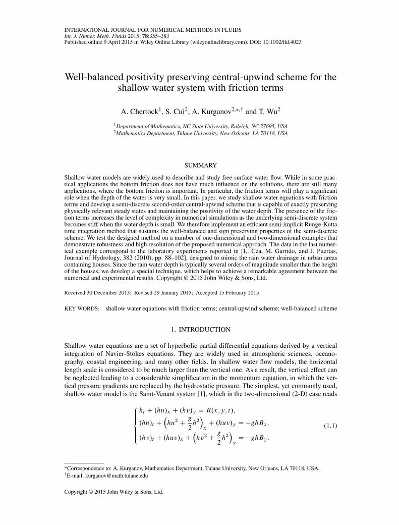
The system (1.2) still admits ‘lake at rest’ steady states. However, we are interested in simulatingdrainage of the rain water in urban areas. In such situations, the simplest yet physically relevantquasi one-dimensional (1-D) steady-state solutions correspond to the case when the water flows overa slanted infinitely long surface with a constant slope as illustrated in Figure 1 (left). Such steadystates (both 1-D and 2-D) are discussed in Section 2.
A well-balanced Roe-type numerical scheme that exactly preserves steady states shown inFigure 1 was proposed in [24]. However, to maintain the positivity of the water depth h, the schemein [24] requires one to use very small time steps and thus may not be robust in certain settings.Another Godunov-type scheme for the 1-D version of (1.2) was proposed in [25]. Though thismethod does not suffer from restrictive time stepping, it is capable of preserving ‘lake at rest’ steadystates only.
Figure 1. The bottom setting of numerical examples. The figure on the left corresponds to the quasi one-dimensional steady state. The figure on the right illustrates the case of urban draining with obstacles like
houses. The slope of the bottom and the height of the houses are out of scale.
In this paper, we develop a central-upwind scheme for the system (1.2), which is well-balanced,positivity preserving, and efficient. Central-upwind schemes have been proposed for general hyper-bolic system of conversation law in [26–29] and extended to the shallow water equations and relatedmodels in [8, 9, 30]. These schemes belong to the family of Godunov-type central schemes thatare Riemann-problem-solver-free, robust, and highly accurate. The extension of central-upwindschemes to the shallow water systems with friction terms is very natural and it is described in boththe 1-D (Section 3.1) and 2-D (Section 3.2) cases (the 2-D scheme presented here is restricted toCartesian meshes). The efficiency of the proposed central-upwind scheme hinges on the use of anefficient second-order semi-implicit ODE solver we have recently developed in [31] and brieflydescribe in Section 3.3.
The designed scheme is tested in a number of numerical experiments including those with realisticurban bottom topography structures, schematically shown in Figure 1 (right). The results presentedin Section 4 demonstrate the superb performance of the proposed numerical method. The data inExample 8 correspond to the laboratory experiments reported in [32], designed to mimic the rain-water drainage in urban areas containing houses. Since the rainwater depth is typically severalorders of magnitude smaller than the height of the houses, the proposed central-upwind schemehas been modified to accurately handle such situations as follows. First, the houses are removedfrom the computational domain, which becomes a punctured domain with many internal solid wallboundary pieces. Second, the rainwater falling over the houses is redistributed to the areas nearthe edges of the houses. This helps to achieve a remarkable agreement between the numerical andexperimental results.
2. STEADY-STATE SOLUTIONS
In this section, we discuss steady-state solutions of the shallow water system (1.2). We begin withthe simplest 1-D case, in which the system (1.2) reduces to8<:
ht C .hu/x D R.x; t/;
.hu/t C�hu2 C
g
2h2�xD �ghBx � g
n2
h1=3juju:
(2.1)
In the situation when the water source is zero (R � 0), the steady-state solution satisfies the time-independent system: 8<:
.hu/x D 0;�hu2 C
g
2h2�xD �ghBx � g
n2
h1=3juju:
(2.2)
In general, this system is not solvable, but one can obtain a particular nontrivial (u ¤ 0) steady statein the form
This solution corresponds to the situation when the water flows over a slanted infinitely long surfacewith a constant slope. Indeed, if we assume that Bx � �C , where C > 0 is a constant, and denotehu � q0, then the second equation of (2.2) can be rewritten as�
�q20h2C gh
�hx D ghC � g
n2
h1=3juju; (2.4)
and one obtains
h � h0 D
�n2q20C
�3=10; hu � q0; Bx � �C; (2.5)
where h0 is the so-called normal depth. A simple analysis of the ODE (2.4) shows that this steadystate is expected to be stable in the supercritical case, that is, when h0 is below the critical depth hc :
h0 < hc WD�q0g
�1=3: (2.6)
The structure of 2-D steady states is substantially more complicated. However, the quasi 1-D steady-state solutions
h � constant; hu � constant; hv � 0; Bx � constant; By � 0; (2.7)
or
h � constant; hu � 0; hv � constant; Bx � 0; By � constant (2.8)
are still physically relevant to the situation depicted in Figure 1.In the next sections, we design both 1-D and 2-D central-upwind schemes that exactly preserve
the aforementioned steady states (2.5) and (2.7), (2.8), respectively.
3. NUMERICAL METHOD
In this section, we present a well-balanced and positivity preserving semi-discrete central-upwindscheme for the shallow water equations with friction terms in both 1-D and 2-D. The scheme isderived along the lines of [9], and, therefore, here, we only describe its main components followingthe key ideas from [9]. In particular, the well-balanced property of the scheme will be ensured by aspecial finite-volume-type quadrature used for discretizing the geometric source term on the right-hand side of the system. We also introduce a new variable for the water surface w WD hC B . As ithas been shown in [9], working with w (rather than with h) is important for preserving ‘lake at rest’steady states at the discrete level. Even though in this work, we focus on different types of steadystates, described in Section 2, our goal is to design a numerical method, which preserves both the‘lake at rest’ and steady states (2.5), (2.7), and (2.8). The positivity preserving property is achievedby the following: (i) replacing the bottom topography function B with its continuous piecewiselinear (or bilinear in the 2-D case) approximation (done exactly the same way as in [9]); and (ii) aspecial positivity preserving correction of the piecewise linear reconstruction for the water surfacew (which is different from the one proposed in [9]).
It should be observed that a successful implementation of the central-upwind scheme wouldbe impossible without the use of an accurate and efficient time integration method that main-tains the aforementioned important features of the semi-discrete scheme. In what follows, we firstoverview the 1-D and 2-D central-upwind schemes in Sections 3.1 and 3.2, respectively, andthen, in Section 3.3, describe a new semi-implicit Runge-Kutta ODE solver we have recentlydeveloped in [31].
We start with a description of a well-balanced positivity preserving central-upwind scheme for the1-D shallow water equations (2.1). We first rewrite the system (2.1) in an equivalent form in termsof w WD hC B and q WD hu:8<:
wt C qx D R.x; t/;
qt C
�q2
w � BCg
2.w � B/2
�x
D �g.w � B/Bx � gn2
.w � B/7=3jqjq:
(3.1)
We use the notations
U WD
�w
q
�; F .U ; B/ WD
�q
q2
w�BC g
2.w � B/2
�and
S .U ; R;B/ WD
�R.x; t/
�g.w � B/Bx
�; M .U ; B/ WD
0
�g n2
.w�B/7=3jqjq
!;
so that the system of balance laws (3.1) takes the following vector form:
U t C F .U ; B/x D S .U ; R; B/CM .U ; B/: (3.2)
For simplicity, we introduce a uniform grid x˛ WD ˛�x, where �x is a small spatial scale andthe corresponding finite volume cells Cj WD Œxj� 12
; xjC 12�, and assume that at certain time level t ,
the solution is realized in terms of its cell averages, U j .t/ D 1�x
RCjU .x; t/ dx, which are evolved
in time according to the semi-discrete central-upwind scheme [8, 9, 27]:
d
dtU j .t/ D �
HjC 12.t/ �Hj� 12
.t/
�xC S j .t/CM j .t/ (3.3)
with the central-upwind numerical fluxes,Hj˙ 12, given by
HjC 12DaCjC 12
F .U�jC 12
; BjC 12/ � a�
jC 12F .UC
jC 12; BjC 12
/
aCjC 12� a�
jC 12
CaCjC 12
a�jC 12
aCjC 12� a�
jC 12
�UCjC 12� U�
jC 12
�:
(3.4)Note that all of the indexed quantities in (3.4) depend on time, but from now on, we suppress thetime-dependence of indexed quantities in order to shorten the notation.
In (3.4), U˙jC 12
are the right and left point values of the piecewise linear reconstruction
eUj .x/ D Uj C .Ux/j .x � xj /; 8x 2 Cj ; 8j; (3.5)
at x D xjC 12:
UCjC 12WD UjC1 �
�x
2.Ux/jC1; U�
jC 12WD Uj C
�x
2.Ux/j : (3.6)
To ensure the second-order accuracy and a non-oscillatory nature of the reconstruction, the numer-ical derivatives .Ux/j are to be computed using a nonlinear limiter, for example, the generalizedminmod limiters:
and the parameter � 2 Œ1; 2� controls the amount of numerical dissipation: The larger the � , thesmaller the numerical dissipation.
The use of a limiter does not, however, guarantee the positivity of h˙jC 12WD w˙
jC 12�BjC 12
, where
BjC 12WD
B�xjC 12
C 0�C B
�xjC 12
� 0�
2: (3.7)
Hence, to ensure the positivity of h˙jC 12
, we first replace the bottom topography function B.x/ with
its continuous piecewise linear approximation,
eB.x/ D Bj� 12 C .BjC 12 � Bj� 12 / � x � xj� 12�x; 8x 2 Cj ; 8j; (3.8)
for which the following property is satisfied:
Bj WD eB.xj / D 1
�x
ZCj
eB.x/ dx D BjC 12C Bj� 122
: (3.9)
Remark 3.1Notice that for the slanted bottom topography (Bx � constant), eB.x/ � B.x/. Also notice thatEquation (3.7) reduces to BjC 12
D B.xjC 12/ if B is continuous at x D xjC 12
.
Next, the reconstruction for w near (almost) dry areas has to be corrected because the use of (3.6)may lead to negative values of h˙
jC 12as it was shown in [9]. We therefore propose the following
correction procedure: In the cells, where the original reconstruction (3.6) produces negative valuesof h, we make the slope of h to be equal to the slope of B . Namely, we proceed as follows:
if w�jC 12
< BjC 12or wC
j� 12< Bj� 12
; then take .wx/j D .Bx/j
H) w�jC 12D hj C BjC 12
; wCj� 12D hj C Bj� 12
;
where hj WD wj � Bj . This correction (unlike the correction procedure in [9] or its more sophisti-cated modification recently proposed in [3]) not only will guarantee the positivity of h˙
jC 12but also
will be able to exactly reconstruct the steady-state solution (2.5).It should also be pointed out that when the solution is expected to have (almost) dry areas, say,
when the computational domain contains ‘islands’ and/or ‘coastal areas’, the values of h could bevery small or even zero. This may not allow us to (accurately) compute the values of the veloc-ity u, which may become artificially large. In such cases, when in some cells, the point valuesh˙j˙ 12
are smaller than an a priori chosen positive number ", that is, h˙j˙ 12
< ", the piecewise lin-
ear reconstruction of q in (3.5) should be replaced with a piecewise linear reconstruction of u inthe entire computational domain. Namely, the velocity at the cell centers is first computed by thedesingularization formula
uj D2 hj � qj
h2
j Cmax�h2
j ; "2� ; (3.10)
and then the point values of the velocity at the cell interfaces x D xjC 12are obtained from
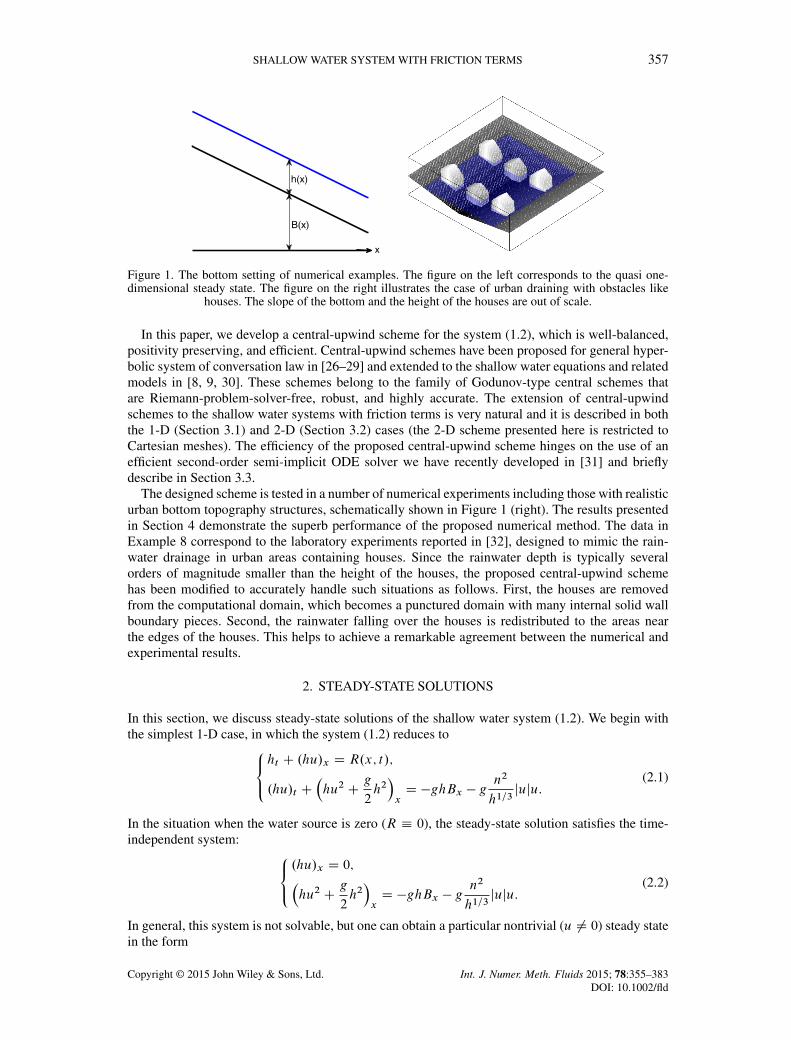
where the numerical derivative .ux/j are evaluated using the same nonlinear limiter as in (3.5). Forconsistency, the values of the discharge at cell interfaces are recomputed using q˙
j˙ 12D h˙
j˙ 12�u˙j˙ 12
.
Remark 3.2We note that one may use other strategies to compute the desingularized velocity:
u D
p2hqp
h4 Cmax .h4; "4/;
or
u D
´ qh; if h > ";
0; otherwise;
see, for example, the discussion in [9]. Our numerical experiments demonstrate that the proposedmethod is not sensitive to the selection of the desingularization procedure used.
Next, equipped with the values of h˙jC 12
and u˙jC 12
, we complete the construction of the central-
upwind flux (3.4) by estimating the one-sided local speeds of propagation as follows:
aCjC 12D max
²uCjC 12C
rghC
jC 12; u�
jC 12Cqgh�
jC 12; 0
³;
a�jC 12D min
²uCjC 12�
rghC
jC 12; u�
jC 12�qgh�
jC 12; 0
³:
(3.11)
The final step in the derivation of the semi-discrete scheme is the discretization of the sourceterms:
S j .t/ �1
�x
ZCj
S.U; R;B/ dx; M j .t/ �1
�x
ZCj
M .U; B/ dx:
We calculate the first component of S j using the midpoint rule:
S.1/
j D R.xj ; t /;
while approximate the geometric source in S.2/
j using a special quadrature derived in [8, 9], whichguarantees the well-balancedness of the resulting scheme:
S.2/
j D �ghjBjC 12
� Bj� 12�x
: (3.12)
The second component ofM j is computed using the desingularization procedure (3.10):
M.2/
j D �g n2
0@ 2 hj
h2
j Cmax�h2
j ; "2�1A7=3 jqj jqj : (3.13)
We remark that the semi-discrete scheme (3.3), (3.4) is a system of time-dependent ODEs, whichshould be solved using a high-order (at least second order accurate) and efficient method as wediscuss in Section 3.3 in the succeeding texts.
In this section, we describe the central-upwind scheme for the 2-D shallow water system (1.2). Asin the 1-D case, we rewrite the system (1.2) in terms of the new unknown vector U D .w; q WDhu; p WD hv/T :
U t C F .U ; B/x CG .U ; B/y D S .U ; R;B/CM .U ; B/; (3.14)
where the fluxes and the source terms are:
F .U ; B/ D
�q;
q2
w � BCg
2.w � B/2;
qp
w � B
�T;
G .U ; B/ D
�p;
qp
w � B;p2
w � BCg
2.w � B/2
�T;
S .U ; R; B/ D�R;�g.w � B/Bx ;�g.w � B/By
;
M .U ; B/ D
�0;�g
n2
h7=3qpq2 C p2;�g
n2
h7=3ppq2 C p2
�T:
We denote by Cj;k the computational cells Cj;k D Œxj� 12; xjC 12
� � Œyk� 12; ykC 12
�, where x˛ WD˛�x and yˇ WD ˇ�y, where �x and �y are small spatial scales, and write a central-upwindsemi-discretization of (3.14) as the system of ODEs:
d
dtU j;k D �
H x
jC 12 ;k�H x
j� 12 ;k
�x�Hy
j;kC 12�H
y
j;k� 12
�yC S j;k CM j;k; (3.15)
for the time evolution of the cell averages, U j;k.t/ D1
�x�y
’Cj;k
U .x; y; t/ dxdy. As in the 1-D
case, we follow [9, 29] and obtain the central-upwind numerical fluxes in the form
H x
jC 12 ;kDaCjC 12 ;k
F�UEj;k; BjC 12 ;k
�� a�
jC 12 ;kF�UWjC1;k; BjC 12 ;k
�aCjC 12 ;k
� a�jC 12 ;k
CaCjC 12 ;k
a�jC 12 ;k
aCjC 12 ;k
� a�jC 12 ;k
hUWjC1;k � U
Ej;k
i;
Hy
j;kC 12DbCj;kC 12
G�UNj;k; Bj;kC 12
�� b�
j;kC 12G�U Sj;kC1; Bj;kC 12
�bCj;kC 12
� b�j;kC 12
CbCj;kC 12
b�j;kC 12
bCj;kC 12
� b�j;kC 12
hU Sj;kC1 � U
Nj;k
i:
(3.16)
Here, Bj˙ 12 ;kand Bj;k˙ 12
are the values of the piecewise bilinear approximation of B:
eB.x; y/ D Bj� 12 ;k� 12 C �BjC 12 ;k� 12 � Bj� 12 ;k� 12 � � x � xj� 12�x
Remark 3.3For the slanted bottom topography satisfying either Bx � constant; By � 0 or Bx � 0; By �constant, the approximant (3.17) is exact, that is, eB.x; y/ � B.x; y/.
The values UE;W;N;Sj;k
in (3.16) are the point values of the piecewise linear reconstruction
eU .x; y/ D U j;k C .U x/j;k.x � xj /C .U y/j;k.y � yk/; .x; y/ 2 Cj;k; (3.19)
at .xjC 12; yk/, .xj� 12
; yk/, .xj ; ykC 12/, .xj ; yk� 12
/, respectively. Namely, we have
UEj;k WDeU �xjC 12 � 0; yk� D U j;k C �x
2.U x/j;k ;
UWj;k WDeU �xj� 12 C 0; yk� D U j;k � �x2 .U x/j;k ;
UNj;k WDeU �xj ; ykC 12 � 0� D U j;k C �y
2
�U y
j;k;
U Sj;k WDeU �xj ; yk� 12 C 0� D U j;k � �y2 �
U yj;k:
As in the 1-D case, the numerical derivatives .U x/j;k and .U y/j;k are to be computed using anonlinear limiter, say, the generalized minmod limiter (for details, see [9]).
To preserve the positivity of water height h, we follow the 1-D approach presented in Section 3.1and correct the reconstructed values of w as follows:
if wEj;k < BjC 12 ;kor wWj;k < Bj� 12 ;k
; then take .wx/j;k D .Bx/j;k
H) wEj;k D BjC 12 ;kC hj;k; wWj;k D Bj� 12 ;k
C hj;kI
if wNj;k < Bj;kC 12or wSj;k < Bj;k� 12
; then take .wy/j;k D .By/j;k
H) wNj;k D Bj;kC 12C hj;k; wSj;k D Bj;k� 12
C hj;k;
where hj;k WD wj;k � Bj;k .Once again, we observe that the obtained point values of h may be very small or even zero.
Similarly, to the 1-D case, when the solution contains (almost) dry areas, that is, if hjC 12 ;k< " or
hj;kC 12< " somewhere in the computational domain, we reconstruct the velocities u and v instead
of the discharges q and p. To this end, we first compute the velocities at the cell centers:
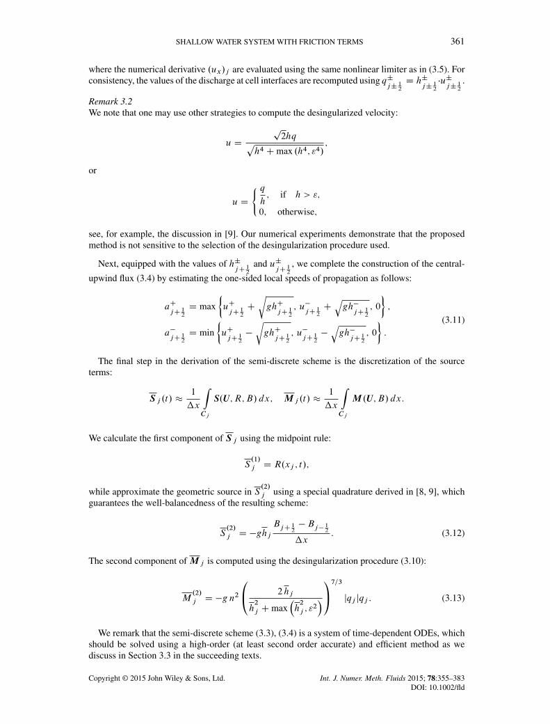
and evaluate the point values at the cell interfaces using the piecewise linear reconstructions:
uEj;k WD uj;k C
�x
2.ux/j;k; uW
j;k WD uj;k ��x
2.ux/j;k;
uNj;k WD uj;k C
�y
2.uy/j;k; uS
j;k WD uj;k ��y
2.uy/j;k
vEj;k WD vj;k C
�x
2.vx/j;k; vW
j;k W vj;k ��x
2.vx/j;k;
vNj;k WD vj;k C
�y
2.vy/j;k; vS
j;k WD vj;k ��y
2.vy/j;k;
where the numerical derivatives .ux/j;k ; .vx/j;k ; .uy/j;k , and .vy/j;k are computed with the helpof the same nonlinear limiter used in (3.19). The obtained values are then used to recompute thecorresponding point values of q and p:
qE(W,N,S)j;k
D hE(W,N,S)j;k
� uE(W,N,S)j;k
; pE(W,N,S)j;k
D hE(W,N,S)j;k
� vE(W,N,S)j;k
:
The local one-sided speeds of propagation a˙jC 12 ;k
and b˙j;kC 12
in (3.16) can be estimated as
follows:
aCjC 12 ;k
D max¹uEj;k CqghE
j;k; uWjC1;k C
qghW
jC1;k; 0º;
a�jC 12 ;k
D min¹uEj;k �qghE
j;k; uWjC1;k �
qghW
jC1;k; 0º;
bCj;kC 12
D max¹vNj;k CqghN
j:k; vSj;kC1 C
qghS
j;kC1; 0º;
b�j;kC 12
D min¹vNj;k �qghN
j:k; vSj;kC1 �
qghS
j;kC1; 0º:
(3.21)
Finally, a well-balanced discretization of the source term is obtained using the same desingular-ization process as in (3.20) and is thus given by
S.1/
j;kD R.xj ; yk; t /; M
.1/
j;kD 0;
S.2/
j;kD �ghj;k
BjC 12 ;k� Bj� 12 ;k
�x; M
.2/
j;kD �gn2
qq2j;k C p
2j;k
0@ 2 hj;k
h2
j;k Cmax�h2
j;k; "21A7=3qj;k;
S.3/
j;kD �ghj;k
Bj;kC 12� Bj;k� 12�y
; M.3/
j;kD �gn2
qq2j;k C p
2j;k
0@ 2 hj;k
h2
j;k Cmax�h2
j;k; "2�1A7=3pj;k :
As in the 1-D case, in order to obtain a fully discrete scheme, the system (3.15), (3.16) should beintegrated by a stable and efficient ODE solver of at least second order of accuracy. We discuss thedetails of time integration in the next section.
3.3. Time integration method
As it was outlined in the previous sections, both the 1-D and 2-D semi-discrete central-upwindschemes are the systems of time-dependent ODEs that should be solved by an accurate, stable,and efficient method. A family of explicit strong stability preserving Runge-Kutta methods (SSP-RK) has been widely used in numerical simulations of various shallow water systems, see, forexample, [33, 34]. The presence of the stiff friction term in both (3.3) and (3.15) can lead, however,to a great loss in accuracy and efficiency of the ODE solver. In shallow water applications thatincluded dry and/or almost dry areas, the explicit treatment of the friction terms imposes a severetime step restriction, which is several order of magnitude smaller than a typical time step used forthe corresponding friction-free version of the studied system.
An attractive alternative to explicit methods is implicit-explicit SSP Runge-Kutta solvers, whichtreat the stiff part of the underlying ODE system implicitly and thus typically have the stabilitydomains based on the nonstiff term only, see, for example, [35–40]. However, a straightforwardimplementation of these methods may break the discrete balance between the fluxes, geometricsource, and the friction terms maintained by the derived semi-discrete central-upwind scheme, andthe resulting fully discrete method will not be able to preserve the relevant steady states and thepositivity of the computed water depth.
To overcome this difficulty, we have recently developed a family of second-order semi-implicittime integration methods for systems of ODEs with stiff damping term [31]. In these methods, onlya portion of the stiff term is implicitly treated, and therefore, the evolution equation is very easy tosolve and implement compared to fully implicit or implicit-explicit methods. The important featureof the ODE solvers we introduced in [31] resides in the fact that they are capable of exactly preserv-ing the steady states as well as maintaining the sign of the computed solution under the time steprestriction determined by the nonstiff part of the system only. The new semi-implicit methods arebased on the modification of explicit SSP-RK methods and are proven to have a formal second orderof accuracy, A.˛/-stability and stiff decay. We now briefly describe the application of the second-order semi-implicit ODE solver from [31] to the ODE system (3.3), (3.4) (the implementation ofthe ODE solver to the system (3.15), (3.16) is similar, and we thus omit it for the sake of brevity).
We first introduce the grid function of the numerical solution U WD°U j
±. We then denote the
discretization of the sum of fluxes, geometric, and water source terms by
FhUijWD �
H jC 12�H j� 12
�xC S j ; (3.22)
and introduce the discrete friction coefficient
G.U j / WD �gn20@ 2 hj
h2
j Cmax�h2
j ; "2�1A7=3 jqj j; (3.23)
so that the discretization of the friction term (3.13) can be written asM.2/
j D G.U j / qj . Using thesenotations, the ODE system (3.3) can be rewritten as8<
:d
dtwj D F .1/ŒU �j ;
d
dtqj D F .2/ŒU �j C G.U j / qj :
(3.24)
We now implement the SI-RK3 method to the system (3.24) (the SI-RK3 method is a second-order semi-implicit Runge-Kutta method based on the third-order SSP-RK method; for details, see[31, Section 3]). The resulting fully discrete scheme can be written as
In the following theorem, we prove that the fully discrete scheme (3.25) is well-balanced.
Theorem 3.1The fully discrete central-upwind scheme (3.25) is well-balanced in the sense that it preservessteady-state solutions satisfying
h � h0 D
�n2q20C
�3=10; q � q0; Bx � �C; R � 0 (3.26)
as long as h0 > ", where " is a desingularization parameter used in (3.10).
ProofWe first note that for the steady states (3.26), the numerical derivatives of U are given by U x �.�C; 0/T , and the numerical flux reduces to
H jC 12D�q0;
q20h0Cg
2h20
�T:
Therefore, H jC 12�H j� 12
� 0. The sums of the components of the source terms are also equal tozero, that is,
S.1/
j CM.1/
j D 0C 0 D 0; S.2/
j CM.2/
j D gh0C � gn2
h7=30
jq0jq0 D 0: (3.27)
The second equation can be proven true when h0 > " according to the definition of h0. Then, usingthe notations (3.22) and (3.23), we obtain that (3.27) is equivalent to
F .1/ŒU �j D 0; F .2/ŒU �j C G.U j / qj D 0;
which after being substituted into (3.25) implies hnC1
j D hn
j D h0 and qnC1j D qnj D q0. Wetherefore have proved that the steady state (3.26) is preserved. �
Remark 3.4Notice that the 2-D version of Theorem 3.1 can be proved in a similar manner.
Remark 3.5In [31], we have proved that the time step restriction for the SI-RK3 method is determined by thenonstiff (explicitly treated) term only and no extra time restrictions due to the stiffness of the frictionterm is required. This implies that for the ODE system (3.24), arising from the central-upwind semi-discretization of the 1-D shallow water system, the size of the time step is to be calculated based onthe CFL condition, namely, we need to select
are the local propagation speeds defined in (3.11).
Remark 3.6We would like to emphasize that [9, Theorem 2.1] directly applies to the first stage of the SI-RK3
method (3.25), and hence, the time step restriction (3.28) guarantees the positivity of hI
j WD wIj �Bj
for all j provided hj .t/ > 0 for all j . The positivity of hII
j , hIII
j , and hj .t C �t/ will then beensured by the same theorem provided�t 6 .�t/I� and�t 6 .�t/II� , where .�t/I� and .�t/II� are
computed using (3.28) applied to the intermediate solutions UI
and UII
, respectively. To satisfyall of the aforementioned time step restrictions, we implement the following adaptive strategy:
(i) Given the solution U .t/, set �t WD �.�t/�, where � 2 .0; 1/ and .�t/� is given by (3.28);
(ii) Use �t to compute UI
by (3.25a);
(iii) Given the intermediate solution UI
, compute .�t/I� by (3.28);(iv) If .�t/I� < �t , set �t WD �.�t/I� and go back to Step (ii);
(v) Use �t to compute UII
by (3.25b);
(vi) Given the intermediate solution UII
, compute .�t/II� by (3.28);(vii) If .�t/II� < �t , set �t WD �.�t/II� and go back to Step (ii);
(viii) Use �t to compute UIII
and U .t C�t/ by (3.25c) and (3.25d), respectively.
In all of the numerical examples in the succeeding texts, we have used � D 0:9.In the 2-D case, we have implemented a similar adaptive strategy to ensure the positivity of h.
However, the basic CFL condition is more restrictive (see [9, Theorem 3.1]), and one has to choose
�t 6 .�t/� WD min
²�x
4a;�y
4b
³; a D max
j;k
²aCjC 12 ;k
;�a�jC 12 ;k
³; b D max
j;k
²bCj;kC 12
;�b�j;kC 12
³;
where a˙jC 12 ;k
and b˙j;kC 12
are the local propagation speeds defined in (3.21).
4. NUMERICAL EXAMPLES
In this section, we test the designed well-balanced positivity preserving central-upwind schemeon several 1-D and 2-D problems including the ones with the data originating from the recentlyperformed laboratory experiments reported in [32]. In all of the examples in the succeeding texts,the gravitation constant g D 9:8 (in Example 4, we use g D 9:81), the minmod parameter � D 1:3,and we select the desingularization parameter " D 10�8 (in Example 4, we use " D 10�4, 10�8,and 10�12).
4.1. One-dimensional examples
Example 1 – Steady flow over a slanted surface. We begin by illustrating the well-balanced propertyof the designed scheme, that is, we test the ability of the scheme to exactly preserve the steady-statesolution (2.5), which is schematically shown in Figure 1 (left). To this end, we consider the system(2.1) on the interval Œ0; 2:5� with R � 0 and subject to the constant initial data given by (2.5). Weintroduce a uniform grid with �x D 0:025 and set zero-order extrapolation boundary conditionsat both ends of the domain, that is, h0 D h1; hNC1 D hN . We run five sets of experiments withdifferent values of h0, q0, Bx , and n, shown in Table I, in which the first four are taken from [32].The solution is evolved until time t D 100. The right column of Table I clearly illustrates that ourscheme preserves the studied steady-state solutions within machine accuracy.
Example 2 – Small perturbation of steady flow over a slanted surface. In this example, we takethe same initial data from Example 1 but introduce a small perturbation to the initial water surface,namely,
h.x; 0/ D h0 C
²0:2h0; 1 6 x 6 1:25;0; otherwise;
q.x; 0/ � q0: (4.1)
We first consider a supercritical case (Test 2 in Table I) and present several time snapshots of thecomputed solution in Figure 2. As one can see, the perturbation first changes its shape and propa-gates to the right, eventually leaving the domain. At large times, the computed solution convergesto the steady state ( Figure 2 (right)).
We then proceed with a subcritical case (Test 4 in Table I) and again replace the initial data inExample 1 with (4.1). The evolution of the perturbed solution is shown in Figure 3. In this case, theshape of the propagating perturbation is different from the one in the supercritical case, but at largetimes, the computed solution still converges to the steady state.
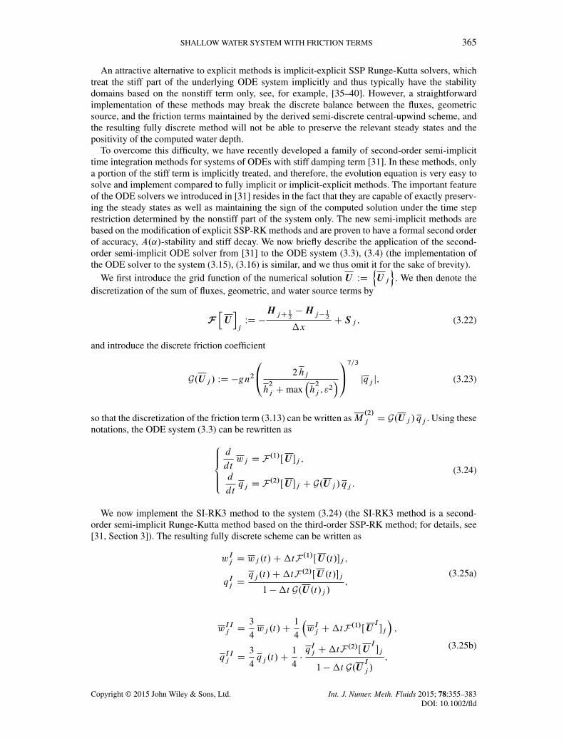
Finally, we consider Test 5 from Table I, in which the magnitude of the slope Bx is much largerthan in the other tests. In this case, the perturbation propagates much faster than in the previous twotests (Figure 4), but the scheme still performs very well and the numerical steady state is achievedat large times.
Example 3 – Rainfall-runoff over a slanted surface. In this example, which is a 1-D modificationof Example T3 from [24], we test the stability and accuracy of the proposed numerical scheme in
Table I. Example 1: Errors in computing the steady-state solution (2.5) fordifferent sets of data.
Test h0 q0 n Bx Froude number kh � h0k1
1 0.57708 2 0.02 �0.01 1.46 3:3307 � 10�16
2 0.09564 0.1 0.02 �0.01 1.08 5:8287 � 10�16
3 0.25119 0.1 0.1 �0.01 0.25 1:0547 � 10�15
4 0.02402 0.002 0.1 �0.01 0.17 1:8978 � 10�15
5 0.44894 2 0.1 �1=p3 2.12 4:9960 � 10�16
0 0.5 1 1.5 2 2.50.0
0.020.040.060.080.100.120.14
t=0
x
wB
0 0.5 1 1.5 2 2.50.0
0.020.040.060.080.100.120.14
t=1
x
wB
0 0.5 1 1.5 2 2.50.0
0.020.040.060.080.100.120.14
t=100
x
wB
Figure 2. Example 2: Evolution of the solution in the supercritical case (Test 2 in Table I).
0 0.5 1 1.5 2 2.5
0.01
0.02
0.03
0.04
0.05
0.06t=0
x
wB
0 0.5 1 1.5 2 2.5
0.01
0.02
0.03
0.04
0.05
0.06t=0.5
x
wB
0 0.5 1 1.5 2 2.5
0.01
0.02
0.03
0.04
0.05
0.06t=100
x
wB
Figure 3. Example 2: Evolution of the solution in the subcritical case (Test 4 in Table I).
the scenario with very shallow water, bed friction, and large bottom slope. The surface is assumedto be dry at time t D 0, that is, we set
h.x; 0/ � 0; q.x; 0/ � 0; (4.2)
and the bottom is set to be a slanted surface. The rain of a constant intensity starts falling at timet D 0 and stops at time t D 100. This is modeled by taking
R.x; t/ D
´10�4; 0 6 t 6 100;0; otherwise:
The water drains through the right boundary, at which we set
hNC1 WD 0; qNC1 WD 0;
where N is a total number of cells inside the computational domain Œ0; 2:5� (we take N D 100 inthis example). On the left side of the domain, we use solid wall boundary conditions.
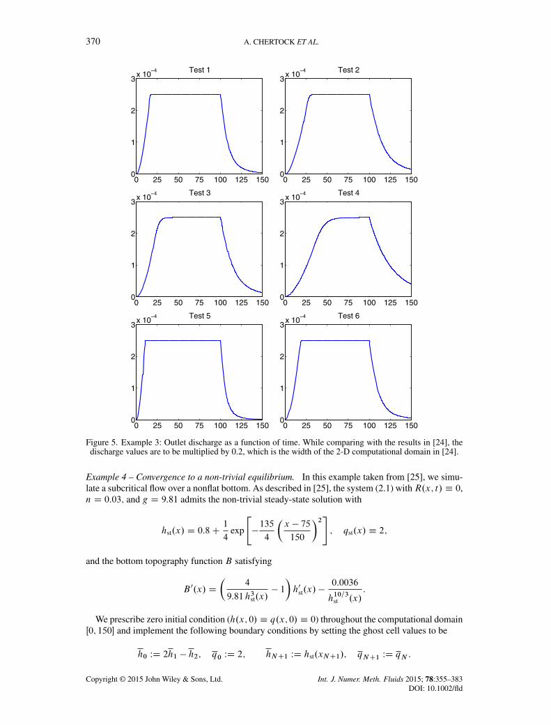
We consider six sets of data with different values of friction coefficient n and slope Bx (Table II)and run the simulations until time t D 150.
In Figure 5, we plot the first component of the numerical flux at the right edge of the compu-tational domain (H .1/
NC1=2) as a function of time. Notice that this is an approximation of the outlet
discharge, which is a measurable quantity in experimental settings. In all six cases, the resultsobtained by the designed central-upwind scheme are in a good agreement with the results reportedin [24]. We would like to point out that in [24], the simulations were performed in the 2-D domainof the width 0.2, so that all of the discharge values in Figure 5 are to be multiplied by the factor of0.2 in order to be compared with those in [24]. As one can clearly see from Figure 5, the reportedresults are oscillation-free confirming the robustness of the designed central-upwind scheme.
Remark 4.1It should be observed that if an upwind numerical scheme is used instead of the central-upwind one,the ghost cell values (4.2) may be unacceptable. We refer the reader to [24], where supercriticalboundary conditions have been implemented using a different ghost cell values:
hNC1 WD
q2Ng
!1=3; qNC1 WD qN :
In all of our computations, both types of boundary conditions produce similar results. However, thesupercritical boundary conditions sometime cause small oscillations.
Figure 5. Example 3: Outlet discharge as a function of time. While comparing with the results in [24], thedischarge values are to be multiplied by 0.2, which is the width of the 2-D computational domain in [24].
Example 4 – Convergence to a non-trivial equilibrium. In this example taken from [25], we simu-late a subcritical flow over a nonflat bottom. As described in [25], the system (2.1) withR.x; t/ � 0,n D 0:03; and g D 9:81 admits the non-trivial steady-state solution with
hst.x/ D 0:8C1
4exp
"�135
4
�x � 75
150
�2#; qst.x/ � 2;
and the bottom topography function B satisfying
B 0.x/ D
�4
9:81 h3st.x/� 1
�h0st.x/ �
0:0036
h10=3st .x/
:
We prescribe zero initial condition (h.x; 0/ � q.x; 0/ � 0) throughout the computational domainŒ0; 150� and implement the following boundary conditions by setting the ghost cell values to be
In addition, we fix the first component of inlet numerical flux by setting
H.1/12
WD 2
for all times.The solution of the studied initial-boundary value problem is expected to converge to the afore-
mentioned steady state as t !1. We test our scheme on different grids varying the number of cellsN from 50 to 1600 and study the convergence rate by comparing the computed solutions with thesteady-state one at time Tmax D 1200. The solution (w and q) computed with N D 50 is plotted inFigure 6 together with the steady-state solution. As one can see, the proposed method captures theexact steady state quite accurately even on such a coarse grid (the obtained results are a little bet-ter than the one reported in [25]). When the mesh is refined, the second-order convergence rate isobserved in h, while the q component converges with almost third order (Table III), where we showboth the L1-norm and L1-norm of the errors together with the experimental convergence rates.
Example 5 – Oscillating lake. We consider shallow water flow with wet/dry fronts in a frictionalparabolic bottom. This example is a modification of the numerical example studied in [41, 42]: Weuse the same initial data and bottom topography function, but we replace the linear friction termused in [41, 42] with the Manning friction term. The main goal of this example is to study the impactof the small parameter " in the desingularization procedure (3.10) on the computed solution.
We consider the bottom topography described by the function
B.x/ D 10
�� x
3000
�2� 1
�;
and set the following initial conditions:
w.x; 0/ D max¹k1x C k2; B.x/º; q.x; 0/ � 0;
where k1 D 0:0023660539018216433 and k2 D �1:25959748992322. We use the Manning frictionterm with the coefficient n D 0:02.
0 50 100 1500
0.5
1
1.5
2N=50Steady stateB
0 50 100 1501.99
1.995
2
2.005
2.01N=50Steady state
Figure 6. Example 4: Solution (w.x; 1200/ and q.x; 1200/) computed using N D 50 and the exact steady-state solution.
Table III. Example 4: The L1-error and L1-error and convergence rates for h and q.
h q
N L1-norm Rate L1-norm Rate L1-norm Rate L1-norm Rate
We run the simulation over the computation domain Œ�5000; 5000�, which is divided intoN D 1000 cells. We use three different values of the desingularization parameter " D 10�4, 10�8,and 10�12 and compute the solutions until the final time t D 3000. The snapshots of the com-puted solutions at t D 300, 1000, and 3000 are shown in Figure 7. As one can see, the solutionsobtained with the different values of " are almost indistinguishable. This clearly demonstrates thatthe proposed central-upwind scheme is not sensitive to the selection of ".
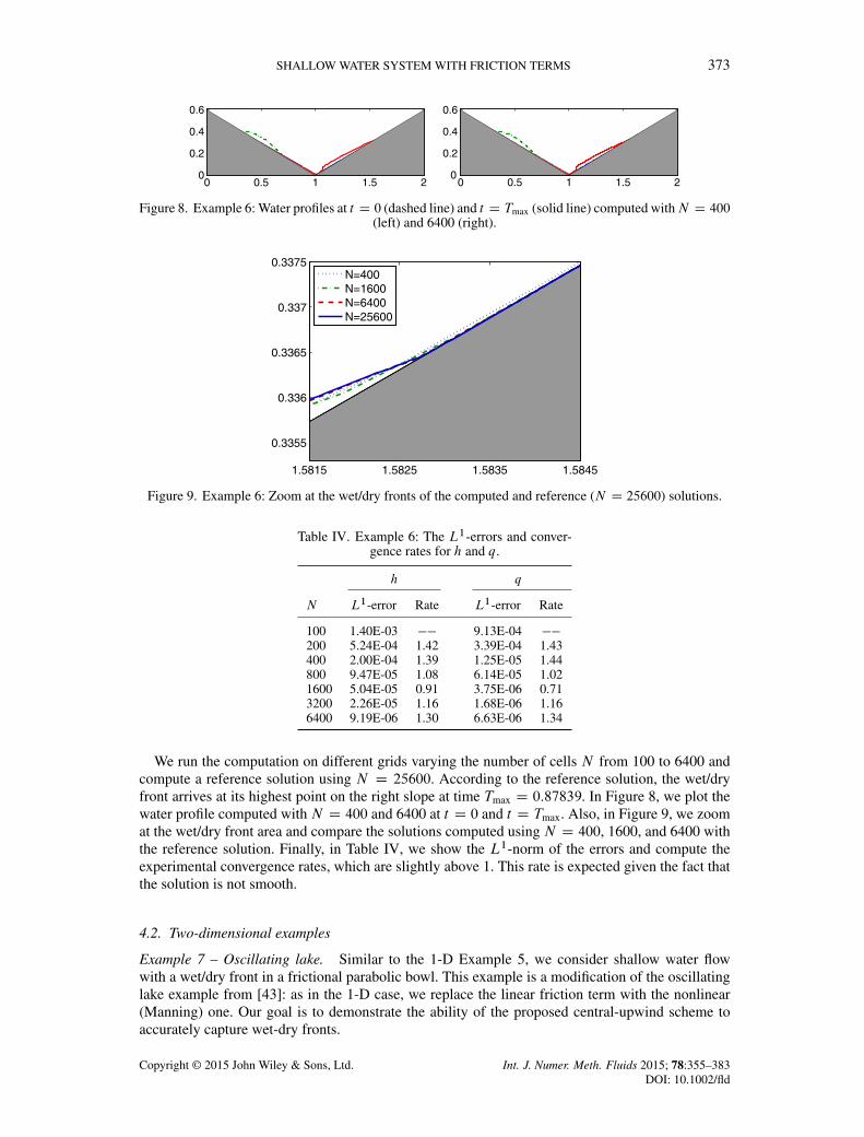
Example 6 – Wet/dry front propagation over a V-shape bottom topography. In this example, wesimulate a package of water released on the left part of a V-shape valley (Figure 8). The water steamsdown the left part and gradually accelerates. After passing the lowest point of the bottom, it startsclimbing up the right slope, meanwhile gradually losing its speed. Before the water starts streamingdown the right slope, the wet/dry front achieves its maximum height. Our goal is to study this frontpropagation quantitatively.
We consider a V-shape bottom topography function,
B.x/ D1p3jx � 1j;
and take the friction coefficient n D 0:02. Initially, a package of water has a parabolic profile andzero velocity:
h.x; 0/ D max ¹0;�1:5.x � 0:3/.x � 0:7/º ; q.x; 0/ � 0:
We take a computational domain to be sufficiently large (Œ0; 2�) so that the vibrating water bodynever reaches the boundaries.
−5000 0 5000−10
−5
0
5
10
15
20ε=10−4
ε=10−8
ε=10−12
B
−5000 0 5000−10
0
10
20
30
40
50ε=10−4
ε=10−8
ε=10−12
−5000 0 5000−1
0
1
2
3
4
5
ε=10−4
ε=10−8
ε=10−12
−5000 0 5000−10
−5
0
5
10
15
20ε=10−4
ε=10−8
ε=10−12
B
−5000 0 5000−30
−25
−20
−15
−10
−5
0
5ε=10−4
ε=10−8
ε=10−12
−5000 0 5000−4
−3
−2
−1
0
1ε=10−4
ε=10−8
ε=10−12
−5000 0 5000−10
−5
0
5
10
15
20ε=10−4
ε=10−8
ε=10−12
B
−5000 0 5000−5
0
5
10
15
20ε=10−4
ε=10−8
ε=10−12
−5000 0 5000−0.5
0
0.5
1
1.5
2
ε=10−4
ε=10−8
ε=10−12
Figure 7. Example 5: Snapshots of w, q, and u computed with " D 10�4, 10�8, and 10�12.
We run the computation on different grids varying the number of cells N from 100 to 6400 andcompute a reference solution using N D 25600. According to the reference solution, the wet/dryfront arrives at its highest point on the right slope at time Tmax D 0:87839. In Figure 8, we plot thewater profile computed with N D 400 and 6400 at t D 0 and t D Tmax. Also, in Figure 9, we zoomat the wet/dry front area and compare the solutions computed using N D 400, 1600, and 6400 withthe reference solution. Finally, in Table IV, we show the L1-norm of the errors and compute theexperimental convergence rates, which are slightly above 1. This rate is expected given the fact thatthe solution is not smooth.
4.2. Two-dimensional examples
Example 7 – Oscillating lake. Similar to the 1-D Example 5, we consider shallow water flowwith a wet/dry front in a frictional parabolic bowl. This example is a modification of the oscillatinglake example from [43]: as in the 1-D case, we replace the linear friction term with the nonlinear(Manning) one. Our goal is to demonstrate the ability of the proposed central-upwind scheme toaccurately capture wet-dry fronts.
where k1 D 0:002303379160180876 and k2 D 0:0005. We use the Manning friction term with thecoefficient n D 0:02.
We run the simulation until the final time Tmax D 100 in the computation domainŒ�5000; 5000�� Œ�5000; 5000�, which is divided intoN �N grid cells withN D 50, 100, 200, 400,and 800. The fine mesh (N D 800) solution is shown in Figure 10, where we show the computedwater surface (w), water depth (h), as well as the discharges (q and p), and velocities (u and v).As one can see, the wet/dry front is quite sharply captured by the central-upwind scheme, and thevelocities, which are computed using the desingularization procedure near the front, do not containlarge spikes, and thus, the efficiency of the scheme is maintained.
−4000 −2000 0 2000 4000
−4000
−2000
0
2000
4000
Figure 10. Example 7: Solution (w, h, q, u, p, and v) computed using the fine 800 � 800 grid.
To verify the rates of convergence of the proposed method, we measure the difference between thesolutions computed on two consecutive grids using the weighted L1-differences, which are definedas follows:
k�N � N k1 WD1
N 2
NXjD1
NXkD1
j�Nj;k � Nj;kj;
where �N WD ¹�Nj;kº and N WD ¹ N
j;kº are two functions prescribed on the N � N grid. To apply
this formula to the solutions computed on two different grids, we project the fine grid solution ontothe coarse grid using the conservative projection. Then, to measure the experimental convergencerates r for h, we use the ratio of the weighted L1-differences:
r D log2
khN=2 � hN=4k1
khN � hN=2k1
!:
The rates for q and p are computed similarly.The obtained results, reported in Table V, indicate that the experimental convergence rate of the
proposed central-upwind scheme is slightly smaller than 2.Example 8 – Rainfall runoff over an urban area. We consider another rainfall-runoff exam-
ple, which now occurs over a more complicated 2-D surface containing houses as outlined inFigure 1 (right).
The setting corresponds to the laboratory experiment reported in [32]. The surface structure isshown in Figure 11. The experimental setting was built to mimic an urban area within the labora-tory simulator of size 2 � 2:5meters. To model urban buildings, several blocks were placed ontothe surface according to different geometries, three of which are shown in Figure 11. In these threeconfigurations, the houses are aligned in either the x-direction (Configuration X20), y-direction(Configuration Y20), or both (Configuration S20). The bottom topography function B.x; y/ isdefined as
B.x; y/ D
².x; y/; outside the house region;H.x; yI xh; yh/; inside the house region centered at .xh; yh/:
Table V. Example 7: The weighted L1-differences between the solutions computed onconsecutive grids and the corresponding convergence rates.
Figure 11. Example 8: Three house configurations (X20 ,Y20, and S20) and contour plot of the urban areastructure S. In each configuration, the houses are placed in the blank rectangles such that the house ridges
The precise data of the surface structure S.x; y/ were provided by Dr. Luis Cea, and the house-roofconfiguration H.x; yI xh; yh/ was computed according to the following formulae:
H.x; yI xh; yh/ D²0:3 � jy � yhj; .x; y/ 2 Œxh � 0:15; xh C 0:15� � Œyh � 0:1; yh C 0:1�;0; otherwise;
0 25 50 75 100 125 150
1
2
3
4
5x 10⁻⁴
0 25 50 75 100 125 150
1
2
3
4
5x 10⁻⁴
0 25 50 75 100 125 150
1
2
3
4
5x 10⁻⁴
0 25 50 75 100 125 150
1
2
3
4
5x 10⁻⁴
0 25 50 75 100 125 150
1
2
3
4
5x 10⁻⁴
0 25 50 75 100 125 150
1
2
3
4
5x 10⁻⁴
0 25 50 75 100 125 150
1
2
3
4
5x 10⁻⁴
0 25 50 75 100 125 150
1
2
3
4
5x 10⁻⁴
0 25 50 75 100 125 150
1
2
3
4
5x 10⁻⁴
Figure 12. Example 8: Outlet discharge (the experimental data, dashed line, versus the computed results,solid line) as a function of time.
Figure 13. Example 8a: Special treatment of a house region. The house edges are considered to be a part ofan internal boundary. The rainfall on the roof is uniformly distributed into the shaded cells. There are two
cases: the one with the gutter system installed (left) and the one without such a system (right).
H.x; yI xh; yh/ D²0:3 � jx � xhj; .x; y/ 2 Œxh � 0:1; xh C 0:1� � Œyh � 0:15; yh C 0:15�;0; otherwise;
for houses aligned in y-direction. Notice that across the walls of the houses, the bottom topographyis discontinuous, and thus, the bilinear interpolant (3.17) has very sharp gradients there.
Similarly, to the 1-D rainfall-runoff example, we set the following almost dry initial conditions:
h.x; y; 0/ � 0; q.x; y; 0/ � 0; p.x; y; 0/ � 0:
Figure 14. Example 8a: Outlet discharge (the experimental data, solid line, versus the computed results,dashed line) as a function of time.
Figure 15. Example 8a: Outlet discharge as a function of time: convergence to a steady state when the rainsource is not switched off.
The rain of a constant intensity starts falling at time t D 0 and stops at t D Ts , that is,
R.x; y; t/ D
8<:1
12000; 0 6 t 6 Ts;
0; otherwise:
In different experiments, different values of Ts D 20, 40, 60, or 1 have been used. The compu-tational domain Œ�1; 1� � Œ0; 2:5� is divided into Nx � Ny uniform cells (we have taken Nx D 80
and Ny D 100). The solid wall boundary conditions have been set at the left, right, and top partsof the boundary, while absorbing boundary conditions have been implemented at the lower part(�1 6 x 6 1, y D 0). As in the 1-D case, we use the ghost cell technique, and the ghost cell valuesare set to be
At this boundary, the total outlet discharge is computed using �yNxXjD1
�Hy
j;1=2
.1/.
In Figure 12, the outlet discharge is plotted as a function of time and compared with theexperimental data provided to us by Dr. Luis Cea. Notice that in some cases (for example, for Con-figuration Y20 with Ts D 20 or 40 and Configuration S20), the computed curves have lower peaksthan the experimental ones. We believe that such a delay of outlet discharge can be explained byinability of the system (1.2)–(1.4) to accurately model the situation occurring near the house wallswhere the size of the jumps in the bottom topography is about 2-3 orders of magnitude larger thanthe water depth. We therefore modify the model by removing the houses from the computationaldomain and placing the entire rainwater, which would accumulate over the houses, near the housewalls inside the computational domain. The details of a modified approach are given in Example 8a.
Example 8a – Modified house treatment. We consider the same setting as in Example 8, butmake the following modifications.
First, we remove the houses from the computational domain, which becomes a punctured rectan-gle. A typical hole is depicted in Figure 13: The house walls become the internal boundary, which isnumerically treated using the solid wall ghost cell technique. Second, we redistribute the rainwaterfalling onto the roof so that it is placed inside the modified computational domain. In the laboratoryexperiment, the water falling on the house blocks streams down from the long (lower) edges andfinally joins the surface water flow, while in reality, the gutter system is commonly used and therainwater streams down from the rain pipes typically located at the house corners.
In the numerical experiments, we adopt two different strategies to mimic the aforementioned twodraining situations. In both cases, the building-roof rainfall is uniformly distributed on certain cells
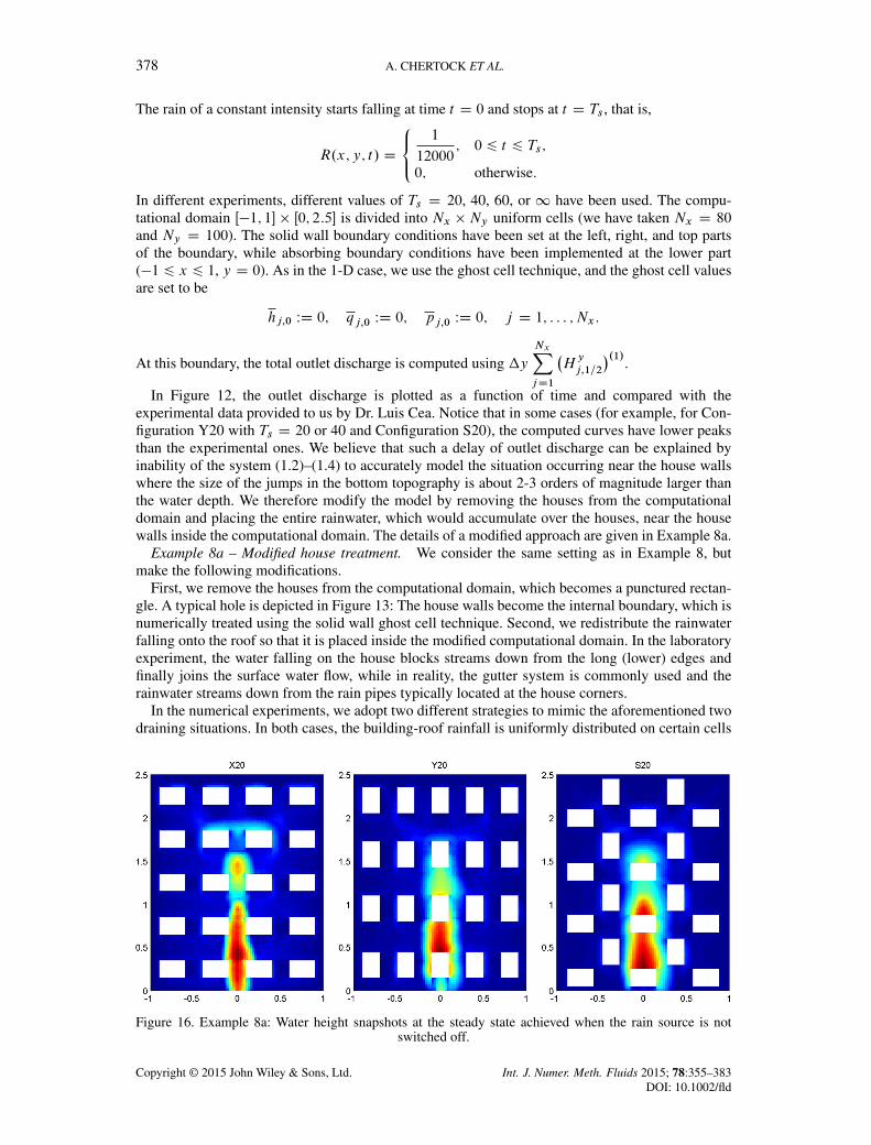
Figure 16. Example 8a: Water height snapshots at the steady state achieved when the rain source is notswitched off.
which is, as before, switched on only for t 2 Œ0; Ts�. Here, Ah is the area of the house, and As isthe area of the shaded region near that house. If the gutter system is installed, then in all studiedconfigurations (X20, Y20, and S20) with Nx D 80 and Ny D 100, we have
Ah
AsD0:2 � 0:3
4�x�yD 24:
If the gutter system is not installed, then this ratio depends on a house orientation, but since in thisnumerical example, we take �x D �y D 1=40, then
Ah
AsD
0:2 � 0:3
2 � 0:3�xD
0:2 � 0:3
2 � 0:3�yD 4
for all of the configurations (X20, Y20, and S20).Again, we compare the outlet discharges obtained by our numerical scheme and the laboratory
measurement. As we can see in Figure 14, our numerical results are now in much better agreementwith the experimental results, especially for Configurations Y20 (with Ts D 20 and 40) and S20. Inother cases, the achieved resolution is also slightly higher, though the improvement is not so essen-tial. It should also be observed that in the case of a longer rain duration (Ts D 60), the computedoutlet discharge remains almost constant for t 2 Œ30; 60� for Configurations X20 and Y20. In fact,if the rain source is not switched off (Ts D 1), the outlet discharge will converge to a steady stateas shown in Figure 15. The snapshots of a water height at this steady state are shown in Figure 16.
Finally, in Figure 17, we plot time snapshots of the water height obtained for Configurations X20,Y20, and S20 (we now use Ts D 40). The graphs illustrate how the rainwater drains and clarifythe dependence of the water flow on the surface configuration. In the examples using ConfigurationX20, the draining stream takes advantage of the space along the vertical central line x D 0 anda big mainstream is formed. In the examples using Configurations Y20 and S20, there are houseson the central line x D 0 that block the flow there. Therefore, the mainstream of draining waterhas to bypass these houses, and thus, small ‘lakes’ are developed behind two of the houses, seeConfigurations Y20 and S20 in Figure 17. This explains why the total amount of water flew out ofthe domain may not be the same as in the measured data because in the experimental setting, the‘lakes’ drain through the gaps between the building blocks and the bottom surface.
Remark 4.2We would like to point out that the aforementioned two different strategies of modifying therain source term near the houses lead to practically the same results. In the reported numerical
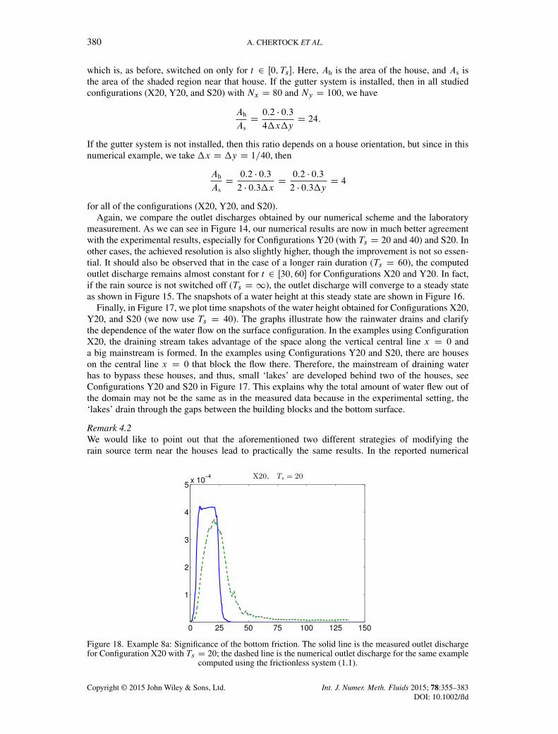
Figure 18. Example 8a: Significance of the bottom friction. The solid line is the measured outlet dischargefor Configuration X20 with Ts D 20; the dashed line is the numerical outlet discharge for the same example
experiments, we have redistributed the rain falling onto the house into the cells along the longerhouse edges (Figure 13, right) as discussed in the beginning of Example 8a.
Remark 4.3Another point, we would like to clarify the necessity of including the bottom friction terms in thestudied shallow water model. In Figure 18, we compare the measured data with the numerical resultobtained by solving the frictionless system (1.1). In this case, the computed outlet discharge changesdramatically even when the simplest Configuration X20 with Ts D 20 is considered.
5. CONCLUSION
We have studied the shallow water system with friction terms and developed a positivity preserv-ing semi-discrete central-upwind scheme, which is well-balanced in the sense that it is capable ofexactly preserving special types of steady-state solutions: both the ‘lake-at rest’ and ‘slanted surface’ones. Because of the presence of friction terms, the ODE system arising from the central-upwindsemi-discretization becomes stiff, and therefore, we have implemented an efficient semi-implicitRunge-Kutta time integration method that sustains the well-balanced and sign preserving propertiesof the semi-discrete scheme. We have tested the performance of the new method in a number of 1-Dand 2-D examples, including Example 8, which focuses on modeling the rainwater drainage in urbanareas that contain houses. Since the rainwater depth is typically several orders of magnitude smallerthan the height of the houses, a direct application of the shallow water equations leads to a sub-stantial discrepancy between the numerical and experimental results. We therefore have developed aspecial technique, according to which the houses are removed from the computational domain whilethe rainwater is redistributed into the nearby areas. The new technique helps to achieve a remarkableagreement between the numerical and experimental results.
ACKNOWLEDGMENT
The work of A. Chertock was supported in part by the NSF Grant DMS-1216974 and the ONRGrant N00014-12-1-0832. The work of A. Kurganov was supported in part by the NSF Grant DMS-1216957 and the ONR Grant N00014-12-1-0833. The work of S. Cui was supported in part by NSFGrants DMS-1115718 and DMS-1216957. The work of T. Wu was supported in part by the NSFGrants DMS-1115718 and DMS-1216957. A part of this research was conducted during the sum-mers of 2012 and 2013, when the authors visited the Institute of Natural Sciences at the ShanghaiJiao Tong University, China. The authors would like to thank the faculty, staff, and especially theInstitute co-director Prof. Shi Jin for their support and hospitality. The authors also thank Dr. MarioRicchiuto for encouraging discussions. The authors are thankful to Dr. Luis Cea for providing theexperimental data and for his help.
REFERENCES
1. de Saint-Venant AJC. Thèorie du mouvement non-permanent des eaux, avec application aux crues des rivière at àl’introduction des marèes dans leur lit. Comptes Rendus de L’Académie des Sciences 1871; 73:147–154.
2. Audusse E, Bouchut F, Bristeau M-O, Klein R, Perthame B. A fast and stable well-balanced scheme with hydrostaticreconstruction for shallow water flows. SIAM Journal on Scientific Computing 2004; 25:2050–2065.
3. Bollermann A, Chen G, Kurganov A, Noelle S. A well-balanced reconstruction for wet/dry fronts. Journal ofScientific Computing 2013; 56:267–290.
4. Bollermann A, Noelle S, Lukácová-Medvid’ová M. Finite volume evolution Galerkin methods for the shallow waterequations with dry beds. Communications in Computational Physics 2011; 10(2):371–404.
5. Bryson S, Epshteyn Y, Kurganov A, Petrova G. Well-balanced positivity preserving central-upwind scheme on tri-angular grids for the Saint-Venant system. ESAIM: Mathematical Modelling and Numerical Analysis 2011; 45(3):423–446.
6. Gallardo JM, Parés C, Castro M. On a well-balanced high-order finite volume scheme for shallow water equationswith topography and dry areas. Journal of Computational Physics 2007; 227(1):574–601.
7. Jin S, Wen X. Two interface-type numerical methods for computing hyperbolic systems with geometrical sourceterms having concentrations. SIAM Journal on Scientific Computing 2005; 26(6):2079–2101.
8. Kurganov A, Levy D. Central-upwind schemes for the saint-venant system. ESAIM: Mathematical Modelling andNumerical Analysis 2002; 36:397–425.
9. Kurganov A, Petrova G. A second-order well-balanced positivity preserving central-upwind scheme for the saint-venant system. Communications in Mathematical Sciences 2007; 5:133–160.
10. LeVeque RJ. Balancing source terms and flux gradients in high-resolution Godunov methods: the quasi-steady wave-propagation algorithm. Journal of Computational Physics 1998; 146(1):346–365.
11. Noelle Sebastian, Xing Yulong, Shu Chi-Wang. High-order well-balanced schemes, Numerical Methods for BalanceLaws, 2009; 1–66.
12. Perthame B, Simeoni C. A kinetic scheme for the Saint-Venant system with a source term. Calcolo 2001; 38(4):201–231.
13. Ricchiuto M, Bollermann A. Stabilized residual distribution for shallow water simulations. Journal of ComputationalPhysics 2009; 228(4):1071–1115.
14. Rogers B, Fujihara M, Borthwick A G L. Adaptive Q-tree Godunov-type scheme for shallow water equations.International Journal for Numerical Methods in Fluids 2001; 35(3):247–280.
15. Russo G, Khe A. High order well balanced schemes for systems of balance laws. In Hyperbolic Problems: Theory,Numerics and Applications, vol. 67, Proc. Sympos. Appl. Math. Amer. Math. Soc.: Providence, RI, 2009; 919–928.
16. Russo G, Khe A. High order well-balanced schemes based on numerical reconstruction of the equilibrium variables.Proceedings “WASCOM 2009” 15th Conference on Waves and Stability in Continuous Media, World Sci. Publ.,Hackensack, NJ, 2010; 230–241.
17. Xing Y, Shu C-W, Noelle S. On the advantage of well-balanced schemes for moving-water equilibria of the shallowwater equations. Journal of Scientific Computing 2011; 48(1–3):339–349.
18. Gerbeau J-F, Perthame B. Derivation of viscous Saint-Venant system for laminar shallow water; numerical validation.Discrete and Continuous Dynamical Systems - Series B 2001; 1(1):89–102.
19. Kellerhals R. Stable channels with gravel-paved beds. ASCE Journal of the Waterways and Harbors Division 1967;93(1):63–84.
20. Flamant A. Mécanique Appliquée : Hydraulique. Baudry éditeur: Paris, France, 1891.21. Darcy H. Recherches expérimentales Relatives au mouvement de l’eau dans les tuyaux, Vol. 1. Mallet-Bachelier:
Paris, 1857.22. Gauckler Ph. Etudes théoriques et pratiques sur l’ecoulement et le mouvement des eaux. Gauthier-Villars: Paris,
1867.23. Manning R. On the flow of water in open channel and pipes. Transactions of the Institution of Civil Engineers of
Ireland 1891; 20:161–207.24. Cea L, Vázquez-Cendón M E. Unstructured finite volume discretisation of bed friction and convective flux in solute
transport models linked to the shallow water equations. Journal of Computational Physics 2012; 231(8):3317–3339.25. Berthon C, Marche F, Turpault R. An efficient scheme on wet/dry transitions for shallow water equations with
friction. Computers & Fluids 2011; 48:192–201.26. Kurganov A, Lin C-T. On the reduction of numerical dissipation in central-upwind schemes. Communications in
Computational Physics 2007; 2:141–163.27. Kurganov A, Noelle S, Petrova G. Semi-discrete central-upwind scheme for hyperbolic conservation laws and
Hamilton-Jacobi equations. SIAM Journal on Scientific Computing 2001; 23:707–740.28. Kurganov A, Tadmor E. New high resolution central schemes for nonlinear conservation laws and convection-
diffusion equations. Journal of Computational Physics 2000; 160:241–282.29. Kurganov A, Tadmor E. Solution of two-dimensional Riemann problems for gas dynamics without Riemann problem
solvers. Numerical Methods for Partial Differential Equations 2002; 18:584–608.30. Kurganov A, Petrova G. Central-upwind schemes for two-layer shallow equations. SIAM Journal on Scientific
Computing 2009; 31:1742–1773.31. Chertock A, Cui S, Kurganov A, Tong W. Steady state and sign preserving semi-implicit Runge-Kutta methods for
ODEs with stiff damping term. Submitted.32. Cea L, Garrido M, Puertas J. Experimental validation of two-dimensional depth-averaged models for forecasting
rainfall–runoff from precipitation data in urban areas. Journal of Hydrology 2010; 382:88–102.33. Gottlieb S, Ketcheson D, Shu C.-W. Strong Stability Preserving Runge-Kutta and Multistep Time Discretizations.
World Scientific Publishing Co. Pte. Ltd.: Hackensack, NJ, 2011.34. Gottlieb S, Shu C.-W., Tadmor E. Strong stability-preserving high-order time discretization methods. SIAM Review
equations. Applied Numerical Mathematics 1997; 25(2–3):151–167. Special issue on time integration (Amsterdam,1996).
36. Higueras I, Roldán T. Positivity-preserving and entropy-decaying IMEX methods. In Ninth International ConferenceZaragoza-Pau on Applied Mathematics and Statistics, vol. 33, Monogr. Semin. Mat. García Galdeano. Prensas Univ.Zaragoza: Zaragoza, 2006; 129–136.
37. Hundsdorfer W, Ruuth S J. IMEX extensions of linear multistep methods with general monotonicity and boundednessproperties. Journal of Computational Physics 2007; 225(2):2016–2042.
38. Higueras I, Happenhofer N, Koch O, Kupka F. Optimized strong stability preserving IMEX Runge–Kutta methods.Journal of Computational and Applied Mathematics 2014; 272:116–140.
39. Pareschi L, Russo G. Implicit-Explicit Runge-Kutta schemes and applications to hyperbolic systems with relaxation.Journal of Scientific Computing 2005; 25:129–155.
40. Pareschi L, Russo G. Implicit-explicit Runge-Kutta schemes for stiff systems of differential equations. In RecentTrends in Numerical Analysis, vol. 3, Adv. Theory Comput. Math. Nova Sci. Publ.: Huntington, NY, 2001; 269–288.
41. Sampson J, Easton A, Singh M. Moving boundary shallow water flow above parabolic bottom topography. TheANZIAM Journal 2005; 47((C)):C373–C387.
42. Sampson J, Easton A, Singh M. Moving boundary shallow water flow in a region with quadratic bathymetry. TheANZIAM Journal 2007/08; 49((C)):C666–C680.
43. Hou J, Liang Q, Simons F, Hinkelmann R. A stable 2D unstructured shallow flow model for simulations of wettingand drying over rough terrains. Computers & Fluids 2013; 82:132–147.