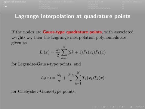
Spectral methods Well-conditioned collocation New TSEM Further studies Well-Conditioned Collocation Schemes and New Triangular Spectral-Element Methods Michael Daniel V. Samson [email protected]supervised by Li-Lian Wang Nanyang Technological University 29 April 2014
Transcript
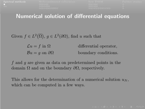
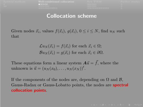
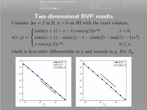
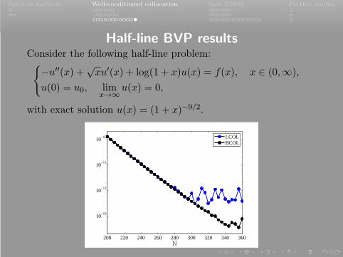
Spectral methods Well-conditioned collocation New TSEM Further studies
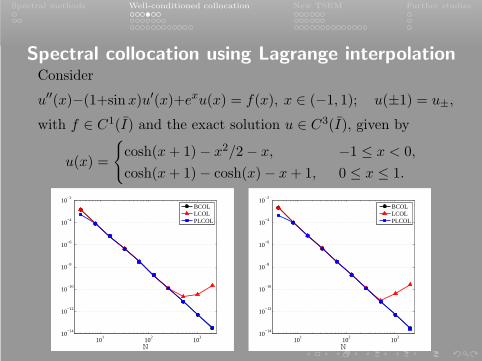
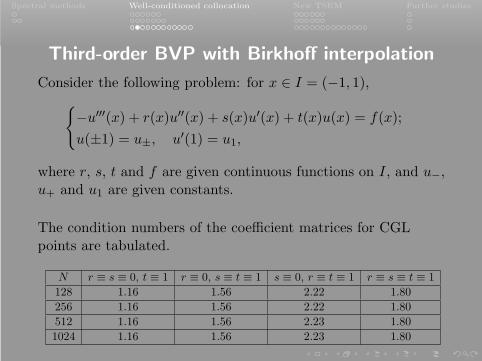
where r, s, t and f are given continuous functions on I, and u−,u+ and u1 are given constants.
The condition numbers of the coefficient matrices for CGLpoints are tabulated.
N r ≡ s ≡ 0, t ≡ 1 r ≡ 0, s ≡ t ≡ 1 s ≡ 0, r ≡ t ≡ 1 r ≡ s ≡ t ≡ 1
128 1.16 1.56 2.22 1.80
256 1.16 1.56 2.22 1.80
512 1.16 1.56 2.23 1.80
1024 1.16 1.56 2.23 1.80
Spectral methods Well-conditioned collocation New TSEM Further studies
Third-order Korteweg-de VriesConsider the third-order Korteweg-de Vries (KdV) equation:
∂tu+ u∂xu+ ∂3xu = 0, x ∈ (−∞,∞), t > 0; u(x, 0) = u0(x),
with the exact soliton solution
u(x, t) = 12κ2sech2(κ(x− 4κ2t− x0)),
where κ and x0 are constants. Let τ be the time step size. Usethe Crank-Nicolson leap-frog scheme in time and the newcollocation method in space: find uk+1
N ∈ PN+1 such that for0 < j < N ,
uk+1N (Lxj)− uk−1
N (Lxj)
2τ+ ∂3x
(uk+1N + uk−1
N
2
)(Lxj)
=− ∂xukN (Lxj)u
kN (Lxj);
ukN (±L) = ∂xukN (L) = 0, k ≥ 0.
Spectral methods Well-conditioned collocation New TSEM Further studies
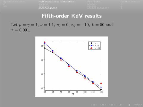
Third-order KdV results
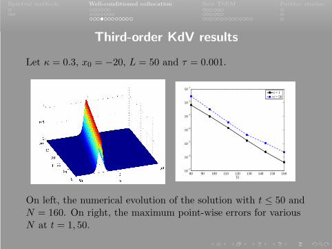
Let κ = 0.3, x0 = −20, L = 50 and τ = 0.001.
80 90 100 110 120 130 140 150 16010
−7
10−6
10−5
10−4
10−3
10−2
10−1
N
t = 1t = 50
On left, the numerical evolution of the solution with t ≤ 50 andN = 160. On right, the maximum point-wise errors for variousN at t = 1, 50.
Spectral methods Well-conditioned collocation New TSEM Further studies
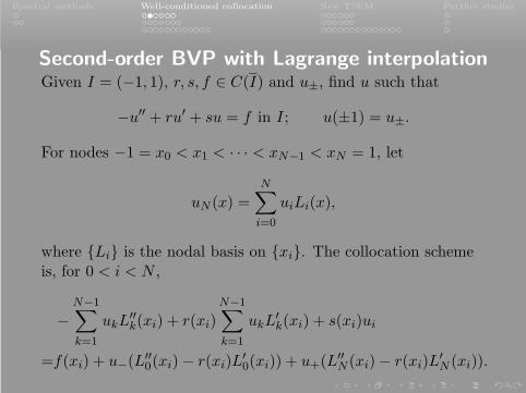
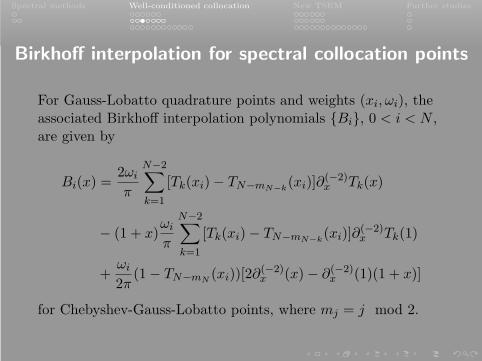
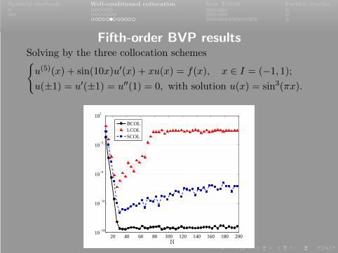
Fifth-order BVP with Birkhoff interpolationConsider the fifth-order problem:u(5)(x) + a(x)u′(x) + b(x)u(x) = f(x), x ∈ I = (−1, 1);
u(±1) = u′(±1) = u′′(1) = 0,
where a, b and f are given continuous functions on I.
Compare the generalized Lagrange interpolation p ∈ PN+3
satisfying, for u ∈ C5(I), u(±1) = u′(±1) = u′′(1) = 0,
Spectral methods Well-conditioned collocation New TSEM Further studies
Fifth-order Korteweg-de VriesConsider the fifth-order Korteweg-de Vries (KdV) equation:
∂tu+γu∂xu+ν∂3xu−µ∂5xu = 0, x ∈ (−∞,∞), t > 0; u(x, 0) = u0(x),
with the exact soliton solution
u(x, t) = η0+105ν2
169µγsech4
(√ν
52µ
[x−
(γη0 +
36ν2
169µ
)t− x0
]),
where γ, ν, µ, η0 and x0 are constants. Let τ be the time stepsize and ζj = Lxj . Use the Crank-Nicolson leap-frog scheme intime and the new collocation method in space: finduk+1N ∈ PN+3 such that for 0 < j < N ,
uk+1N (ζj)− uk−1
N (ζj)
2τ+ ν∂3x
(uk+1N + uk−1
N
2
)(ζj)− µ∂5x
(uk+1N + uk−1
N
2
)(ζj)
=− γ∂xukN (ζj)u
kN (ζj);
ukN (±L) = ∂xukN (±L) = ∂2xu
kN (L) = 0, k ≥ 0.
Spectral methods Well-conditioned collocation New TSEM Further studies
Selecting the test functions v to form a basis for T gives rise toa linear system.
Often, for spectral methods, Ω = (−1, 1)d, and T ⊂ PdN , the
space of tensorial polynomials of degree N in each component.Data gives interpolations IIN f ∈ Pd
N and IN g ∈ Pd−1N .
Spectral methods Well-conditioned collocation New TSEM Further studies
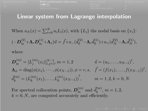
Linear system of variational formulationIf ψi, 0 ≤ i ≤ K, is a basis for u ∈ Pd
N , u = 0 on ∂ΩD, anduN (x) =
∑Ki=0 uiψi(x), for v = ψi, the discretized weak or
spectral-Galerkin formulation gives
BN (uN , ψi) =K∑
k=0
uk[(∇ψk,∇ψi)Ω + γ (ψk, ψi)Ω]
= (IIN f, ψi)Ω + 〈IN g, ψi〉N,∂ΩN= GN (ψi),
where the trace inner product is given by d− 1-dimensionalquadrature. The K + 1 equations gives the linear system
(S + γM)~u = ~f,
where S and M are the stiffness and mass matrices, resp.,
S = [(∇ψi,∇ψj)Ω]Ki,j=0, ~u = (u0, . . . , uK)t,
M = [(ψi, ψj)Ω]Ki,j=0,
~f = (GN (ψ0), . . . ,GN (ψK))t.
Spectral methods Well-conditioned collocation New TSEM Further studies
Spectral element method
Spectral element methods solve differential equations oversubdomains piecewise, in conjunction with some domain
decomposition method.
Spectral methods Well-conditioned collocation New TSEM Further studies
Spectral element method
Spectral element methods solve differential equations oversubdomains piecewise, in conjunction with some domaindecomposition method.
As in the finite-element method, let the domain Ω be asimplex.
Consider first the reference triangle
= (x, y), 0 < x, y, x+ y < 1
on the xy-plane. Herein, consider maps from the reference
square = (−1, 1)2 on the ξη-plane to , with the plan oftransforming the domain to to perform the operations.
Spectral methods Well-conditioned collocation New TSEM Further studies
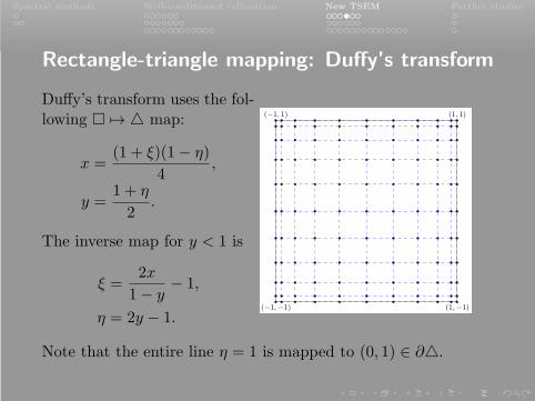
Rectangle-triangle mapping: Duffy’s transform
Duffy’s transform uses the fol-lowing 7→ map:
x =(1 + ξ)(1− η)
4,
y =1 + η
2.
The inverse map for y < 1 is
ξ =2x
1− y− 1,
η = 2y − 1.(−1,−1) (1,−1)
(1, 1)(−1, 1)
Note that the entire line η = 1 is mapped to (0, 1) ∈ ∂.
Spectral methods Well-conditioned collocation New TSEM Further studies
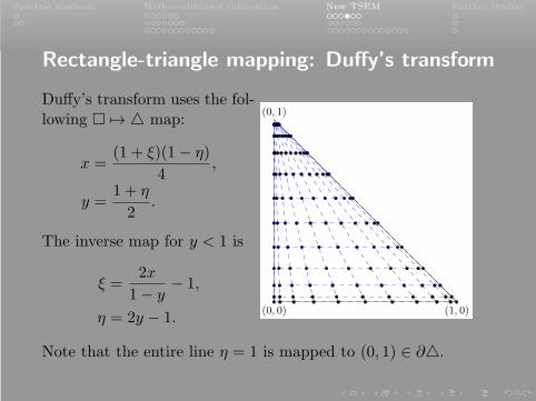
Rectangle-triangle mapping: Duffy’s transform
Duffy’s transform uses the fol-lowing 7→ map:
x =(1 + ξ)(1− η)
4,
y =1 + η
2.
The inverse map for y < 1 is
ξ =2x
1− y− 1,
η = 2y − 1.(0, 0) (1, 0)
(0, 1)
Note that the entire line η = 1 is mapped to (0, 1) ∈ ∂.
Spectral methods Well-conditioned collocation New TSEM Further studies
Transformed gradient for Duffy’s transform
Using the → map, given u(x, y) ∈ H1(), determineu(ξ, η) = u(x, y).
For Duffy’s transform, the Jacobian is
J =1− η
8,
and the gradient on is transformed on to
∇u =2
1− η
(2∂ξu, (1 + ξ)∂ξu+ (1− η)∂ηu
),
which requires the consistency condition ∂ξu(ξ, 1) = 0 to bebuilt into the approximation space to obtain high-orderaccuracy, resulting in the reduction of dimension andmodification of the usual basis functions.
Spectral methods Well-conditioned collocation New TSEM Further studies
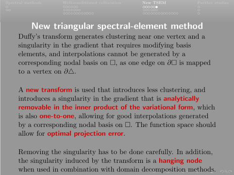
New triangular spectral-element methodDuffy’s transform generates clustering near one vertex and asingularity in the gradient that requires modifying basiselements, and interpolations cannot be generated by acorresponding nodal basis on , as one edge on ∂ is mappedto a vertex on ∂.
Spectral methods Well-conditioned collocation New TSEM Further studies
New triangular spectral-element methodDuffy’s transform generates clustering near one vertex and asingularity in the gradient that requires modifying basiselements, and interpolations cannot be generated by acorresponding nodal basis on , as one edge on ∂ is mappedto a vertex on ∂.
A new transform is used that introduces less clustering, andintroduces a singularity in the gradient that is analyticallyremovable in the inner product of the variational form, whichis also one-to-one, allowing for good interpolations generatedby a corresponding nodal basis on . The function space shouldallow for optimal projection error.
Removing the singularity has to be done carefully. In addition,the singularity induced by the transform is a hanging node
when used in combination with domain decomposition methods.
Spectral methods Well-conditioned collocation New TSEM Further studies
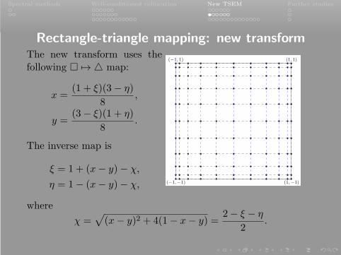
Rectangle-triangle mapping: new transformThe new transform uses thefollowing 7→ map:
x =(1 + ξ)(3− η)
8,
y =(3− ξ)(1 + η)
8.
The inverse map is
ξ = 1 + (x− y)− χ,
η = 1− (x− y)− χ, (−1,−1) (1,−1)
(1, 1)(−1, 1)
where
χ =√(x− y)2 + 4(1− x− y) =
2− ξ − η
2.
Spectral methods Well-conditioned collocation New TSEM Further studies
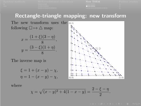
Rectangle-triangle mapping: new transformThe new transform uses thefollowing 7→ map:
x =(1 + ξ)(3− η)
8,
y =(3− ξ)(1 + η)
8.
The inverse map is
ξ = 1 + (x− y)− χ,
η = 1− (x− y)− χ, (0, 0) (1, 0)
(0, 1)
( 1
2,
1
2)
where
χ =√(x− y)2 + 4(1− x− y) =
2− ξ − η
2.
Spectral methods Well-conditioned collocation New TSEM Further studies
Transformed gradientUsing the → map, given u(x, y) ∈ H1(), determineu(ξ, η) = u(x, y).
For the new transform, the Jacobian is
J =2− ξ − η
16=χ
8,
and the gradient on is transformed on to
∇u =1
χ
(2(∇ · u) + ∇⊺u, 2(∇ · u)− ∇⊺u
),
where
∇u = (∂ξu, ∂ηu) and ∇⊺u = (1− ξ)∂ξu− (1− η)∂ηu.
Originally, the consistency condition ∇ · u(1, 1) = 0 was builtinto the approximation space. This singularity can be
removed, however; observe that∫∫
χ−1 dξ dη = 8 ln 2.
Spectral methods Well-conditioned collocation New TSEM Further studies
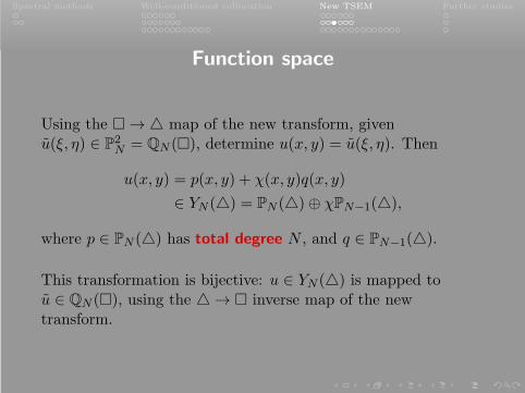
Function space
Using the → map of the new transform, givenu(ξ, η) ∈ P2
N = QN (), determine u(x, y) = u(ξ, η). Then
u(x, y) = p(x, y) + χ(x, y)q(x, y)
∈ YN () = PN ()⊕ χPN−1(),
where p ∈ PN () has total degree N , and q ∈ PN−1().
This transformation is bijective: u ∈ YN () is mapped tou ∈ QN (), using the → inverse map of the newtransform.
Spectral methods Well-conditioned collocation New TSEM Further studies
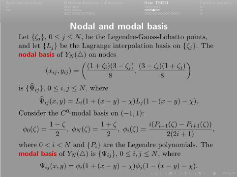
Nodal and modal basisLet ζj, 0 ≤ j ≤ N , be the Legendre-Gauss-Lobatto points,and let Lj be the Lagrange interpolation basis on ζj. Thenodal basis of YN () on nodes
(xij , yij) =
((1 + ζi)(3− ζj)
8,(3− ζi)(1 + ζj)
8
)
is Ψij, 0 ≤ i, j ≤ N , where
Ψij(x, y) = Li(1 + (x− y)− χ)Lj(1− (x− y)− χ).
Consider the C0-modal basis on (−1, 1):
φ0(ζ) =1− ζ
2, φN (ζ) =
1 + ζ
2, φi(ζ) =
i(Pi−1(ζ)− Pi+1(ζ))
2(2i+ 1),
where 0 < i < N and Pi are the Legendre polynomials. Themodal basis of YN () is Ψij, 0 ≤ i, j ≤ N , where
Ψij(x, y) = φi(1 + (x− y)− χ)φj(1− (x− y)− χ).
Spectral methods Well-conditioned collocation New TSEM Further studies
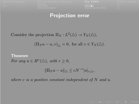
Projection error
Consider the projection ΠN : L2() → YN (),
(ΠNu− u, v) = 0, for all v ∈ YN ().
Theorem
For any u ∈ Hr(), with r ≥ 0,
‖ΠNu− u‖ ≤ cN−r|u|r,,
where c is a positive constant independent of N and u.
Spectral methods Well-conditioned collocation New TSEM Further studies
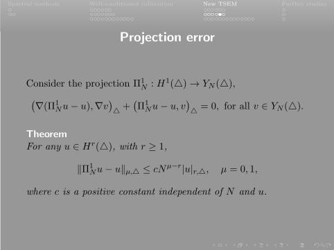
Projection error
Consider the projection Π1N : H1() → YN (),
(∇(Π1
Nu− u),∇v) +
(Π1
Nu− u, v) = 0, for all v ∈ YN ().
Theorem
For any u ∈ Hr(), with r ≥ 1,
‖Π1Nu− u‖µ, ≤ cNµ−r|u|r,, µ = 0, 1,
where c is a positive constant independent of N and u.
Spectral methods Well-conditioned collocation New TSEM Further studies
Projection error
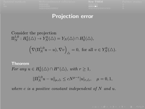
Consider the projectionΠ1,0
N : H10 () → Y 0
N () = YN () ∩H10 (),
(∇(Π1,0
N u− u),∇v)
= 0, for all v ∈ Y 0N ().
Theorem
For any u ∈ H10 () ∩Hr(), with r ≥ 1,
‖Π1,0N u− u‖µ, ≤ cNµ−r|u|r,, µ = 0, 1,
where c is a positive constant independent of N and u.
Spectral methods Well-conditioned collocation New TSEM Further studies
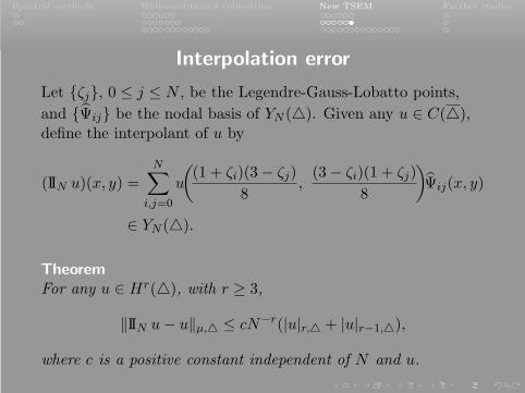
Interpolation error
Let ζj, 0 ≤ j ≤ N , be the Legendre-Gauss-Lobatto points,
and Ψij be the nodal basis of YN (). Given any u ∈ C(),define the interpolant of u by
(IIN u)(x, y) =N∑
i,j=0
u
((1 + ζi)(3− ζj)
8,(3− ζi)(1 + ζj)
8
)Ψij(x, y)
∈ YN ().
Theorem
For any u ∈ Hr(), with r ≥ 3,
‖IIN u− u‖µ, ≤ cN−r(|u|r, + |u|r−1,),
where c is a positive constant independent of N and u.
Spectral methods Well-conditioned collocation New TSEM Further studies
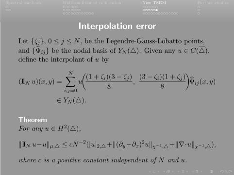
Interpolation error
Let ζj, 0 ≤ j ≤ N , be the Legendre-Gauss-Lobatto points,
and Ψij be the nodal basis of YN (). Given any u ∈ C(),define the interpolant of u by
where c is a positive constant independent of N and u.
Spectral methods Well-conditioned collocation New TSEM Further studies
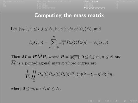
Computing the mass matrix
Let ψij, 0 ≤ i, j ≤ N , be a basis of YN (), and
φij(ξ, η) =N∑
m,n=0
pmnij Pm(ξ)Pn(η) = ψij(x, y).
Then M = P′MP , where P = [pmn
ij ], 0 ≤ i, j,m, n ≤ N and
M is a pentadiagonal matrix whose entries are
1
16
∫∫
Pm(ξ)Pm′(ξ)Pn(η)Pn′(η)(2− ξ − η) dξ dη,
where 0 ≤ m,n,m′, n′ ≤ N .
Spectral methods Well-conditioned collocation New TSEM Further studies
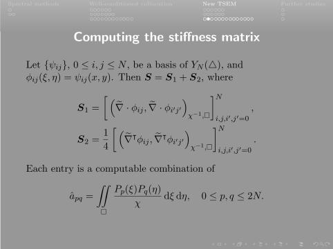
Computing the stiffness matrix
Let ψij, 0 ≤ i, j ≤ N , be a basis of YN (), andφij(ξ, η) = ψij(x, y). Then S = S1 + S2, where
S1 =
[(∇ · φij , ∇ · φi′j′
)χ−1,
]N
i,j,i′,j′=0
,
S2 =1
4
[(∇⊺φij , ∇⊺φi′j′
)χ−1,
]N
i,j,i′,j′=0
.
Each entry is a computable combination of
apq =
∫∫
Pp(ξ)Pq(η)
χdξ dη, 0 ≤ p, q ≤ 2N.
Spectral methods Well-conditioned collocation New TSEM Further studies
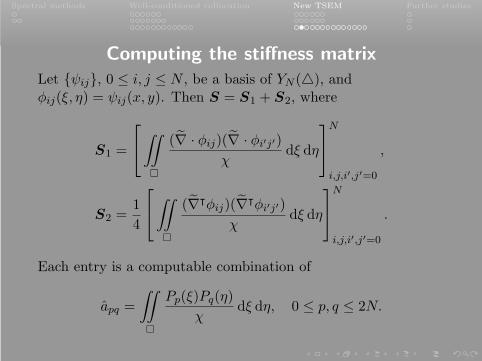
Computing the stiffness matrix
Let ψij, 0 ≤ i, j ≤ N , be a basis of YN (), andφij(ξ, η) = ψij(x, y). Then S = S1 + S2, where
S1 =
∫∫
(∇ · φij)(∇ · φi′j′)χ
dξ dη
N
i,j,i′,j′=0
,
S2 =1
4
∫∫
(∇⊺φij)(∇⊺φi′j′)
χdξ dη
N
i,j,i′,j′=0
.
Each entry is a computable combination of
apq =
∫∫
Pp(ξ)Pq(η)
χdξ dη, 0 ≤ p, q ≤ 2N.
Spectral methods Well-conditioned collocation New TSEM Further studies
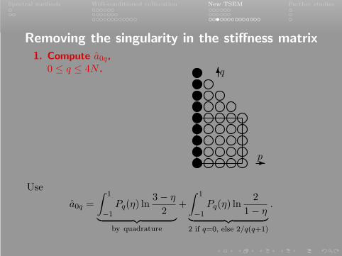
Removing the singularity in the stiffness matrix
1. Compute a0q,0 ≤ q ≤ 4N . q
p
Use
a0q =
∫ 1
−1Pq(η) ln
3− η
2︸ ︷︷ ︸by quadrature
+
∫ 1
−1Pq(η) ln
2
1− η︸ ︷︷ ︸2 if q=0, else 2/q(q+1)
.
Spectral methods Well-conditioned collocation New TSEM Further studies
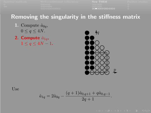
Removing the singularity in the stiffness matrix
1. Compute a0q,0 ≤ q ≤ 4N .
2. Compute a1q,1 ≤ q ≤ 4N − 1.
q
p
Use
a1q = 2a0q −(q + 1)a0,q+1 + qa0,q−1
2q + 1.
Spectral methods Well-conditioned collocation New TSEM Further studies
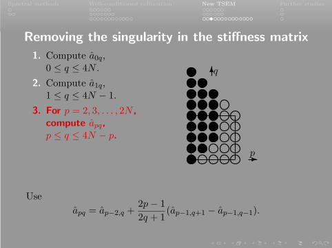
Removing the singularity in the stiffness matrix
1. Compute a0q,0 ≤ q ≤ 4N .
2. Compute a1q,1 ≤ q ≤ 4N − 1.
3. For p = 2, 3, . . . , 2N ,
compute apq,p ≤ q ≤ 4N − p.
q
p
Use
apq = ap−2,q +2p− 1
2q + 1(ap−1,q+1 − ap−1,q−1).
Spectral methods Well-conditioned collocation New TSEM Further studies
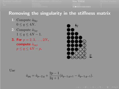
Removing the singularity in the stiffness matrix
1. Compute a0q,0 ≤ q ≤ 4N .
2. Compute a1q,1 ≤ q ≤ 4N − 1.
3. For p = 2, 3, . . . , 2N ,
compute apq,p ≤ q ≤ 4N − p.
q
p
Use
apq = ap−2,q +2p− 1
2q + 1(ap−1,q+1 − ap−1,q−1).
Spectral methods Well-conditioned collocation New TSEM Further studies
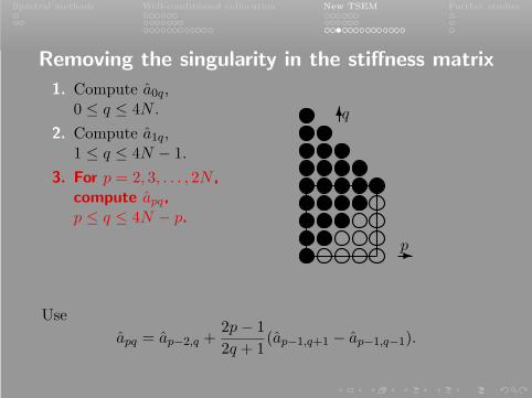
Removing the singularity in the stiffness matrix
1. Compute a0q,0 ≤ q ≤ 4N .
2. Compute a1q,1 ≤ q ≤ 4N − 1.
3. For p = 2, 3, . . . , 2N ,
compute apq,p ≤ q ≤ 4N − p.
q
p
Use
apq = ap−2,q +2p− 1
2q + 1(ap−1,q+1 − ap−1,q−1).
Spectral methods Well-conditioned collocation New TSEM Further studies
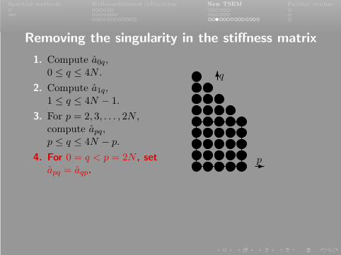
Removing the singularity in the stiffness matrix
1. Compute a0q,0 ≤ q ≤ 4N .
2. Compute a1q,1 ≤ q ≤ 4N − 1.
3. For p = 2, 3, . . . , 2N ,compute apq,p ≤ q ≤ 4N − p.
4. For 0 = q < p = 2N , set
apq = aqp.
q
p
Spectral methods Well-conditioned collocation New TSEM Further studies
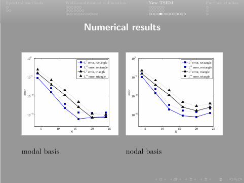
Numerical resultsConsider the elliptic equation:
−∆u+u = f in ; u|Γ1= 0;
∂u
∂~n
∣∣∣Γ2
= g,
where Γ1 is the edges x = 0 and y = 0, Γ2 is the hypotenuse of, and with the exact solution:
u(x, y) = ex+y−1 sin(3xy
(y −
√32 x+
√34
)).
For comparison, consider
−∆u+u = f in S = (0, 1/√2)2; u|Γ′
1= 0;
∂u
∂~n
∣∣∣Γ′
2
= g,
where Γ′1 is the edges x = 0 and y = 0 and Γ′
2 is the edgesx = 1/
√2 and y = 1/
√2, with exact solution
u(x, y) = exp(−(
1√2− x)(
1√2− y))
sin(3xy
(y −
√32 x+
√34
)).
Spectral methods Well-conditioned collocation New TSEM Further studies
Numerical results
5 10 15 20 25
10−15
10−10
10−5
100
N
erro
r
L2 error, rectangle
L∞ error, rectangle
L2 error, triangle
L∞ error, triangle
modal basis
5 10 15 20 25
10−15
10−10
10−5
100
Ner
ror
L2 error, rectangle
L∞ error, rectangle
L2 error, triangle
L∞ error, triangle
nodal basis
Spectral methods Well-conditioned collocation New TSEM Further studies
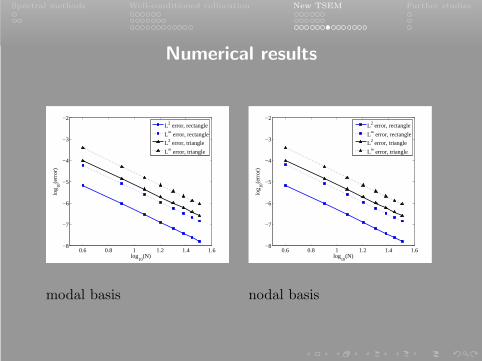
Numerical results
Consider the elliptic equation:
−∆u+u = f in ; u|Γ1= 0;
∂u
∂~n
∣∣∣Γ2
= g,
where Γ1 is the edges x = 0 and y = 0, Γ2 is the hypotenuse of, with the finite regularity exact solution:
u(x, y) = (1− x− y)52 (exy − 1) ∈ H3−ǫ()
The counterpart on the square S takes the form:
u(x, y) =
(1√2− x
) 52(
1√2− y
) 52
(exy − 1), ∀ (x, y) ∈ S.
Spectral methods Well-conditioned collocation New TSEM Further studies
Numerical results
0.6 0.8 1 1.2 1.4 1.6−8
−7
−6
−5
−4
−3
−2
log10
(N)
log 10
(err
or)
L2 error, rectangle
L∞ error, rectangle
L2 error, triangle
L∞ error, triangle
modal basis
0.6 0.8 1 1.2 1.4 1.6−8
−7
−6
−5
−4
−3
−2
log10
(N)lo
g 10(e
rror
)
L2 error, rectangle
L∞ error, rectangle
L2 error, triangle
L∞ error, triangle
nodal basis
Spectral methods Well-conditioned collocation New TSEM Further studies
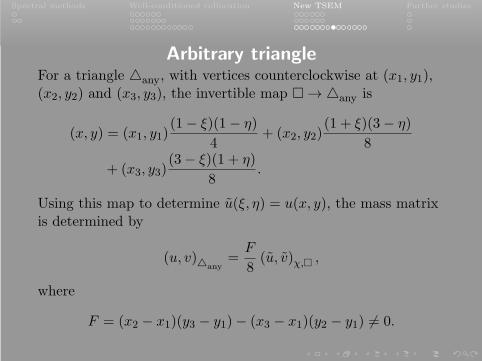
Arbitrary triangleFor a triangle any, with vertices counterclockwise at (x1, y1),(x2, y2) and (x3, y3), the invertible map → any is
(x, y) = (x1, y1)(1− ξ)(1− η)
4+ (x2, y2)
(1 + ξ)(3− η)
8
+ (x3, y3)(3− ξ)(1 + η)
8.
Using this map to determine u(ξ, η) = u(x, y), the mass matrixis determined by
(u, v)any=F
8(u, v)χ, ,
where
F = (x2 − x1)(y3 − y1)− (x3 − x1)(y2 − y1) 6= 0.
Spectral methods Well-conditioned collocation New TSEM Further studies
Arbitrary triangle
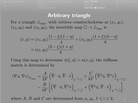
For a triangle any, with vertices counterclockwise at (x1, y1),(x2, y2) and (x3, y3), the invertible map → any is
(x, y) = (x1, y1)(1− ξ)(1− η)
4+ (x2, y2)
(1 + ξ)(3− η)
8
+ (x3, y3)(3− ξ)(1 + η)
8.
Using this map to determine u(ξ, η) = u(x, y), the stiffnessmatrix is determined by
(∇u,∇v)any=
A
2F
(∇ · u, ∇ · v
)χ−1,
+C
8F
(∇⊺u, ∇⊺v
)χ−1,
− B
4F
[(∇ · u, ∇⊺v
)χ−1,
+(∇⊺u, ∇ · v
)χ−1,
].
where A, B and C are determined from xi, yi, 1 ≤ i ≤ 3.
Spectral methods Well-conditioned collocation New TSEM Further studies
Unstructured TSEM with LDG-H
To use this TSEM on an unstructured mesh, the hybridized
local discontinuous Galerkin method is used.
• DG methods enjoy a large degree of flexibility,non-conformity and locality. In particular, DG methods
can handle hanging nodes in meshes, while providing ascheme to handle the coupling on the mesh. Having thehanging node in a predictable position allows for efficientcomputation.
• LDG-H makes use of auxillary functions, which renders theelliptic problem into a system of first-order differentialequations. For those inner products, the rectangle-triangle
map does not induce a singularity.
• LDG-H generates a global system whose degrees of
freedom are only those on the interior edges.
Spectral methods Well-conditioned collocation New TSEM Further studies
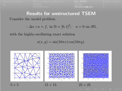
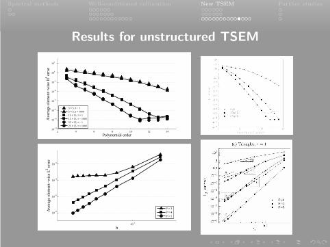
Results for unstructured TSEMConsider the model problem
−∆u+u = f, in Ω = [0, 1]2; u = 0 on ∂Ω,
with the highly-oscillating exact solution
u(x, y) = sin(10πx) cos(10πy).
0 0.2 0.4 0.6 0.8 10
0.2
0.4
0.6
0.8
1
x
y
5× 5
0 0.2 0.4 0.6 0.8 10
0.2
0.4
0.6
0.8
1
x
y
15× 15
0 0.2 0.4 0.6 0.8 10
0.2
0.4
0.6
0.8
1
xy
25× 25
Spectral methods Well-conditioned collocation New TSEM Further studies
Spectral methods Well-conditioned collocation New TSEM Further studies
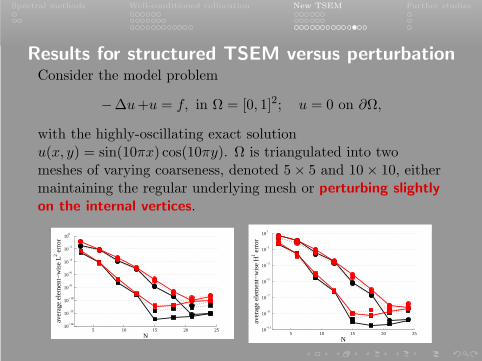
Results for structured TSEM versus perturbationConsider the model problem
−∆u+u = f, in Ω = [0, 1]2; u = 0 on ∂Ω,
with the highly-oscillating exact solutionu(x, y) = sin(10πx) cos(10πy). Ω is triangulated into twomeshes of varying coarseness, denoted 5× 5 and 10× 10, eithermaintaining the regular underlying mesh or perturbing slightly
on the internal vertices.
5 10 15 20 25
10−12
10−14
10−10
10−8
10−6
10−4
10−2
100
N
aver
age
elem
ent−
wis
e L
2 err
or
5 10 15 20 25
10−9
10−11
10−7
10−5
10−3
10−1
101
N
aver
age
elem
ent−
wis
e H
1 err
or
Spectral methods Well-conditioned collocation New TSEM Further studies
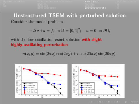
Unstructured TSEM with perturbed solutionConsider the model problem
−∆u+u = f, in Ω = [0, 1]2; u = 0 on ∂Ω,
with the low-oscillation exact solution with slight
Spectral methods Well-conditioned collocation New TSEM Further studies
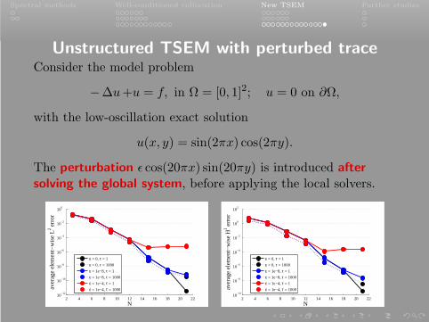
Unstructured TSEM with perturbed traceConsider the model problem
−∆u+u = f, in Ω = [0, 1]2; u = 0 on ∂Ω,
with the low-oscillation exact solution
u(x, y) = sin(2πx) cos(2πy).
The perturbation ǫ cos(20πx) sin(20πy) is introduced after
solving the global system, before applying the local solvers.
2 4 6 8 10 12 14 16 18 20 2210
−12
10−10
10−8
10−6
10−4
10−2
100
N
aver
age
elem
ent−
wis
e L
2 err
or
ε = 0, τ = 1
ε = 0, τ = 1000
ε = 1e−8, τ = 1
ε = 1e−8, τ = 1000
ε = 1e−4, τ = 1
ε = 1e−4, τ = 1000
2 4 6 8 10 12 14 16 18 20 2210
−10
10−8
10−6
10−4
10−2
100
102
N
aver
age
elem
ent−
wis
e H
1 err
or
ε = 0, τ = 1
ε = 0, τ = 1000
ε = 1e−8, τ = 1
ε = 1e−8, τ = 1000
ε = 1e−4, τ = 1
ε = 1e−4, τ = 1000
Spectral methods Well-conditioned collocation New TSEM Further studies
Well-conditioned collocation
Research for the method in the first part, which produceswell-conditioned collocation schemes, three directions areworthy of further investigation.
• Investigate the notion for well-conditionedpolynomial-based collocation methods for other situations,e.g., the spline collocation, radial basis functions and somenon-polynomial bases.
• Extension of the well-conditioned collocation approach tomultiple dimensions.
• Obtain the optimal error estimates for the Birkhoffinterpolations.
Spectral methods Well-conditioned collocation New TSEM Further studies
Tetrahedral spectral elements
The new TSEM on unstructured meshes based on the DGformulation is worthy of deep investigation. Furtherdevelopment can be taken in the following directions:
• Apply the TSEM to more challenging problems such as theStokes equations and the Navier-Stokes equations.
• Develop a three-dimensional unstructured tetrahedralTSEM.
• Prove global convergence of the unstructured TSEM.
Spectral methods Well-conditioned collocation New TSEM Further studies
Further reading
Robert Kirby, Spencer Sherwin and Bernardo Cockburn. ToCG or to HDG: a comparative study. Journal of ScientificComputing, vol. 51 (1), 183–212, 2012
Michael Daniel Samson, Li-Lian Wang and Huiyuan Li. Anew triangular spectral element method I:
implementation and analysis on a triangle. NumericalAlgorithms, vol. 64 (3), 519–547, 2013
Li-Lian Wang, Michael Daniel Samson and Xiaodan Zhao.A well-conditioned collocation method using a
pseudospectral integration matrix. Accepted to SIAMJournal on Scientific Computing, 2014