1 Tishk International University Engineering Faculty Petroleum and Mining Department Well Testing 4-Grade- Spring Semester 2020-2021 Lecture 6: Fluid Flow in Porous Media Instructor: Frzan Ali Frzan Ali / 2020 - 2021
Transcript
1
Tishk International UniversityEngineering FacultyPetroleum and Mining Department
Well Testing
4-Grade- Spring Semester 2020-2021
Lecture 6: Fluid Flow in Porous Media
Instructor: Frzan AliFrzan Ali / 2020 - 2021
Content
Frzan Ali
Well Testing2
• Flow Regimes
• Unsteady (Transient) -State Flow
• Development of Radial Differential Equation
• Solution to Diffusivity Equation
• Solution to Diffusivity Equation-Transient Flow
Flow Regimes
• Under the steady-state flowing condition, the same quantity of fluid enters the flow system as leaves it.
• In the unsteady-state flow condition, the flow rate into an element of volume of a porous media may not be the same as the flow rate out of that element.
• Accordingly, the fluid content of the porous medium changes with time.
• The variables in unsteady-state flow additional to those already used for steady-state flow, therefore, become:
• Time
• Porosity
• Fluid viscosity
• Total compressibility (Rock and fluid)
Frzan Ali
Well Testing3
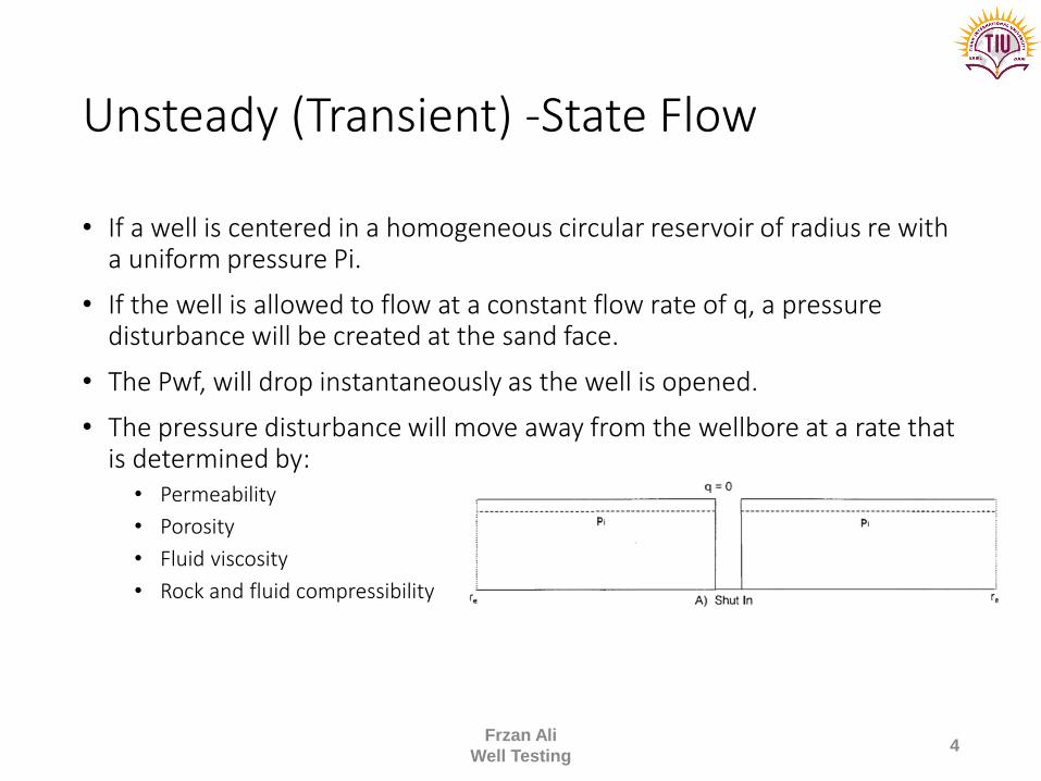
Unsteady (Transient) -State Flow
• If a well is centered in a homogeneous circular reservoir of radius re with a uniform pressure Pi.
• If the well is allowed to flow at a constant flow rate of q, a pressure disturbance will be created at the sand face.
• The Pwf, will drop instantaneously as the well is opened.
• The pressure disturbance will move away from the wellbore at a rate that is determined by:
• Permeability
• Porosity
• Fluid viscosity
• Rock and fluid compressibility
Frzan Ali
Well Testing4
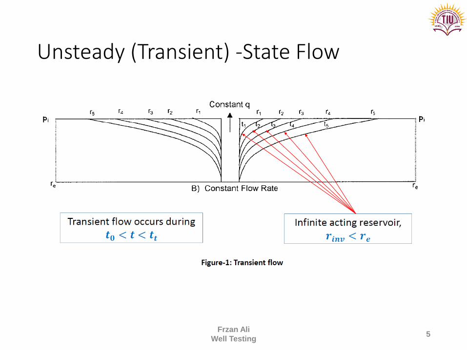
Unsteady (Transient) -State Flow
Frzan Ali
Well Testing5
Unsteady (Transient) -State Flow
Frzan Ali
Well Testing6
Transient (unsteady-state) flow is defined asThat time period during which the boundary has no effect on the pressure behavior in the reservoir and the reservoir will behave as its infinite in size
Development of Radial Differential Equation
Frzan Ali
Well Testing7
Development of Radial Differential Equation
Ideal Reservoir Model
• Developing analysis techniques for well testing requires assumptions.
• The assumptions are introduced to combine the followings:• Law of mass conservation (continuity equation).
• Darcy law.
• Compressibility equation.
• Initial and boundary conditions.
Frzan Ali
Well Testing8
Development of Radial Differential Equation
Continuity Equation• The continuity equation is essentially a material balance equation that accounts for
every pound mass of fluid produced, injected, or remaining in the reservoir.
Transport Equation• The continuity equation is combined with the equation for fluid motion (transport
equation) to describe the fluid flow rate “in” and “out” of the reservoir. Basically, the transport equation is Darcy’s equation in its generalized differential form.
Compressibility Equation• The fluid compressibility equation (expressed in terms of density or volume) is used in
formulating the unsteady-state equation with the objective of describing the changes in the fluid volume as a function of pressure.
Initial and Boundary Conditions• There are two boundary conditions and one initial condition required to complete the
formulation and the solution of the transient flow equation. The two boundary
Frzan Ali
Well Testing9
Development of Radial Differential Equation
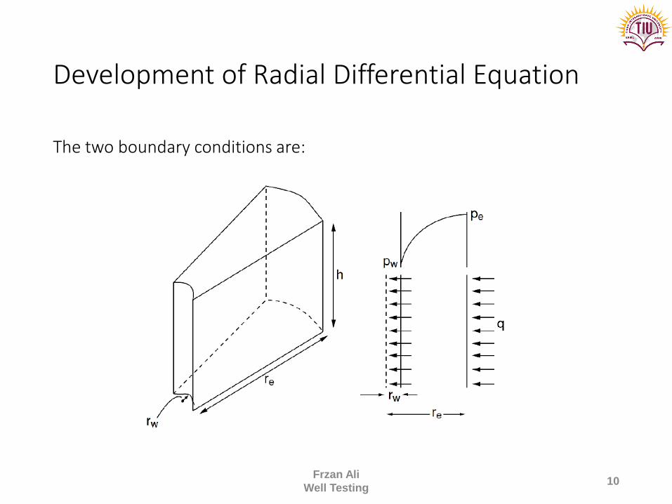
The two boundary conditions are:
Frzan Ali
Well Testing10
Development of Radial Differential Equation
• According to the concept of the material-balance equation
• The rate of mass flow into and out of the element during a differential time Δt must be equal to the mass rate of accumulation during that time interval
Frzan Ali
Well Testing11
Development of Radial Differential Equation
Frzan Ali
Well Testing12
Development of Radial Differential Equation
Frzan Ali
Well Testing13
Development of Radial Differential Equation
Frzan Ali
Well Testing14
Development of Radial Differential Equation
Frzan Ali
Well Testing15
Development of Radial Differential Equation
Frzan Ali
Well Testing16
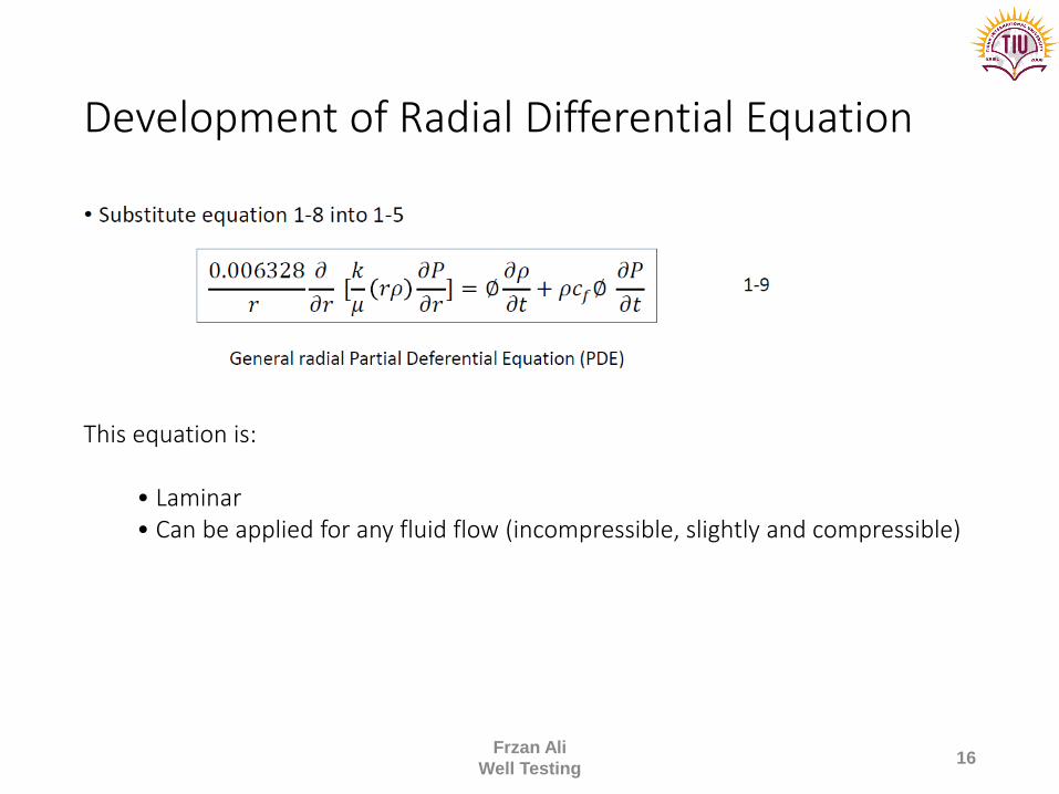
This equation is:
• Laminar• Can be applied for any fluid flow (incompressible, slightly and compressible)
Development of Radial Differential Equation
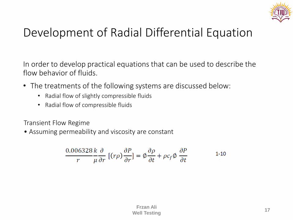
In order to develop practical equations that can be used to describe the flow behavior of fluids.
• The treatments of the following systems are discussed below:• Radial flow of slightly compressible fluids
• Radial flow of compressible fluids
Frzan Ali
Well Testing17
Transient Flow Regime• Assuming permeability and viscosity are constant
Development of Radial Differential Equation
Frzan Ali
Well Testing18
Development of Radial Differential Equation
Frzan Ali
Well Testing19
Development of Radial Differential Equation
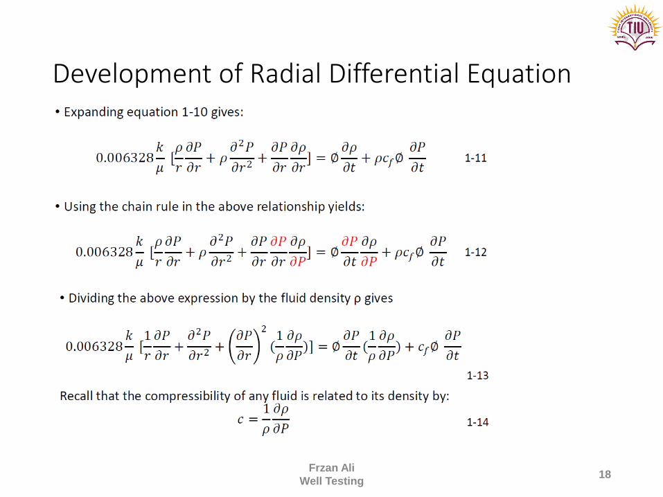
Equation 1-18 is called the Diffusivity Equation
The equation is particularly used in analysis well testing data where the time t is commonly recorded in hours.
Frzan Ali
Well Testing20
Development of Radial Differential Equation
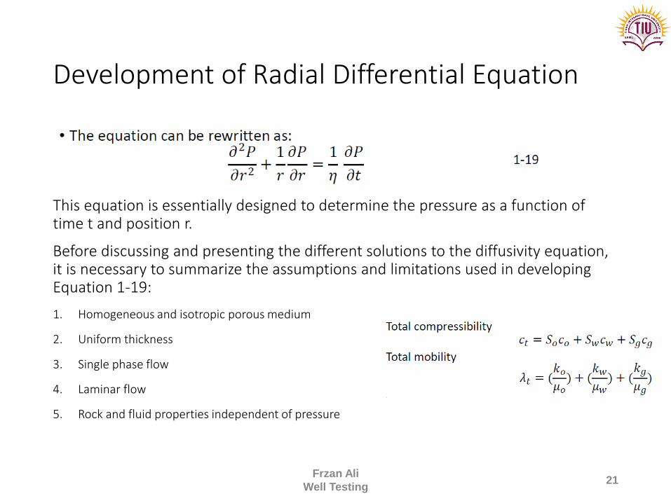
This equation is essentially designed to determine the pressure as a function of time t and position r.
Before discussing and presenting the different solutions to the diffusivity equation, it is necessary to summarize the assumptions and limitations used in developing Equation 1-19:
1. Homogeneous and isotropic porous medium
2. Uniform thickness
3. Single phase flow
4. Laminar flow
5. Rock and fluid properties independent of pressure
Frzan Ali
Well Testing21
Solution to Diffusivity Equation
• For a steady-state flow condition, the pressure at any point in the reservoir is constant and does not change with time, i.e., ∂p/∂t = 0, and therefore Equation 1-19 reduces to:
Frzan Ali
Well Testing22
Solution to Diffusivity Equation
• Solution for the following flow regimes:• Steady-state
• Pseudo-steady-state
• Unsteady-state
• To obtain a solution to the diffusivity equation (Equation 1-19), it is necessary to specify:
• Initial condition: states that the reservoir is at a uniform pressure pi when production begins.
• The two boundary conditions: require that the well is producing at a constant production rate and that the reservoir behaves as if it were infinite in size
Frzan Ali
Well Testing23
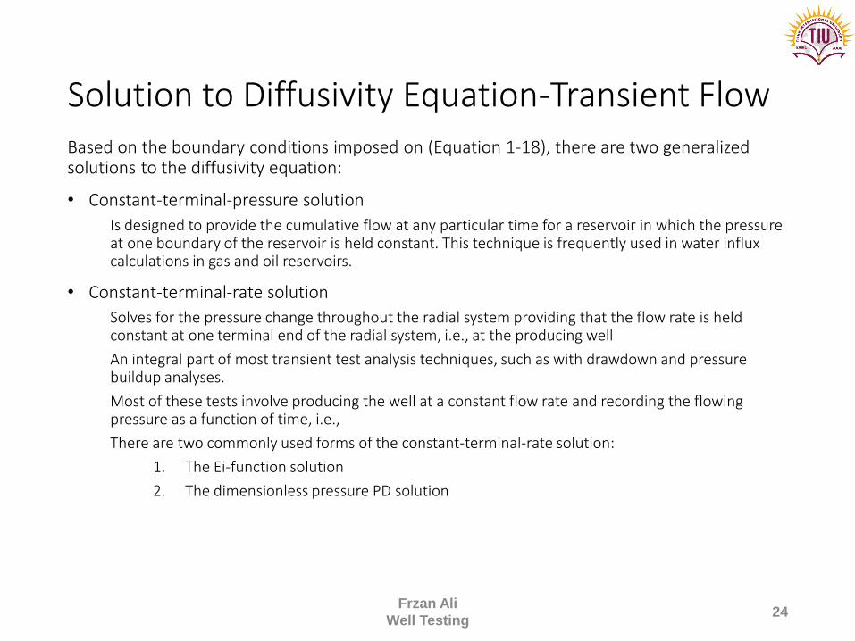
Solution to Diffusivity Equation-Transient FlowBased on the boundary conditions imposed on (Equation 1-18), there are two generalized solutions to the diffusivity equation:
• Constant-terminal-pressure solution
Is designed to provide the cumulative flow at any particular time for a reservoir in which the pressure at one boundary of the reservoir is held constant. This technique is frequently used in water influx calculations in gas and oil reservoirs.
• Constant-terminal-rate solution
Solves for the pressure change throughout the radial system providing that the flow rate is held constant at one terminal end of the radial system, i.e., at the producing well
An integral part of most transient test analysis techniques, such as with drawdown and pressure buildup analyses.
Most of these tests involve producing the well at a constant flow rate and recording the flowing pressure as a function of time, i.e.,
There are two commonly used forms of the constant-terminal-rate solution:
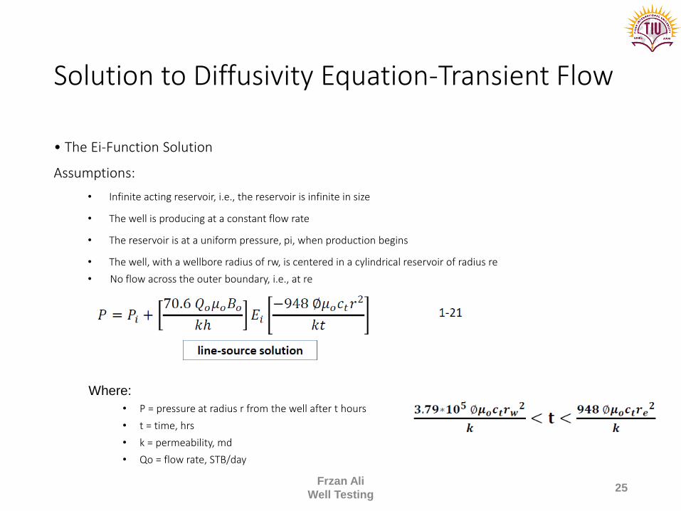
1. The Ei-function solution
2. The dimensionless pressure PD solution
Frzan Ali
Well Testing24
Solution to Diffusivity Equation-Transient Flow
• The Ei-Function Solution
Assumptions:
• Infinite acting reservoir, i.e., the reservoir is infinite in size
• The well is producing at a constant flow rate
• The reservoir is at a uniform pressure, pi, when production begins
• The well, with a wellbore radius of rw, is centered in a cylindrical reservoir of radius re
• No flow across the outer boundary, i.e., at re
Frzan Ali
Well Testing25
Where:
• P = pressure at radius r from the well after t hours
• t = time, hrs
• k = permeability, md
• Qo = flow rate, STB/day
Solution to Diffusivity Equation-Transient Flow
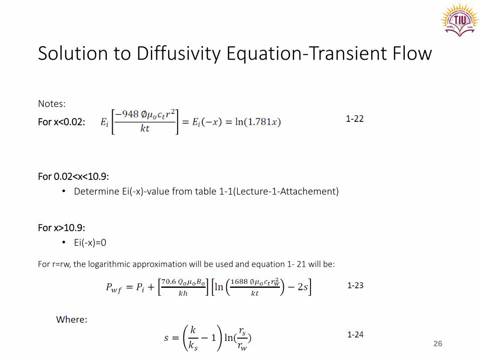
Notes:
For x<0.02:
For 0.02<x<10.9:
• Determine Ei(-x)-value from table 1-1(Lecture-1-Attachement)
For x>10.9:
• Ei(-x)=0
Frzan Ali
Well Testing26
For r=rw, the logarithmic approximation will be used and equation 1- 21 will be:
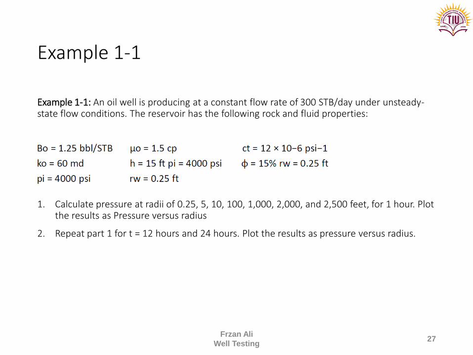
Example 1-1
Example 1-1: An oil well is producing at a constant flow rate of 300 STB/day under unsteady-state flow conditions. The reservoir has the following rock and fluid properties:
Frzan Ali
Well Testing27
1. Calculate pressure at radii of 0.25, 5, 10, 100, 1,000, 2,000, and 2,500 feet, for 1 hour. Plot the results as Pressure versus radius
2. Repeat part 1 for t = 12 hours and 24 hours. Plot the results as pressure versus radius.
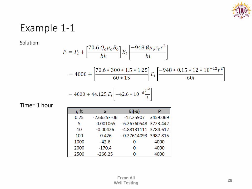
Example 1-1Solution:
Frzan Ali
Well Testing28
Time= 1 hour
Example 1-1
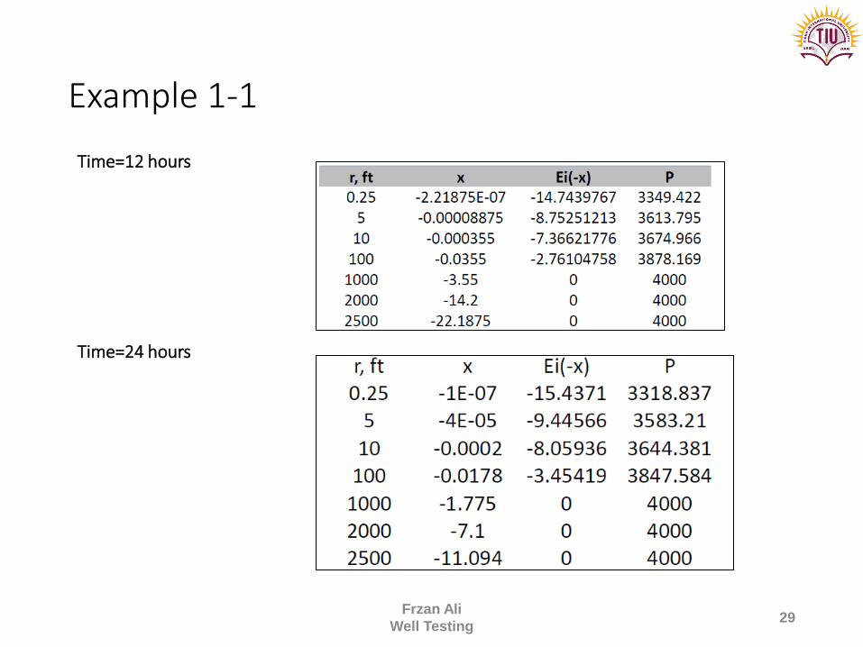
Time=12 hours
Frzan Ali
Well Testing29
Time=24 hours
Example 1-1
Frzan Ali
Well Testing30
Example 1-2
Example 1-2: for an oil well producing at constant rate of 10 SRB/day. Blow are the description data for the well and the reservoir.
Frzan Ali
Well Testing31
Calculate the reservoir pressure at radius of 1, 10 and 100 ft after 3 hours of production.
Example 1-2Solution:
Frzan Ali
Well Testing32
The end time for the reservoir to act as infinite reservoir is given by:
The reservoir will act as infinite reservoir till the time of 𝟐𝟏𝟏, 𝟗𝟎𝟎𝟎 ℎ𝑟𝑠