Electronic copy available at: http://ssrn.com/abstract=1455161

Were Mankiw, Romer, and Weil Right? A Reconcilation of the Micro and Macro Effects

of Schooling on Income

Theodore R. Breton*

October 3, 2011

Abstract

The marginal product of human capital in Mankiw, Romer, and Weil’s [1992] augmented Solow

model measures the direct and two external effects of human capital created from schooling on

national income. If this model is valid, its estimates of the share of this marginal product

accruing to workers should be consistent with estimates of the marginal return on investment in

schooling in workers’ earnings’ studies. This paper uses a new set of data for the net human

capital stock to show that in 1990 the micro and macro rates are consistent across 36 countries.

JEL Codes: E13, I21, O11, O15, O41

Key Words: Human Capital, Education, Schooling, Neoclassical Model, Economic Growth

*Thanks to George Psacharopoulos and Asa Janney for assistance and to Steven Davis, Andrew

Breton, Charles Mann, and numerous anonymous referees for comments on earlier versions of

this paper.

Electronic copy available at: http://ssrn.com/abstract=1455161

2

When Mankiw Romer, and Weil [1992] added human capital from schooling to the

Solow model, it solved several empirical problems. This addition enabled the model to explain

the differences in income across countries, to provide an accurate estimate of the share of

national income accruing to physical capital, and to provide a more accurate representation of the

rate of income convergence in response to changes in rates of capital investment. But it also

revealed a statistical relationship that many found problematic – a very large effect of human

capital on national income.

In Mankiw, Romer, and Weil’s version of the Solow model (hereafter denoted the MRW

model), productivity (A) varies over time, but country-specific differences affecting productivity

not related to physical or human capital levels are assumed to be random:1

(1) (Y/L)it = (K/L)it α (

H/L)it β (At

)

1-α-β

MRW’s empirical results, since replicated by other researchers2, indicate that differences in

physical capital (K) and human capital (H) can explain almost all of the variation in national

income (Y) across countries, leaving little or no variation to be explained directly by other

factors. In this model the levels of physical capital and human capital are the proximate

determinants of national income. Other national characteristics, including institutions, policies,

and culture, affect income through their effect on these capital factors.3

Critics have argued that the MRW model is mis-specified because it does not include any

of these national characteristics, but the evidence supporting the inclusion of other variables is

weak. Levine and Renelt [1992] examined the relationship between over 50 variables and

1 For example, hours worked per year vary across countries but are not included as a control variable.

2Cohen and Soto [2007] obtain similar estimates of the model within countries between 1960 and 1990. Breton

[2010] obtains similar estimates across countries for the period 1990-2000.

3 Mauro [1995] presented evidence that a measure of a country’s bureaucratic efficiency, which has since been

interpreted to measure either a country’s institutions or its policies, affects its level of physical capital.

Electronic copy available at: http://ssrn.com/abstract=1455161

3

growth and found that over the 1960-89 period only investment in physical capital is robustly

correlated with growth. Ciccone and Jarocinski [2010] have investigated whether 67 variables

are correlated with growth and found that over the 1960-96 period only education variables are

robustly linked with growth.

Klenow and Rodriguez-Clare [1997] and Hall and Jones [1999] have contributed to the

perception that variables are omitted from the model. They presented analyses that purportedly

show that the effect of schooling on workers’ earnings in micro studies is much smaller than the

effect in MRW’s empirical results. They estimated the average effect of schooling on earnings

in micro studies and then subtracted these earnings and their estimate of the effect of physical

capital from national income in each country to estimate country-specific productivity residuals

(Ai). Klenow and Rodriguez-Clare used the MRW model to estimate this residual, while Hall

and Jones used a slightly different model, but both analyses show that national differences in

productivity (Ai) have a larger effect on national income than differences in workers’ earnings

related to schooling.

Both sets of authors demonstrate that their productivity residuals are highly correlated

with human capital. Klenow and Rodriguez-Clare acknowledge that these residuals could be an

external effect of human capital related to the speed of technology diffusion, but they show that

for the MRW empirical results to be valid, this effect would have to be much larger than the

direct effect on workers’ earnings. Hall and Jones argue that the productivity residuals are

caused by differences in institutions and government policies, and they present statistical

evidence to support this view. These papers’ influence in undermining support for MRW’s

model is unfortunate because the methodology the authors used to calculate their productivity

residuals is flawed.

4

The MRW model presumes that physical capital and skill are complementary. An

increase in the level of one capital factor increases the marginal product of the other capital

factor. In any model with a multiplicative relationship between the two forms of capital, the

external effects of human capital (and physical capital) are an integral part of the model, and any

comparison of the effect of schooling in micro studies with the empirical results in these models

must account for these external effects. Due to the complementary effect of skill on (physical)

capital, only part of the marginal product of human capital accrues to workers. Since they did

not take this into account, Klenow and Rodriguez-Clare and Hall and Jones substantially

overestimated the productivity residuals (Ai) remaining after subtracting the independent

estimates of schooling and physical capital from national income.

As shown later in this paper, in MRW’s model the aggregate external effect of human

capital is (1-β)/β times the direct effect. Given the independent estimate that α is approximately

0.35, the Cobb-Douglas structure with constant returns ensures that β ≤ 0.65. As a result, the

aggregate external effect of human capital in the model is at least 0.54 times the direct effect

(.35/.65) and possibly much higher. With MRW’s estimate of β = 0.3, the external effect of

human capital in the MRW model is 2.3 times the direct effect.

The large external effect of human capital inherent in the MRW model (and in Hall and

Jones’ model) is either a great strength or a great weakness. But it is not an optional effect, and

it cannot be ignored when examining whether MRW’s empirical results are consistent with

micro estimates of the effect of schooling on workers’ earnings.

In the MRW model human capital (H) has two external effects, one on physical capital

(K) and one on labor (L), both of which are mathematically specified. This defined relationship

suggests a test of the model’s validity. Since workers receive income from human capital

5

through the direct effect (β) and the external effect (1-α-β) on labor, their total income must be

bounded by the direct effect on the low side and by the sum of these two effects on the high side.

If the MRW model is valid, the independent estimates of workers’ incomes must fall within these

bounds.

This paper presents the results of such a test. It compares the estimates of the upper and

lower bounds of the share of the marginal product of human capital accruing to workers in the

MRW model with estimates of the marginal product of schooling in existing micro studies in 36

countries. Conceptually, Klenow and Rodriguez-Clare [1997] and Hall and Jones [1999]

performed a similar test, but their implementation of this test was flawed.

If the marginal product of human capital in the macro model is consistent with the

marginal product of schooling in the micro studies, then MRW’s model, including its large

external effects of human capital, is not rejected. If MRW’s model is valid, then institutions and

policies affect national income indirectly through their effect on the levels of capital, and they

are not omitted variables in their model.

This test of the MRW model is a stringent one. The Cobb-Douglas structure with two

capital variables is quite constraining. Conceptually the exponents on the two capital stocks are

both 1) the marginal effect on national income of an increase in the stock of each type of capital

and 2) the share of any increase in national income that accrues either directly or indirectly to

that type of capital as a result of an increase in any factor. If the MRW model can explain the

distribution of national income across countries and the share of this income that has accrued to

each factor of production in these countries, this is a significant achievement.

In order to perform this test, I develop new cross-country estimates of the marginal

product of human capital in the MRW model in 1990. I estimate the model with a new set of

6

human capital data that is based on each country’s cumulative investment in schooling, adjusted

for purchasing power parity. My financial measure of human capital is conceptually identical to

standard measures of the stock of physical capital. This measure eliminates many of the

estimation issues associated with proxies for human capital, such as years of schooling, which

may not be a consistent measure across countries. I include foregone student earnings in both

the human capital and the national income data. Subsequently, I estimate the marginal product

of schooling in micro studies of workers’ earnings in 36 countries from the 1986-94 period and

compare these estimates to the relevant shares of the marginal product of human capital in the

MRW model in the same 36 countries.

In contrast to Klenow and Rodriguez-Clare [1997] and Hall and Jones [1999], I find that

the estimates of the effect of schooling in MRW’s model are consistent with the estimates of the

effect of schooling in micro studies. In the lowest-income countries, the marginal product in

micro studies is equal to the direct share of the marginal product of human capital (i.e., the share

β that accrues to the human capital factor). In the highest-income countries, the marginal

product in micro studies is equal to this direct share plus most of the external share that accrues

to labor (i.e., the 1-α share). These empirical results indicate that as a country’s level of human

capital rises, a growing share of the external effect of schooling accrues to the educated portion

of the work force.

This paper makes several contributions to the literature. First, it provides a conceptual

framework for comparing the macro and the micro effects of schooling on income, two strands

of the economics literature that previously have not been reconciled. Second, it provides

estimates of the net stock of human capital from schooling and the marginal product of human

capital from schooling for 61 countries in 1990. Third, it shows that the marginal product of

7

human capital in the augmented Solow growth model is consistent with the marginal product of

schooling in workers’ earnings’ studies.

The paper is organized as follows: Section I describes the methodology used to create

the two sets of rates. Section II develops estimates of the net stock of human capital from

schooling. Section III develops new estimates of α and β. Section IV develops national average

marginal products of schooling from rates of return on investment in schooling in workers’

earnings studies. Section V compares the micro and macro marginal products of schooling for

these countries. Section VI concludes.

I. Methodological Considerations

The rates of return in workers’ earnings studies and the marginal product in the Cobb-

Douglas national income model are similar in that they both are marginal rates. Both of them

estimate the effect of an increase in schooling on income in one year and convert this effect into

a marginal product. Despite these similarities, there are differences between these rates that must

be addressed to make them comparable:

1) The macro rates include the national income that accrues to workers and to

physical capital, while the micro rates include only the part that accrues to workers.

2) The average experience of the workers is not the same in the two analyses. The

micro rates assume a level of experience that is the average over a worker’s life.

The macro rates implicitly are based on a lower average level of experience due to

the historic growth of the population across countries.

3) The micro rates implicitly or explicitly account for students’ foregone earnings,

while data on national income exclude these earnings.

8

4) The micro financial rates of return are estimated for schooling at the primary, the

secondary, and the university levels, while the macro rates estimate the marginal

product on aggregate investment in schooling at all levels.

5) Some of the micro rates are estimated using the Mincerian methodology, which

estimates wage effects from increases in years of schooling rather than financial

rates of return [Psacharopoulos and Patrinos, 2004].

In this paper I adjust the input data or the macro and micro estimates of the marginal

product of schooling to account for these differences, so that the final estimates are comparable

from a conceptual standpoint. To further ensure comparability I develop the macro and micro

estimates for the same period of time. The marginal product of schooling in the workers’ studies

is estimated for 36 countries for which data were available for the 1986-94 period. The relevant

shares of the marginal product of human capital in the macro model are estimated for the same

countries using data for 1990, the mid-point in the period used for the micro rates. The use of a

financial measure for human capital in the macro analysis facilitates the reconciliation of the

macro marginal product with the financial rates of return in the micro studies.

Macro Rates of Return

The principal conceptual issue in the analysis is the identification of the share of the

marginal product of schooling in the MRW model that is comparable to the rates of return on

investment in workers’ earnings studies. This share can be identified because the Cobb-Douglas

structure in equation (1) provides an explicit distribution of the national income from the

marginal product of human capital to the three factors of production.

The marginal product of human capital in the MRW model is:

(2) MPH = δYi /δHi = β Yi /Hi

9

As is shown below, in the Cobb-Douglas production function, the share of the marginal product

of schooling that accrues to each factor of production is equal to the exponent on that factor.

As the marginal product is a partial derivative, it holds the stocks of physical capital and

labor constant. As a result, the increase in national income that accrues to physical capital and

labor is provided through an increase in the return (Δrk) on physical capital4 and an increase in

the wage (Δw) paid to labor. The increase in income that accrues to human capital from

schooling is the net result of the increase in the stock of human capital and the decline in the

return (rh) paid to this stock of capital due to diminishing returns (Δ(rhH)).

From an economic standpoint an increase in human capital raises the return to physical

capital and the wage paid to labor by increasing the productivity of these two factors through an

external or spillover effect. In the Cobb-Douglas model the wage paid to labor in a market

economy is equal to the marginal product of labor:

(3) wi = δYi /δLi = (1-α-β) Yi /Li

Mathematically, this wage is the share of national income that is left over (1-α-β) after the two

forms of capital receive their marginal returns. The wage (w) increases when either stock of

capital increases because the marginal products of physical capital and human capital in the

Cobb-Douglas model are less than the average products.

The wage (w) in the model is the average payment to the labor force resulting from the

external effects of physical capital and human capital that does not accrue to those two factors.

This wage (w) is separate from the payment made to workers to compensate them for their

4 While an increase in human capital from schooling raises the return on physical capital, in a market economy this

increase is theoretical. As incremental schooling raises the marginal product of physical capital, investment in

physical capital increases, which causes the marginal product to remain at the market rate of return. The share of

national income accruing to physical capital continues to equal α, but the higher income is then due to the increase

in the stock of physical capital rather than to the increase in its marginal product.

10

higher productivity related to their own level of schooling (rh). In the model in equation (1),

schooled workers receive both a labor wage (w) and the direct return on the nation’s investment

in their schooling (rh).

The Cobb-Douglas structure does not specify how the payments to workers from the

external effects (w) are distributed to workers with different levels of schooling (including to

workers with no schooling), nor does it require that these payments be distributed in the same

way across countries or within countries over time. If the change in the wage (Δw) caused by the

external effect of schooling is provided to all workers (L), then the incremental earnings that

schooled workers receive from incremental schooling will include only the direct return on

investment in schooling (rh). In this case the rate of return on schooling in workers’ earning

studies will be limited to the share of the marginal product of schooling in the macro model that

accrues to the recipients of schooling. This rate can be calculated as the partial derivative of the

national income paid to the human capital factor of production:

(4) rh = δ(rhi Hit)/δHi = δ((βYi /Hi) Hi)/δHi = β MPH = β2 Yi /Hi

The share of the marginal product that accrues to labor as an external effect of schooling

can be calculated as the partial derivative of the national income paid to the labor factor of

production (wL):

(5) Ext MPH to L = δ(wiLi)/δHi = δ((1-α-β)Yi/Li) Li)/δHi = (1-α-β) MPH = (1-α-β)β Yi /Hi

If the change in the wage (Δw) caused by the external effect of schooling is provided entirely to

workers who are schooled, then schooled workers’ earnings from incremental schooling will

include both the direct return and the external effect on w from investment in schooling. In this

11

case the measured return on investment in schooling in workers’ earning studies will include the

direct and the external shares of income that accrue to workers:5

(6) Direct + Ext MPH to Labor = (β MPH) + (1-α-β) MPH = (1-α) MPH = (1-α)β Yi /Hi

So equations (4) and (6) bound the rates of return that should be expected in workers’ earnings

studies if the MRW model is a valid model and if α and β are correctly estimated.

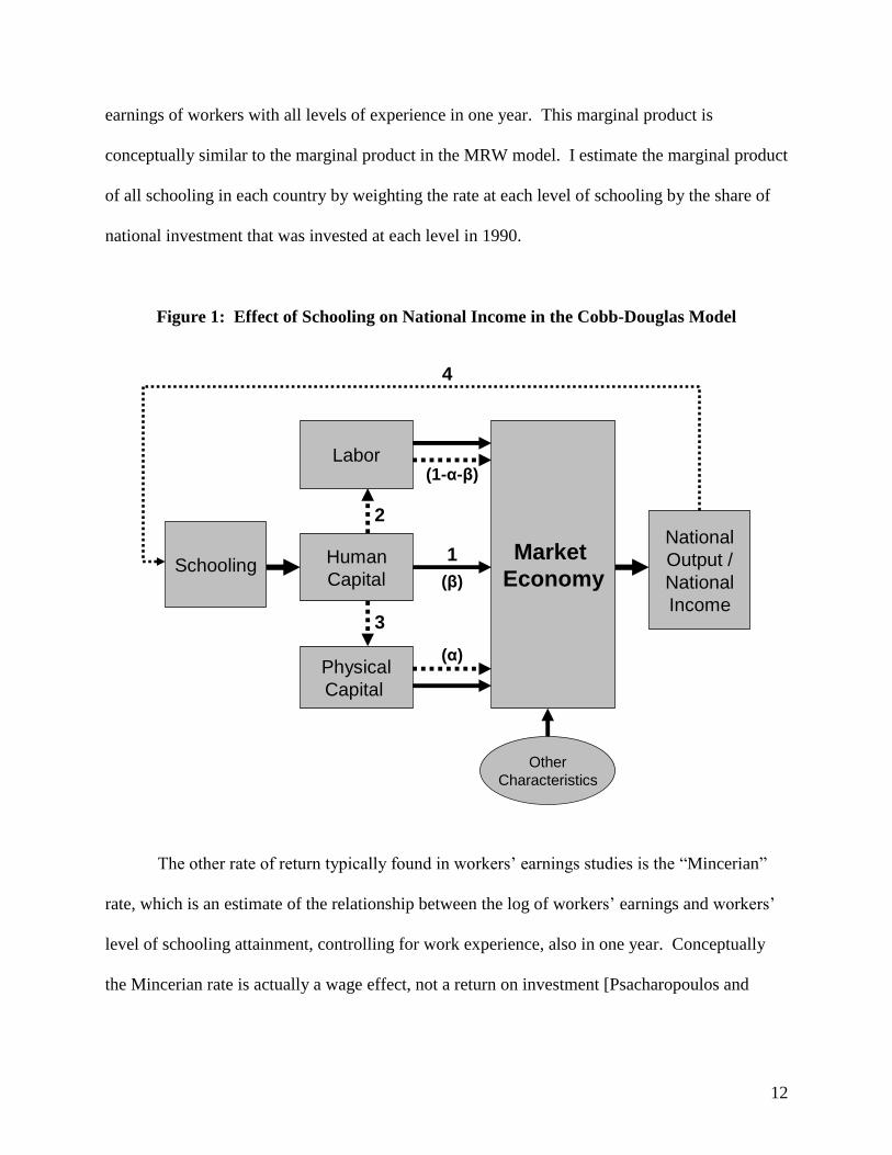
Figure 1 provides a schematic of how increased schooling affects national income in the

MRW model. The direct effect (1) is shown with a solid line, while the external or indirect

effects (2, 3, and 4) are shown with a dotted line. In this model the relative magnitudes of the

direct effect of schooling on national income and the two external effects (2 and 3) are

determined by the estimates of α and β. The external effects in the Cobb-Douglas model are (1-

β)/β times the direct effect, so unless β > 0.5, the external effects are larger than the direct effect.

Micro Rates of Return on Investment in Schooling

The rates of return on schooling estimated in workers’ earnings studies are typically of

two types. One type, which Psacharopoulos and Patrinos [2004] denote the “full return” rate, is

calculated using the standard internal rate of return methodology used in project analysis. This

rate is the discount rate that equalizes the present discounted value of the cost stream and the

income stream associated with incremental investment in schooling. The costs include the

expenditures on schooling and the students’ foregone earnings while they are in school. The

income is the incremental earnings associated with the incremental schooling over the life of the

worker.

But the full return rates estimated in the literature are not the actual return on investment

in schooling, which would be calculated over the life of the investment. These rates are actually

the marginal product of a certain level of schooling where income is defined as the average

5 The remaining share of the marginal product of human capital (α MPH = αβYi /Hi) accrues to physical capital.

12

earnings of workers with all levels of experience in one year. This marginal product is

conceptually similar to the marginal product in the MRW model. I estimate the marginal product

of all schooling in each country by weighting the rate at each level of schooling by the share of

national investment that was invested at each level in 1990.

Figure 1: Effect of Schooling on National Income in the Cobb-Douglas Model

Labor

Schooling

Physical

Capital

Market

Economy

National

Output /

National

Income

Other

Characteristics

1

3

(α)

4

(1-α-β)

Human

Capital

2

(β)

The other rate of return typically found in workers’ earnings studies is the “Mincerian”

rate, which is an estimate of the relationship between the log of workers’ earnings and workers’

level of schooling attainment, controlling for work experience, also in one year. Conceptually

the Mincerian rate is actually a wage effect, not a return on investment [Psacharopoulos and

13

Patrinos, 2004]. Calculation of the Mincerian rate requires less information than calculation of

the full return rate, so Mincerian rates are available for more countries than are full return rates.

The magnitude and the pattern of diminishing returns are very similar for the Mincerian

rates and for the marginal product of workers’ schooling calculated from the full return rates, so

workers’ marginal product of schooling can be estimated from the Mincerian rate. In this study

there are 16 countries for which there are both full return rates and Mincerian rates. I determine

the average ratio between the marginal products and the Mincerian rates and then use this ratio in

countries that had only a Mincerian rate to estimate their marginal product of schooling.6

II. Estimation of the Net Schooling Capital Stock

Calculation of the marginal product of human capital (MPH) in the MRW model requires

cross-country data on the stock of human capital. I estimate these stocks using the perpetual

inventory method specified in OECD [2001]. As far as I know, estimates of a nation’s stock of

human capital from its investment in schooling have not previously been developed.

The OECD argues that for financial valuation, the appropriate stock of capital is the net

capital stock, which includes all of the capital equipment in operation, with a value for this

capital that is either a market value, or is calculated using its initial cost (the gross capital stock)

and financial depreciation. I calculate each country’s gross human capital stock using its

aggregate investment in formal schooling, which includes all expenditures related to schooling,

financial carrying costs until the student enters the work force, and students’ foregone earnings.

I estimate these stocks in 1990 for 61 countries that had been market economies and for which

data on school expenditures are available for the 1950-85 period.

6 Critics have challenged the methodology used to estimate Mincerian rates because it incorrectly assumes that the

effects of schooling and experience on income are independent. Despite this conceptual deficiency, the method used

to estimate the full return rates from the Mincerian rates in this analysis is still valid.

14

In my estimates I assume that students complete their schooling and then work for 40

years. This working life is consistent with the life expectancy of children beginning school in all

countries, except in those sub-Saharan African countries that have a high incidence of AIDS or

other diseases.7

I assume that a country’s gross human capital stock from schooling in year t is equal to

its cumulative national investment in schooling over the years t-45 to t-5. The five-year lag is a

rough approximation of the delay from a present discounted value standpoint between the time

when a nation invests in schooling and the time that a student enters the work force. This lag is

less than half the average student’s period of schooling because higher levels of schooling have

much higher unit costs than lower levels of schooling [Breton, 2010]. I estimate the cumulative

investment using data at five-year intervals on public expenditures as a share of national income,

a national ratio of total to public expenditures to account for private expenditures, a common 1.9

ratio of total investment to total expenditures to account for foregone earnings, a national ratio of

financial carrying costs for schooling investments, and data on national income:8

(7) Gross Hsit = 1.9 * (TotExp/PubExp)i * 5 *

8

1j

[(PubExp/Y)it-5j *Yit-5j * FinCostit-5j ]

The data for the ratio of public expenditures to GDP at five-year intervals and the ratio of

total to public expenditures for the period 1950-1985 are from Breton [2010], who obtained or

estimated these ratios from UNESCO data. The lag between the time when the investment in

schooling is made and the time when a student enters the work force has a financial cost, which

for physical capital is typically denoted “interest during construction,” or IDC. I include this

7 As described below, a dummy variable for the sub-Saharan African countries is included in the income model to

control for the negative effects of worker morbidity and mortality on the effective human capital stock in these

countries.

8 The foregone earnings ratio does not affect the estimate of the effect of human capital on national income (β)

because the earnings ratio is constant across countries and the income model is estimated in log form.

15

financial cost in the estimate of each country’s gross human capital stock. It is calculated using

an annual cost of capital of 8.0 percent and each country’s distribution of schooling attainment in

1990 from Cohen and Soto’s [2007] data. The cost of capital is based on Caselli and Feyrer’s

[2007] finding that the marginal product of reproducible physical capital is similar across

countries, with an average of 6.9 percent in low-income countries and 8.4 percent in high-income

countries. This financial cost factor increases the gross capital investment relative to outlays by

multiples that range from 1.3 to 1.6 across countries, depending on the average length of time

that students spend in school. These ratios are shown in Appendix II. The derivation of the 1.9

ratio on total expenditures to account for foregone earnings is provided in Appendix I. This ratio

is based on 11 studies in nine countries. National income, adjusted for purchasing power parity,

is obtained for 1950 to 1985 from the Penn World Table (PWT) 6.2 data [Heston, Summers, and

Aten, 2006].

I estimate net human capital stocks by applying a financial depreciation rate to the gross

human capital stocks. The OECD [2001] recommends that financial depreciation be estimated

based on the market value of the capital stock over the capital’s useful life. Since human capital

does not have an observed market value, I estimate the implicit value using the present

discounted value of human capital’s remaining expected lifetime income.

I assume that human capital’s contribution to national income is proportional to its

contribution to workers’ earnings, and I use worker earnings patterns by level of schooling for a

representative set of countries to determine the appropriate depreciation rate. Figure 2 shows the

average of the earnings patterns for workers with four levels of schooling in Ecuador, Paraguay,

Uruguay, and the Philippines.9 The present discounted value of the increase in workers’ earnings

9 The earnings data were obtained from Gomez-Castellanos and Psacharopoulos [1990], Psacharopoulos, Velez, and

Patrinos [1994], Psacharopoulos and Velez [1994], and Hossain and Psacharopoulos [1994].

16

due to schooling indicates that the value of human capital declines linearly over a worker’s life,

which for a 40-year working life yields an annual depreciation rate of 2.5 percent.10

The net

human capital stock data created with this depreciation rate are shown in Figure 3 and are

provided in Appendix II.11

Figure 2: Workers’ Earnings vs. Experience by Level of Schooling

0

1

2

3

4

5

6

7

8

9

0 5 10 15 20 25 30 35 40

Earn

ings

Mu

ltip

le

Experience (Years)

University Secondary Primary None

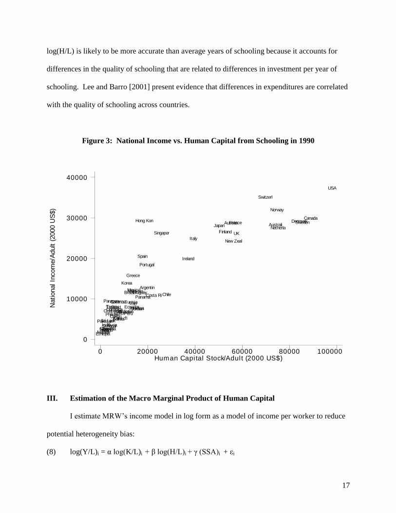
The relationship between log(H/L) with this new data and average schooling attainment

is shown in Appendix IV. While these two measures of human capital are highly correlated,

10

Financial depreciation rates for physical capital have a geometric pattern because the income generated by

physical capital does not rise over time.

11

Hong Kong’s national income is somewhat of an outlier relative to its level of human capital, no doubt due to its

unique capability in 1990 to benefit financially from its relationship to China.

17

log(H/L) is likely to be more accurate than average years of schooling because it accounts for

differences in the quality of schooling that are related to differences in investment per year of

schooling. Lee and Barro [2001] present evidence that differences in expenditures are correlated

with the quality of schooling across countries.

Figure 3: National Income vs. Human Capital from Schooling in 1990

National In

com

e/A

dult (

2000 U

S$)

Human Capi tal Stock/Adul t (2000 US$)0 20000 40000 60000 80000 100000

0

10000

20000

30000

40000

Argentin

AustraliAustria

Bolivia

Brazil

Canada

Chile

Colombia

Congo

Costa Ri

Cote d'I

Denmark

DominicaEcuador

EgyptEl Salva

Ethiopia

Finland

France

Ghana

Greece

Guatemal

Hong Kon

India

Iran

Ireland

Italy

Jamaica

Japan

Jordan

Korea

Malawi

Malaysia

Mali

Mexico

Morocco

Netherla

New Zeal

Niger

Norway

Pakistan

PanamaParaguay

PeruPhilippi

Portugal

Senegal

Singapor

Spain

Sri Lank

Sweden

Switzerl

Syria

Thailand

Togo

TunisiaTurkey

UK

Uruguay

USA

Zambia

III. Estimation of the Macro Marginal Product of Human Capital

I estimate MRW’s income model in log form as a model of income per worker to reduce

potential heterogeneity bias:

(8) log(Y/L)i = α log(K/L)i + β log(H/L)i + γ (SSA)i + εi

18

I include a dummy variable for the sub-Saharan African countries (SSA) to control for the effect

of their high morbidity and mortality rates, which reduce the effective stock of human capital in

these countries. The estimated coefficient on SSA is expected to be negative.

I use estimates per adult for Y/L, H/L, and K/L since all adults contribute directly or

indirectly to national income. I use the cumulative investment in physical capital during 1975-89

(the prior 15 years) as a proxy for the physical capital stock in each country. Since this proxy is

highly correlated with the net physical capital stock and the income model is estimated in log

form, its use does not bias the results if it is proportional to the actual stock. I estimate national

income per adult and physical capital per adult from PWT 6.2 data.12

I then add foregone

student earnings to the income data.

Even though the human capital stock is a predetermined variable, there could be reverse

causality between the stock of human capital and national income. Identifying an appropriate

instrument for human capital is difficult. Lagged values of human capital are unavailable due to

the limited historic data on investment, and they are unlikely to be valid instruments given the

lagged response of income to investments in schooling.

I use the log of the Protestant share of the population twenty years earlier (1970) as an

instrument for human capital. I obtained the Protestant share data from Barrett [1982]. The data

for log(H/L) and log(Protestant share) are shown in Figure 4. The correlation coefficient

between these variables is 0.42. Protestant affiliation is an attractive instrument for human

capital in some respects. Most countries have some level of affiliation, and the level of

affiliation has been correlated with levels of literacy and schooling across and within countries

for centuries [Cipolla, 1969, Johansson, 1981, Soysal and Strang, 1989, Goldin and Katz,

12

The data in PWT 6.2 are benchmarked to 1996 data, which provide a good basis for an analysis in 1990.

19

1998].13

Given the stability of Protestant affiliation over time, it is not an endogenous variable in

an income model.

Figure 4: Human Capital/Adult vs. Protestant Share of the Population

Log(H

um

an C

apital/A

dult)

in 1

990

Log(Protestant Share of Population) in 1970-10 -8 -6 -4 -2 0

6

7

8

9

10

11

12

Argentin

Australi

Austria

Bolivia

Brazil

Canada

Chile

ColombiaCongo

Costa Ri

Cote d'I

Denmark

Dominica

Ecuador

Egypt

El Salva

Ethiopia

FinlandFrance

Ghana

Greece

Guatemal

Hong Kon

India

Iran

IrelandItaly

Jamaica

Japan

Jordan

Korea

Malawi

Malaysia

Mali

Mexico

Morocco

Netherla

New Zeal

Niger

Norway

Pakistan

Panama

Paraguay

Peru

Philippi

Portugal

Senegal

Singapor

Spain

Sri Lank

Sweden

Switzerl

SyriaThailand

Togo

Tunisia

Turkey

UK

Uruguay

USA

Zambia

The disadvantage of Protestant affiliation as an instrument is that it could affect a nation’s

income through mechanisms not related to investment in schooling. As is well known, Weber

[1905] argued that the “Protestant ethic” causes Protestants to save more of their incomes and

13

There has long been a hypothesis that the rise of capitalism is related to the Protestants’ promotion of literacy and

education to facilitate the study of the Bible [Means, 1966 and Craig, 1981].

20

work harder. What is not well known is that Weber’s hypothesis has been overwhelmingly

rejected by the empirical evidence [Iannaccone, 1998].14

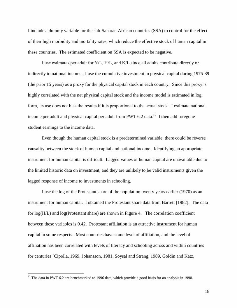
The regression results for the MRW model are shown in Table 1. Column 1 shows the

results for an OLS regression. The estimate of α in this regression (0.38) is consistent with

Bernanke and Gurkaynak’s [2001] estimate that physical capital’s share of national income is

about 35 percent across countries. The coefficients on the capital variables are highly

statistically significant, and the model accounts for 95 percent of the variation in log(Y/L) across

the 61 countries.

Table 1

Effect of Human Capital from Schooling on National Income

[Dependent Variable is Log(National Income/Adult)]

1 2 3 4 5 6

Technique OLS OLS 2SLS OLS OLS 2SLS

Countries 61 61 61 61 57 57

Log(K/L) 0.38*

(.06)

0.39*

(.06)

0.34

(.14)

0.34

(.14)

0.38*

(.07)

0.32

(.16)

Log(H/L) 0.31*

(.06)

0.30*

(.06)

0.36

(.15)

0.30*

(.06)

0.31*

(.06)

0.39

(.18)

Est Log(H/L) 0.06

(.16)

Sub-Saharan Africa -0.28*

(.11)

-0.29*

(.11)

-0.29*

(.11)

-0.29*

(.11)

-0.28*

(.11)

-0.28*

(.11)

Log(Protestant Share) 0.01

(.02)

R2 .95 .95 .95 .95 .95 .94

Note: White-adjusted standard errors in parentheses

*Significant at one percent level

14

In a recent test of Weber’s hypothesis, Becker and Wössmann [2009] show that in 453 counties in Prussia in 1871,

incomes were higher in Protestant than in Catholic counties, but that after controlling for the effect of literacy, there

is no significant difference in economic success between Protestant and Catholic counties.

21

Column 2 presents the OLS estimates with the addition of the Protestant share variable to

investigate whether Protestant affiliation affects national income directly. The direct effect of

the Protestant share on national income is negligible, the estimated coefficients on the physical

capital and human capital variables are virtually unchanged, and the variation in national income

explained by the model is unchanged. There is no indication that Protestant affiliation affects

national income other than through its effect on investment in schooling.

Column 3 presents the 2SLS estimate of the model. The coefficients on physical capital

and human capital are similar to the OLS estimate, although the estimate of β is larger. The

Hausman test in column 4 indicates that the difference between the OLS and 2SLS estimates of β

is not statistically significant. The results from the first stage of the 2SLS estimate indicate that

the Protestant share variable is a valid instrument for human capital from schooling:

(9) log(H/L) = 0.78 log(K/L) + 0.10 log(Prot Share) – 0.14 SSAfrica + 2.09 R2 = .85

(.07) (.03) (.23) (0.79)

It is possible that both the OLS and the 2SLS estimates of β are biased upward if the OLS

estimate exhibits simultaneity bias and the 2SLS estimate is biased upward due to the higher

income in the countries with a high Protestant share of the population. Columns 5 and 6 present

estimates of the model when the countries with a Protestant share of the population greater than

60 percent are excluded from the data set. This restriction eliminates four countries, leaving a

sample of 57 countries and reducing the correlation between log(H/L) and log(Prot Share) from

0.42 to 0.30 in the remaining sample. The OLS estimate of β in this subsample is identical to the

estimate in the original sample. The 2SLS estimate of β in this subsample is higher than in the

original sample and statistically significant at a three percent level of confidence. There is no

evidence that the four countries with very high levels of Protestant affiliation are driving the

2SLS estimate of the value of β in the larger sample of countries.

22

It is possible that the estimates of α and β are biased if relevant explanatory variables are

omitted from the income model. The very high R2 provides some confidence that no important

variables are missing, but conceivably these omitted factors could be highly correlated with the

two capital factors. This possibility is examined in Appendix III. The results provide evidence

that no important factors are missing and that the estimates of α and β are robust to the inclusion

of other variables in the model.

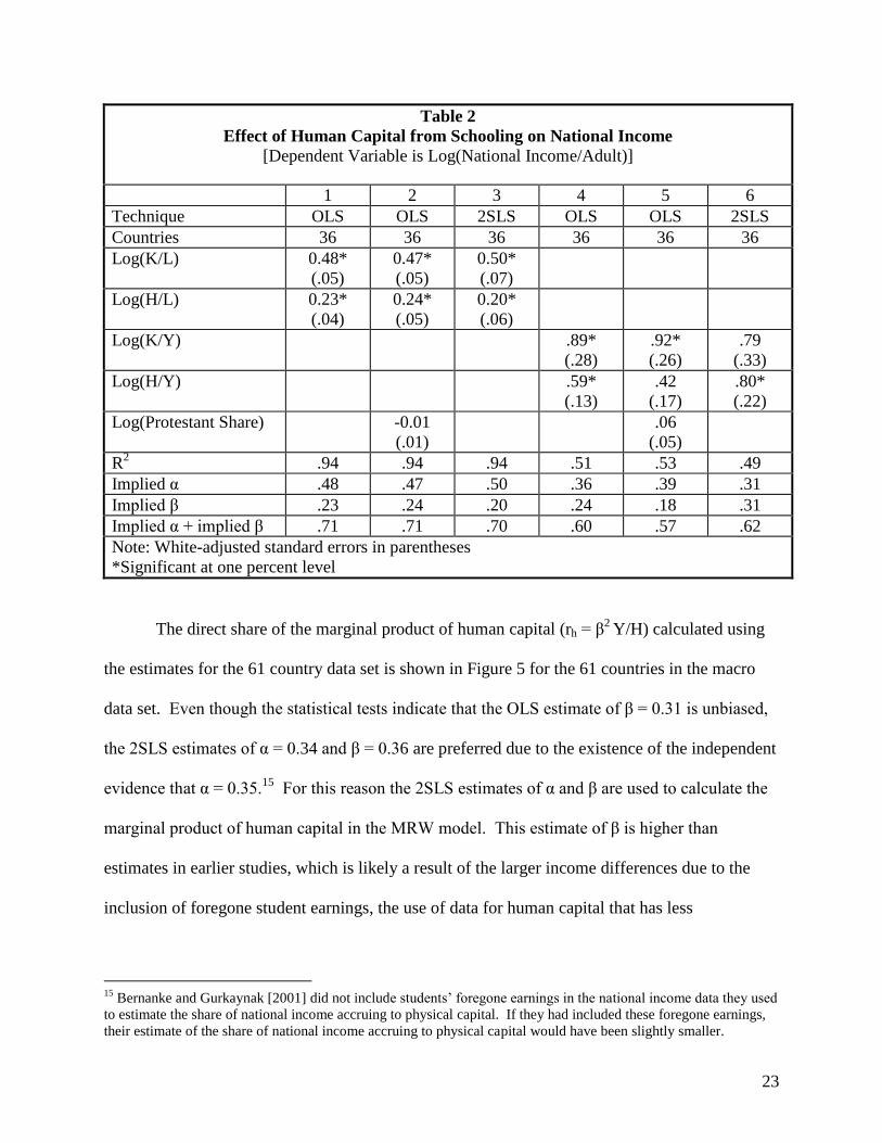
Even though the estimates of α and β are likely to be more accurate with a larger cross-

country data set, the use of 61 countries to create the macro estimates rather than the 36 countries

used for the micro estimates raises the possibility that the larger sample is not representative of

the countries to be compared. Table 2 presents estimates of the MRW model using only the 36

countries to be compared. Columns 1 to 3 show the results for the MRW model in its basic form.

In these results the estimates of α are unacceptably high (0.48 - 0.50), and the estimates of β

(0.20 - 0.23) are lower than in the larger set of countries. One possible explanation for these

results is the high correlation (ρ = 0.91) between K/L and H/L in these data.

Columns 4-6 present the estimates for a common reduced form of the MRW model.

These estimates of the effect of physical capital and human capital are more similar to the results

with the larger data set. The estimates of the effect of physical capital are lower due to bias, as is

expected when the model is estimated with K/Y instead of K/L [Cohen and Soto, 2007]. In the

2SLS estimates implied α = 0.31 and implied β = 0.31, the sum of whose values (.62) is about

11% lower than their sum (.70) in the direct form of the model. This test provides confirmation

that the estimates of α and β in the 61-country data set are representative of the relationship in

the 36-country data set.

23

Table 2

Effect of Human Capital from Schooling on National Income

[Dependent Variable is Log(National Income/Adult)]

1 2 3 4 5 6

Technique OLS OLS 2SLS OLS OLS 2SLS

Countries 36 36 36 36 36 36

Log(K/L) 0.48*

(.05)

0.47*

(.05)

0.50*

(.07)

Log(H/L) 0.23*

(.04)

0.24*

(.05)

0.20*

(.06)

Log(K/Y) .89*

(.28)

.92*

(.26)

.79

(.33)

Log(H/Y) .59*

(.13)

.42

(.17)

.80*

(.22)

Log(Protestant Share) -0.01

(.01)

.06

(.05)

R2 .94 .94 .94 .51 .53 .49

Implied α .48 .47 .50 .36 .39 .31

Implied β .23 .24 .20 .24 .18 .31

Implied α + implied β .71 .71 .70 .60 .57 .62

Note: White-adjusted standard errors in parentheses

*Significant at one percent level

The direct share of the marginal product of human capital (rh = β2

Y/H) calculated using

the estimates for the 61 country data set is shown in Figure 5 for the 61 countries in the macro

data set. Even though the statistical tests indicate that the OLS estimate of β = 0.31 is unbiased,

the 2SLS estimates of α = 0.34 and β = 0.36 are preferred due to the existence of the independent

evidence that α = 0.35.15

For this reason the 2SLS estimates of α and β are used to calculate the

marginal product of human capital in the MRW model. This estimate of β is higher than

estimates in earlier studies, which is likely a result of the larger income differences due to the

inclusion of foregone student earnings, the use of data for human capital that has less

15

Bernanke and Gurkaynak [2001] did not include students’ foregone earnings in the national income data they used

to estimate the share of national income accruing to physical capital. If they had included these foregone earnings,

their estimate of the share of national income accruing to physical capital would have been slightly smaller.

24

measurement error than the data used in other studies, and the use of the human capital stock

rather than the H/Y ratio in the model.

The rates overall exhibit a clear pattern of diminishing returns, which is particularly

pronounced for countries with very little human capital. The variation in these rates is higher

across countries with net human capital below $30,000/adult (2000$), which could be due to

greater measurement error in the data for these countries.

Figure 5: Direct Share of Macro Marginal Product of Human Capital - 1990

Direct

Share

of

Marg

inal P

roduct

of

Hum

an C

apital (%

)

Human Capi tal /Adult (2000 US$)0 20000 40000 60000 80000 100000

0

5

10

15

20

25

30

Argentin

Australi

Austria

Bolivia

Brazil

CanadaChile

Colombia

Congo

Costa Ri

Cote d'I

Denmark

Dominica

Ecuador

Egypt

El Salva

Ethiopia

FinlandFrance

Ghana

Greece

Guatemal

Hong Kon

India

Iran

Ireland

Italy

JamaicaJapan

Jordan

Korea

Malawi

Malaysia

MaliMexico

Morocco

NetherlaNew Zeal

Niger

Norway

Pakistan

Panama

Paraguay

Peru

Philippi

Portugal

Senegal

Singapor

Spain

Sri Lank

Sweden

Switzerl

Syria

Thailand

Togo

Tunisia

Turkey

UK

Uruguay

USA

Zambia

IV. Rates of Return in Workers’ Earnings Studies

Psacharopoulos and Patrinos [2004] summarize the rates of return on investment in

schooling from national workers’ earnings studies. They include “full return” private rates and

25

social rates for all levels of schooling during the period 1986-1994 for 17 of the 61 countries

included in the macro data set. I use the social rates of return in this analysis because these rates

include the public expenditures on schooling. These rates exhibit considerable variation by level

of schooling within countries and at the same level of schooling across countries. These rates

and the weighted average rate, which are actually the marginal products of schooling, are shown

in Table 3.

Table 3

Rates of Return on Investment from Earnings Studies – Full Return Method

Country Year Rate of Return (%) Share of Investment Rate (%)

Primary Second Higher Primary Second Tertiary Average

Argentina 1989 8.4 7.1 7.6 0.50 0.33 0.17 7.8

Bolivia 1990 13 6.0 13.0 0.36 0.41 0.23 10.1

Brazil 1989 35.6 5.1 21.4 0.49 0.32 0.19 23.1

Chile 1993 8.1 11.1 14.0 0.41 0.44 0.15 10.3

Colombia 1989 20 11.4 14.0 0.52 0.27 0.21 16.4

Costa Rica 1989 11.2 14.4 9.0 0.44 0.20 0.36 11.0

Ecuador 1989 14.7 12.7 9.9 0.38 0.33 0.30 12.6

El Salvador 1990 16.4 13.1 8.0 0.47 0.27 0.26 13.3

Jamaica 1989 17.7 7.9 7.9 0.54 0.37 0.08 13.2

Mexico 1992 11.8 14.6 11.1 0.52 0.24 0.24 12.3

New Zealand 1991 12.4* 12.4 9.5 0.45 0.41 0.15 12.0

Paraguay 1990 20.3 12.7 10.8 0.56 0.26 0.18 16.6

Philippines 1988 13.3 8.9 10.5 0.42 0.36 0.22 11.1

Spain 1991 7.4 8.5 13.5 0.62 0.29 0.09 8.3

UK 1986 8.6 7.5 6.5 0.40 0.49 0.10 7.8

Uruguay 1989 21.6 8.1 10.3 0.49 0.29 0.21 15.2

USA 1987 10.0* 10.0 12.0 0.37 0.43 0.20 10.4

*Unavailable rate for the primary level assumed to be the same as the rate at the secondary level.

Psacharopoulos and Patrinos [2004] summarize the Mincerian rates for 35 of the 61

countries included in the macro data set. In this data set the rates for Japan and Italy are outliers,

in that Japan is unusually high (13.2%) and Italy is unusually low (2.7%). I investigated the

sources for these rates and found that the rates are incorrect. Cohn and Addison’s [1998] rates

26

for Japan are a range of 4.4% to 13.2%, so I used the midpoint of 8.8%. Brunello and Miniaci’s

[1999] rate for Italy is 5.6%.

Of the 36 countries that had either a full return rate or a Mincerian rate, 16 countries had

both rates. Two countries, Brazil and Jamaica, have pairs of rates that are outliers. Excluding

these two countries, the remaining 14 countries have an average full rate of return (i.e., a

marginal product) that is 1.19 times the average Mincerian rate. I use this factor to estimate the

marginal product of schooling for the 19 countries that had only a Mincerian rate.

The resulting set of micro rates (actually marginal products of schooling) is shown in

Figure 6 and is provided in Appendix II. While there is a clear pattern of diminishing returns,

Figure 6: Rates of Return on Investment in Schooling from Earnings Studies - 1990

Rate

of

Retu

rn o

n I

nvestm

ent

in S

choolin

g (

%)

Human Capi tal /Adult (2000 US$)0 20000 40000 60000 80000 100000

0

5

10

15

20

25

Argentin

Australi

Austria

Bolivia

Brazil

CanadaChile

Colombia

Costa Ri

Denmark

Dominica

EcuadorEl Salva

FinlandGreece

Guatemal

Italy

Jamaica

Japan

Korea

Mexico

Netherla

New Zeal

Pakistan

PanamaParaguay

Peru

Philippi

Portugal

Spain

Sweden

Switzerl

Thailand

UK

Uruguay

USA

27

there is also considerable variation in these rates. This variation is likely due in part to

measurement error in the data on workers’ earnings and school expenditures, and especially in

the estimates of students’ foregone earnings, which, as shown in Appendix I, can vary

considerably between micro studies due to differences in estimation methodologies.

V. Comparison of Macro and Micro Marginal Products

Table 3 provides a summary of the estimates of the micro and macro marginal products

data for the 36 countries that had both rates. The average direct share of the marginal product of

human capital in the MRW model was 9.8 percent, while the average micro marginal product of

schooling was 11.6 percent. The correlation coefficient between these two sets of rates is 0.57.

A student’s t test indicates that the two data samples are correlated with a level of significance

above one percent.

The two sets of rates are not entirely comparable because the workers’ level of

experience is not the same in the two data sets. Due to the growth in the world population over

the 1930-1970 period, the 1990 worldwide work force in the macro analysis had about 2.5 years

less experience than it would have had in the absence of population growth.

Table 4

Summary Characteristics for Micro and Direct Macro Rate-of-Return Data

Variable Obs. Mean Std. Dev. Minimum Maximum

Micro – Earnings studies 36 11.6 3.9 5.4 23.1

Macro – Direct – Low Experience 36 9.8 5.6 4.3 26.6

Macro – Direct adjusted 36 10.7 6.1 4.7 29.2

Macro – Direct (adj) + External 36 19.6 11.2 8.6 53.4

The earnings patterns in Figure 2 combined with the 1990 distribution of schooling by

level in Cohen and Soto [2007] indicate that a 2.5-year reduction in average experience (12.5

28

percent of 20 years) is likely to have reduced the aggregate earnings of the workers in the macro

study by about six percent relative to workers with an average level of experience. Adjusting

national income upward in each country to offset this decline in the average experience of the

work force raises the mean of the direct macro rates to 10.7 percent. The associated adjusted

macro rates that include the external effect of schooling on the labor wage (w) are also shown in

the table. These rates are a 1.83 multiple ((1-α)/β) of the adjusted direct macro rates. The mean

of these rates is 19.6 percent.

The mean of the micro rates is 12 percent greater than the mean of the direct adjusted

macro rates and 41 percent less than the mean of the direct + external adjusted macro rates. So

the mean of the micro rates is consistent with the means of the adjusted macro rates, but the

consistency of the means does not ensure that the two sets of rates are consistent across countries

with different levels of human capital.

Figure 7 shows the individual estimates of the micro rates for the 36 countries and the

fitted trend for these estimates, ordered by the national level of (net) human capital from

schooling. The figure also shows the fitted trend for the direct share of the adjusted macro rates

(i.e., the share that accrues directly to the recipient of schooling) and the fitted trend for the direct

share plus the external share of the adjusted macro rates that accrues to labor for the same 36

countries. Given the considerable variation in individual micro and macro rates, the trends in the

data are more meaningful than the individual rates.

Both the micro and the macro rates exhibit diminishing returns, but the relationship

between these rates is quite different over the range of countries. In the countries with low levels

of human capital from schooling, the trend for the micro rates tracks the trend for the direct share

of the macro rates. As the level of human capital from schooling rises, the trend for the micro

29

rates rises above the trend for the direct share of the macro rates. For the countries with the

highest level of human capital, the micro trend approaches the trend for the macro rates that

include the sum of the direct share and the external share that accrues to labor.

Figure 7: Macro and Micro Marginal Products of Schooling

0

5

10

15

20

25

30

35

40

0 20000 40000 60000 80000 100000

Marg

inal P

rocd

uct (%

)

Human Capital/Adult (2000 US$)

Micro Estimates Macro Direct Trend

Micro Trend Macro Direct + External Trend

The implication of the pattern of rates in Figure 7 is that in countries with low levels of

human capital, the external marginal product of schooling in 1990 accrued equally to the entire

work force, so it did not affect the micro estimates of the marginal product of schooling. In

countries with human capital from schooling of $100,000/adult, the external marginal product of

schooling accrued to the more schooled workers, so the effect is included in the micro estimates

of the marginal product of schooling.

30

How robust are these trends in the rates? The trend for the micro rates is quite robust,

with a trend that is unlikely to exhibit much measurement error. Psacharopoulos and Patrinos

[2004] present many estimates of rates of return on investment in schooling for more recent

years in many countries, and they are consistent with these rates.

The trends in the macro rates are based on the upper bound MPH = (1-α)β Y/H and the

lower bound MPH = β2 Y/H. The value of α is approximately 0.35 in all valid estimates of the

MRW model, so it is stable. Since there are only two variables in the model, K/L and H/L,

which are similar in magnitude and highly correlated with Y/L, the sum α + β is extremely stable.

As shown in Table 2, when the model is estimated as a function of K/Y, this (biased) sum tends

to be 0.6, as it is in MRW’s original estimates. The sum of the unbiased estimates is expected to

be higher, closer to 0.7, as shown in Table 1. As a result, if α = 0.35, β must be approximately

0.35 as well.

In the current estimation of β in the MRW model, the econometric results are unaffected

by the ratio of foregone earnings to direct expenditures because this ratio is constant across

countries and the MRW model is estimated in log form. But this ratio does affect the estimate of

H in the macro rates, so this is where the macro rates may encounter uncertainty. In the

reconciliation this ratio is assumed to be 1.9 for all countries, but the data shown in Appendix I

indicate that this ratio conceivably could be as low as 1.7 and as high as 2.1. This variation

would change the macro rates by +/ 1% at the upper bound and +/- 0.5% at the lower bound.

Variations of this order of magnitude in the macro marginal products would not invalidate the

results of the reconciliation exercise. The micro and macro rates would still be consistent.

Even in countries with human capital/adult of $100,000/adult, not all of the marginal

external effect of schooling in 1990 was captured by schooled workers, since the α share of the

31

marginal product in the macro rates of return does not accrue to the work force. As a result, the

nation’s marginal product of human capital substantially exceeds the marginal product of

schooling in workers’ earnings studies in all countries. This external marginal product, the

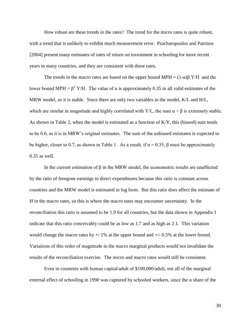
difference between the macro and micro marginal products, is shown in Figure 8. The external

marginal product in 1990 was about 2/3 of the market rate (actually marginal product of

schooling) in countries with high levels of human capital, but it was substantially above the

market rate in countries with low levels of human capital.

Figure 8: Market and External Marginal Products of Schooling

0

10

20

30

40

50

60

0 20000 40000 60000 80000 100000

Marg

inal P

rod

uct (%

)

Human Capital/Adult (2000$)

External Estimates External Trend Market Trend

The empirical results indicate that the decline in the marginal product of human capital

due to diminishing returns is relatively slow. With the increase in the net human capital stock

from $50,000/adult to $100,000/adult (2000 US$), the market rate in 1990 declined from about

32

10 percent to about 8.5 percent, while the total marginal product, including the external effects,

declined from about 18 percent to about 14 percent.

The external marginal product includes the marginal product that accrues to physical

capital and to labor. The external marginal product to labor alone, the difference between the

share of the marginal product accruing to workers and the micro marginal product, is not shown

in Figure 8. As can be inferred from the relationship in Figure 7, this rate was high in countries

with little human capital in 1990 but diminished to a very low rate in countries with (net) human

capital from schooling greater than $90,000/adult (2000 US$).

Empirical studies of the external effect of human capital on physical capital and labor

within countries are consistent with the results in Figures 7 and 8. Chi [2008] and Lopez-Bazo

and Moreno [2008] present evidence that historically an increase in human capital raised

investment in physical capital in China and Spain. Acemoglu and Angrist [2001] and Moretti

[2004] present evidence that human capital has a small external effect on workers’ salaries in the

U.S. Liu [2007] and Fleisher, Li, and Zhao [2010] present evidence that human capital has a

large external effect on workers’ salaries in China.

VI. Conclusions

This paper presents the results of a test to determine whether Mankiw, Romer, and Weil’s

model of economic growth has a marginal product of human capital that is consistent with the

estimates of the return on investment in schooling in micro studies. In the MRW model human

capital has two external effects, one on physical capital and one on labor. Since workers receive

income from human capital through the direct effect (β) and through the external or spill-over

effect (1-α-β) on labor, their total income is bounded by the direct effect on the low side and the

sum of these two effects on the high side. If the MRW model is valid, the independent estimates

33

of the increase in workers’ incomes that accompanies increased schooling should fall within

these bounds.

After estimating the MRW model with a new set of human capital and national income

data, I show that across 36 countries the fitted trends for the macro estimates of the marginal

product of human capital in 1990 are consistent with the fitted trend for the micro estimates. In

this comparison the relationship between the micro and macro rates follows a well-defined

pattern. In the lowest-income countries, the micro rate is equal to the direct share of the macro

marginal product (i.e., the β share). The share accruing to workers increases as countries

increase their level of human capital until in the highest-income countries, the micro rate is

almost equal to the direct share plus the external share of the marginal product that accrues to

labor (i.e., the 1-α share). These results indicate that in 1990 as the stock of human capital

increased, a higher share of the external returns from schooling accrued to the more educated

component of the work force. The results indicate that physical capital and skill are

complementary at all levels of human capital. They indicate that human capital and unschooled

labor are also complementary, but the marginal effect of human capital on the marginal product

of labor is small at high levels of human capital.

The empirical results in this analysis provide evidence that MRW’s growth model is a

valid representation of the growth process. The results also provide evidence that investment in

human capital has large external effects on national income and that these effects are larger in

countries with lower levels of human capital.

34

REFERENCES

Acemoglu, Daron, and Johnson, Simon, 2007, “Disease and Development: The Effect of Life

Expectancy on Economic Growth,” Journal of Political Economy, v115, n6, 925-985

Acemoglu, Daron, and Angrist, Joshua, 2001, “How large are human capital externalities?

Evidence from Compulsory Schooling Laws,” NBER Macroeconomics Annual 2000, MIT Press,

9-59

Breton, Theodore R., 2010, “Schooling and National Income: How Large are the Externalities?”

Education Economics, v18, n1, 67-92

Barrett, David B., 1982, The World Christian Encyclopedia, Oxford University Press, New York

Barro, Robert J., and Lee, Jong-Wha, 2001, “International data on educational attainment:

updates and implications, Oxford Economic Papers 3, 541-563

Becker, Sascha O., and Wössmann, Ludger, 2009, “Was Weber Wrong? A Human capital

Theory of Protestant Economic History,” Quarterly Journal of Economics, v124, i2, 531-596

Bernanke, Ben S., and Gurkaynak, Refet S., 2001, “Taking Mankiw, Romer, and Weil

Seriously,” NBER Macroeconomics Annual, v16, 11-57

Brunello, Giorgio, and Miniaci, Raffaele, 1999, “The Economic Returns to Schooling for Italian

Men. An Evaluation Based on Instrumental Variables,” Labour Economics, v6, 509-519

Caselli, Francesco, and Feyrer, James, 2007, “The Marginal Product of Capital,” Quarterly

Journal of Economics, v122, n2, 535-568

Chi, Wei, 2008, “The Role of Human Capital in China’s Economic Development: Review and

New Evidence,” China Economic Review, v19, 421-436

Ciccone, Antonio, and Jarocinski, Marek, 2010, “Determinants of Economic Growth: Will Data

Tell? American Economics Journal: Macroeconomics v2, n4, 222-246

35

Cipolla, Carlo M., 1969, Literacy and Development in the West, Pelican Books, Baltimore

Cohen, Daniel, and Soto, Marcelo, 2007, “Growth and Human Capital: Good Data, Good

Results,” Journal of Economic Growth, v12, n1, 51-76

Cohn, Elchanan, and Addison, John T., 1998, “The Economic Returns to Lifelong Learning in

OECD Countries,” Education Economics, v6, n3, 253-306

Craig, John E., 1981, “The Expansion of Education,” Review of Research in Education, v9, 151-

213

Fleisher, Belton, Li, Haizheng, and Zhao, Min Qiang, 2010, “Human Capital, Economic Growth,

and Regional Inequality in China,” Journal of Development Economics, v92, 215-231

Goldin, Claudia and Katz, Lawrence F., 1998, “Human Capital and Social Capital: The Rise of

Secondary Schooling in America, 1910 to 1940,” Working Paper 6439, National Bureau of

Economic Research, Cambridge

Gomez-Castellanos, Luisa, and Psacharopoulos, George, 1990, “Earnings and Education in

Ecuador: Evidence from the 1987 Household Survey,” Economics of Education Review, v9, n3,

219-227

Hall, Robert E., and Jones, Charles I., 1999, Why Do Some Countries Produce So Much More

Output Per Worker Than Others?” Quarterly Journal of Economics, v114, n1, 83-116

Heston, Alan, Summers, Robert, and Aten, Bettina, 2006, Penn World Table Version 6.2, Center

for International Comparisons of Production, Income and Prices at the University of

Pennsylvania (CICUP), September

Hossain, Shaikh I., and Psacharopoulos, George, 1994, “The Profitability of School Investments

in an Educationally Advanced Developing Country,” International Journal of Educational

Development, v14, n1, 35-42

36

Iannaccone, Laurence R., 1998, “Introduction to the Economics of Religion,” Journal of

Economic Literature 36, 1465-1496

Johansson, Egil, 1981, “The History of Literacy in Sweden,” in Graff, Harvey J., Literacy and

Social Development in the West: A Reader, Cambridge University Press, New York, 151-182

Kendrick, John W., 1976, The Formation and Stocks of Total Capital, National Bureau of

Economic Research, New York

Klenow, Peter J., and Rodriguez-Clare, Andres, 1997, “The Neoclassical Revival in Growth

Economics: Has It Gone Too Far?” NBER Macroeconomics Annual, v12, 73-103

Lee, Jong-Wha, and Barro, Robert J., 2001, “Schooling Quality in a Cross-Section of Countries,”

Economica 68, 465-488

Levine, Ross, and Renelt, David, 1992, “A Sensitivity Analysis of Cross-Country Growth

Regressions,” The American Economic Review, v82, i4, 942-963

Liu, Zhiqiang, 2007, “The External Returns to Education: Evidence from Chinese Cities,”

Journal of Urban Economics, v61, n3, 542-564

Lopez-Bazo, Enrique, y Moreno, Rosina, 2008, “Does Human Capital Stimulate Investment in

Physical Capital? Evicence from a Cost System Framework,” Economic Modelling v25, 1295-

1305

Mankiw, N. Gregory, Romer, David, and Weil, David N., 1992, “A Contribution to the Empirics

of Economic Growth,” Quarterly Journal of Economics, v107, Issue 2, 407-437

Mauro, Paolo, 1995, “Corruption and Growth,” Quarterly Journal of Economics, v110, n3, 681-

712

Means, Richard L., 1966, “Protestantism and Economic Institutions: Auxiliary Theories to

Weber’s Protestant Ethic,” Social Forces, v44, n3, 372-381

37

Mirestean, Alin, and Tsangarides, Charalambos, 2009, “Growth Determinants Revisited,” IMF

Working Paper WP/09/268

Moretti, Enrico, 2004, “Estimating the social return to higher education: evidence from

longitudinal and repeated cross-sectional data,” Journal of Econometrics, 121, 175-212

OECD, 2001, “Measuring Capital; OECD Manual: Measurement of Capital Stocks,

Consumption of Fixed Capital, and Capital Services,” OECD Publication Services,

www.SourceOECD.org

Psacharopoulos, George, 1973, Returns to Education: An International Comparison, Jossey-Bass

Inc., Publishers, San Francisco

Psacharopoulos, George and Patrinos, Harry, 2004, “Returns to Investment in Education: A

Further Update,” Education Economics, v12, n2, 111-134

Psacharopoulos, George, and Velez, Eduardo, 1994, "Education and the Labor Market in

Uruguay," Economics of Education Review, v13, n1, 19-27

Psacharopoulos, George, Velez, Eduardo, and Patrinos, Harry Anthony, 1994, "Education and

Earnings in Paraguay," Economics of Education Review, v13, n4, 321-327

Soysal, Yasemin Nuhoglu, and Strang, David, 1989, “Construction of the First Mass Education

Systems in Nineteenth-Century Europe, Sociology of Education, v62, n4, 277-288

Tilak, Jandhyala B. G., 1988, “Costs of Education in India,” International Journal of

Educational Development, v8, n1, 25-42

Weber, Max, 2000 (1905), The Protestant Ethic and the Spirit of Capitalism, Routledge, New

York

38

Appendix I

Ratio of Foregone Earnings to National Expenditures on Schooling

I estimated the ratio of foregone earnings to cumulative national expenditures on

schooling in 1990 using data from studies in nine countries. The data came from several sources.

I obtained raw data on direct costs and foregone earnings by level of schooling in the late 1960s

for nine countries from Psacharopoulos [1973]. I weighted these data using the 1970 distribution

of schooling by level provided in Cohen and Soto [2007] and an assumed schooling duration of

six years for primary and secondary schooling and four years for university. The resulting

estimates of the ratio of foregone earnings to direct expenditures are shown in Table A-1. These

estimates range from 0.23 in Malaysia to 1.54 in Great Britain. The average ratio is 1.02. The

enormous variation in these estimates is not a function of the level of national income.

Table A-1

Ratios of Foregone Earnings to Direct Schooling Costs

Estimated* Tilak [1988] Kendrick [1976]

Chile 0.69

Colombia 0.79

India 1.12 0.86

South Korea 1.27

Malaysia 0.23

Mexico 1.53

Great Britain 1.54

New Zealand 1.03

United States 0.99 0.90

Average 1.02

*Estimated from data on direct costs and foregone earnings in Psacharopoulos [1973].

Psacharopoulos’s notes reveal that in some countries the foregone earnings data are not

representative of all workers. In the U.S. the data are for white males only. In Great Britain

foregone earnings at the university level are for science and engineering students. In Colombia

workers were assumed to work full-time for 50 weeks, with no period of unemployment. These

39

differences are likely to lead to an overestimate of foregone earnings under actual working

conditions in these three countries.

Tilak [1988] provides estimates of the ratio of foregone earnings in India in 1979-80.

The upper bound on his ratio of foregone earnings to expenditures on schooling is 0.72. He also

provides Kothari’s estimates of the ratio of foregone earnings to direct expenditures in India for

1960, which averaged 0.99. Both of these estimates are below the ratio of 1.12 percent for India

calculated from the data in Psacharopoulos [1973]. The average ratio for the two comprehensive

studies in India is 0.86.

Kendrick [1976] estimated the total capital investment in the U.S. in 1969. He estimated

that the ratio of foregone earnings to direct expenditures was 0.90. This estimate also is below

the ratio of 0.99 for the U.S. calculated from the data in Psacharopoulos [1973].

Since foregone earnings are overestimated in Psacharopoulos’s data, the average ratio of

foregone earnings to direct expenditures in the nine countries is below 1.02. The average ratio in

the two comprehensive studies in India and the U.S. is 0.88. Based on this review of the data in

these studies, I estimate that that foregone earnings were approximately 90 percent of direct

expenditures in all countries.

40

Appendix II

Data Used in the Analysis

The key data used in the analysis and some of the data used to create these data are

provided in Table A-2. The national income and human capital data are in 2000 US$.

Table A-2

Data Used in the Analysis

Country Y/L H/L School

Fin Mult

Model

MPH

Labor

Growth

Adjusted

MPH

Mincer

Return

Micro

MPS

$/Adult $/Adult Ratio Percent Percent Percent Percent Percent

Argentina 12305 19766 1.39 22.4 1.6 24.6 10.3 7.8

Australia 27834 74055 1.58 13.5 2.0 14.8 8.0 9.5

Austria 28286 55069 1.49 18.5 0.4 20.3 7.2 8.6

Bolivia 4561 7637 1.34 21.5 2.2 23.6 10.7 10.1

Brazil 11096 12214 1.33 32.7 2.9 35.8 14.7 23.1

Canada 29461 88933 1.55 11.9 2.1 13.1 8.9 10.6

Chile 10622 28037 1.40 13.6 2.2 14.9 12.0 10.3

Colombia 8793 7610 1.34 41.6 2.9 45.6 14.0 16.4

Congo-Rep 5163 6437 1.32 28.9

Costa Rica 10400 22667 1.33 16.5 3.3 18.1 8.5 11.0

Cote d`Ivoire 4739 8565 1.32 19.9 3.9

Denmark 28730 84260 1.53 12.3 0.8 13.5 4.5 5.4

Dominican Rep 6921 6034 1.33 41.3 3.0 45.3 9.4 11.2

Ecuador 7528 13352 1.35 20.3 2.9 22.2 11.8 12.6

Egypt 6033 8081 1.31 26.9

El Salvador 6418 10845 1.32 21.3 2.5 23.4 7.6 13.3

Ethiopia 896 1036 1.32 31.1

Finland 26090 52791 1.44 17.8 0.9 19.5 8.2 9.8

France 28326 57044 1.44 17.9

Ghana 2143 2159 1.32 35.7

Greece 15288 13792 1.39 39.9 1.0 43.7 7.6 9.0

Guatemala 6522 5154 1.31 45.6 3.0 49.9 14.9 17.7

Hong Kong 28855 18620 1.37 55.8

India 3112 2413 1.32 46.4

Iran 8375 13910 1.32 21.7

Ireland 19460 37106 1.44 18.9

Italy 24425 39449 1.39 22.3 0.8 24.4 5.6 6.7

Jamaica 7250 15293 1.37 17.1 1.5 18.7 28.8 13.2

Japan 27617 50190 1.55 19.8 1.6 21.7 8.8 10.5

Jordan 7088 15669 1.35 16.3

Korea, Rep 13451 11150 1.40 43.4 2.7 47.6 13.5 16.1

Malawi 1323 1174 1.32 40.6

41

Malaysia 11431 14827 1.34 27.8

Mali 1703 1900 1.32 32.3

Mexico 11731 14052 1.35 30.1 2.9 32.9 7.6 12.3

Morocco 6366 9977 1.32 23.0

Netherlands 27099 75178 1.50 13.0 1.4 14.2 6.4 7.6

New Zealand 23822 56321 1.52 15.2 1.7 16.7 10.3 12.0

Niger 2019 1755 1.32 41.4

Norway 31529 74667 1.54 15.2

Pakistan 3998 1944 1.31 74.0 2.4 81.1 15.4 18.3

Panama 9998 17969 1.35 20.0 2.7 22.0 13.7 16.3

Paraguay 8981 4904 1.34 65.9 2.5 72.3 11.5 16.6

Peru 5919 11853 1.35 18.0 2.8 19.7 8.1 9.6

Philippines 5652 4705 1.35 43.3 2.9 47.4 11.1

Portugal 17942 19729 1.33 32.7 0.7 35.9 8.6 10.2

Senegal 2823 3629 1.32 28.0

Singapore 25801 25985 1.37 35.7

Spain 20032 17803 1.39 40.5 1.1 44.4 7.2 8.3

Sri Lanka 4152 3306 1.34 45.2

Sweden 28411 85441 1.53 12.0 0.7 13.1 5.0 6.0

Switzerland 34665 69732 1.63 17.9 1.2 19.6 7.5 8.9

Syria 3039 5067 1.32 21.6

Thailand 7413 5504 1.32 48.5 3.0 53.1 11.5 13.7

Togo 1804 3333 1.32 19.5

Tunisia 8756 12898 1.31 24.4

Turkey 7604 5063 1.32 54.1

UK 25680 57567 1.54 16.1 0.4 17.6 6.8 7.8

Uruguay 11112 16636 1.37 24.0 0.9 26.4 9.7 15.2

USA 36912 98073 1.60 13.5 1.4 14.9 10.0 10.4

Zambia 2132 3573 1.33 21.5

42

Appendix III

Omitted Variables Analysis

Hundreds of cross-country studies have tried to determine which factors affect economic

growth. Levine and Renelt [1992] examined over 50 variables that had been shown to be

correlated with economic growth and showed that few are robust to changes in the

accompanying set of variables in the growth model. Since then numerous researchers have used

Bayesian techniques in an effort to determine whether some variables are more robust than

others. Depending on how they structure their priors and which data sets and time periods they

analyze, they come to different conclusions. Ciccone and Jarocinski [2010] conclude that

variables purported to be robustly correlated with growth are not robust to changes in the cross-

country data sets.

One serious limitation with Ciccone and Jarocinski’s study and with the others that they

replicate is that they do not control for endogeneity bias. They attempt to limit this bias by only

selecting explanatory variables from early in the growth period, but in the process they introduce

specification error or measurement error into their analysis.16

For example, in the dynamic

version of the MRW model, the rates of investment in physical capital and human capital are the

constant (or at least the average) rates over the growth period. When the data for these variables

are taken from early in the period to minimize endogeneity bias, these variables are at least

poorly measured. As a result, when the neoclassical variables are found not to be robust, it is not

clear if this is because they are invalid or because they are mis-measured.

Mirestean and Tsangarides [2009] employ a Bayesian technique to examine whether a

large number of variables are robust, and they attempt to control for endogeneity by using lagged

16

Ciccone and Jarocinski [2010] do not address the endogeneity problem, but they replicate Sala-i-Martin,

Doppelhofer, and Miller’s [2004] analysis, who state that they chose their variables from early in the growth period

partly to deal with the endogeneity problem.

43

variables and differences in the lagged variables as instruments. As will be discussed below, it is

not clear that they succeeded in eliminating endogeneity bias in all of their estimated coefficients,

but they at least made the effort to do so, and they managed to identify some variables that

according to their methodology are robust. In this appendix I examine whether the estimates of α

and β in the MRW model are robust to the addition of these variables to the model.

Mirestean and Tsangarides performed several different analyses. Overall they found the

strongest evidence for the robustness of initial income, investment, population growth, and life

expectancy. They found less strong evidence for debt, trade openness, and inflation.

They found only weak evidence for the robustness of education, but the variable they

created for education was the average stock of primary and secondary schooling. It is not clear

why they excluded tertiary education from their variable, but its exclusion undermines the

validity of their results, since it eliminates most of the variation in education across high-income

countries. One common problem with the Bayesian analyses is that while they examine a vast

array of variables, invariably some of these variables are not ideally specified.

Three of the four most robust variables in their analysis (initial income, investment, and

population growth) are the standard neoclassical variables, which implicitly are already included

in the MRW model. This leaves debt, trade openness, inflation, and life expectancy as the four

additional variables to be tested. Inflation and debt are expected to have a negative effect, while

life expectancy and trade openness are expected to have a positive effect. The specific variables

tested are the net government debt to GDP ratio in 1990, the trade openness variable in 1990,

log(1 + the GDP deflator) for 1990 and life expectancy at birth in 1990. The data for these

variables were obtained from IMF statistics (debt), PWT 6.2, (openk), and the World Bank’s

World Development Indicators.

44

The empirical results for the model are shown in Table A-3. Column 1 shows the OLS

estimate of the MRW model. Column 2 shows the results for this model, including all of the

additional variables except debt. Debt was excluded initially because data were available in

1990 for only 32 of the 61 countries. When the three variables are included in the model, the

estimates of α and β are robust, but β is smaller (0.22 vs. 0.31) than in the standard model. The

coefficient on trade openness has the wrong sign and is not significant, but the coefficients on the

other two variables have the correct signs and are statistically significant.

Table A-3

Effect of Human Capital from Schooling on National Income

[Dependent Variable is Log(National Income/Adult)]

1 2 3 4 5 6 7 8

Technique OLS OLS OLS 2SLS 2SLS 2SLS OLS 2SLS

Countries 61 61 61 61 61 61 57 32

Log(K/L) 0.38*

(.06)

0.39*

(.06)

0.41*

(.07)

0.34

(.14)

0.33*

(.12)

0.33

(.14)

0.47*

(.15)

0.40

(.16)

Log(H/L) 0.31*

(.06)

0.22*

(.05)

0.29*

(.06)

0.36

(.15)

0.31

(.15)

0.37

(.15)

0.22

(.09)

0.32

(.13)

Sub-Saharan

Africa

-0.28*

(.11)

-0.02

(.15)

-0.28*

(.11)

-0.29*

(.11)

-0.10

(.17)

-0.29*

(.10)

-0.05

(.19)

-0.08

(.19)

Debt to GDP

Ratio

-0.42

(.39)

-0.52

(.45)

Trade Openness -0.09

(.06)

-0.06

(.07)

-0.07

(.08)

-0.04

(.09)

-0.12

(.07)

-0.10

(.07)

Inflation -0.06

(.03)

-0.08*

(.03)

-0.06

(.03)

-0.07

(.04)

-0.00

(.56)

0.23

(.58)

Life Expectancy 0.02

(.01)

0.01

(.01)

0.01

(.02)

0.01

(.02)

R2 .95 .96 .96 .95 .96 .95 .98 .98

Note: White-adjusted standard errors in parentheses *Significant at one percent level

Column 3 shows the OLS results without life expectancy, which shows that the decline in

β in column 2 is due almost entirely to the inclusion of this variable. Acemoglu and Johnson

[2007] have examined the effect of life expectancy on economic development, and they show

45

that while it reduces population growth, there is no evidence that it raises income per capita. It

seems likely that life expectancy is endogenous in this income model, since life expectancy rises

with national income. It is also highly correlated with human capital (ρ = 0.83), and

conceptually it seems more likely that higher human capital raises life expectancy rather than the

reverse.

Columns 4 to 6 show the 2SLS estimates for the same models. The estimates of α and β

continue to be robust, and in these results the magnitude of β is less affected by the inclusion of

life expectancy in the model. The estimate of β declines from 0.36 to 0.31 when the other

variables are added to the model.

Columns 7 and 8 show the results when the debt to GDP ratio is added to the model. The

estimated coefficient on debt has the expected sign, but it is not statistically significant.

Although the sample includes only 32 countries, the estimates of α and β continue to be robust.

In the 2SLS estimates, value of β declines to 0.32.

Overall in the various models the estimates of α and β are consistently positive and

statistically significant at the five percent level or higher. Only the inclusion of life expectancy

reduces the estimate of β in a non-trivial way. Acemoglu and Johnson’s [2007] evidence

indicates that life expectancy is not a determinant of economic growth, so its capability to reduce

the magnitude of β is likely to be a result of endogeneity bias. The inclusion of the other

variables in the income model have virtually no effect on the estimates of α and β in the

regressions.

46

Appendix IV

A Comparison of the Net Human Capital Stock to Average Schooling Attainment

This appendix presents the estimates of the national income model in equation (8) using

Cohen and Soto’s [2007] and Barro and Lee’s [2001] estimates of average schooling attainment.

These estimates can be compared to the estimates in Table 1 to investigate whether the data on

net human capital provide more acceptable estimates of the national income model than the

schooling attainment data. Due to differences in the countries for which data are available,

slightly fewer countries are used in these regressions than in the results shown in Table 1.

Figure A-1 shows the relationship between log(H/L) and Cohen and Soto’s [2007]

estimates of schooling attainment in the population from 15 to 64 in 1990. This relationship is

linear because investment per year of schooling rises at an increasing rate as average years of

schooling rises [Breton, 2010]. Across the countries in the data set, average years of schooling

vary by a factor of 17, while net human capital per adult varies by a factor of 100. For this

reason in the income model β log(H/L) is represented by θ Attainmentit:

(10) log(Y/L)it = α log(K/L)it + θ Attainmentit + γ (SSA)it

This log-linear relationship between income and schooling attainment is consistent with the

standard Mincerian relationship.

Table A-4 presents the results from the various estimates of the model. The 2SLS

estimates utilize the log of the Protestant share of the population as an instrument. The implied

values of β shown in the table are estimated using a conversion factor to relate the effect of

average schooling attainment to the effect of net human capital from schooling. For the Cohen

47

and Soto [2007] 1990 data, a regression indicated that log(H/L) = 0.32 Attainment, while for the

Barro and Lee [2001] 1990 data, log(Hs/L) = 0.38 Attainment.

Figure A-1: Log(Human Capital per Adult) vs. Average Schooling Attainment in 1990

Log(H

um

an C

apital p

er

Ad

ult)

Average Schooling Attainment per Adult (years)0 1 2 3 4 5 6 7 8 9 10 11 12 13

6

7

8

9

10

11

12

Argentin

Australi

Austria

Bolivia

Brazil

Canada

Chile

Colombia

Costa Ri

Cote d`I

Denmark

Dominica

Ecuador

Egypt

El Salva

Ethiopia

FinlandFrance

Ghana

Greece

Guatemal

India

Iran

IrelandItaly

Jamaica

Japan

Jordan

Korea, R

Malawi

Malaysia

Mali

Mexico

Morocco

Netherla

New Zeal

Niger

Norway

Panama

Paraguay

Peru

Philippi

Portugal

Senegal

Singapor

Spain

Sweden

Switzerl

SyriaThailand

Tunisia

Turkey

UK

Uruguay

USA

Zambia

The empirical results for the standard income model are typical of the statistical estimates

in earlier studies, which provide inconsistent estimates of α that are greater than physical

capital’s share of national income and estimates of β that are relatively small. The similarity of

the OLS and the 2SLS estimates of the effect of average attainment indicates that these

unsatisfactory estimates of α are not due to simultaneity bias.

48

Table A-4

Effect of Human Capital from Schooling on National Income

[Dependent Variable is Log(National Income/Adult)]

1 2 3 4 5 6 7 8

Cohen and Soto [2007] Data Barro and Lee [2001] Data

Technique OLS OLS 2SLS 2SLS OLS OLS 2SLS 2SLS

Countries 56 56 56 56 58 58 58 58

Log(K/L) 0.55*

(.07

0.52*

(.07)

0.58*

(.06)

0.54*

(.08)

Log(K/Y) 0.26

(.16)

0.32

(.15)

0.30

(.15)

0.32

(.14)

Average Attainment 0.05

(.02)

0.17*

(.02)

0.06

(.03)

0.15*

(.03)

0.05

(.03)

0.20*

(.02)

0.07

(.04)

0.20*

(.03)

Sub-Saharan Africa -0.18

(.19)

-0.74*

(.25)

-0.18*

(.20)

-0.81*

(.28)

-0.30

(.14)

-0.78*

(.18)

-0.29

(.15)

-0.80*

(.21)

R2 .93 .81 .93 .81 .93 .78 .93 .78

Implied α .55 .21 .52 .24 .58 .23 .54 .24

Implied β .16 .42 .19 .36 .13 .41 .21 .40

Note: White-adjusted standard errors in parentheses

*Significant at one percent level

The table also presents the results for a reduced form of the income model, in which the

model is converted to a function of the capital/output ratio (K/Y):

(11) log(Y/L)it = α/1-α log(K/Y)it + θ/1-α Attainmentit + γ/1-α (SSA)it

The implied estimates of α are much smaller in this model and are considerably smaller

than the independent estimates of α (0.35). In these models the estimates of β are much larger.

The inconsistency in these estimates of α and β across different versions of the income model

apparently occurs because average schooling attainment is an inaccurate measure of human

capital and is highly correlated with physical capital. The correlation between log(H/L) and

schooling attainment is 0.88 for the Cohen and Soto [2007] data and 0.84 for the Barro and Lee

[2001] data in 1990). This is relatively high, but similar to the correlation between schooling

attainment and log (K/L), which is 0.84 for the Cohen and Soto data and 0.81 for the Barro and

Lee data).

49

It is clear from the pattern of the data in Figure A-1 that levels of human capital per adult

(adjusted for purchasing power parity) vary considerably among countries with the same level of

schooling attainment and that this variation is greater in countries with lower levels of average

schooling attainment. Clearly some countries invest much more per year of schooling than other

countries. If a nation’s true human capital is a function of its cumulative investment in schooling,

then average schooling attainment is an inaccurate measure of a nation’s level of human capital

in countries with relatively low levels of human capital.