76
WestGrid / Compute Canada E-mail: [email protected] Home Page: https://ali-kerrache.000webhostapp.com/

WestGrid / Compute Canada
E-mail: [email protected]
Home Page: https://ali-kerrache.000webhostapp.com/

Introduction to MD simulations
Who am I?High Performance Computing SpecialistWestGrid and Compute Canada. Software and User Support.National teams: BST: Bio-molecular Simulation Team. RSNT: Research Support National Team.
Computational PhysicistMonte Carlo and Molecular Dynamics codes. Study of the properties of materials using MD simulation.Metals, Glasses: Silica, Amorphous silicon, Nuclear Glasses.Mass transport, solid-liquid interfaces, kinetic coefficients, melting, crystallization, mechanical deformations, static and dynamical properties, He diffusion in glasses, …

Introduction to MD simulations
Outline:
Introduction
Basic concepts of Molecular Dynamics Simulations. Examples of Simulations using Molecular Dynamics.
Setting and Running MD simulations (LAMMPS)
LAMMPS: Molecular Dynamics Simulator. Building LAMMPS step by step. Running LAMMPS (Input, Output, …).
Readings and References

Why do we need simulations?
In most cases, experiments are:
Difficult or impossible to perform. Too dangerous to … Expensive and time consuming. Blind and too many parameters to control.
Simulation is a powerful tool:
can replace experiments. provoke experiments. explain and understand experiments. complete the theory and experiments.
Theory
Simulation
Experiment
Except simple cases, no analytical solutions for most of the problems.

Atomistic / Molecular Simulations
What are the atomistic/molecular Simulation?
a tool to get insights about the properties of materials at atomic or molecular level. used to predict and / or verify experiments. considered as a bridge between theory and experiment. provide a numerical solution when analytical ones are impossible. used to resolve the behavior of nature (the physical world surrounding us) on different time- and length-scales.
Applications, simulations can be applied in, but not limited to:
Physics, Applied Physics, Chemistry, … Materials and Engineering, …

Length and Time Scales
QuantumMechanics
Molecular Dynamics
Mesoscale
Macroscalesecond
microsec.
nanosec.
picosec
femtosec.
nanometer micrometer mm meter
Length
Time

Classical MD Simulation
N
ij
iji
iii
fF
Fam
)( ijiij rVf
Solution of Newton equations:
MD is the solution of the classical equations of motion for a system of N atoms or molecules in order to obtain the time evolution of the system.
Uses algorithms to integrate the equations of motion.
Applied to many-particle systems.
Requires the definition of force field or potential to compute the forces.

Structure of MD program
Initialization )( 0tir )( 0tiv
)( ii rF
)()( ttt ii rr
)()( ttt ii vv
ttt
maxtt
Compute the new forces
Solve the equation of motion
Sample
Test and increase time
End of the simulation
Re
pe
at a
s n
ece
ssar
y

Forces: Newton’s Equation
)r(F Ui The force on an atom is determined by:
: potential function
: number of atoms in the system: vector distance between atoms i and j
)r(U
N
ijr
(...)(...)(...))r( extbondnonbond UUUU
Potential function:
Newton equation:
Evaluate the forces acting on each particle:

Force Fileds used in MD Simulations
Interactions: Lenard-Jones Electrostatic Bonds Orientation Rotational

Derivation of Verlet Algorithm
)()(2/)()(
:or
)()(2)()(
:(I) from (II)Subtract
)()(/)()()(2)(
:or
)()()(2)()(
:(II) and (I) Add
)()()()()()(
)()()()()()(
:expansions sTaylor'
2
3
42
42
43
612
21
43
612
21
IVtOtttrttrv(t)
tOttrttrttr
IItOmttfttrtrttr
tOttrtrttrttr
IItOttrttrttrtrttr
ItOttrttrttrtrttr
{r(t), v(t)}
{r(t+t), v(t+t)}
position
velocity
acceleration

Verlet and Leap-Frog Algorithms
))((1
)( tm
rFra
2)(2
1)()()( tttttt ravrr
ttttt )(2
1)()2/( ravv
))((1
)( ttFm
tt ra
ttttttt )(2
1)2/()( avv
From the initial positions and velocities: )(tir )(tiv
Obtain the positions and velocities at: tt
Leap-Frog algorithm
• Velocity calculated explicitly
• Possible to control the temperature
• Stable in long simulation
• Most used algorithm

Predictor Corrector Algorithm
Predictor step: ))((1
)( tm
rFra
2
2
)()()()( t
ttttttP
avrr
tttttP )()()( avv
ttttt iiiP )()()( raa
from the initial , )(tir
)( tti v predict , using Taylor’s series)( tti r
)(tiv
: 3rd order derivativesiii
r
Corrector step:
)(2
)()(2
0 ttt
Ctttt P
arr
)()()( 1 tttCtttt P avv
)()()( tttttt PC aaam
ttPC ))((
)(
rF
ra
: constants depending accuracynC
get corrected acceleration:
using error in acceleration:
correct the positions:
correct the velocities:

MD Simulation settings
Starting configuration:
Atomic positions (x,y,z)
density …
mass, charge, ….
Initial velocities: depend on temperature
periodic boundary conditions (PBC):
required to simulate bulk properties.
set the appropriate potential:
Depend on the system to simulate (literature search).
set the appropriate time step: should be short (order of 1fs).
set the temperature control:
define the thermodynamic ensemble (NVT, NPT, NVE, …).

Periodic Boundary Conditions
Create images of the simulation box: duplication in all directions (x, y and z)An atom moving out of boundary comes from the other side.
PBC:in x, y directionsWalls:fixed boundaries in z direction.

Neighbour Lists
)N( 2O
A2.0
2
tNrr LcutL
vLN
i
Lr
cutr
skin
Evaluate forces is time consuming:
Pair potential calculation:
Atom moves per time step
Not necessary to include all the
possible pairs.
Solution: Verlet neighbor list
Containing all neighbors of each
atom within:
Update every steps
Lr
For each particle: N-1For N particles: N(N-1)

Thermodynamic Ensembles
Ensembles:
NVE – micro-canonical ensemble
NVT – canonical ensemble
NPT – grand-canonical ensemble
Temperature control:
Berendsen thermostat (velocity rescaling)
Andersen thermostat
Nose-Hoover chain
Pressure control:
Berendsen volume rescaling
Andersen piston
Choose the ensemble that best fits your system and the properties you want to simulate start the simulation.Check the thermodynamic properties as a function of time.
Each ensemble is used for a specific simulation: Equilibration … Production run … Diffusion (NVE), …
Statistical Mechanichs

Thermodynamic Properties
K E m vi ii
N
. . 1
2
2
EKNk
TB
.3
2
U V rc ijj i
N
i
( )
1
13
1 N
i
N
ij
ijijB frTNkPV
( ) ( )U Nk TNk
Cc NVE B
B
v
2 2 23
21
3
2
Kinetic Energy
Temperature
Configuration Energy
Pressure
Specific Heat

Structural properties: AlNi
Radial Distribution Function (simulation)
drrrgkr
krkS 2
01)(
)sin(41)(
Structure Factor (experiments)
Al25Ni75
Al80Ni20
g rn r
r r
V
Nr rij
j i
N
i
( )( )
( )
4 2 2

Dynamical Properties: AlNi
2
Al s,Al s,Ni
2
Ni s,Ni s,Al
))0()((
))0()(( MSD
rtrc
rtrc
Mean Square Displacement (Einstein relation)
D limt
1
N
(r(t) r(0))2
6ti1
N
Diffusion constants
2|)0()(|3
12 ii tDt rr

Avilable MD Programs
Visualization: VMD OVITO, …
Analysis?

Molecular Dynamics: some Results
Binary Metallic alloys:
Melting and crystallization. Solid-Liquid interfaces.Crystal growth from melt.Crystal growth is diffusion limited process.
Glasses:
How to prepare a glass using MD simulation? Glass Indentation using MD.

Solid-Liquid interface velocities
B2-Al50Ni50: prototype of binary ordered metals simulations of interfacial growth in binary systems rare growth kinetics of binary metals: diffusion limited? crystal growth slower than in one-component metals understand crystal growth of alloys on microscopic level
crystal growth & accurate estimation of Tm? solid-liquid interface velocity from interface motion? kinetic coefficients and their anisotropy? solid-liquid interface motion controlled by mass diffusion? solid-liquid coexistence, interface structure? how to distinguish between solid-like & liquid-like particles?
Wilson H.A., Philos. Mag. , 50 (1900) 238.
Frenkel J., Phys. Z. Sowjetunion,
1 (1932) 498.

Solid-Liquid Interfaces: AlNi
• velocity Verlet algorithm (time step = 1 fs) • NPT ensemble:
constant pressure (Anderson algorithm): p = 0 constant temperature: stochastic heat bath
• periodic boundary conditions in all directions
solve Newton's equation of motion for system of N particles:
lattice properties T dependence of density Structural quantities Self-diffusion constant
melting temperature Tm
kinetic coefficients & their anisotropy solid-melt interface structure crystal growth
MD of pure systems MD of inhomogeneous systems
Allen M.P. and Tildeslay D.J., Computer simulation of liquids, 1987
Anderson H.C., JCP 72 (1980) 2384

Simulation Parameters
EAM potential: lk k
kkl FruU,
pot )()(2
1
kl
kllk r )( two body interactions. many body interactions (e-density). fitting to both experimental and ab-initio data. reproduces the lattice properties & point defects. structure and dynamics of AlNi melts.
Binary metallic mixtures - simple: Lennard-Jones potential- better: EAM
Y. Mishin et al., PRB 65, (2002) 224114. J. Horbach et al., PRB 75, (2007) 174304.
⇒ ≃ ≃
D ≃ 3 × Lx

Pure Phases: crystal, liquid
start from B2 phase: equilibration at 1000 K try to melt the crystal: heating process cool down the melt: cooling process
How to go from crystal to melt & from melt to crystal?
T m=
?
binary alloys: glass formers. crystallization: process too slow brute force method: not appropriate to estimate TM How to study crystallization?

Estimation of Melting Temperature
Equilibrate a crystal (NPT, p=0)
Fix the particles in the middle of the box
Heat away the two other regions
Quench at the target temperature
Interface velocity Enthalpy as a function of time
T >TM :
melting
T =TM :
coexistence
T <TM :
crystallization
A. Kerrache et al., EPL 2008.
The Melting temperature TM from solid-liquid interface motion:

qn 1
Ncos nxy i, j,k
i, j,k
n 1,2,....,6
Characterization of S-L InterfacesBond order parameter profile
For different timesPartial particle density profile
Constant density in the liquid region.Solid-liquid interface over several layers.Pronounced chemical ordering in the solid region: Mass transport required for crystal growth.
I,j and k: indices for nearest neighbors, (I,j,k): bond angle formed by I, j and k atoms.

Melting of AlNi: 1600 K
MeltingParticle density along the solid-liquid interface
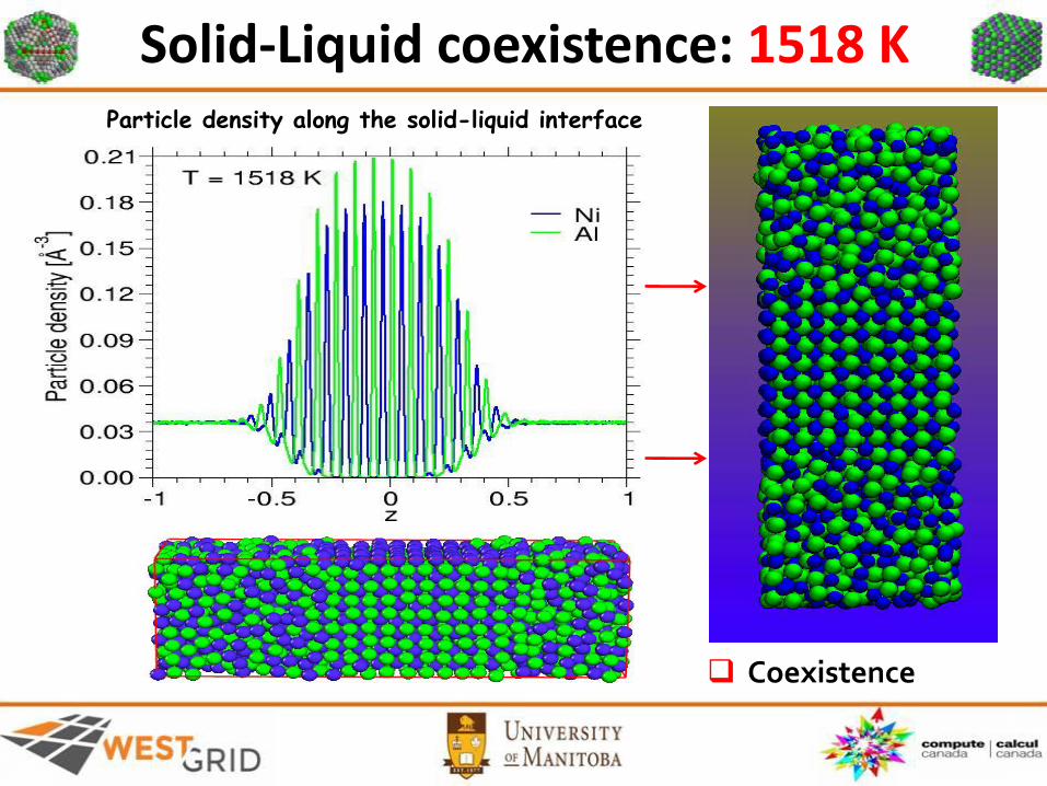
Solid-Liquid coexistence: 1518 K
Coexistence
Particle density along the solid-liquid interface

Crystallization of AlNi: 1460 K
CrystallizationParticle density along the solid-liquid interface

Crystal Growth: Diffusion Limitted
Why the solid-liquid interface velocity presents a maximum?
Maximum of 0.15 m/s at 180 KInterface velocity divided by the average self diffusion constant.Maximum due to decreasing of diffusion constant. Linear regime only up to 30 K of under-cooling.
What about the mass transport across the solid-liquid interface?
Solid-liquid interface velocity as a function of temperatureInset: as a function of under-cooling

Mass Transport across the interface
Order parameter to distinguish solid and liquid particles locally
compute the particle density and mass density profiles
Order parameter profile
Number of solid-like particles
Solid-liquid interface velocities from the number of solid-like particles
Diffusion along the interface
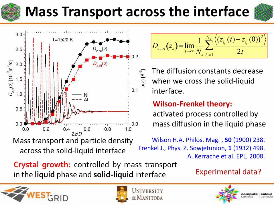
Mass Transport across the interface
Dzs , zs limt
1
Ns
(zis (t) zis (0))2
2tis 1
Ns
Mass transport and particle density across the solid-liquid interface
Wilson-Frenkel theory:activated process controlled by mass diffusion in the liquid phase
The diffusion constants decrease when we cross the solid-liquid interface.
Wilson H.A. Philos. Mag. , 50 (1900) 238.Frenkel J., Phys. Z. Sowjetunion, 1 (1932) 498.
A. Kerrache et al. EPL, 2008.
Crystal growth: controlled by mass transportin the liquid phase and solid-liquid interface Experimental data?

Comparison to Experimental Data terrestrial data (Assadi et al.) µg data (parabolic flight) , H. Hartmann (PhD thesis)
good agreement with experimental data
H. Assadi, et al., Acta Mat. 54, 2793 (2006).
A. Kerrache et al., EPL 81 (2008) 58001.

Glasses
Binary Metallic alloys:
Melting and crystallization. Solid-Liquid interfaces.Crystal growth from melt.Crystal growth is diffusion limited process.
Glasses:
How to prepare a glass using MD simulation? Glass Indentation using MD.

How to prepare a glass?
Glass preparation diagram
Glass preparation procedure:
Random configuration (N atoms). Liquid equilibration du at 5000 K (NVT). Cooling per steps of 100 K– (NVT). Glass equilibration at 300 K (NPT). Trajectory simulation at 300 K (NVE).
Model: MD Simulations (DL-POLY). Systems of N particules. Time step: 1 fs
SBN glasses: SiO2-B2O3-Na2O
R = [Na2O] / [B2O3] K = [SiO2] / [B2O3]
Cooling rates: 1012 to 1013 K/s

Glass Indentation
IndenterFree atoms
Fixed layer
N = 2.1 x 10⁶ atoms Temperature : 300 K Speed : 10 m/s Depth: ~3.0 nm
Movie provided by: Dimitrios KilymisUMR 5221 CNRS-Univ. Montpellier, France.

Acknowledgments
Prof. Dr. Jürgen Horbach, Dusseldorf, Germany.Prof. Dr. Kurt Binder, Mainz, Germany.Prof. A. Meyer and Prof. D. Herlach (DLR), Koln.
Prof. Normand Mousseau, Qc, Canada.Prof. Laurent J. Lewis, Qc, Canada.
Dr. Dimitrios Kilymis, Montpellier, France.Prof. Jean-Marc Delaye, CEA, France.
Dr. Victor Teboul, Angers, France.Prof. Hamid Bouzar, UMMTO, Tizi-Ouzou, Algeria.

Introduction to MD simulations
Setting and Running MD simulations (LAMMPS)
LAMMPS: Molecular Dynamics Simulator (introduction).
Building LAMMPS step by step.
Running LAMMPS (Input, Output, …).
Benchmark and performance tests.

Intorducion to LAMMPS
Large-scale Atomic / Molecular Massively Parallel Simulator

Start with LAMMPS
Large-scale Atomic / Molecular Massively Parallel Simulator
S. Plimpton, A. Thompson, R. Shan, S. Moore, A. Kohlmeyer … Sandia National Labs: http://www.sandia.gov/index.html
Home Page: http://lammps.sandia.gov/
Results: Papers: http://lammps.sandia.gov/papers.html Pictures: http://lammps.sandia.gov/pictures.htmlMovies: http://lammps.sandia.gov/movies.html
Resources:Online Manual: http://lammps.sandia.gov/doc/Manual.html Search the mailing list: http://lammps.sandia.gov/mail.html Subscribe to the Mailing List: https://sourceforge.net/p/lammps/mailman/lammps-users/
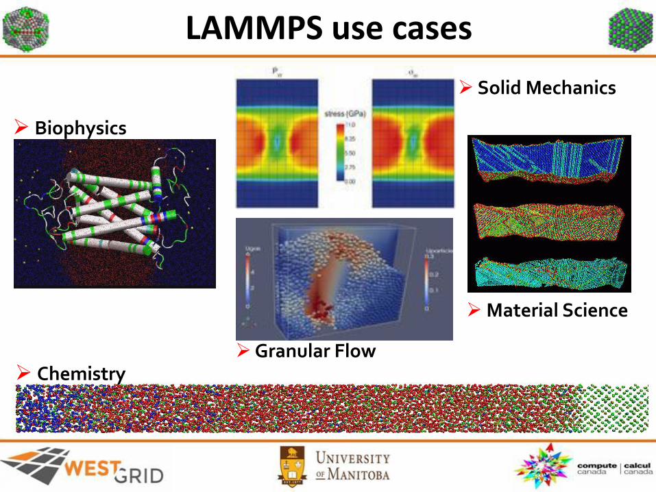
LAMMPS use cases
Biophysics
Chemistry
Solid Mechanics
Granular Flow
Material Science

LAMMPS Home Page
Big Picture CodeDocumentat
ionResults
RelatedTools
ContextUser
Support
Features Download Manual PublicationsPre/Post
processingAuthors Mail list
Non-features SourceForgeDeveloper
guidePictures
Pizza.py Toolkit
HistoryWorkshop
s
FAQLatest
features & bug fixes
Tutorials Movies
OffsiteLAMMPS
packages & tools
FundingUser
scripts and HowTos
Wish listUnfixed
bugs
MD to LAMMPS glossary
Benchmarks Visualization Open sourceContribute
to LAMMPS

Design of LAMMPS code
License LAMMPS is provided through GNU Public License
https://www.gnu.org/licenses/licenses.en.html#GPL Free to Use, Modify, and Distribute.Contribute to LAMMPS:
http://lammps.sandia.gov/contribute.html
Code Layout C++ and Object-Oriented approach Parallelization via MPI and OpenMP; runs on GPU. is invoked by commands through input scripts. possibility to customized output. could be interfaced with other codes (python, …).

How to obtain LAMMPS?
Download Page:http://lammps.sandia.gov/download.html
Distributions:Download a tarballGit checkout and updateSVN checkout and updatePre-built Ubuntu executablesPre-built binary RPMs for Fedora/RedHat/CentOS/openSUSEPre-built Gentoo executableOS X with HomebrewWindows installer packageApplying patches
Source Code
Executable Ubuntu
RPMs - Linux
Installation under Windows
Mac

Building LAMMPS Build from RPMsPre-built Ubuntu executablesPre-built binary RPMs for Fedora/RedHat/CentOS/openSUSEPre-built Gentoo executableOS X with Homebrew
Install under windowsWindows installer package
Build from source codeDownload a tarballGit checkout and updateSVN checkout and updateApplying patches
does not include all packages
for a customized installation, build from source files:
modules

LAMMPS under Windows Download Page: http://rpm.lammps.org/windows.html Installer: lammps-64bit-latest.exe
Directory:
Program Files\LAMMPS 64-bit 20171023
Executable under bin:
abf_integrate.exe ffmpeg.exe lmp_mpi.exe
restart2data.exe binary2txt.exe lmp_serial.exe
chain.exe msi2lmp.exe createatoms.exe
Execute: lmp_serial.exe < in.lammps

Building LAMMPS from source
http://lammps.sandia.gov/download.html#tar
Archive: lammps-stable.tar.gz

LAMMPS source overview
Download the source code: lammps-stable.tar.gz
LAMMPS directory: lammps-11Aug17
bench: Benchmark tests (potential, input and output files).
doc: documentation (PDF and HTML)
examples: input and output files for some simulations
lib: libraries to build before building LAMMPS
LICENSE and README files.
potentials: some of the force fields supported by LAMMPS
python: to invoke LAMMPS library from Python
src: source files (*.cpp, PACKAGES, USER-PACKAGES, …)
tools: some tools like xmovie (similar to VMD but only 2D).

Building LAMMPS
First: Build libraries if required.Choose a Makefile compatible with your systemChoose and install the packages you need.make package # list available packagesmake package-status (ps) # status of all packagesmake yes-package # install a single package in srcmake no-package # remove a single package from srcmake yes-all # install all packages in srcmake no-all # remove all packages from srcmake yes-standard (yes-std) # install all standard packages make no-standard (no-std) # remove all standard packagesmake yes-user # install all user packagesmake no-user # remove all user packages
Build LAMMPS:make machine # build LAMMPS for machine

Use GNU Make to build LAMMPS
machine is one of these from src/MAKE: # mpi = MPI with its default compiler # serial = GNU g++ compiler, no MPI
... or one of these from src/MAKE/OPTIONS: # icc_openmpi = OpenMPI with compiler set to Intel icc # icc_openmpi_link = Intel icc compiler, link to OpenMPI # icc_serial = Intel icc compiler, no MPI
... or one of these from src/MAKE/MACHINES: # cygwin = Windows Cygwin, mpicxx, MPICH, FFTW # mac = Apple PowerBook G4 laptop, c++, no MPI, FFTW 2.1.5 # mac_mpi = Apple laptop, MacPorts Open MPI 1.4.3, … # ubuntu = Ubuntu Linux box, g++, openmpi, FFTW3
... or one of these from src/MAKE/MINE: (write your own Makefile)

Building LAMMPS: demonstration
Download the latest stable version from LAMMPS home page. Untar the archive: tar -xvf lammps-stable.tar.gz Change the directory and list the files: cd lammps-11Aug17
bench bin doc examples lib LICENSE potentials python README src tools
Choose a Makefile (for example: machine=icc_openmpi)src/MAKE/OPTIONS/Makefile.icc_openmpi
Load the required modules (Intel, OpenMPI, …) Check the packages:
package, package-status, yes-package, no-package, … to build LAMMPS, run: make icc_openmpi Add or remove a package (if necessary), then recompile If necessary, edit Makefile and fix the path to libraries.

Running LAMMPS
Executable: lmp_machine
Files: Input File: in.lmp_file Potential: see examples and last slides for more details Initial configuration: can be generated by LAMMPS, or another program or home made program.
Interactive Execution: $ ./lmp_machine < in.lmp_file$ ./lmp_machine –in in.lmp_file
Redirect output to a file:$ ./lmp_machine < in.lmp_file > output_file$ ./lmp_machine –in in.lmp_file –l output_file

Command line options
Command-line options:
At run time, LAMMPS recognizes several optional command-line switches which may be used in any order.
-e or -echo, -h or –help, -i or –in, -k or –kokkos, -l or –log,
-nc or –nocite, -pk or –package, -p or –partition, -pl or –plog,
-ps or –pscreen, -r or –restart, -ro or –reorder, -sc or –screen,
-sf or –suffix, -v or –var
For example:mpirun -np 8 lmp_machine -l my.log -sc none -in in.alloympirun -np 8 lmp_machine < in.alloy > my.log

Overview of a simulation run
INPUT
• Initial positions
• Initial velocities
• Time step
• Mass
• PBC
• Units
• Potential
• Ensemble
• …. etc.
RUNNING
• Molecular Dynamics Simulation
(NPT, NVT, NVE)
• Minimization
• Monte Carlo
• Atomic to Continuum
OUTPUT
• Trajectories
• Velocities
• Forces
• Energy
• Temperature
• Pressure
• Density
• Snapshots
• Movies
• … etc.

Overview of a Simulation Run
Command Line: Every simulation is executed by supplying an input text script to the LAMMPS executable: lmp < lammps.in > log_lammps.txt
Parts of an input script: Initialize: units, dimensions, PBC, etc.Atomic positions (built in or read from a file) and velocities. Settings: Inter-atomic potential (pair_style, pair_coeff) Run time simulation parameters (e.g. time step) Fixes: operations during dynamics (e.g. thermostat)Computes: calculation of properties during dynamics
Run the simulation for N steps.

LAMMPS input example: LJ melt
Comment
Define units
Create the simulation box
Or read data from a file
Initialize the
velocities
Define the
potential

LAMMPS input example: LJ melt
Monitor the
neighbour list
Thermodynamic
Ensemble
Store the
trajectory
Log file:
customize output
Run the simulation
for N steps

LAMMPS: input commands
Initialization
Parameters: set parameters that need to be defined before atoms are created: units, dimension, newton, processors, boundary, atom_style, atom_modify.
If force-field parameters appear in the files that will be read:pair_style, bond_style, angle_style, dihedral_style, improper_style.
Atom definition: there are 3 ways to define atoms in LAMMPS. Read them in from a data or restart file via the read_data or read_restart commands. Or create atoms on a lattice (with no molecular topology), using these commands: lattice, region, create_box, create_atoms. Duplicate the box to make a larger one the replicate command.

LAMMPS: settings
Once atoms are defined, a variety of settings need to be specified: force field coefficients, simulation parameters, output options …
Force field coefficients: pair_coeff, bond_coeff, angle_coeff, dihedral_coeff, improper_coeff, kspace_style, dielectric, special_bonds.
Various simulation parameters:neighbor, neigh_modify, group, timestep, reset_timestep, run_style, min_style, min_modify.
Fixes: nvt, npt, nve, …
Computations during a simulation: compute, compute_modify, and variable commands.
Output options: thermo, dump, and restart commands.

Cutumize the output
thermo freq_stepsthermo_style style args
style = one or multi or custom args = list of arguments for a particular style
one args = none multi args = none customargs = list of keywords possible
keywords = step, elapsed, elaplong, dt, time, cpu, tpcpu, spcpu, cpuremain, part, timeremain, atoms, temp, press, pe, ke, etotal, enthalpy, evdwl, ecoul, epair, ebond, eangle, edihed, eimp, emol, elong, etail, vol, density, lx, ly, lz, xlo, xhi, ylo, yhi, zlo, zhi, xy, xz, yz, xlat, ylat, zlat, bonds, angles, dihedrals, impropers, pxx, pyy, pzz, pxy, pxz, pyz …..etc

Running LAMMPS: demonstration
After compiling LAMMPS, run some examples:
Where to start to learn LAMMPS?
Make a copy of the directory examples in your working directory.
Choose and example to run.
Indicate the right path to the executable.
Edit the input file and check all the parameters.
Check the documentation for the commands and their arguments.
Run the test case: lmp_icc_openmpi < in.melt .
Check the output files (log files), plot the thermodynamic
properties, ...

LAMMPS: output example
LAMMPS (30 Jul 2016) using 1 2 OpenMP thread(s) per MPI task# 3d Lennard-Jones melt
units ljatom_style atomiclattice fcc 0.8442Lattice spacing in x,y,z = 1.6796 1.6796 1.6796region box block 0 10 0 10 0 10create_box 1 box
Created orthogonal box = (0 0 0) to (16.796 16.796 16.796) 2 by 2 by 3 MPI processor grid
create_atoms 1 boxCreated 4000 atoms
mass 1 1.0

LAMMPS: output examplethermo 100run 25000Neighbor list info ...
1 neighbor list requests update every 20 steps, delay 0 steps, check no max neighbors/atom: 2000, page size: 100000 master list distance cutoff = 2.8 ghost atom cutoff = 2.8 binsize = 1.4 -> bins = 12 12 12Memory usage per processor = 2.05293 Mbytes
Step Temp E_pair E_mol TotEng Press 0 3 -6.7733681 0 -2.2744931 -3.7033504 100 1.6510577 -4.7567887 0 -2.2808214 5.8208747 200 1.6393075 -4.7404901 0 -2.2821436 5.9139187 300 1.6626896 -4.7751761 0 -2.2817652 5.756386

LAMMPS: output example25000 1.552843 -4.7611011 0 -2.432419 5.7187477
Loop time of 15.4965 on 12 procs for 25000 steps with 4000 atomsPerformance: 696931.853 tau/day, 1613.268 timesteps/s90.2% CPU use with 12 MPI tasks x 1 OpenMP threads
MPI task timing breakdown:Section | min time | avg time | max time |%varavg| %total-----------------------------------------------------------------------------Pair | 6.6964 | 7.1974 | 7.9599 | 14.8 | 46.45Neigh | 0.94857 | 1.0047 | 1.0788 | 4.3 | 6.48Comm | 6.0595 | 6.8957 | 7.4611 | 17.1 | 44.50Output | 0.01517 | 0.01589 | 0.019863 | 1.0 | 0.10Modify | 0.14023 | 0.14968 | 0.16127 | 1.7 | 0.97Other | | 0.2332 | | | 1.50
Total wall time: 0:00:15

Potential Benchmark
1. granular2. fene3. lj4. dpd5. eam6. sw7. rebo8. tersoff9. eim10. adp11. meam12. peri
13. spce14. protein15. gb16. reax_AB17. airebo18. reaxc_rdx19. smtbq_Al20. vashishta_table_sio221. eff22. comb23. vashishta_sio224. smtbq_Al2O3
Parameters:
24 different cases. Number of particles: about 32000 CPUs = 1MD steps = 1000 Record the simulation time and the time used in computing the interactions between particles.

Potential Benchmark

Performance Test: Tersoff potential
CPU time used for computing the interactions between particles as a function the number of processors for different system size.

Performance Test: Tersoff potential
CPU time used for computing the interactions between particles as a function the number of processors for different system size.

Performance Test: Tersoff potential
Size, shape of the system. Number of processors. size of the small units. correlation between the communications and the number of small units. Reduce the number of cells to reduce communications.
Domain decomposition

Learn more about LAMMPS
Resources:Online Manual: http://lammps.sandia.gov/doc/Manual.html Search the mailing list: http://lammps.sandia.gov/mail.htmlMailing List:https://sourceforge.net/p/lammps/mailman/lammps-users/
Home Page: http://lammps.sandia.gov/
Examples: deposit, friction, micelle, obstacle, qeq, streitz, MC, body, dipole, hugoniostat, min, peptide, reax, tad, DIFFUSE, colloid, indent, msst, peri, rigid , vashishta, ELASTIC, USER, comb, eim, nb3b, pour, shear, voronoi, ELASTIC_T, VISCOSITY, coreshell, ellipse, meam, neb, prd, snap, HEAT, accelerate, crack, flow, melt, nemd
Results: Papers: http://lammps.sandia.gov/papers.html Pictures: http://lammps.sandia.gov/pictures.htmlMovies: http://lammps.sandia.gov/movies.html

Introduction to MD Simulations
Thanks to LAMMPS developers
Thanks to LAMMPS contributors
Thank you for your attention
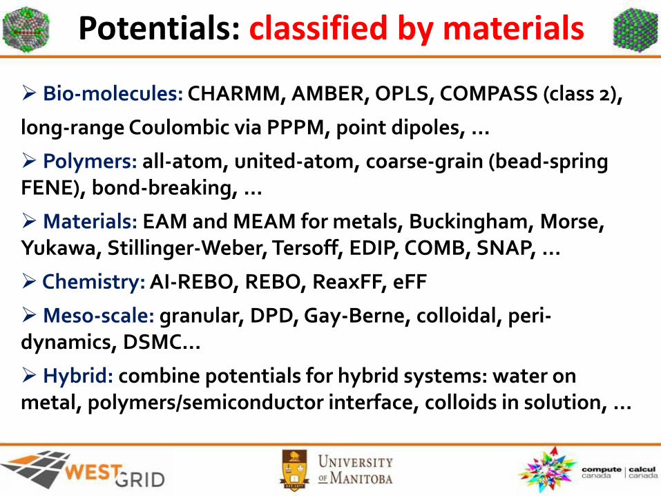
Potentials: classified by materials
Bio-molecules: CHARMM, AMBER, OPLS, COMPASS (class 2),
long-range Coulombic via PPPM, point dipoles, ...
Polymers: all-atom, united-atom, coarse-grain (bead-spring FENE), bond-breaking, …
Materials: EAM and MEAM for metals, Buckingham, Morse, Yukawa, Stillinger-Weber, Tersoff, EDIP, COMB, SNAP, ...
Chemistry: AI-REBO, REBO, ReaxFF, eFF
Meso-scale: granular, DPD, Gay-Berne, colloidal, peri-dynamics, DSMC...
Hybrid: combine potentials for hybrid systems: water on metal, polymers/semiconductor interface, colloids in solution, …

Potentials: classified by functional form
Pair-wise potentials: Lennard-Jones, Buckingham, ...
Charged Pair-wise Potentials: Coulombic, point-dipole
Many-body Potentials: EAM, Finnis/Sinclair, modified EAM (MEAM), embedded ion (EIM), Stillinger-Weber, Tersoff, AI-REBO, ReaxFF, COMB
Coarse-Grained Potentials: DPD, GayBerne, ...
Meso-scopic Potentials: granular, peri-dynamics
Long-Range Electrostatics: Ewald, PPPM, MSM
Implicit Solvent Potentials: hydrodynamic lubrication, Debye
Force-Field Compatibility with common: CHARMM, AMBER, OPLS, GROMACS options


