119
WEYL-INVARIANT HIGHER CURVATURE GRAVITY THEORIES
A THESIS SUBMITTED TOTHE GRADUATE SCHOOL OF NATURAL AND APPLIED SCIENCES
OFMIDDLE EAST TECHNICAL UNIVERSITY
BY
SUAT DENGIZ
IN PARTIAL FULFILLMENT OF THE REQUIREMENTSFOR
THE DEGREE OF DOCTOR OF PHILOSOPHYIN
PHYSICS
SEPTEMBER, 2014

Approval of the thesis:
WEYL-INVARIANT HIGHER CURVATURE GRAVITY THEORIES
submitted by SUAT DENGIZ in partial fulllment of the requirements for thedegree of Doctor of Philosophy in Physics Department, Middle East
Technical University by,
Prof. Dr. Canan ÖzgenDean, Graduate School of Natural and Applied Sciences
Prof. Dr. Mehmet ZeyrekHead of Department, Physics
Prof. Dr. Bayram TekinSupervisor, Physics Dept., METU
Examining Committee Members:
Prof. Dr. Atalay KarasuPhysics Dept., METU
Prof. Dr. Bayram TekinPhysics Dept., METU
Prof. Dr. Yldray OzanMathematics Dept., METU
Prof. Dr. Altu§ ÖzpineciPhysics Dept., METU
Assoc. Prof. Dr. Fatma Muazzez im³irMathematics Dept., Hittite University
Date:
I hereby declare that all information in this document has been ob-
tained and presented in accordance with academic rules and ethical
conduct. I also declare that, as required by these rules and conduct,
I have fully cited and referenced all material and results that are not
original to this work.
Name, Last Name: SUAT DENGIZ
Signature :
iv
ABSTRACT
WEYL-INVARIANT HIGHER CURVATURE GRAVITY THEORIES
Dengiz, Suat
Ph.D., Department of Physics
Supervisor : Prof. Dr. Bayram Tekin
SEPTEMBER, 2014, 103 pages
In this thesis, Weyl-invariant extensions of three-dimensional New Massive Grav-
ity, generic n-dimensional Higher Curvature Gravity theories and three-dimensional
Born-Infeld gravity theory are analyzed in details. As required byWeyl-invariance,
the actions of these gauge theories do not contain any dimensionful parameter,
hence the local symmetry is spontaneously broken in (Anti) de Sitter vacua in
analogy with the Standard Model Higgs mechanism. In at vacuum, symmetry
breaking mechanism is more complicated: The dimensionful parameters come
from dimensional transmutation in the quantum eld theory; therefore, the con-
formal symmetry is radiatively broken (at two loop level in 3-dimensions and
at one-loop level in 4-dimensions) à la Coleman-Weinberg mechanism. In the
broken phases, save for New Massive Gravity, the theories generically propagate
with a unitary (tachyon and ghost-free) massless tensor, massive (or massless)
vector and massless scalar particles for the particular intervals of the dimension-
less parameters. For New Massive Gravity, there is a massive Fierz-Pauli-type
graviton. Finally, it is shown that n-dimensional Weyl-invariant Einstein-Gauss-
v

Bonnet theory is the only unitary higher dimensional Weyl-invariant Quadratic
Curvature Gravity theory.
Keywords: Weyl-invariance, New Massive Gravity, Higher Curvature Gravity
Theories, Born-Infeld Gravity theory, Spontaneously Symmetry Breaking, Ra-
diatively Symmetry Breaking, (Anti) de Sitter spaces, Weyl-invariant Einstein-
Gauss-Bonnet theory
vi

ÖZ
YÜKSEK MERTEBEDEN ERL WEYL-DEMEZL KÜTLE-ÇEKMKURAMLARI
Dengiz, Suat
Doktora, Fizik Bölümü
Tez Yöneticisi : Prof. Dr. Bayram Tekin
2014 , 103 sayfa
Bu tez çal³masnda, Weyl-de§i³mez bir ³ekilde geni³letilmi³ üç boyutlu Yeni
Kütleli Kütle-çekim, genel n-boyutlu Yüksek Mertebeden E§rili Kütle-çekim
teorileri ve üç boyutlu Born-Infeld Kütle-çekim teorisi detayl ³ekilde analiz
edildi. Weyl-de§i³mez tarafndan gerekli görüldü§ü üzere, bu ayar teorilerinin
eylem integralleri birimli parametre içermezler, dolaysyla lokal simetri Stan-
dard Model Higgs Mekanizmasndaki gibi (Anti) de Sitter vakumlarnda kendil-
i§inden krlr. Düz uzay-zaman vakumunda, simetri krlma mekanizmas çok
karma³kdr: Birimli parametreler kuantum teorisindeki birimsel dönü³ümden
gelir; bundan dolay konformal simetri Coleman-Weinberg mekanizmasna ben-
zer olarak halka seviyesinde (3-boyutta iki-halka seviyesinde ve 4-boyutta bir-
halka seviyesinde) krlr. Simetrinin krld§ fazlarda, Yeni Kütleli Kütle-çekim
teorisi hariç, genel olarak teoriler boyutsuz parametrelerin özel aralklarnda
üniter (takyon ve hayalet olmakszn) bir kütlesiz tensör, bir kütleli (veya kütle-
vii

siz) vektör ve bir kütlesiz skaler parçacklar olarak hareket ederler. Yeni Kütleli
Kütle-çekim teorisinde ise Fierz-Pauli-tipi kütleli bir graviton vardr. Son olarak,
Weyl-de§i³mez Einstein-Gauss-Bonnet teorisinin n-boyutlu Weyl-de§i³mez ik-
inci dereceden Kütle-çekim teorileri içerisinde üniter olan tek teori oldu§u gös-
terildi.
Anahtar Kelimeler: Weyl-de§i³mez, Yeni Kütleli Kütle-çekim, Yüksek Mertebe-
den Kütle-çekim teorileri, Born-Infeld Kütle-çekim teorisi, Kendili§inden Simetri
Krlmas, Halka Mertesi Simetri Krlmas, (Anti) de Sitter uzaylar, Weyl-
de§i³mez Einstein-Gauss-Bonnet teori
viii

To My mother and father and also My nieces and nephews Zeynep Rüya, Dicle
Ezo, Samet and Muhammed
ix
ACKNOWLEDGEMENTS
Frankly speaking, it became very hard for me how to express my ideas about
my supervisor Professor Bayram Tekin. Throughout this period, what I have
certainly concluded is that Professor Bayram Tekin is actually the scientist who
I have always dreamt to be since I was a child. I would like to express my
deepest gratitude to him, who not only provided me to approach my aim but
also demonstrated which features a unique, totally universal scientist with an
enormous and innite dimensional hearth must have. He taught me, regardless
to the research eld and also how hard, how much important any scientic
information is, and also encouraged me how intensely and eagerly to work till
mornings in order to capture them. I would like to appreciate his guidance,
innite patience and support in all aspects which in fact supplied me to write
this thesis. It is a great honor and privilege for me to be his student. Finally, I
would also like to express all my best wishes to Professor Bayram Tekin's source
of energy sweet Elif Ada who reminds me my niece sweet heart Dicle Ezo who
I rarely see. Ada is the youngest and funniest informal member of our research
group, and also who always conjectured the constant ′′5′′ to be the universal
answer to any question.
I would also like to thank to my funny and admirably kind roommate, close friend
and collaborate Ercan Klçarslan for all his support throughout this period.
His scientic motivation, cleverness and unique approach to the problems have
always aected me.
In addition to this, I would like to express my deepest gratitude and thanks to
the following people particularly to Professor Roman Jackiw, a world-leading
theoretical physicist, for their critical advices and supports in all aspects up to
now: Professor Roman Jackiw, Professor Atalay Karasu, Professor Tekin Dereli,
Professor Altu§ Özpineci, Professor Ay³e Kalkanl Karasu, Assoc. Professor
x
M. Reza Tanhayi, Professor Metin Önder, Professor Müge Boz Evinay, Profes-
sor Yi§it Gündüç, Professor Yldray Ozan, Assoc. Professor Fatma Muazzez
im³ir, Professor Altan Baykal, Assoc. Professor Ahmet Mecit Özta³, Professor
Fatih Ya³ar, Professor Turan Özbey, Professor Mustafa Savc, Professor Bülent
Akno§lu, Assoc. Professor Hatice Kökten, Assoc. Professor Mehmet Dilaver,
Assist. Professor Tahsin Ç. i³man, Dr. Ibrahim Güllü, Dr. Cesim Dumlu,
Zeynep Acuner, M. Mirac Serim, Ender Eylenceo§lu, Ceren Sibel Sayn, Mecit
Demir, Ibrahim Burak Ilhan, Danjela Çerri, Ekrem Yavuz (recently died at the
age of 28), Deniz Özen, Kezban Ta³seten Ata, Emel Alta³, Özge Bayrakl, M.
Ali Olpak, Tuna Yldrm, Bar³ Çelik, Erdinç Da§deviren, Mahmut Kavu³an,
Begüm Barut, Gözde B. Çiçek, Deniz O. Devecio§lu, Gökhan Alkaç and Merve
Demirta³.
Finally, my special thanks are to the leading Otorhinolaryngologist Professor Dr.
Mehmet Hakan Korkmaz and my close friend Cardiologist Dr. Cengiz Burak for
their respectable supports in all aspects throughout this period. I would like
to especially thank Professor Dr. Mehmet Hakan Korkmaz for his admirable
scientic soul and kindness to a student who would like to do the universal
science within strict and tough conditions.
During my Ph.D. education, I have been supported by The Scientic and Tech-
nological Research Council of Turkey (TÜBTAK) with the scholarships in two
1001 projects with grant numbers 113F155 and 109T748.
xi

TABLE OF CONTENTS
ABSTRACT . . . . . . . . . . . . . . . . . . . . . . . . . . . . . . . . . v
ÖZ . . . . . . . . . . . . . . . . . . . . . . . . . . . . . . . . . . . . . . . vii
ACKNOWLEDGEMENTS . . . . . . . . . . . . . . . . . . . . . . . . . x
TABLE OF CONTENTS . . . . . . . . . . . . . . . . . . . . . . . . . . xii
LIST OF FIGURES . . . . . . . . . . . . . . . . . . . . . . . . . . . . . xv
CHAPTERS
I INTRODUCTION . . . . . . . . . . . . . . . . . . . . . . . . . 1
I.1 Higher Order Gravity Theories . . . . . . . . . . . . . . 6
I.1.0.1 New Massive Gravity: A Three Di-mensional Theory . . . . . . . . . . 9
I.2 Conformal Invariance . . . . . . . . . . . . . . . . . . . 10
I.3 Spontaneous Symmetry Breaking . . . . . . . . . . . . . 12
I.3.1 Higgs Mechanism . . . . . . . . . . . . . . . . 14
I.3.2 Coleman-Weinberg Mechanism in n = 4 andn = 3 Dimensions . . . . . . . . . . . . . . . . 18
II HIGGS MECHANISM FOR NEW MASSIVE GRAVITY ANDWEYL-INVARIANT EXTENSIONS OF HIGHER-DERIVATIVETHEORIES . . . . . . . . . . . . . . . . . . . . . . . . . . . . . 33
II.1 Weyl Transformation . . . . . . . . . . . . . . . . . . . . 34
xii
II.2 Weyl-Invariant n-Dimensional Quadratic Curvature Grav-ity Theories . . . . . . . . . . . . . . . . . . . . . . . . . 38
II.2.1 Weyl-invariant NewMassive Gravity and relatedSymmetry Breaking Mechanism . . . . . . . . 39
II.2.2 Weyl-Invariant Born-Infeld theories . . . . . . 44
III UNITARITY OF WEYL-INVARIANT NEW MASSIVE GRAV-ITY AND GENERATION OF GRAVITON MASS VIA SYM-METRY BREAKING . . . . . . . . . . . . . . . . . . . . . . . . 47
III.1 Perturbative Expansion of the Action up to Quadratic-Order . . . . . . . . . . . . . . . . . . . . . . . . . . . . 48
III.1.1 Scale-Invariant Gauge-Fixing Condition . . . . 52
III.1.2 Redenition of the Metric Fluctuation . . . . . 53
IV WEYL-INVARIANT HIGHER CURVATURE GRAVITY THE-ORIES IN N DIMENSIONS . . . . . . . . . . . . . . . . . . . . 57
IV.1 Perturbative Expansion about (A)dS Vacua . . . . . . . 58
IV.1.1 Scale-Invariant Gauge-Fixing Condition . . . . 62
IV.1.2 Redenition of the Metric Fluctuation . . . . . 62
IV.2 Fundamental Excitations of the Theory . . . . . . . . . 64
V CONCLUSION . . . . . . . . . . . . . . . . . . . . . . . . . . . 71
REFERENCES . . . . . . . . . . . . . . . . . . . . . . . . . . . . . . . . 73
VI FIELD EQUATION FOR THE PARTICLES . . . . . . . . . . 79
VI.1 Field Equation for gµν . . . . . . . . . . . . . . . . . . . 80
VI.2 Field Equation for Aµ . . . . . . . . . . . . . . . . . . . 86
xiii
VII PERTURBATIVE EXPANSION OF THEGENERICN -DIMENSIONALWEYL-INVARIANT HIGHER CURVATURE GRAVITY THE-ORIES . . . . . . . . . . . . . . . . . . . . . . . . . . . . . . . 87
VII.1 Second Order Expansions of the Curvature Terms . . . . 88
VII.2 Second Order Expansion of the Action . . . . . . . . . . 90
CURRICULUM VITAE . . . . . . . . . . . . . . . . . . . . . . . . . . . 101
xiv

LIST OF FIGURES
FIGURES
Figure I.1 Tree-level scattering amplitude via one graviton exchange be-
tween two point-like locally conserved sources. . . . . . . . . . . . . 8
Figure I.2 Mexican-hat-like Higgs Potential. . . . . . . . . . . . . . . . 13
Figure I.3 One-loop corrections resulted from the sum of innitely num-
bers of quartically self-interacting scalar elds. . . . . . . . . . . . . 22
Figure I.4 Symmetry breaking via Coleman-Weinberg mechanism. The
blue and red lines stand for tree-level and three-level plus one-loop
eective potentials, respectively: Observe that after adding the one-
loop corrections to the tree-level potential, the minimum is converted
and the new minimum occurs at a nonzero point <Φ>M
. . . . . . . . . 24
Figure I.5 Two scalar loops. . . . . . . . . . . . . . . . . . . . . . . . . 29
Figure I.6 One scalar and one gauge loop. . . . . . . . . . . . . . . . . . 29
Figure I.7 θ-shape diagram. . . . . . . . . . . . . . . . . . . . . . . . . 30
Figure I.8 θ-shape diagram with two scalar and one gauge propagators. 31
Figure I.9 θ-shape diagram with two gauge and one scalar propagators. 32
xv

xvi
CHAPTER I
INTRODUCTION
Quantum Mechanics and Einstein's Special and General theories of relativity
(SR and GR, respectively) are probably the greatest achievements of physics in
the 20th-century. Roughly speaking, Quantum Theory is the theory of small-
scales whereas the SR is of high-velocity and GR is of the large-scales. As it
is known, each of these theories has in fact shortcomings: Quantum Mechanics
is not a relativistic one. On the other side, GR fails to be a Quantum The-
ory. Therefore, reconciling Quantum Mechanics with SR yields a well-behaved
relativistic version of Quantum Mechanics called Quantum Field Theories. In
the framework of Quantum Field Theories, the coupling constants generically
involve the information of basic interactions of given quantum elds. Depending
on values of the coupling constants (which are actually not constants at all!),
there are two distinct and fundamental approaches in this new context, namely
perturbative and non-perturbative methods. In the non-perturbative method,
the related coupling constants of the elds are so large that they prevent one
to approach the theory perturbatively. On the other side, when the coupling
constants are satisfactorily small, one can then approach the theories perturba-
tively (namely in a power series expansion in terms of the coupling constants) in
order to determine the fundamental behaviors of the elds: Here, by using the
noninteracting elds, one can evaluate the explicit contributions coming from
any desired order by expanding the coupling constants in the power-series up to
a proper order. Symbolically, the corresponding interactions are always denoted
by the connected Feynman diagrams in which it is assumed that these interac-
tions are carried via the exchange of virtual particles. Moreover, in Quantum
1

Field Theories, these virtual mediators or (interacting) quantum elds can also
move in the loops whose momenta are allowed to be any value, that is to say,
they can acquire any frequency from zero to innity. And interestingly, these
higher-order eects generically do modify the physical quantities of the elds
such as masses, propagator structures, eective potentials etc. Therefore, in
order to nd the exact values of these physical quantities, one has to evalu-
ate contributions coming from the radiative corrections by summing over all
the allowed momentums (i.e., from zero to innity) that particles can receive
throughout the loops. But, these sums (or integrals) often diverge, as the mo-
mentum goes to zero (IR-divergence) or to innity (UV-divergence). In general,
these disturbing innities in the extreme limits can be resolved by choosing an
appropriate regularization scheme, to get rid o the divergences. For instance,
one can assume a cut-o scale Λ which will cut the integral at a nite value and
thus eliminate those disturbing innities. Generically, one needs cut-os both at
the IR and UV regions. But, in this case, the scattering amplitudes and also the
coupling constants will inevitably depend on the cut-o, and hence the theory
becomes an eective one, meaning the theory is valid below the, say UV, cut-o.
Alternatively, one can follow the dimensional regularization [1, 2] where integrals
are evaluated at complex n-dimensions, or Pauli-Villars method [3] in which the
bare propagators are replaced with the ones which involve very heavy ghosts to
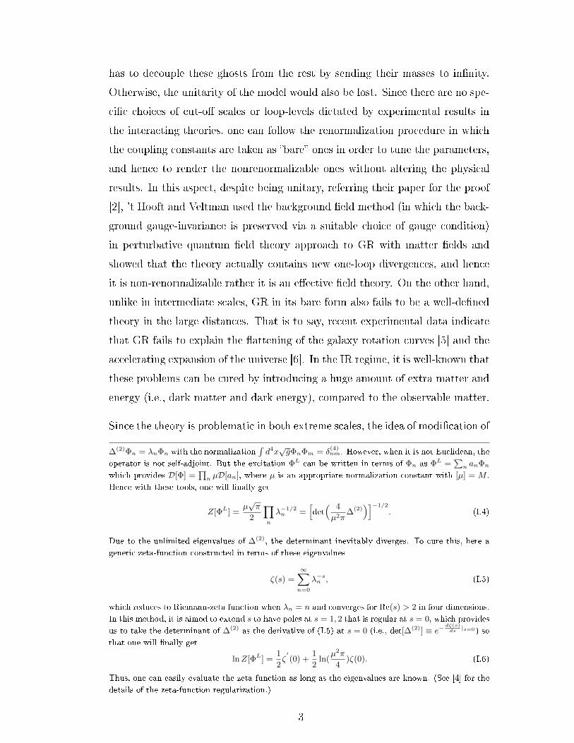
regularize the divergent integrals1. After the regularization is carried out, one1 There is also another regularization process dubbed zeta-function regularization which is
used in order to drop out divergences in determinant of the operator occurred during path integrals
of elds: That is, let us suppose that the vacuum to vacuum transition amplitude for a generic
gravity-coupled-scalar-eld theory in a curved spacetime
Z ≡∫D[g]D[Φ] eiS[g,Φ], (I.1)
is given. Here ~ is set to 1. Then, with the redenitions gµν = gµν + hµν and Φ = Φ0 + ΦL, (I.1)
turns into
lnZ ≡ iS[g,Φ0] + ln
∫D[h] eiS
(2)[h] + ln
∫D[ΦL] eiS
(2)[ΦL]. (I.2)
Furthermore, the quadratic part of ΦL in (I.2) can also be written as
S(2)[ΦL] = −1
2
∫d4x√−gΦL∆(2)ΦL, (I.3)
where ∆(2) is the related second-order operator composed of gµν and ΦL. (Note that the metric part
can also be converted in the similar form. But in that case one needs to also dene a Fadeev-Popov
ghost in order to x the gauge freedom that causes degeneracies in the operator.) It is known that if
the background metric is Euclidean, ∆(2) becomes real, elliptic and self-adjoint so that it has complete
spectrum of eigenvectors Φn with real eigenvalues λn. Therefore, after Wick rotation, one will get
2
has to decouple these ghosts from the rest by sending their masses to innity.
Otherwise, the unitarity of the model would also be lost. Since there are no spe-
cic choices of cut-o scales or loop-levels dictated by experimental results in
the interacting theories, one can follow the renormalization procedure in which
the coupling constants are taken as bare ones in order to tune the parameters,
and hence to render the nonrenormalizable ones without altering the physical
results. In this aspect, despite being unitary, referring their paper for the proof
[2], 't Hooft and Veltman used the background eld method (in which the back-
ground gauge-invariance is preserved via a suitable choice of gauge condition)
in perturbative quantum eld theory approach to GR with matter elds and
showed that the theory actually contains new one-loop divergences, and hence
it is non-renormalizable rather it is an eective eld theory. On the other hand,
unlike in intermediate scales, GR in its bare form also fails to be a well-dened
theory in the large distances. That is to say, recent experimental data indicate
that GR fails to explain the attening of the galaxy rotation curves [5] and the
accelerating expansion of the universe [6]. In the IR regime, it is well-known that
these problems can be cured by introducing a huge amount of extra matter and
energy (i.e., dark matter and dark energy), compared to the observable matter.
Since the theory is problematic in both extreme scales, the idea of modication of
∆(2)Φn = λnΦn with the normalization∫d4x√gΦnΦm = δ
(4)nm. However, when it is not Euclidean, the
operator is not self-adjoint. But the excitation ΦL can be written in terms of Φn as ΦL =∑n anΦn
which provides D[Φ] =∏n µD[an], where µ is an appropriate normalization constant with [µ] = M .
Hence with these tools, one will nally get
Z[ΦL] =µ√π
2
∏n
λ−1/2n =
[det( 4
µ2π∆(2)
)]−1/2
. (I.4)
Due to the unlimited eigenvalues of ∆(2), the determinant inevitably diverges. To cure this, here a
generic zeta-function constructed in terms of these eigenvalues
ζ(s) =
∞∑n=0
λ−sn , (I.5)
which reduces to Riemann-zeta function when λn = n and converges for Re(s) > 2 in four dimensions.
In this method, it is aimed to extend s to have poles at s = 1, 2 that is regular at s = 0, which provides
us to take the determinant of ∆(2) as the derivative of (I.5) at s = 0 (i.e., det[∆(2)] ≡ e−dζ(s)ds|s=0) so
that one will nally get
lnZ[ΦL] =1
2ζ′(0) +
1
2ln(
µ2π
4)ζ(0). (I.6)
Thus, one can easily evaluate the zeta-function as long as the eigenvalues are known. (See [4] for the
details of the zeta-function regularization.)
3

GR (or even replacing it with a new one) has received valuable attention. For this
reason, various approaches have been proposed in order to construct a consistent
and predictive UV and IR-complete gravity theory. Perhaps, one can collect all
these approaches in two families: Firstly, one can totally change the background
spacetime to a new (higher or lower dimensional one at high energies) one.
Probably, in this family, the most known example is String theory which was
developed in higher-dimensional manifolds. Despite its undesired features such
as its great number of vacua, it achieves not only to quantize gravity but also
provides a unied theory. Secondly, one might not alter the 4−dimensional
arena and use the experience obtained from Quantum Field Theories in order
to obtain the desired tree (and/or loops)-level propagator structure, and hence
(self-)interactions. In this point of view, for instance, one can assume higher
order curvature corrections to pure GR [7] such that they will be suppressed in
the lower frequency regimes, but they turn to be important as one goes to higher
frequency regimes. [In fact, at low energies String theory also yield such higher
order gravity theories.] Alternatively, one can assume a proper extra symmetry
that might spoil out the above mentioned one-loop divergence of GR. Here due
to the several reasons, the conformal symmetry is a candidate for this aim. For
instance, since according to the SR context, the masses of the excitations lose
their importance as the energy scale is increased. Therefore, it is expected that
such a well-behaved gravity theory will not contain any dimensionful parameter
in the extremely high energy regions, say Planck-scale or beyond. However, GR
has a dimensionful parameter with a mass dimension −2, that is the Newton's
constant. So somehow Newton's constant must be upgraded to a eld. Since
conformal symmetry does not accept any dimensionful parameter, so, it might
resolve the above mentioned problem of GR in extremely high energy scales.
Hence, being free of dimensionful parameters can provide a renormalized gravity
theory at least in the power-counting point of view.
In this thesis, we analyze the Weyl-invariant modications of various Higher
Order Gravity theories and also study the stability and unitarity of them as
well as the corresponding symmetry-breaking mechanisms at low energies for
the generation of the masses for fundamental excitations propagated about con-
4
stant curvature vacua, as well as the appearance of the Newton's constant. Our
discussion will be based on the following papers:
1. S. Dengiz, and B. Tekin, Higgs mechanism for New Massive Gravity and
Weyl-invariant extensions of Higher-Derivative Theories, Phys. Rev. D
84, 024033 (2011) [8].
2. M. Reza Tanhayi, S. Dengiz, and B. Tekin, Unitarity of Weyl-Invariant
New Massive Gravity and Generation of Graviton Mass via Symmetry
Breaking, Phys. Rev. D 85, 064008 (2012) [9].
3. M. Reza Tanhayi, S. Dengiz, and B. Tekin, Weyl-Invariant Higher Curva-
ture Gravity Theories in n Dimensions, Phys. Rev. D 85, 064016 (2012)
[10].
In the rst paper, Weyl-invariant extension of New Massive Gravity, generic
n-dimensional Quadratic Curvature Gravity theories and 3-dimensional Born-
Infeld gravity are presented. As required by the Weyl-invariance, Lagrangian
densities of these Weyl-invariant Higher Curvature Gravity theories are free of
any dimensionful parameter. In addition to the constructions of those gauge
theories, the symmetry breaking mechanisms in the Weyl-invariant New Massive
Gravity is also studied in some detail. Here the structure of the symmetry
breaking directly depends on the type of background wherein one works: the
Weyl symmetry is spontaneously broken by the (Anti) de Sitter vacua. On
the other side, radiative corrections at two-loop level break the symmetry in
at backgrounds and thus these broken phases of the model provide mass to
graviton.
In the second paper, the particle spectrum and hence the stability of the Weyl-
invariant New Massive Gravity around its maximally-symmetric vacua are stud-
ied in detail. Since the model contains various non-minimally coupled terms,
the stability and unitarity of the model are determined by expanding the action
up to the second-order in the uctuations of the elds. Here it is demonstrated
that the model fails to be unitary in de Sitter space. Moreover, it is shown that
the Weyl-invariant New Massive Gravity generically propagates with a unitary
5

massive graviton, massive (or massless) vector particle and massless scalar par-
ticle in the particular domains of parameters around its Anti-de Sitter and at
vacua. Thus, as indicated in the rst paper, the masses of the fundamental
excitations of the model are generated as a result of breaking of the conformal
symmetry.
Finally, in the last paper, stability and unitarity of the Weyl-invariant extension
of the n-dimensional Quadratic Curvature theories are analyzed. From the per-
turbative expansion of the action, it is shown that, save for the Weyl-invariant
New Massive Gravity, the graviton is massless. Moreover, it is shown that the
Weyl-invariant Gauss-Bonnet model can only be the Weyl-invariant Quadratic
Curvature Gravity theory in higher dimensions.
To be able to give a detailed exposition on the contents of these 3 papers, let us
briey review the required background material 2: The basics of the higher curva-
ture gravity theories, the conformal transformations and Spontaneous-Symmetry
Breaking via Standard Model Higgs Mechanism and Radiative-corrections in the
remainder of this chapter.
I.1 Higher Order Gravity Theories
Even though pure GR has a unitary massless spin-2 particle (the graviton), as
mentioned above, there occurs divergences at the higher-order corrections due to
the graviton self-interactions. To stabilize this nonrenormalization at least in the
power-counting aspects, one can add higher powers of curvature scalar terms to
the bare action in order to convert the propagator structure into the desired form
such that the higher order part will be suppressed in the large-scales so they can
be ignored, whereas they become important as the energy scale increases. Since
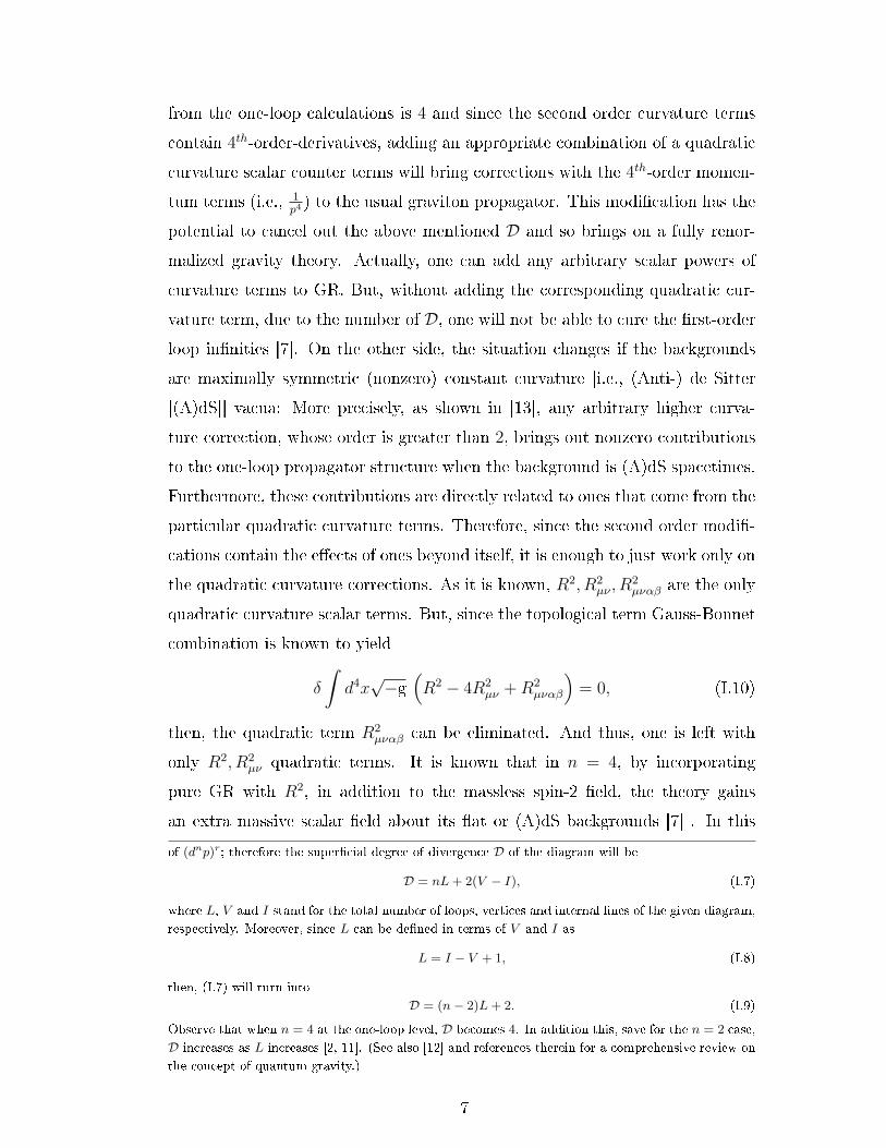
the supercial degree of divergence D of the four-dimensional GR 3 that arises
2 In this dissertation, we follow two conventions: In the pure Quantum Field Theory parts in
this chapter, we are following the mostly-negative signature. On the other hand, in all the gravity
parts throughout this thesis, we are following the mostly-plus signature and also Riemann and Ricci
tensors are Rµνρσ = ∂ρΓµσν + ΓµραΓασν − ρ↔ σ and Rνσ = Rµνµσ, respectively.
3 GR's action is built from the Ricci scalar R which involves second-order derivatives of the
metric. Hence, the momentum-space propagator of the graviton will behave as 1p2
whereas each
vertex propagates as p2. Since in generic n dimensions, the r-loop diagrams will contain integration
6
from the one-loop calculations is 4 and since the second order curvature terms
contain 4th-order-derivatives, adding an appropriate combination of a quadratic
curvature scalar counter terms will bring corrections with the 4th-order momen-
tum terms (i.e., 1p4 ) to the usual graviton propagator. This modication has the
potential to cancel out the above mentioned D and so brings on a fully renor-
malized gravity theory. Actually, one can add any arbitrary scalar powers of
curvature terms to GR. But, without adding the corresponding quadratic cur-
vature term, due to the number of D, one will not be able to cure the rst-orderloop innities [7]. On the other side, the situation changes if the backgrounds
are maximally symmetric (nonzero) constant curvature [i.e., (Anti-) de Sitter
[(A)dS]] vacua: More precisely, as shown in [13], any arbitrary higher curva-
ture correction, whose order is greater than 2, brings out nonzero contributions
to the one-loop propagator structure when the background is (A)dS spacetimes.
Furthermore, these contributions are directly related to ones that come from the
particular quadratic curvature terms. Therefore, since the second order modi-
cations contain the eects of ones beyond itself, it is enough to just work only on
the quadratic curvature corrections. As it is known, R2, R2µν , R
2µναβ are the only
quadratic curvature scalar terms. But, since the topological term Gauss-Bonnet
combination is known to yield
δ
∫d4x√−g
(R2 − 4R2
µν +R2µναβ
)= 0, (I.10)
then, the quadratic term R2µναβ can be eliminated. And thus, one is left with
only R2, R2µν quadratic terms. It is known that in n = 4, by incorporating
pure GR with R2, in addition to the massless spin-2 eld, the theory gains
an extra massive scalar eld about its at or (A)dS backgrounds [7] . In this
of (dnp)r; therefore the supercial degree of divergence D of the diagram will be
D = nL+ 2(V − I), (I.7)
where L, V and I stand for the total number of loops, vertices and internal lines of the given diagram,
respectively. Moreover, since L can be dened in terms of V and I as
L = I − V + 1, (I.8)
then, (I.7) will turn into
D = (n− 2)L+ 2. (I.9)
Observe that when n = 4 at the one-loop level, D becomes 4. In addition this, save for the n = 2 case,
D increases as L increases [2, 11]. (See also [12] and references therein for a comprehensive review on
the concept of quantum gravity.)
7
case, the unitarity of the modied theory is preserved but it still contains one-
loop divergences. On the other side, adding a combination of the R2 and R2µν
terms remarkably yields the vanishing of the divergences. Hence, the theory
becomes renormalizable. In this case, the extended version of GR has a massless
tensor eld, a massive scalar eld and a massive tensor eld around its constant
curvature and at vacua. However, this does not come for free: Since R2µν
contains a ghost, the unitarity of the pure GR is lost. Unitarity of a theory
cannot be compromised because predictions of a non unitary theory are simply
unreliable. Namely probability does not add up to 1. Unfortunately, with
this modication, the unitarity of massless and massive spin-2 uctuations are
inevitably in conict. All the above mentioned unitarity analysis can be seen
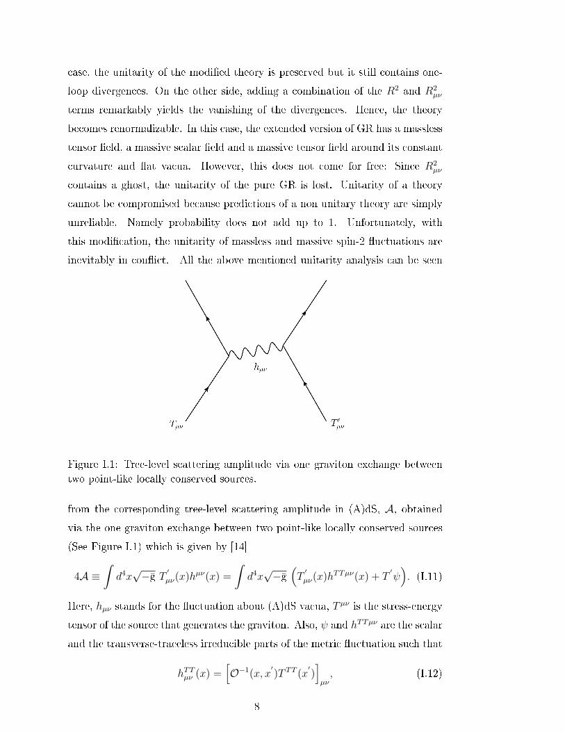
Figure I.1: Tree-level scattering amplitude via one graviton exchange betweentwo point-like locally conserved sources.
from the corresponding tree-level scattering amplitude in (A)dS, A, obtainedvia the one graviton exchange between two point-like locally conserved sources
(See Figure I.1) which is given by [14]
4A ≡∫d4x√−g T ′µν(x)hµν(x) =
∫d4x√−g
(T′
µν(x)hTTµν(x) + T′ψ). (I.11)
Here, hµν stands for the uctuation about (A)dS vacua, T µν is the stress-energy
tensor of the source that generates the graviton. Also, ψ and hTTµν are the scalar
and the transverse-traceless irreducible parts of the metric uctuation such that
hTTµν (x) =[O−1(x, x
′)T TT (x
′)]µν, (I.12)
8
O−1 is the corresponding retarded Green's function obtained from the lineariza-
tion of the corresponding eld equations in the imposed condition ∇µhµν−∇νh =
0. In these higher derivative theories, many classical properties of GR are intact.
For example, just like the ADM conserved quantities of GR [15, 16, 17], con-
served charges can be constructed by using the Killing vectors and these charges
are known as Abbott-Deser-Tekin (ADT) charge and super-potential [18, 19].
I.1.0.1 New Massive Gravity: A Three Dimensional Theory
As mentioned above, due to the conict between the massless and massive spin-
2 modes, GR augmented with the quadratic curvature terms inevitably results
in the violation of the unitarity. On the other hand, since pure GR does not
propagate any dynamical degree of freedom in 3-dimensions, one can study GR
in lower dimensions to better understand the nature of quantum gravity. In
fact there is a vast literature on 3-dimensional gravity [20, 21, 22]. In this aspect,
in 2009, a massive gravity theory called " New Massive Gravity4", was proposed
[23]. The theory, which comes with a particular combination of the quadratic
curvature terms, is given by the action
SNMG =1
κ2
∫d3x√−g[σR− 2λm2 +
1
m2(R2
µν −3
8R2)], (I.13)
where κ2 is the 3-dimensional Newton's constant, λm2 is the cosmological con-
stant and m2 is mass of the graviton. Furthermore, σ is a dimensionless pa-
rameter which can be set to ±1 depending on the unitarity region. With the
specic combination of higher-order terms, the spin-0 mode, that comes from
the addition of R2 term, also drops. And this happens only in 3 dimensions.
Furthermore, at the tree-level, (I.13) has a unitary massive graviton with two
helicities (±2) around both its (A)dS and at vacua. In addition to this, the
model supplies a non-linear extension of the famous massive gravity theory of
4 In 3 dimensions, there is an alternative and unique parity non invariant theory called Topo-
logically Massive Gravity which has a unitary massive graviton with a single helicity [24]. See also a
critical extension of Topologically Massive Gravity dubbed Chiral Gravity [25] which may provide a
well-behaved 3-dimensional quantum gravity theory in asymptotically AdS3 background via Anti-de
Sitter/Conformal Field Theory (AdS/CFT) correspondence.
9
Fierz-Pauli [26] that is dened by the action
SFP =
∫dnx√−g[ 1
κ2R−
m2graviton
2(h2
µν − h2)], (I.14)
which propagates with a massive graviton with 2 degrees of freedom in 3 dimen-
sions and 5 degrees of freedom in 4 dimensions. However, the theory violates
gauge-invariance and also there occurs one more degree of freedom at the non-
linear level which is called the Boulware-Deser ghost [27]. Meanwhile, the
limit m2graviton → 0 is disconnected from the massless case m2
graviton = 0 which is
called the van Dam-Veltman-Zakharov (vDVZ) discontinuity [28, 29]. Only in
3 dimensions Fierz-Pauli theory has a nonlinear extension (with a single eld)
that is the New Massive Gravity theory. On the other side, despite the common
expectation, New Massive Gravity fails to be a renormalizable theory [30, 31].
But if one drops the Einstein term, it might be renormalizable [32]. In addi-
tion to this, it also fails to be a well-dened theory in the context of AdS/CFT
correspondence because the unitarity of bulk and boundary are in conict [23].
Finally, Born-Infeld gravity, an innite order extension of New Massive Gravity
was constructed in [33] which reduces to the ordinary New Massive Gravity in
the quadratic expansion of curvature.
I.2 Conformal Invariance
As it is known, GR has local Lorentz−invariance, general covariance or
dieomorphism−invariance as symmetries5. Although pure GR does not have
conformal symmetry at all, since it preserves the casual structure of spacetimes
up to a conformal factor, let us briey review the basics of conformal trans-
formations in GR: As it is known light-cones of spacetimes remain invariant
up to a conformal factor of the metric, which provides one to demonstrate the
global structures of the spacetime manifolds on a 2-dimensional surface of a pa-
per called Conformal (Penrose) diagrams. This can be seen by observing that,
in n = 4, the metric has 10 independent components. From the energy and
momentum constraints, this reduces to 6. Assuming a light-cone with a spe-
cic coordinate system brings 5 constraints, hence, there remains 1 independent5 In this part, we mainly follow [34].
10

component that allows the invariance of the null-cone structures throughout the
scales a conformal factor of metric [35]. On the other hand, let us review how
conformal symmetry is augmented to GR: Generically, the conformal symmetry
is known as the transformations that preserve the angle between the curves on a
given manifold. Algebraically, under local conformal transformations, the metric
transforms as
gµν → g′
µν = Ω2gµν , (I.15)
where Ω is an arbitrary function of coordinates but we assume Ω > 0. Moreover,
using (I.15), one can show that the Christoel connection transforms as
Γαµν → Γ′αµν = Γαµν + Ω−1(δαν∇µΩ + δαµ∇νΩ− gµν∇αΩ). (I.16)
Therefore, from (I.16) and the denition of Riemann tensor
Rµνρσ = ∂ρΓ
µνσ − ∂σΓµνρ + ΓµλρΓ
λνσ − ΓµλσΓλνρ, (I.17)
one can easily show that, under (I.15), the Riemann tensor transforms according
to
Rµνρσ → R
′µνρσ = Rµ
νρσ+Ω−2[gνσ(
2∇ρΩ∇µΩ− Ω∇ρ∇µΩ)
+ δµσ
(Ω∇ν∇ρΩ− 2∇νΩ∇ρΩ + gνρ∇αΩ∇αΩ
)− gνρ
(2∇σΩ∇µΩ− Ω∇σ∇µΩ
)− δµρ
(Ω∇ν∇σΩ− 2∇νΩ∇σΩ + gνσ∇αΩ∇αΩ
)].
(I.18)
Contracting (I.18) yields the transformation of Ricci tensor as
Rµν → R′
µν = Rµν + Ω−2[(n− 2)(2∇µΩ∇νΩ− Ω∇ν∇µΩ)
− gµν(
(n− 3)∇αΩ∇αΩ + ΩΩ)],
(I.19)
where ≡ ∇α∇α. Finally, the conformal transformation of the Ricci scalar
reads
R→ R′= Ω−2
[R− (n− 1)Ω−2
((n− 4)∇αΩ∇αΩ + 2ΩΩ
)]. (I.20)
Hence, with these transformations, one will nally obtain the conformal trans-
formation of the Einstein tensor as
Gµν → G′
µν = Gµν + (n− 2)Ω−2[2∇µΩ∇νΩ− Ω∇ν∇µΩ
+ gµν((n− 5)
2∇αΩ∇αΩ + ΩΩ
)].
(I.21)
11
Of course by using the above transformations of the curvature terms, one can
study the conformal extension of any given gravity model. Alternatively, by
using the experience of making a global symmetry local with the help of extra
elds, one can modify GR and other extensions of it as gauge theories such that
they will recover the above mentioned conformal transformations for the specic
choices of elds. As we will see in detail in the next chapters, one such (in fact
the rst attempt) was done by Weyl in 1918 [36] in order to unify electromagnetic
theory and gravity via a real scalar and an Abelian gauge elds.
I.3 Spontaneous Symmetry Breaking
In Quantum Field Theory perspective, elementary particles are labeled via their
masses and their spins. This was worked out long time ago by Wigner [37].
Furthermore, this unique framework also gives what values of these labels can
be: According to Quantum Field Theory in at space, due to the requirements
of unitarity, the masses of the particles in the subatomic world are not allowed
to be negative, and additionally their spins can only be 0, 12, 1, 3
2in units of ~.
Note that Wigner's theorem allows higher spins but in four dimensions, one
cannot have a renormalizable interacting eld theory for spins larger than 32~.
In this construction, all the matter particles (i.e., fermions) quarks, electron,
muon, tau have m2 ≥ 0 and spin-12. Also, the force carriers (i.e., bosons) of the
Electrodynamic and Strong interactions (photon and gluons, respectively) have
m2 = 0 and spin-1 with two degrees of freedom. On the other side, even though
the mediators of the Weak Interaction (i.e. W±, Z bosons) have spin-1, in
contrary to the photon and gluons, they are massive with values approximately
90 times the proton mass and receive an extra third degree of freedom. Then, a
natural question inevitably arises: what kind of a process causes the generation
of these masses and hence the existence of this additional degree of freedom?
At the time, this had been a really subtle issue until the Higgs mechanism was
proposed [38]. In this mechanism, it is stated that the masses and hence the
above mentioned third degrees of freedom of the mediators of the Electroweak
12

interaction are generated via the spontaneous breaking6 of the corresponding
local SU(2)×U(1) gauge symmetry to U(1) in the classical vacuum of the Higgs
potential given in the Figure I.2. So electromagnetism becomes an eective U(1)
theory.
Figure I.2: Mexican-hat-like Higgs Potential.
As it is known, the Higgs potential that provides the breaking of the symmetry
is somehow a hard one. That is to say, it is put in the Lagrangian of the
Higgs eld by hand. At that step, one can ask what actually stays behind this
spontaneous symmetry breaking without assuming a potential whose classical
solution has a nonzero value? That is, one would like to have such a mechanism
that will provide the existence of the spontaneous breaking of the continuous
symmetry which automatically arises from the nature of theory. This important
question was answered by Coleman and Weinberg in 1973 [39]. In their paper,
using the functional method, after a regularization and renormalization process,
they showed that the radiative corrections at the one-loop level to the eective
potential for the Φ4-theory remarkably changes the minimum at the origin into
a maximum, and hence shifts this minimum to a nonzero point which automat-
ically induces the spontaneous symmetry breaking. That is to say, they proved
that the higher-order corrections due to the self-interactions are in fact the back-
bone of the spontaneous breaking of the symmetry. Unfortunately, Coleman and
Weinberg mechanism could not explain the symmetry breaking mechanism in
6 Here, by symmetry-breaking, it means that although a given action is invariant under a con-
tinuous symmetry, its vacuum is not.
13

the Standard Model, since it gave a very light (4 GeV) Higgs particle. Of course
we now know that the Higgs boson was found with the mass 126 GeV [40].
Therefore, apparently, in the Standard Model, symmetry breaking is not a loop
result but a tree-level result.
As we will see in the next chapters, the Weyl symmetry augmented in the Higher
Derivative Gravity theories is spontaneously broken in (A)dS backgrounds in
analogy with the usual Standard Model Higgs Mechanism, whereas it is radia-
tively broken via Coleman-Weinberg mechanism in the at vacuum. Hence, the
uctuations gain their masses via symmetry breaking. Because of this, let us
now briey review the Higgs and Coleman-Weinberg mechanisms, separately:
I.3.1 Higgs Mechanism
In this part, we will review the basics of the Higgs mechanism by mainly following
[41]: Historically, the idea of symmetry breaking was rst used in superconduc-
tivity in order to explain the generation of Cooper pairs which is known as The
Bardeen-Cooper-Schrieer (BCS) Model [42, 43, 44].
In his paper, Nambu showed that the Goldstone theorem was in fact valid in any
spontaneously broken continuous global symmetry (1960): That is, there would
always occur a massless scalar particle for each broken generator whenever a
continuous global symmetry was broken. Later, the idea of the spontaneous
symmetry breaking was extended to the particle physics by Nambu and Jona-
Lasinio [45] in 1961. In 1963, Anderson introduced the rst but non-relativistic
version of the local spontaneous symmetry breaking by showing that, when the
local symmetry is broken, there does not occur a Nambu-Goldstone boson in
the certain examples of superconductors, rather the vector elds gain masses
[46]. In 1964, Higgs, Englert-Brout and Guralnik-Hagen-Kibble [38] separately
constructed the relativistic version of the Anderson mechanism and it was later
dubbed The Higgs mechanism. Therefore, to be historically consistent, let us
rst review the spontaneous symmetry breaking of a global symmetry briey,
and after that skip to the study of Standard Model Higgs mechanism:
14

Spontaneously Broken Global Symmetry and Generation of Nambu-
Goldstone Bosons
To see what happens when a continuous global symmetry is spontaneously bro-
ken, let us work on the Lagrangian density for a complex scalar eld
L = ∂µΦ∗∂µΦ− λ2
2(ΦΦ∗ − ν2)2, (I.22)
which contains a Mexican-hat-like potential whose vacuum expectation value
(VEV), < φ >, is ν. At it is seen, (I.22) has a global U(1)-invariance. That is,
transforming Φ as
Φ→ Φ′= eiγΦ, (I.23)
leaves (I.22)-invariant with γ real. One should observe that, since the scalar eld
is a complex eld, one can rewrite it in terms of its modulus and a phase factor
as Φ = |Φ|eiσ. Therefore, depending on σ, the theory has innite numbers of
vacua, each of which has the same VEV of ν. Hence, the solutions also have
the global U(1)-invariance, and thus the symmetry remains unbroken. On the
other hand, by freezing σ to any arbitrary constant, the solution will choose
a certain vacuum and so the symmetry will be spontaneously broken. As it is
known, in the Quantum Field Theory context, the particles are interpreted as
the uctuations around the vacuum values of the elds. Therefore, to read the
fundamental excitations propagated about the vacuum in this broken phase, let
us set σ = 0 for simplicity, and expand Φ about its vacuum value as
Φ = ν +1√2
(Φ1 + iΦ2), (I.24)
where Φ1 is the eld normal to the potential that points toward the higher-
values of the potential, whereas Φ2 is the one that horizontally parallels to curve.
Moreover, by plugging (I.24) into (I.22), one will nally nd that the theory has
a massive scalar eld Φ1 with mass mΦ1 =√
2λν and a massless scalar eld
Φ2 dubbed "Nambu-Goldstone boson". To summarize, there always occurs a
massless boson if a continuous global symmetry is spontaneously broken. Since
there are not massless scalar particles in Nature, this spontaneous symmetry
breaking of a global symmetry seems a little irrelevant for particle physics.
15
Spontaneously Broken Local Symmetry: The Higgs Mechanism
In this section, we will study the spontaneous-breaking of the local symmetry
dubbed The Higgs mechanism7. As it is known, local symmetry is implemented
to a theory via gauge vector elds. Since these elds can be either Abelian or
non-Abelian, it will be more convenient if one studies the Higgs mechanism for
these two distinct cases, separately:
Spontaneous Symmetry Breaking in Abelian Gauge Theories
In this part, we analyze the spontaneous symmetry breaking of the local U(1)
symmetry in which the complex scalar eld (or Higgs eld) transforms according
to
Φ→ Φ′= eieσ(x)Φ. (I.25)
In contrary to the global case, by inserting (I.25) into (I.22), one can easily show
that, due to the partial derivatives, there will occur extra terms such that they
will prevent the Lagrangian density to be invariant under (I.25). For this reason,
by using Abelian vector eld, one needs to assume a new derivative operator,
Dµ, called "gauge-covariant derivative", which acts on Φ as
DµΦ = ∂µΦ + ieAµΦ, (I.26)
in order to get rid o the symmetry violating terms. Taking the canonically
normalized kinetic term for the gauge eld into account and replacing the usual
derivative operators in (I.22) with the one in (I.26), one will get
L = (DµΦ)∗DµΦ− λ2
2(ΦΦ∗ − ν2)2 − 1
4FµνF
µν , (I.27)
where Fµν = ∂µAν − ∂νAµ is the eld-strength tensor for the vector elds. Note
that, with this modication, the theory gains local U(1)-invariance, with Aµ
transforms as Aµ → A′µ = Aµ − ∂µσ(x). Let us now rewrite the Higgs eld in
terms of its modulus and phase as
Φ = |Φ|eiγ(x) =(ν +
1√2ψ(x)
)eiγ(x). (I.28)
7 The mechanism is sometimes called Anderson-Higgs mechanism, since Anderson made the
rst observation that photon becomes eectively massive in a superconductor via this mechanism.
16

Here the modulus was also expanded about the vacuum. Furthermore, as in the
global case, by freezing γ(x) to zero, one will x the gauge-freedom, and will
be left with the real eld. Thus, xing the gauge-freedom spontaneously breaks
the local symmetry. To read the fundamental excitations about the vacuum,
by inserting (I.28) into (I.27), one will nally see that the theory has a massive
scalar eld with mass mψ =√
2λν and a massive vector eld with the mass
mAµ =√
2|e|ν. However, in this case, the Nambu-Goldstone boson does not
exist. One often says that the Nambu-Goldstone boson is eaten by the massive
vector eld. Thus, the mechanism provides a way to give masses to the gauge
particles as is desired in the weak sector of the Standard Model. In this example,
the scalar eld becomes the third degree of freedom for the massive photon.
Spontaneous Symmetry Breaking in non-Abelian Gauge Theories
It is known that, in its unbroken phase, the Electroweak theory is invariant
under the local SU(2) × U(1) gauge group. Here in this case, the Higgs eld
is a doublet (i.e., composing of two complex parts) and transforms according
to the fundamental representation of the group. Let us study how this local
symmetry is augmented to the theory: As in the previous part, due to the extra
terms coming from the usual partial derivatives, one should replace the usual
derivative operator with a proper gauge-covariant derivative, Dµ. But here, Dµmust be composed of the gauge elds belonging to both SU(2) and U(1). More
precisely, by dening the non-Abelian gauge eld to be Aµ (a matrix) of SU(2)
and Abelian gauge eld to be Bµ (a function) of U(1), one can dene
DµΦ = ∂µΦ− ifσaAaµΦ− if ′eBµΦ. (I.29)
Here, σa; a = 1, 2, 3, are the generators of the SU(2) gauge group (i.e., Pauli
spin matrices)8 and f , f′are the coupling constants of the gauge elds . There-
fore, locally SU(2) × U(1)-invariant Lagrangian density of the Higgs eld and
the vector elds becomes
L = (DµΦ)+DµΦ− λ2
2(ΦΦ∗ − ν2)2 − 1
4F aµνF
aµν − 1
4FµνF
µν , (I.30)
8 Note that the non-Abelian gauge eld Aµ is expanded in the generator basis of the SU(2)
group with the coecient Aaµ.
17
where F aµν = ∂µA
aν − ∂νA
aµ + fεabcAbµA
cν and Fµν = ∂µBν − ∂νBµ. Note that
−1/4 are chosen in order to have canonically normalized kinetic terms for the
gauge elds. As in the Abelian case, here, one can eliminate 3 components of
the Higgs eld via xing the gauge-freedom and arrives at
Φ = ν +1√2ψ, (I.31)
which hence spontaneously breaks SU(2)×U(1)-symmetry into U(1). Moreover,
in order to obtain the fundamental excitations and their masses, let us dene
σ+ =1√2
(σ1 + iσ2), σ− =1√2
(σ1 − iσ2), (I.32)
which yields
A±µ =1√2
(A1µ ± iA2
µ). (I.33)
Hence, one will obtain
σaAaµ = σ+A−µ + σ−A+µ + σ3A3
µ. (I.34)
Then, by substituting (I.34) into (I.30), one will nally get
mZ =1√2νf , mW =
1√2νf, (I.35)
where
f = (f 2 + f′2)1/2,
f
f= cos θW ,
f′
f= sin θW . (I.36)
Here θW is called Weinberg angle which is ∼ 29.3137 ± 0.0872. Finally, the
massless photon will be dened by the transverse component
Aµ = A3µ sin θW +Bµ cos θW . (I.37)
This corresponds to the unbroken U(1) symmetry.
I.3.2 Coleman-Weinberg Mechanism in n = 4 and n = 3 Dimensions
In the Standard Model Higgs mechanism, the spontaneous symmetry breaking
of the local gauge symmetry is via the nonzero classical vacuum expectation
value of the Higgs eld. The crucial thing is that, at the Lagrangian level, it is
assumed that the complex scalar eld has a potential that provides symmetry-
breaking. Naturally, one can search for a mechanism that will automatically give
18
such a symmetry breaking without adding any hard symmetry breaking term.
The question was answered by Coleman and Weinberg in 1973 [39]: Using the
electrodynamics of charged massless scalar eld, they showed that, even though
the minimum of the interaction potential is zero at the tree-level, the higher-
order corrections at the one loop level to the eective potential convert the
shape of the potential into a Mexican-hat-type one by turning the minimum at
the origin into a maximum. Therefore, the minimum is shifted to a nonzero
point which breaks the symmetry spontaneously. In this part, we will review
the Coleman-Weinberg calculations for the renormalizable scalar potential Φ4
in n = 4 dimensions [39] and its 3−dimensional version known as Tan-Tekin-
Hosotani computations for the two-loop radiative corrections to the eective-
potential for the Φ6 interactions [47]:
As mentioned above, Coleman and Weinberg used the scalar eld Lagrangian
density
L = −1
4FµνF
µν +1
2(∂µΦ1 − eAµΦ2)2 +
1
2(∂µΦ2 − eAµΦ1)2
− µ2
2(Φ2
1 + Φ22)− λ
4!(Φ2
1 + Φ22)2 + counter terms,
(I.38)
in order to study the eect of higher-order corrections to the eective poten-
tial9. Note that a compact form of counter-terms are also inserted in (I.38)
which are generically done in Quantum Field Theory in order to absorb the
singularities that arise during the regularization and renormalization procedure.
It is known that, when bare mass scale µ2 ≥ 0, (I.38) becomes a usual stable
Quantum Field Theory which propagates with a charged massive scalar and its
massive anti-particle particle and a massless photon. On the other hand, when
µ2 < 0, the vacuum Φ1 = Φ2 = 0 is unstable and the symmetry is spontaneously
broken. In this case, the theory propagates with a massive neutral scalar and a
massive vector particles. For the second case, the crucial question is whether the
occurring symmetry breaking is due to the negativity of µ2 or actually due to
higher-corrections in the potential? And the more important question is what
would happen when µ2 = 0, namely when the theory is massless classically?
In [39], as we will see below, it was shown that symmetry breaking is actually
9 The decomposition of Φ = Φ1 + iΦ2 is used in (I.38).
19
because of the radiative corrections coming from the self-interactions of elds
when µ2 = 0. In their approach, there also occurs an interesting result dubbed
dimensional transmutation that roughly stands for the change in relations be-
tween dimensionless parameters as well as the generation of dimensionful ones
via radiative corrections: More precisely, when µ2 = 0, the action contains two
independent dimensionless parameters e and λ. Surprisingly, after the one-loop
calculations are carried out, these two distinct parameters depend on each other
[i.e., λ = λ(e)] and a dimensionful parameter that is the vacuum expectation
value of the scalar eld, which provides the spontaneous symmetry breaking,
comes into the picture. Therefore before the symmetry breaking one has two
dimensionless parameters and after the symmetry breaking one has one dimen-
sionful and one dimensionless parameter; hence the dimensional transmutation.
As it is known, the structure of eective potential directly determines what
kind of symmetry breaking process will occur. However, computations for the
eective potential generically is really a subtle task because one has to compute
and collect innite number of diagrams in order to nd the potential. One
of the leading procedures is the loop expansion method in which one nds the
contributions coming from each separate part of the diagrams order by order (i.e.,
starting from tree-level to r-loops) and then sum them to nd the desired result
for the eective potential10. The procedure that was followed is the functional
method [48] which was extended in study of spontaneous symmetry breaking in
[49]: To see how this method works, let us suppose that the Lagrangian density
for the scalar eld is replaced with the one that includes a source
L(Φ, ∂µΦ)→ L′(Φ, ∂µΦ) ≡ L(Φ, ∂µΦ) + J (x)Φ(x). (I.40)
The functional W which gives all the connected Feynman diagrams is dened
10 By assuming an overall dimensionless parameter a such that
L → L′≡ a−1L, (I.39)
one can show that the loop expansion procedure corresponds to the power-series expansion of a, which
is , at the end, freezed to 1. Needless to say that because of being an overall parameter, a does not
change the physical results rather it controls the expansion. The advantage of the r-loop expansion
method is that it provides all the vacua of the theory simultaneously (For the detailed proof and
discussion see [39].)
20
as
eiW = 〈0future|0past〉, (I.41)
namely it is the vacuum to vacuum transition amplitude. The functional can
also be expressed in terms of the sources as
W(J ) =∑r
1
r!
∫d4x1 . . . d
4xrO(r)(x1 . . . xr)J (x1) . . .J (xr), (I.42)
where Or is the propagator that gives the sum of all the connected diagrams
with r external legs. Furthermore, the classical solution is dened by
Φc(x) =δWδJ (x)
=〈0future|Φ(x)|0past〉〈0future|0past〉
∣∣∣∣J=0
, (I.43)
which provides one to dene an eective action Γ(Φc) as a Legendre transfor-
mation
Γ(Φc) =W(J )−∫d4xJ (x)Φc(x). (I.44)
Observe that the variation of the action with respect to the classical solution
givesδΓ
δΦc(x)= −J (x). (I.45)
Similarly, the eective action can also be written as
Γ(Φc) =∑r
1
r!
∫d4x1 . . . d
4xr ∆(r)(x1 . . . xr)Φc(x1) . . .Φc(xr). (I.46)
Here, ∆(r) is the propagator that gives all the one-point-irreducible (1PI) dia-
grams with r-external legs that cannot be disconnected by cutting any internal
line. Even though 1PIs contain external legs, their propagators do not contain
any contribution coming from these legs. Alternatively, one can also express the
eective action in terms of the potentials as
Γ =
∫d4x
(− V(Φc) +
1
2(∂µΦc)
2Z(Φc) + . . .), (I.47)
where V is "the eective potential" whose r-times derivatives give all the loops
which are only composed of 1PIs diagrams with vanishing momentums of exter-
nal legs. Thus, the renormalization conditions due to the perturbative expansion
near the origin can be expressed as follows: When one wants the operator cor-
responding to the propagator to be zero at the external lines, one should set
µ2 =d2VdΦ2
c
∣∣∣∣Φc=0
. (I.48)
21
Meanwhile, requiring the four-point function at the external legs to be the di-
mensionless coupling constant λ yields
λ =d4VdΦ4
c
∣∣∣∣Φc=0
. (I.49)
And nally, one should normalize the wave-function as
Z(Φc = 0) = 1. (I.50)
To see how eective potential of a given theory is explicitly evaluated via one-
loop correction using the functional method, it is more pedagogical to work on
a simpler example: For this purpose, let us consider the Lagrangian density of
the complex scalar eld that interacts via Φ4
L =1
2(∂µΦ)∗∂µΦ− λ
4!Φ4 +
α
2(∂µΦ)∗∂µΦ− β
2Φ2 − γ
4!Φ4. (I.51)
Here, α, β and γ are the bare counter-terms of the wave-function, mass and
coupling constant which will eat the singularities at the end. As it is seen, one
will read the tree-level potential
V =λ
4!Φ4c . (I.52)
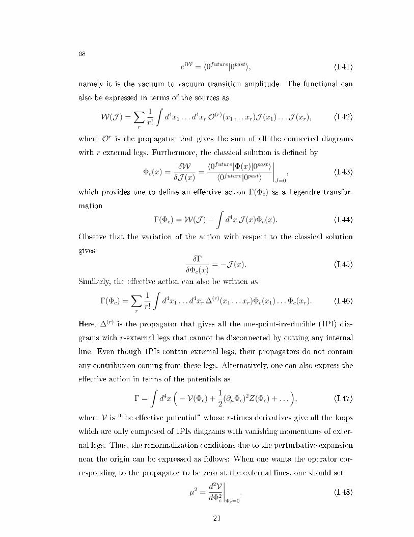
Figure I.3: One-loop corrections resulted from the sum of innitely numbers ofquartically self-interacting scalar elds.
On the other side, due to the innite number of the one-loop diagrams, the ef-
fective potential will not be obvious. Hence, by adding the contributions coming
22
from the counter-terms and using the eective action obtained above, one will
obtain the total eective potential at the one-loop level (Figure I.3) as
V =λ
4!Φ4c −
β
2Φ2c −
γ
4!Φ4c + i
∫d4k
(2π)4
∞∑r=1
1
2r
( λ2Φ2c
k2 + iε
)r. (I.53)
Here, i is due to the generating functional W of the connected diagrams. Also,
1/2 is substituted since we have bosons. Moreover, since the change of any two
external legs at the same vertex does not bring any new diagram, we plugged
1/4! in the numerator which cancels the ordinary one. Finally, since any r-
face diagram is invariant under reection and rotation, the 1/n! is also inserted
which eliminates the one coming during expansion. Collecting the series as well
as using Wick-rotation (i.e., replacing k0 with ik0), one will nally reach
V =λ
4!Φ4c −
β
2Φ2c −
γ
4!Φ4c +
1
2
∫d4k
(2π)4ln
(1 +
λΦ2c
2k2
). (I.54)
One should observe that the power-counting yields that the integral diverges as
k → 0 and as k → ∞. Therefore, (I.54) is in fact both IR and UV-divergent.
To cure the UV-divergence, one can assume a cut-o scale Λ in (I.54) such that
it will give
V =λ
4!Φ4c +
β
2Φ2c +
γ
4!Φ4c +
λΛ2
64π2Φ2c +
λ2Φ4c
256π2
[ln(λΦ2
c
2Λ2
)− 1
2
], (I.55)
where all the terms that disappear as Λ → ∞ were not taken into account.
Hereafter, one needs to nd the explicit values of the counter-terms: This can
be reached via the requirements of the renormalized mass and coupling-constant:
First of all, the renormalized mass is expected to be zero which then converts
the rst renormalization condition (I.48) into
µ2 =d2VdΦ2
c
∣∣∣∣Φc=0
= 0, (I.56)
that yields
β = − λΛ2
32π2. (I.57)
However, due to the IR-divergence at the origin, one cannot evaluate the renor-
malized coupling constant via the above dened second renormalization condi-
tion (I.49). In momentum space, the coupling-constants cannot be evaluated at
the on-shell mass point because it stays at the top of the IR-divergence. The
23
cure is that one needs to evaluate the coupling-constants at an arbitrary non
zero point M which is far from the on-shell singular-point. In another words,
one can assume the renormalized coupling constant to be
λ =d4VdΦ4
c
∣∣∣∣Φc=M
, (I.58)
which induces the renormalized wave function counter-term to be Z(M) = 1.
Hence, (I.58) will nally become
γ = − 3λ2
32π2
[ln(λM2
2Λ2
)+
11
3
]. (I.59)
Thus, by collecting all these results, one will nally obtain the eective potential
at the one-loop level as
V =λ
4!Φ4c +
λ2Φ4c
256π2
[ln( Φ2
c
M2
)− 25
6
]. (I.60)
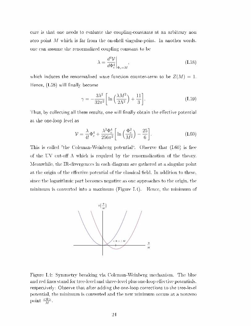
This is called the Coleman-Weinberg potential. Observe that (I.60) is free
of the UV cut-o Λ which is required by the renormalization of the theory.
Meanwhile, the IR-divergences in each diagram are gathered at a singular point
at the origin of the eective potential of the classical eld. In addition to these,
since the logarithmic part becomes negative as one approaches to the origin, the
minimum is converted into a maximum (Figure I.4). Hence, the minimum of
Figure I.4: Symmetry breaking via Coleman-Weinberg mechanism. The blueand red lines stand for tree-level and three-level plus one-loop eective potentials,respectively: Observe that after adding the one-loop corrections to the tree-levelpotential, the minimum is converted and the new minimum occurs at a nonzeropoint <Φ>
M.
24
the potential is shifted to a nonzero point
lnΦc
M= −16π2
3λ. (I.61)
Thus, the symmetry is spontaneously broken11. But actually it turns out that
in this new minimum the perturbation theory breaks down as the renormalized
mass scale µ2 (and hence the renormalized coupling constant λ) receives greater
values, which is then cured when one takes into account the one-loop corrections
of the gauge eld part [39]. Finally, one can easily show that the arbitrary
renormalized mass parameter M does not play any role in the physical results.
For instance, by assuming another renormalized point M , then, the eective
potential at the one-loop level will turn into
V =λ
4!Φ4c +
λ2Φ4c
256π2
[ln( Φ2
c
M2
)− 25
6
]+O(λ3). (I.62)
Hence, M is nothing but a parametrization of same potential at the given order.
Actually, any change in the renormalized coupling constant (I.58) and the scale
of the eld Z(M) = 1 will induce a proper change in the renormalized mass M
whose (and so of the coupling constant) exact region at a given energy scale is
determined via the "renormalization group ow" given by [50][M
∂
∂M+ η
∂
∂λ+ ζ
∫d4xΦc(x)
δ
δΦc(x)
]Γ = 0, (I.63)
where η and ζ are parameters that depend on λ. By using (I.46), (I.63) turns
into [M
∂
∂M+ η
∂
∂λ+ rζ
]Γr(x1 . . . xr) = 0. (I.64)
Using (I.47), one will obtain[M
∂
∂M+η
∂
∂λ+ζΦc
∂
∂Φc
]V = 0,
[M
∂
∂M+η
∂
∂λ+ζΦc
∂
∂Φc
+2ζ
]Z = 0. (I.65)
Since it is more useful to work with the dimensionless parameters that generically
rely only on the ratio Φc/M , by dening the following dimensionless functions
V(4) =∂4V∂Φ4
c
, t = ln(Φc
M), η =
η
1− ζ, ζ =
ζ
1− ζ, (I.66)
11 One might also think that the r-loop corrections beyond the one-loop level may convert this
maximum again into a minimum. In fact this is partially true, that is if such a situation takes place,
then this higher order corrections to the eective potential will just result in local minima. That is
to say, since the contributions coming from the higher orders will always be smaller than the one
coming from the one-loop computation, they will not turn this maximum into an absolute minimum,
but rather they will only cause a local tilted minima at the top of this overall maximum [39].
25
one will be able to convert (I.65) into a fully-dimensionless ow equations[− ∂
∂t+ η
∂
∂λ+ 4ζ
]V(4)(t, λ) = 0,
[− ∂
∂t+ η
∂
∂λ+ 2ζ
]Z(t, λ) = 0. (I.67)
Moreover, with these redenitions, the conditions above mentioned can also be
written as
V(4)(0, λ) = λ, Z(0, λ) = 1. (I.68)
Hence, using (I.68) in (I.67) yields the ow coecients as
ζ =1
2∂tZ(0, λ), η = ∂tV(4)(0, λ)− 4ζλ. (I.69)
Therefore, the renormalization group ow coecients can be evaluated as long
as the time derivatives of the conditions (I.68) are known. However, even though
the loop expansions of those derivatives will bring important results, their exact
form are not known. To cure this subtle issue, let us suppose that the ow
coecients are completely known which provide us to assume a general ow
equation [− ∂
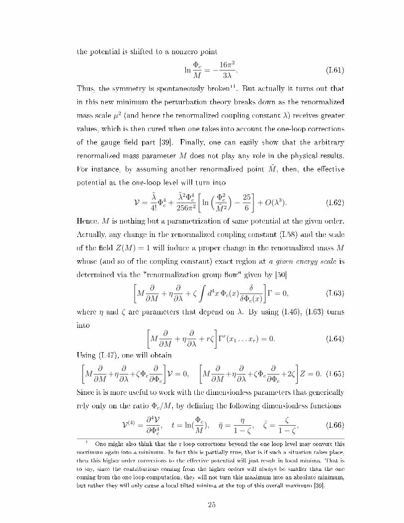
∂t+ η
∂
∂λ+ 4ζ
]F(t, λ) = 0, (I.70)
that covers (I.65). The current aim is to nd a generic renormalized coupling
constant λ′(which at t = 0 reduces to λ) such that
η(λ′) =
dλ′
dt. (I.71)
Thus, one will get the solution of (I.69) as
F(t, λ) = h[λ′(t, λ)]en
∫ t0 dt′ζ[λ′(t′,λ)]. (I.72)
Here h is an arbitrary function depends on λ′that is freezed by the ow coe-
cients (I.68) as
Z(t, λ) = e2∫ t0 dt′ζ[λ′(t′,λ)], V(4)(t, λ) = λ
′(t, λ)[Z(t, λ)]2. (I.73)
Thus, intervals for the renormalized conditions are exactly determined in terms
of the derivatives of renormalization group ow coecients η and ζ. Now, by us-
ing t = ln(ΦcM
), dierentiating the one-loop eective Coleman-Weinberg potential
(I.60) with respect to Φc gives
V(4) = λ+3λ2t
16π2. (I.74)
26

Furthermore, substituting (I.74) into the second equation of (I.69) yields
η =3λ2
16π2. (I.75)
Thus using (I.71), one will nally arrive at
λ′=
λ
1− 3λt16π2
, V(4) =λ
1− 3λt16π2
. (I.76)
Thus, the one-loop corrections to the eective potential is valid when |λ| 1
and |λt| 1 [39].
This pure scalar eld example was unrealistic but gave us an example calculation
of the Coleman-Weinberg Potential. By following the same steps given above
and taking into account the one-loop diagrams of the photon12, one will nally
obtain the one-loop eective potential for the charged massless scalar meson
coupled to U(1)-gauge eld which is dened by the action (I.38) as
V =λ
4!Φ4c +
3e4Φ4c
64π2
[ln( Φ2
c
〈Φ〉2)− 25
6
], (I.77)
where 〈Φ〉 is minimum of the one-loop eective potential. Furthermore, by
taking the derivative of V with respect to Φc, one will arrive at an interesting
result
λ =33
8π2e4. (I.78)
Thus, in broken phase, dimensionless constants become related and with the
generation of the nonzero vacuum expectation of the scalar eld, one has a
"dimensional transmutation" as explained above. Following the same steps given
in the renormalization group ow part, one will obtain
ζ =3e2
16π2, η =
5λ2
6− 3e2λ+ 9e4
4π2, (I.79)
which will give the corresponding domains of the parameters as
e′2 =
e2
1− e2t24π2
, λ′=e′2
10
[√719 tan
(1
2
√719 ln e
′2 + θ)
+ 19
], (I.80)
where θ is the integration constant determined via the requirements of λ′
= λ
and e′= e.
12 Here, due to the minimal coupling between the scalar eld and the gauge eld, there will also
occur similar one-loops diagrams for the photon [39].
27

Finally, the 3-dimensional Coleman-Weinberg-like calculations to the eective
potential was evaluated by P.N. Tan, B. Tekin, and Y. Hosotani in 1996-1997
[47]. They computed the eective potential at the two-loop level for the Maxwell-
Chern-Simons charged scalar Electrodynamics, which self-interacts through the
Φ6-couplings, given by
L = −a4FµνF
µν − κ
2εµνρAµ∂νAρ + L(G.F.) + L(F.P )
+1
2(∂µΦ1 − eAµΦ2)2 +
1
2(∂µΦ2 + eAµΦ1)2
− m2
2(Φ2
1 + Φ22)− λ
4!(Φ2
1 + Φ22)2 − ν
6!(Φ2
1 + Φ22)3,
(I.81)
where L(G.F.) and L(F.P ) are the related gauge-xing term (in t'Hooft-gauge) and
Faddeev-Popov ghost
L(G.F.) = − 1
2ξ(∂µA
µ − ξeηΦ2)2, L(F.P ) = −c+(∂2 + ξe2ηΦ1)c. (I.82)
Referring to [47] for the details of the calculations, after a long regularization
and renormalization computations, one gets the the one-loop eective potential
in the Landau gauge (ξ = 0) for the full theory (I.81) as
V 1−loopeff (ν) =
ν
6!ν6 +
~12π
e6
a3F(x), (I.83)
where
F(x) = 3κx2 − (κ2 + 4x2)1/2(κ2 + x2) +2κ4(240M2 − 62Mκ2 + κ4)
(4M + κ2)11/2x6
+ κ3,
(I.84)
and
x =
√aν
e, M =
aM
e2, κ =
κ
e2. (I.85)
When M = 0 and κ 6= 0, then F ≥ 0 thus the overall minimum at the origin
is not altered, thus the U(1) symmetry remains unbroken. On the other hand,
for the choice of M = κ2, then one will get F(x)/κ3 = 3y2 − (1 + 4y2)1/2(1 +
y2) + 0.00512y2 + 1, the minimum occurs at a nonzero point away from the
origin; hence the symmetry is spontaneously broken. If κ = 0, then the second
renormalization condition for the coupling constant fails. Therefore, by imposing
the renormalization scale to be M1/2, then one can see that the minimum also
occurs at a nonzero point so the symmetry breaking takes place. Thus, due
28
to this, one should go beyond one-loop in order to explicitly determine the
corresponding symmetry-breaking.
To nd the two-loop corrections to the eective potential, one needs to determine
the fundamental graphs in the full theory. There are in fact ve types of the
graphs whose two-loop corrections to the eective potentials quoted from [47]
are
1. Two scalar loops: The two-loop eective potential due to the two scalar
loops is found
V(q1)eff =
~2
(4π)2
3( λ
4!+
15νv2
6!
)m2
1+3( λ
4!+
3νv2
6!
)m2
2
+ 2( λ
4!+
9νv2
6!
)m1m2
.
(I.86)
Figure I.5: Two scalar loops.
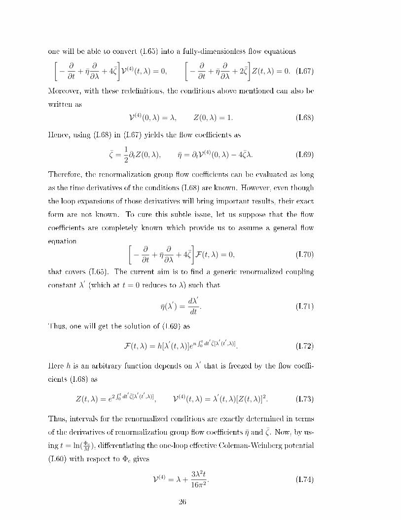
2. One scalar and one gauge loop: The two-loop eective potential due to
the one scalar and one gauge loop is
V(q2)eff =
e2~2
16π2a
(m1 +m2)(m2+ +m2
−)
m+ +m−. (I.87)
Figure I.6: One scalar and one gauge loop.
29

3. θ-shape diagram: The two-loop eective potential due to the θ-shape dia-
gram is found
V(c1)eff = − ~2
32π2
3( λ
3!ν +
ν
36ν3)2
+( λ
3!ν +
ν
60ν3)2
×− 1
n− 3− γE + 1 + ln 4π
+
~2
32π2
3( λ
3!ν +
ν
36ν3)2
ln(3m1)2
µ2
+( λ
3!ν +
ν
60ν3)2
ln(m1 + 2m2)2
µ2
.
(I.88)
Figure I.7: θ-shape diagram.
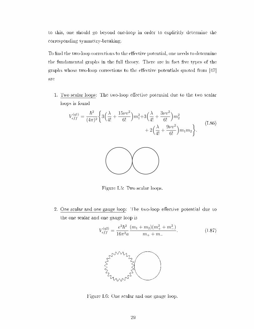
4. θ-shape diagram with two scalar and one gauge propagators: The corre-
30
sponding two-loop eective potential is found
V(c2)eff =
~2e2
64π2a
[2(m2
1 +m22)− (m+ +m−)2 + 3m2
3
]×[− 1
n− 3− γE + 1 + ln 4π
]+ 2
[m1m2 −
(m1 +m2)[2(m1 −m2)2 +m2+ +m2
−]
m+ +m−
]− (m2
1 −m22)2
m23
ln(m1 +m2)2
µ2
−∑a=±
2m2a(m
21 +m2
2)−m4a − (m2
1 −m22)2
ma(m+ +m−)ln
(ma +m1 +m2)2
µ2
− 5
6
κ2
a2
.
(I.89)
Figure I.8: θ-shape diagram with two scalar and one gauge propagators.
5. θ-shape diagram with two gauge and one scalar propagators: The corre-
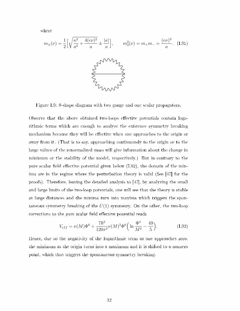
sponding two-loop eective potential is found
V(c3)eff = −3~2e2ν2
64π2a2×− 1
n− 3− γE + 1 + ln 4π
− ~2e4ν2
32π2a2
− 2m1
m+ +m−− 2m2
1 + 12m23
(m+ +m−)2+ 3
+
~2e4ν2
128π2a2
2[(m+ −m−)2 −m2
1]2
m23(m+ +m−)2
ln(m+ +m− +m1)2
µ2
+m4
1
m43
lnm2
1
µ2
+∑a=±
[(4m2
a −m21)2
m2a(m+ +m−)2
ln(2ma +m1)2
µ2
− 2(m2a −m2
1)2
m23ma(m+ +m−)
ln(ma +m1)2
µ2
],
(I.90)
31
where
m±(ν) =1
2
[√κ2
a2+
4(eν)2
a± |κ|
a
], m2
3(ν) = m+m− =(eν)2
a. (I.91)
Figure I.9: θ-shape diagram with two gauge and one scalar propagators.
Observe that the above obtained two-loops eective potentials contain loga-
rithmic terms which are enough to analyze the existence symmetry breaking
mechanism because they will be eective when one approaches to the origin or
away from it. (That is to say, approaching continuously to the origin or to the
large values of the renormalized mass will give information about the change in
minimum or the stability of the model, respectively.) But in contrary to the
pure scalar eld eective potential given below (I.92), the domain of the min-
ima are in the regime where the perturbation theory is valid (See [47] for the
proofs). Therefore, leaving the detailed analysis to [47], by analyzing the small
and large limits of the two-loop potentials, one will see that the theory is stable
at large distances and the minima turn into maxima which triggers the spon-
taneous symmetry breaking of the U(1) symmetry. On the other, the two-loop
corrections to the pure scalar eld eective potential reads
Veff = ν(M)Φ6 +7~2
120π2ν(M)2Φ6
(ln
Φ4
M2− 49
5
). (I.92)
Hence, due to the negativity of the logarithmic term as one approaches zero,
the minimum at the origin turns into a maximum and it is shifted to a nonzero
point, which thus triggers the spontaneous symmetry breaking.
32
CHAPTER II
HIGGS MECHANISM FOR NEW MASSIVE GRAVITY
AND WEYL-INVARIANT EXTENSIONS OF
HIGHER-DERIVATIVE THEORIES1
Gauge theory framework has been an extremely important cornerstone of physics
in exploring the fundamental laws behind nature since the birth of Quantum
Theory. Historically, the rst step towards the construction of a gauge theory
was the one taken by Hermann Weyl in 1918 (See [51] for comprehensive re-
views): In his model, Weyl tried to reconcile gravity with electrodynamics by
assuming the transformation of the metric as
gµν → g′
µν = eλ∫Bαdxαgµν . (II.1)
Here λ is a real constant and Bα is the vector potential. However, at that time,
Einstein rejected Weyl's model because the vectors were being enlarged from
point to point in the model, and hence the causal structure of the spacetime
would depend on the history of them and so it would fail to be an experimen-
tally well-dened one. Later, in spite of its initial failure, the importance of
the Weyl's approach was revealed by London [52] after Quantum Theory devel-
oped. London showed that, by assuming λ in (II.1) to be purely complex, the
Schrödinger equation would admit the following transformation of Schrödinger's
wave function
Ψ(x)→ Ψ′(x) = e
i~∫AαdxαΨ(x). (II.2)
On the other side, as it is known the rigid-scale-invariance requires the invariance
under the coordinates and elds transformations x → x′ ≡ τx, φ → φ
′ ≡ τ cφ,1 The results of this chapter are published in [8] .
33
respectively2. This rigid symmetry dictates the curved backgrounds, which
would like to have local Lorentz, to be ones that are conformally at. Thus,
if one wants to integrate the Lorentz-invariance to generic curved spacetimes,
the rigid-scale invariance becomes useless. At that step, the Weyl-invariance
needs to be taken account. Later, in addition to this unique property, an in-
teresting phenomenon about the Weyl symmetry was proposed: it was shown
that, in contrary to the classical case, the conformal symmetry in various the-
ories did not survived after the quantization was carried out which was called
Conformal (or Weyl) Anomaly (See [54] and [53] and also references therein).
Recently, there have been several interesting works on the Weyl-invariance and
its integration into various topics of theoretical physics which includes such as
the one-loop beta functions in pure Conformally Coupled Scalar Tensor the-
ory [55] and Weyl-tensor square gravity [56]; Standard Model in the context
of conformal invariance [57]; Conformal symmetries in diverse dimensions [58];
Weyl-invariant extension of Topologically Massive Gravity [59]; Weyl-invariance
in the Standard Model [60]; A noncompact Weyl-gauged SU(N) Einstein-Yang-
Mills theory [61]; Conformally coupled scalar eld to Higher Derivatives theories
[62].
After a brief historical review of the Weyl-invariance, let us now study the funda-
mentals of the symmetry and hence its integration to Higher Curvature Gravity
theories:
II.1 Weyl Transformation
Under local Weyl transformations, the generic n−dimensional metric and real
scalar eld transform according to3
gµν → g′
µν = e2λ(x)gµν , Φ→ Φ′= e−
(n−2)2
λ(x)Φ, (II.3)
where λ(x) is an arbitrary function of the coordinates. To better understand
how the local Weyl symmetry is implemented to a given theory, it would be
2 Here, τ is a constant and c is dimension of the elds.3 See also [63] for Weyl-invariant extension in gravity.
34

much more ecient to work on the particular samples: Firstly, let us suppose
that the kinetic part of the real scalar eld action
SΦ = −1
2
∫dnx√−g ∂µΦ∂νΦg
µν , (II.4)
where we are working in the mostly-plus signature. And one wants to modify
the action in such a way that it becomes invariant under (II.3). As it is clear,
by inserting (II.3) into (II.4), due to the partial derivatives, extra terms appear
which will prevent the action to be locally Weyl-invariant. In fact, the situation
is same as the one in the non-Abelian gauge theories that we have seen in
the previous chapter: For instance, in the Electroweak theory, when one wants
the complex scalar eld part of the full theory to be invariant under the local
SU(2) × U(1) transformation, one has to replace the usual derivative operator
with the one called gauge covariant derivative, which is constructed with the
help of the related non-Abelian and Abelian gauge elds belonging to the adjoint
representation of the group, in order to eliminate the terms resulting from the
usual derivative operator and locality. Therefore, to eliminate the additional
terms, one needs also to replace the partial derivative operator with the gauge-
covariant derivative, Dµ, that acts on the tensor and the scalar elds as follows
DµΦ = ∂µΦ− n− 2
2AµΦ, Dµgαβ = ∂µgαβ + 2Aµgαβ. (II.5)
Here, in contrast to the non-Abelian gauge theories, the compensating Weyl's
gauge eld Aµ is Abelian and transforms according to
Aµ → A′
µ = Aµ − ∂µλ(x). (II.6)
Thus, by using (II.3) in (II.5), one will nally obtain the transformations of the
gauge-covariant derivative of the metric and scalar eld as
(Dµgαβ)′= e2λ(x)Dµgαβ, (DµΦ)
′= e−
(n−2)2
λ(x)DµΦ, (II.7)
which then makes (II.4) to have local Weyl-invariance. Note that under these
transformations√−g→
√−g′ = enλ(x)
√−g. In addition to the kinetic term, a
Weyl-invariant potential can also be added to the scalar eld action (II.4) which
then results in
SΦ = −1
2
∫dnx√−g
(DµΦDµΦ + ν Φ
2nn−2
), (II.8)
35

where ν ≥ 0 is a dimensionless coupling constant which ensures the existence of
the ground state for the renormalizable potential at least in n = 3 and n = 4−dimensional at spacetimes.
On the other hand, the Weyl-invariant version of the kinetic part of the gauge
eld is achieved via an additional scalar eld with a specic weight: As it can be
easily seen, the corresponding strength tensor Fµν = ∂µAν − ∂νAµ is invariant
under (II.3). However, since we are working in the generic n−dimensional curved
backgrounds, during Weyl transformations, the volume part and the inverse
metrics of the action bring on extra terms which are thus being eliminated by
assuming a compensating scalar eld with the weight of 2(n−4)(n−2)
. That is to say,
one can easily show that the Maxwell-type action for the vector eld
SAµ = −1
2
∫dnx√−g Φ
2(n−4)n−2 FµνF
µν , (II.9)
is actually invariant under the Weyl's transformations (II.3). Note that in n = 4
we do not need a compensating eld.
Finally, as in the scalar eld case, one can see that the usual Christoel symbol
does not provide the required tools to study the Weyl-invariance in gravity. For
that purpose, one has to modify the Christoel symbol such that it will become
scale-invariant which then will lead the Weyl-invariant curvature tensors: Re-
placing the usual Christoel symbol with the one which is composed of recently
dened gauge-covariant derivatives will in fact provide us with desired connec-
tion. That is, by assuming the Weyl-invariant version of the Christoel symbol
as
Γλµν =1
2gλσ(Dµgσν +Dνgµσ −Dσgµν
), (II.10)
at the end, one can show that the Weyl-invariant Riemann tensor becomes
Rµνρσ[g, A] = ∂ρΓ
µνσ − ∂σΓµνρ + ΓµλρΓ
λνσ − ΓµλσΓλνρ
= Rµνρσ + δµνFρσ + 2δµ[σ∇ρ]Aν + 2gν[ρ∇σ]A
µ
+ 2A[σδρ]µAν + 2gν[σAρ]A
µ + 2gν[ρδσ]µA2,
(II.11)
where 2A[ρBσ] ≡ AρBσ − AσBρ; ∇µAν = ∂µA
ν + ΓνµρAρ; A2 = AµA
µ 4. And
also, from the related contraction of (II.11), one will obtain the Weyl-invariant4 Here, further dening DµAν ≡ ∂µAν − AµAν and DµAν ≡ ∇µAν − AµAν will convert the
result in a more compact form, we do not do that here.
36
Ricci tensor as
Rνσ[g, A] = Rµνµσ[g, A]
= Rνσ + Fνσ − (n− 2)[∇σAν − AνAσ + A2gνσ
]− gνσ∇ · A,
(II.12)
where ∇ · A ≡ ∇µAµ. Finally the Ricci scalar reads
R[g, A] = R− 2(n− 1)∇ · A− (n− 1)(n− 2)A2. (II.13)
Here one must observe that, in contrary to (II.11) and (II.12), the Ricci scalar
obtained in (II.13) is not invariant under local Weyl transformations, but it
transforms according to
R[g, A]→ (R[g′, A′])′= e−2λ(x)R[g, A]. (II.14)
Since the Weyl-invariant Ricci scalar is not invariant under the Weyl transfor-
mations, to get the Weyl-invariant extension of Einstein-Hilbert action, as in the
previous cases, one should use a proper compensating scalar eld with a weight
2. That is to say, one can show that the modied Einstein-Hilbert action
S =
∫dnx√−gΦ2R[g, A]
=
∫dnx√−gΦ2
[R− 2(n− 1)∇ · A− (n− 1)(n− 2)A2
],
(II.15)
is actually invariant under local Weyl transformations. In the Weyl-gauged
Einstein-Hilbert action (II.15), one should observe that, from eld equations of
the vector eld, the Weyl's gauge eld is pure gauge which means that, save
giving dynamics to the scalar eld, the theory actually does not propagate any
dynamical vector eld. More precisely, by varying (II.15) with respect to Aµ,
one will nally obtain the constraint equation
Aµ =2
n− 2∂µ ln Φ, (II.16)
which dictates Aµ to be unphysical. Thus, by plugging (II.16) into (II.15), one
will eliminate the gauge eld and hence arrive at the well-known "Conformally
Coupled Scalar Tensor theory" given by
S =
∫dnx√−g
(Φ2R + 4
(n− 1)
n− 2∂µΦ∂µΦ
). (II.17)
37
II.2 Weyl-Invariant n-Dimensional Quadratic Curvature Gravity The-
ories
From the curvature terms obtained in the previous section, one will obtain the
square of Riemann tensor under the local Weyl transformations as
R2µνρσ = R2
µνρσ − 8Rµν∇µAν + 8RµνAµAν − 4RA2 + nF 2µν
+ 4(n− 2)(∇µAν)2 + 4(∇ · A)2 + 8(n− 2)A2(∇ · A)
− 8(n− 2)AµAν∇µAν + 2(n− 1)(n− 2)A4,
(II.18)
where ∇ ·A = ∇µAµ; A2 = AµA
µ; A4 = AµAµAνA
ν . The Weyl transformations
of Ricci square term reads
R2µν = R2
µν − 2(n− 2)Rµν∇νAµ − 2R(∇ · A) + 2(n− 2)RµνAµAν
− 2(n− 2)RA2 + F 2µν − 2(n− 2)F µν∇νAµ
+ (n− 2)2(∇νAµ)2 + (3n− 4)(∇.A)2 − 2(n− 2)2AµAν∇µAν
+ (4n− 6)(n− 2)A2(∇ · A) + (n− 2)2(n− 1)A4,
(II.19)
and nally square of the Ricci scalar under Weyl transformations becomes
R2 =R2 − 4(n− 1)R(∇ · A)− 2(n− 1)(n− 2)RA2 + 4(n− 1)2(∇ · A)2
+ 4(n− 1)2(n− 2)A2(∇ · A) + (n− 1)2(n− 2)2A4.
(II.20)
As we did in the construction of the Weyl-invariant Maxwell-type and Einstein-
Hilbert actions, here, the Weyl-invariant extension of the generic n−dimensional
Quadratic Curvature Gravity theories augmented with theWeyl-invariant Einstein-
Hilbert action can be written via a compensating scalar eld with the weight2(n−4)n−2
as
Squadratic =
∫dnx√−g
σΦ2R + Φ
2(n−4)n−2
[αR2 + βR2
µν + γR2µνρσ
]. (II.21)
Furthermore, from the Weyl-invariant curvature terms (II.20)-(II.18), one can
easily evaluate the Weyl-invariant extension of the Gauss-Bonnet combination
38

as
R2µνρσ − 4R2
µν + R2 = R2µνρσ − 4R2
µν +R2 + 8(n− 3)Rµν∇µAν
− 8(n− 3)RµνAµAν − 2(n− 3)(n− 4)RA2
− (3n− 4)F 2µν − 4(n− 2)(n− 3)(∇µAν)
2
+ 4(n− 2)(n− 3)(∇ · A)2 + 4(n− 2)(n− 3)2A2(∇ · A)
+ 8(n− 2)(n− 3)AµAν∇µAν − 4(n− 3)R(∇ · A)
+ (n− 1)(n− 2)(n− 3)(n− 4)A4.
(II.22)
Interestingly, when n = 3, Weyl-invariant version of Gauss-Bonnet combination
does not vanish rather it reduces to the Maxwell theory
R2µνρσ − 4R2
µν + R2 = −5F 2µν , (II.23)
if the pure geometrical Gauss-Bonnet combination on the right hand side of
(II.22) is identically zero.
II.2.1 Weyl-invariant New Massive Gravity and related Symmetry
Breaking Mechanism
By setting n = 3 and choosing the dimensionless parameters as α = −3/8, β =
1, γ = 0, which eliminates the massive spin-0 mode that is also in conict with
the massive spin-2 mode, in (II.21), one will obtain the Weyl-invariant New
Massive Gravity as
SNMG =
∫d3x√−g
[σΦ2R + Φ−2
(R2µν −
3
8R2)]
+ S(Φ) + S(Aµ). (II.24)
Here the actions S(Φ) is the 3−dimensional version of (II.8) whereas S(Aµ) is the
3−dimensional Weyl-invariant kinetic part for the gauge eld Aµ whose generic
version is obtained in (II.9). Furthermore, the dimensionless coecient σ is
chosen for the sake of the unitarity analysis which will be done later. Meanwhile,
by inserting the explicit form of the Weyl-extended curvature tensors developed
39
above into (II.24), one arrives at an action with no dimensionful parameter
SNMG =
∫d3x√−g
σΦ2
(R− 4∇ · A− 2A2
)+ Φ−2
[R2µν −
3
8R2 − 2Rµν∇µAν + 2RµνAµAν
+R∇ · A− 1
2RA2 + 2F 2
µν + (∇µAν)2
− 2AµAν∇µAν − (∇ · A)2 +1
2A4
]+ S(Φ) + S(Aµ).
(II.25)
Hereafter, we will analyze the corresponding Higgs-type symmetry breaking
mechanism for the generation of masses for the particles propagated with the
model. Note that one could start by adding a hard symmetry breaking term to
the action which, in the vacua, would break the Weyl-symmetry as in [64]. But
what we would like is that, without adding any symmetry breaking term, we
want to consider the generation of masses of the uctuations in analogy with the
Standard Model Higgs mechanism which states that the vacuum of the theory
breaks the gauge symmetry, and thus this broken phase provides masses to the
mediators. For that purpose, here in our case, by freezing the scalar eld Φ to√m and ν to 2λ as well as setting the vector eld Aµ to zero, Weyl-invariant
New Massive Gravity (II.25) will recover the usual New Massive Gravity such
that the Newton's constant κ becomes related to the mass of the graviton as
m−1/2. In fact, this is a very interesting result because, with these choices,
(II.24) is no longer Weyl-invariant and also this broken phase provides a VEV
to the scalar eld and so to the coupling constant. In other words, this result
implies that the Weyl-symmetry is interestingly broken by the vacuum of the
theory. As we will see in detail, the scale symmetry is in fact spontaneously
broken in (Anti)-de Sitter backgrounds whereas the radiative corrections, at the
two-loop-level, break the symmetry in at background. To see this in detail, let
us nd the vacuum eld equations of the model. For that purpose, one naturally
needs the eld equations for each particles. Thus, referring to Appendix A for
the derivations, let us quote the nal results: First of all, by varying (II.24) with
40
respect to gµν , up to the boundary terms, one will nally obtain
σΦ2Gµν + σgµνΦ2 − σ∇µ∇νΦ2 − 4σΦ2∇µAν + 2σgµνΦ
2∇ · A
− 2σΦ2AµAν + σgµνΦ2A2 + 2Φ−2[Rµσνα −
1
4gµνRσα]Rσα + (Φ−2Gµν)
+1
4[gµν−∇µ∇ν ]Φ
−2R + gµνGσα∇σ∇αΦ−2 − 2Gσ
ν∇σ∇µΦ−2
− 2(∇µGσν)(∇σΦ−2) +
3
16gµνΦ
−2R2 − 3
4Φ−2RRµν + gµνΦ
−2Rαβ∇αAβ
− 2Φ−2Rαν∇µAα − 2Φ−2Rβµ∇βAν −(Φ−2∇µAν)− gµν∇β∇α(Φ−2∇αAβ)
+∇α∇ν(Φ−2∇αAµ) +∇β∇ν(Φ
−2∇µAβ)− gµνΦ
−2RαβAαAβ + 4Φ−2RανAµAα
+ (Φ−2AµAν)− 2∇α∇ν(Φ−2AαAµ) + gµν∇α∇β(Φ−2AαAβ) + Φ−2Gµν∇ · A
+ gµν(Φ−2∇ · A)−∇µ∇ν(Φ−2∇ · A) + Φ−2R∇µAν −
1
2Φ−2GµνA
2
− 1
2gµν(Φ−2A2) +
1
2∇µ∇ν(Φ
−2A2)− 1
2Φ−2RAµAν − Φ−2[gµνF
2αβ + 4Fν
αFαµ]
− 1
2gµνΦ
−2(∇αAβ)2 + Φ−2∇µAα∇νAα + Φ−2∇βAν∇βAµ + gµνΦ
−2AαAβ∇αAβ
− 2Φ−2AνAα∇µAα − 2Φ−2AµA
β∇βAν +1
2gµν(∇ · A)2 − 2(∇ · A)∇µAν
− 1
4gµνΦ
−2A4 + Φ−2AµAνA2 = − 1√
−gδS(Φ)
δgµν,
(II.26)
where S(Φ) is the 3−dimensional scale-invariant scalar eld action. Moreover,
similarly, one will obtain the eld equation for the scalar eld Φ as
2σΦ(R− 4∇ · A− 2A2
)− 2Φ−3
[R2µν −
3
8R2 − 2Rµν∇µAν + 2RµνAµAν +R∇ · A− 1
2RA2 + 2F 2
µν
+ (∇µAν)2 − 2AµAν∇µAν − (∇ · A)2 +
1
2A4
]= − 1√
−gδS(Φ)
δΦ.
(II.27)
And the variation of (II.25) with respect to the vector eld, Aµ , gives rise to
− 4∇µΦ2 + 4Φ2Aµ + 2Rνµ∇νΦ
−2 + 4RµνAν −R∇µΦ−2 − Φ−2RAµ
+ 8∇ν(Φ−2∇µAν)− 10∇ν(Φ−2∇νAµ) + 2∇α(Φ−2AαAµ)− 2Φ−2(∇µAν)Aν
− 2Φ−2(∇νAµ)Aν + 2∇µ(Φ−2∇ · A) + 2AµA2 = − 1√
−gδS(Φ)
δAµ.
(II.28)
From now on we will work on these equations and bring out the present symme-
try breaking mechanism for the masses of fundamental degrees of the freedom
41
propagated with the theory. For this purpose, one needs to nd the correspond-
ing vacuum eld equations particularly when the related vacua are constant
curvature vacua (which reduce to the at background for zero cosmological con-
stant.). Therefore, let us rst x Fµν = 0 and specically choose Aµ = 0 in
order to avoid breaking of the Lorentz-invariance of the vacua (i.e., to prevent
the vacua to choose a certain direction). And then, setting the scalar eld to
its vacuum value m1/2 and choosing Rµν = 2Λgµν in the eld equations will give
the vacuum eld equation
ν m4 − 4σm2Λ− Λ2 = 0. (II.29)
As it is seen from (II.29), depending on the parameters, there are various cases
that should be taken into account: First of all, let us assume that the coupling
for the scalar potential ν is positive and also the cosmological constant is known
and we are required to nd the vacuum expectation value (VEV) of the scalar
eld. Therefore, for this case, from (II.29), one will obtain
m2± =
2σΛ
ν± |Λ|
ν
√4σ2 + ν. (II.30)
As evaluated above, the Newton constant is κ = m−1/2, and hence the positivity
of it eliminates the negative roots of (II.30) and so one is left with the positive
solution m2+. Thus, by following [13, 23], one will nally obtain the mass of the
graviton as
M2graviton = −σm2
+ +Λ
2. (II.31)
However, (II.31) is not the nal result that we would like to arrive at. That
is, depending on the values of the parameters, (II.31) can also be a tachyon
(M2graviton < 0) which would violate the unitarity of the theory. Although the
detailed perturbative unitarity analysis of the model is carried out in the next
chapter, let us keep this in mind and nd roughly the unitary parameter regions
for the Weyl-invariant New Massive Gravity. Therefore, leaving the detailed
unitarity analysis to the next chapter, let us now determine the unitary intervals
just by using the corresponding conditions in constant curvature spacetimes: As
it is known, for a massive gravity theory to be unitary in de Sitter (dS) space,
it must satisfy the Higuchi bound [65] (M2graviton ≥ Λ > 0) whereas, in Anti-de
Sitter (AdS) space, the Breitenlohner-Freedman bound [66] (M2graviton ≥ Λ) must
42
be satised. Thus, by taking care of the results developed above, one can show
that the following compact condition is valid for either dS or AdS spacetimes
− 4sign(Λ)− 2σ√
4 + ν ≥ sign(Λ)ν. (II.32)
Here, sign(Λ) = Λ/|Λ| and it takes +1 for dS space and −1 for AdS space. From
(II.32), one can show that, for dS background, the theory becomes unitary only
when σ = −1 whereas, in AdS space, it is allowed for either signs of σ. On the
other side, for the case when the VEV is known, from (II.29), one will obtain
Λ± = m2[− 2σ ±
√4 + ν
]. (II.33)
By following the same steps given above, one can easily determine the desired
unitary regions in both (A)dS. Finally, for the vanishing potential (i.e., ν = 0.),
one will get Λ = −4σm2. Again, for instance, by supposing that the VEV of the
scalar eld is known, then, σ = −1 is allowed in dS space and σ = +1 is allowed
in AdS space. But, the Higuchi bound prevents the model to be unitary in dS
vacuum for σ = −1. On the other hand, from (II.31), one will get the mass of
graviton as
M2graviton = −3σm2, (II.34)
and since Breitenlohner-Freedman bound is satised, the theory becomes unitary
in AdS vacuum only when σ = +1.
Finally, for the case of at vacuum, in contrast with the constant curvature vacua
in which the scale symmetry is spontaneously broken, the symmetry remains
unbroken in its vacuum. Here, there are well-known distinct approaches which
will cure this subtle issue: One can start with a hard mass term which, at the
end, will break the symmetry. Alternatively, as in the 4−dimensional Coleman-
Weinberg mechanism for the Φ4−theory [39], one can also search whether the
higher order corrections do break the Weyl-symmetry or not. However, in con-
trast to the Coleman-Weinberg mechanism, here, the model that we are dealing
with is a 3−dimensional one, and therefore we need radiative calculations for
the Φ6−theory5. After a long renormalizations and regularizations, at the two5 Since the Weyl-invariant New Massive Gravity contains both gravity and vector eld parts as
well as the scalar eld, one could take into account the radiative corrections that come from these
parts. But, since these computations will bring numerical corrections and our main is to bring out
the fundamental symmetry-mechanism in the model rather than these exact values, we will only focus
on the higher-order calculations for the scalar potential part.
43
loop-level, the desired eective potential was evaluated [47] as
Veff = ν(µ)Φ6 +7~2
120π2ν(µ)2Φ6
(ln
Φ4
µ2− 49
5
). (II.35)
As it is seen from (II.35), the minimum of the eective-potential is far from
zero, thus the dimensionful parameter that breaks the Weyl-symmetry comes
from the dimensional transmutation. Here, ~2 in (II.35) indicates that the Weyl
symmetry is broken at the two-loops level. Furthermore, µ2 is scale of the
renormalized mass and when it is large, the minimum of the eective potential
will occur at a non zero point where perturbation model fails. Fortunately, as
shown in [39, 47], this is resolved when the contributions coming from gauge
elds are added.
II.2.2 Weyl-Invariant Born-Infeld theories
Deser and Gibbons constructed a Born-Infeld 6 version of gravity theory in 1998
[67]. Furthermore, the Born-Infeld version of New Massive Gravity [33], which
reduces to the usual one at the quadratic-curvature expansion, is given by
SBINMG = −4m2
κ2
∫d3x[√−det
(g +
σ
m2G)− (1− λ
2)√−g]. (II.36)
Here, Gµν = Rµν − 12gµνR. That is to say, by using the curvature-expansion√
det(1 + A) = 1 +1
2TrA+
1
8(TrA)2 − 1
4Tr(A2) +O
(A3), (II.37)
(II.36) recovers New Massive Massive7. Moreover, (II.36) is shown to be the
exact boundary counter terms of AdS4 [72]. In the context of scale-invariance,
by considering the conformal-invariant Einstein tensor
Gµν = Rµν −1
2gµνR, (II.38)
and a compensating scalar eld, the Weyl-invariant Born-Infeld New Massive
Gravity can be written as [8]
SBINMG = −4
∫d3x[√−det
(Φ4g + σG
)− (1− λ
2)√−Φ4g
]. (II.39)
6 Born and Infeld proposed a determinant-form of electrodynamics in order to eliminate the
singularities in Maxwell theory by the non-linear contributions [68].7 Interestingly, it is also veried in the context of AdS/CFT [69, 70, 71]. See also [73] for the
holographic analysis of New Massive Gravity.
44
Finally, as in the core theory, using (II.37), any desired Weyl-invariant higher-
order gravity theory can be obtained. Finally, by using the Cayley-Hamilton
theorem in 3-dimensions
det(A) =1
6
[(Tr(A))3 − 3Tr(A)Tr(A2) + 2Tr(A3)
], (II.40)
one can express (II.39) in terms of the traces as√−det
(Φ4g + σG
)=
√−det
(Φ4g
)1− 1
2Φ−4Rµν
[− gµν + Φ−4
(Rµν −
1
2gµνR
)+
2
3Φ−8
(RµρR
ρν −
3
4RRµν +
1
8gµνR
2)]1/2
,
(II.41)
which is exact. Thus, one can obtain any desired Weyl-invariant higher curvature
theory at any level via expanding (II.41) in Taylor series of the curvature.
45

46

CHAPTER III
UNITARITY OF WEYL-INVARIANT NEW MASSIVE
GRAVITY AND GENERATION OF GRAVITON MASS
VIA SYMMETRY BREAKING1
In the previous chapter, we studied the integration of the local Weyl symmetry
to the generic n-dimensional Quadratic Curvature Gravity theories and Born-
Infeld extension of the New Massive gravity. By the appropriate choices of the
parameters in the Weyl-invariant Quadratic Curvature theories, we obtained
the Weyl-invariant extension of the 3-dimensional New Massive Gravity the-
ory which is the only nonlinear extension of the Fierz-Pauli theory and has
a massive graviton with two helicities at the linearized level. In addition to
this, we also revealed the corresponding symmetry-breaking mechanisms for the
generation of the masses of the excitations propagated around the maximally
symmetric vacua: Here, the Weyl symmetry is spontaneously broken in (A)dS
vacua whereas the symmetry is radiatively (at two-loops level) broken in at vac-
uum [47] as in the usual 4-dimensional Coleman-Weinberg mechanism [39]2. In
this chapter, we will nd the particle spectrum of the theory about those vacua
and determine the unitary (i.e., ghost and tachyon-free) parameter regions by
perturbatively expanding the action [8]
SNMG =∫d3x√−g
σΦ2
(R− 4∇ · A− 2A2
)+ Φ−2
[R2µν − 3
8R2 − 2Rµν∇µAν
+ 2RµνAµAν + R∇ · A− 12RA2 + 2F 2
µν + (∇µAν)2 − 2AµAν∇µAν − (∇ · A)2 +
1 The results of this chapter are published in [9] .2 See [74] for a Higgs-type symmetry-breaking mechanism in the context of quantum theory of
gravity.
47

12A4
]+ S(Φ) + S(Aµ),
up to the quadratic-order in the uctuations of the elds about their vacuum
values. Here S(Φ) and S(Aµ) are the 3-dimensional Weyl-invariant extensions
of the scalar eld and gauge eld actions
S(Φ) = −1
2
∫d3x√−g(DµΦDµΦ + ν Φ6
), S(Aµ) = β
∫d3x√−g Φ−2FµνF
µν .
(III.1)
Moreover, we allow the dimensionless parameter of the gauge eld part β to be
free for the unitarity analysis such that at the end, it will be controlled by the
unitarity conditions of the model. Before going further, one needs to underline
that, even though the Weyl-invariant New Massive Gravity does not contain
any dimensionful parameter which is required by the scale-invariance, there is
no strict constraint on the relative contributions coming from each side of the
model. That is to say, as shown in the previous chapter, the Weyl-invariant New
Massive Gravity (II.24) or its explicit version (II.25) is composed of scalar, vector
and gravity parts which are separately invariant under the scale transformations.
However, due to these distinct parts, the model contains 4 free dimensionless-
parameters which determine the relative contributions coming from each side.
Since the usual New Massive Gravity theory lives in the vacua of its extended
version, therefore, to recover this, we set the parameter related to the higher
curvature part in (II.24) to be 1. Furthermore, for the scalar part, we set the
corresponding parameter to its non ghost canonical value of −1/2.
III.1 Perturbative Expansion of the Action up to Quadratic-Order
In the Chapter 2, we have seen how the Weyl-symmetry is implemented to
the scalar, Abelian vector and gravity theories. In Weyl-invariant New Mas-
sive Gravity, we also showed that the vacua of the theory spontaneously break
the Weyl symmetry, hence the masses of the excitations are generated via the
breaking of the conformal symmetry: That is to say, for the vacuum values
Φvac =√m, Aµvac = 0, gµν = gµν , (III.2)
48

we obtained the corresponding vacuum eld equation
νm4 − 4σm2Λ− Λ2 = 0. (III.3)
Therefore, since Φ receives a VEV, the scale symmetry is spontaneously bro-
ken in the constant curvature vacua. On the other hand, in at vacuum (i.e.,
Λ = 0), higher-order (or radiative) corrections, at the two loop-level, break the
symmetry. As we emphasized in Chapter 2, there are in fact distinct cases to be
analyzed: For instance, by supposing that the VEV of the scalar eld is known,
then, the theory receives two distinct vacua
Λ± = m2[− 2σ ±
√4σ2 + ν
]. (III.4)
Since these vacua could decay, one has to determine whether they are stable or
not. For that purpose, from now on, we will study the stability of the vacuum
solutions of Weyl-invariant New Massive Gravity (III.4) and determine the ghost
and tachyon-free parameter regions for the uctuations by perturbing the action
(II.25) up to the second-order3. Therefore, let us decompose the elds in the
theory in terms of their vacuum values plus small uctuations4 around the those
vacuum solutions as
Φ =√m+ τΦL, Aµ = τALµ , gµν = gµν + τhµν , (III.5)
where we insert a dimensionless parameter τ in order to keep track of the orders
in the perturbation theory. Needless to say that, the Weyl-invariant NewMassive
Gravity contains various non minimally coupled terms between elds, hence
this makes the search for the fundamental harmonic oscillators to be rather
complicated. One should observe that there are actually various methods in
order to nd the particle spectrum of the model. For instance, one can work at
the eld equations level, or one can transform the action and/or eld equations
to the Einstein frame, and hence study the stability and unitarity of the model
there. However, in our case, these methods are not useful. Therefore, despite
being relatively lengthy, by using (III.5) and the quadratic-expansion of the
3 We are mainly following the method given in [75].4 By small, we mean that the uctuation that disappears rapidly at innity and small compared
to the vacuum values.
49

curvature-tensors given in Appendix B, one will be able to write the quadratic-
expansion of the action (II.25) as
SWNMG = SWNMG + τS(1)WNMG + τ 2S
(2)WNMG +O(τ 3), (III.6)
where SWNMG is a constant related to the action in the constant curvature
vacua which it does not play any crucial role in studying the stability and so
the unitarity of the theory. On the other hand, the rst order part S(1)WNMG
is the one that provides the vacuum eld equation (III.3) which was obtained
in the previous chapter. Finally, referring Appendix B for the derivations, the
second-order part S(2)WNMG, which will provide the particle spectrum, reads
S(2)WNMG =
∫d3x√−g− 1
2(∂µΦL)2 +
(6σΛ− 9Λ2
2m2− 15νm2
2
)Φ2L
+2β + 5
2m(FL
µν)2 −
(2σm+
Λ
m+m
8
)A2L −
1
m(∇ · AL)2
+1
m(GLµν)2 −
(σm2− Λ
4m
)hµνGLµν −
1
8mR2L
+(
2σ√m+
Λ
m√m
)ΦLRL
−(
8σ√m+
4Λ
m√m
+
√m
2
)ΦL∇ · AL
,
(III.7)
where we used the Taylor expansions
Φ2 = m(
1 + 2τΦL
√m
+ τ 2 Φ2L
m+O(τ 3)
), ∇µAν = τ∇µA
Lν − τ 2(Γγµν)LA
Lγ +O(τ 3),
(III.8)
during computations. First of all, as it is seen in (III.7), to have a canoni-
cally normalized Maxwell-type kinetic part, the multiplier β that determines its
contribution to the whole model, must be freezed to −11/4. Secondly, (III.7)
still contains various (non minimally) coupled terms of the uctuations, which
thus prevent us to determine the fundamental excitations propagated about the
vacua. Therefore, one must nd a way to nd the fundamental oscillators. In
fact, it will be much easier to work on a simpler example rather than to work
on the full action. For this purpose, let us determine the particle spectrum of
the rather simpler example of the "Conformally Coupled Scalar-Tensor theory"
whose action is
SS−T =
∫d3x√−g
(Φ2R + 8∂µΦ∂µΦ− ν
2Φ6). (III.9)
50
At the rst sight, because of the sign of the scalar part, one might conclude
that the action (III.9) contains a ghost which would violate the unitarity of
the model. However, the model is a fully-nonlinear one, and thus one cannot
reach this result unless one expands the action up to second-order, or transform
it to Einstein frame in which the situation becomes clearer. Therefore, let us
rst see what happens to the action in Einstein frame: By using the conformal
transformation
gµν(x) = Ω−2(x) gEµν(x), (III.10)
where Ω ≡ ( ΦΦ0
)2 is a dimensionless scaling factor, one will nally transform
(III.9) intoESS−T =
∫d3x√−gE Φ2
0
(RE − ν
2Φ4
0
), (III.11)
which is nothing but the usual Cosmological Einstein gravity that does not
propagate any physical degree of freedom in n = 3. Since the laws of physics are
frame-independent, so one must also obtain the same result in the Jordan-frame.
Because of this, let us expand the action (III.9) up to the second-order in its
uctuations of the elds: Without going in detail, by following the same steps
given above and in Appendix A, one will nally obtain the quadratic expansion
of (III.9) about its maximally-symmetric vacua as
SS−T =
∫d3x√−g
6mΛ− ν
2m3
+ τ
[(3mΛ− ν
4)h+ (12
√m− 3νm5/2)ΦL +mRL
]+ τ 2
[(−1
2mΛ +
ν
8m3)h2
µν −1
2mhµνGLµν
+ (1
4mΛ− ν
16m3)h2 + 2
√mRL ΦL
+ (6Λ− 15
2νm2)Φ2
L + 8(∂µΦL)(∂µΦL)
],
(III.12)
where the zeroth-order part O(τ 0) is the value of the action in the vacua, and
it does not play role in our current aim. On the other side, using the explicit
form of the linearized Ricci scalar given in Appendix B, from vanishing of the
rst-order part O(τ 1), one will get the vacuum eld equation
Λ =νm2
4. (III.13)
51
Thus, with the help of (III.13), one will nally get the second-order part as
follows
S(2)S−T =
∫d3x√−g
− 1
2mhµνGLµν+2
√mRLΦL−24ΛΦ2
L+8(∂µΦL)2
. (III.14)
Here, as in the quadratic-expansion of the Weyl-invariant version of New Massive
Gravity, (III.14) also contains non minimally coupled term between the scalar
eld and curvature tensor. To decouple it, and hence to obtain the particle
spectrum propagated around (A)dS vacua, let us redene the tensor uctuation
hµν = hµν −4√mgµνΦ
L, (III.15)
and substitute it into (III.14). Then, the cross term in (III.14) drops out, and
one will nally arrive at
S(2)S−T = −1
2m
∫d3x√−g hµνGLµν , (III.16)
which is also the linearized Cosmological Einstein theory with no propagating
degree of freedom. Hence (III.9) at the linearized level has no local degrees of
freedom 5; therefore up to a global degrees of freedom, the constraints control
the local structure of the solutions [22].
III.1.1 Scale-Invariant Gauge-Fixing Condition
Generically, any desired local symmetry is implemented to a given theory with
the help of the vector elds which transform under the adjoint representation of
the related gauge group. However, this comes with a price: The extended ver-
sion of the mother theories inevitably gain unphysical degrees of freedom which
must be extracted from the extended theories. For this reason, by respecting
the given symmetries, one has to construct the most convenient gauge-xing
condition such that the non dynamical degrees of freedom will drop and one5 This can be simply seen by counting the degrees of freedom for n-dimensional GR via the
(n− 1)+1 orthogonal decomposition of the metric: The spatial metric and the conjugate momentum
both have n(n−1)2
components at each point [i.e., (n−1)-dimensional hypersurface] of the n-dimensional
global hyperbolic spacetime. Moreover, since n-dimensional GR has 2n constraints equations, n for
the energy and momentum and n for their conjugate momenta. Thus, one is left with n(n−3) degrees
of freedom at each hypersurface. Hence, when n = 3, GR does not have any local propagating degrees
of freedom. On the other hand, when n = 4, GR has four phase degrees of freedom: two gravitational
modes and two conjugate momenta [22].
52

will be left only with the physical ones. Therefore, here, we have to construct
the corresponding Weyl-invariant gauge-xing condition: Hence, by using the
gauge-covariant derivative of the Weyl's vector eld [8]
DµAν ≡ ∇µAν + AµAν , (III.17)
one will nally obtain the transformation of the divergence of gauge-covariant
derivative of the Weyl's gauge eld under the n−dimensional local scale trans-
formations
(DµAµ)′ = e−2λ(DµAµ −Dµ∂µλ+ (n− 3)(Aα∂αλ− ∂αλ∂αλ)
). (III.18)
One should note that the term Dµ∂µλ (III.18) is nothing but the Weyl-invariant
extension of the leftover gauge-invariance ∂µ∂µλ = 0 that comes when one
chooses the usual Lorenz-condition ∂µAµ = 0 as the gauge-xing. Therefore,
by freezing the term Dµ∂µλ to zero, in 3−dimensions, one is left with
(DµAµ)′ = e−2λ(DµAµ), (III.19)
which thus provides us to dene a Weyl-invariant Lorenz-type gauge-xing con-
dition
DµAµ = ∇ · A+ A2 = 0. (III.20)
As it is seen, at the linearized level, (III.20) turns into the vacuum Lorenz-gauge
xing condition
∇ · AL = 0, (III.21)
that will eliminate the coupled term between the scalar and vector elds in
(III.7).
III.1.2 Redenition of the Metric Fluctuation
As in the Conformally Coupled Scalar Tensor part, here one needs to also rede-
ne the metric uctuation to decouple the cross term between the scalar eld
and curvature tensor in (III.7). Interestingly, one can show that the redenition
(III.15) also works here: Hence, by using the same tensor uctuation, one will
53
nally get the redened linearized curvature tensors as
(Rµν)L = (Rµν)L +2√m
(∇µ∂νΦL + gµνΦL),
RL = RL +8√m
(ΦL + 3ΛΦL),
GLµν = GLµν +2√m
(∇µ∂νΦL − gµνΦL − 2ΛgµνΦL
),
hµνGLµν = hµνGLµν +4√mRLΦL +
16
mΦLΦL +
48
mΛΦ2
L,
(GLµν)2 = (GLµν)2 +8
m(ΦL)2 +
40
mΛΦLΦL +
48
mΛ2Φ2
L
+2√mRLΦL +
4√m
ΛRLΦL.
(III.22)
Thus, using the linearized version of the Weyl-invariant gauge-xing condition
(III.21) and the tensor identities developed above will decouple the cross terms
in (III.15) and so yield
S(2)WNMG =
∫d3x√−g
− 1
2
(16σ +
8Λ
m2+ 1)
(∂µΦL)2
− 1
4m(FL
µν)2 −
(2σm+
Λ
m+m
8
)(ALµ)2
−(σm
2− Λ
4m
)hµνGLµν +
1
m(GLµν)2 − 1
8mR2L
.
(III.23)
Observe that the rst line in (III.23) is the Lagrangian density for a massless
scalar eld. Therefore, one must satisfy the following strict condition on the
parameters in order to prevent the scalar eld to be a ghost
16σ +8Λ
m2+ 1 ≥ 0. (III.24)
On the other side, the Weyl's gauge eld part of (III.23) is nothing but the known
Proca-like Lagrangian density for a massive vector eld that has 2 physical
degrees of freedom in 3−dimensions and has the unitary mass only if
M2A = (4σ +
1
4)m2 + 2Λ ≥ 0. (III.25)
Finally, the last part of (III.23) is of the usual New Massive Gravity, which
propagates a massive graviton with 2 degrees of freedom in 3−dimensions around
its maximally-symmetric backgrounds. To see this, one can either decompose
the tensor uctuation in terms of its irreducible parts whose transverse-traceless
54

part will lead the desired result [76], or one can rewrite the Lagrangian in terms
of auxiliary elds such that the Lagrangian will be converted into the known
theories [23]. By keeping the rst method in mind, referring to [23] for the
intermediate steps and also by assuming a new tensor eld fµν , one can easily
show that the Lagrangian density of the geometry in (III.23) will turn into
L(2)fµν =
1
2fµνGµν(f)− 1
4M2
graviton(f 2µν − f 2), (III.26)
which is nothing but a Fierz-Pauli-type gravity theory, and so the model prop-
agates a massive spin-2 eld with 2-helicities with the mass square
M2graviton = −σm2 +
Λ
2. (III.27)
As it was done in the Chapter 2, to have a non-tachyonic fundamental excitation,
depending on the background that one works in, one must satisfy Higuchi bound
[65] (M2graviton ≥ Λ > 0) in dS space and Breintenlohner-Freedman [66] bound
(M2graviton ≥ Λ) in AdS-space. Here, for the theory to be well-behaved, the
unitarity conditions for each eld must be compatible among themselves. Note
that Λ+ in (7) is related to the dS-space and Λ− refers to AdS-space. Therefore,
by substituting (III.27) in (III.4), one can show thatM2graviton inevitably becomes
tachyon, and thus the theory fails to be unitary in dS-vacuum. Meanwhile, by
taking care of all the unitary-regions developed above, from (III.27), one can
easily show that the theory generically propagates a unitary massless scalar
eld, massive vector eld and massive tensor eld among the parameter regions
of− 1
16< σ ≤ 0, 0 < ν ≤ 1
64(1− 256σ2),
0 < σ ≤ 1
16, 0 ≤ ν ≤ 1
64(1− 256σ2).
(III.28)
Interestingly, for the particular values of
σ =1
16, ν = 0, Λ− = −m
2
4, (III.29)
the scalar eld drops out and the gauge eld becomes massless and the mass of
the graviton becomes M2graviton = −3m2/16.
Finally, in the case of at vacuum, for the parameters of
− 1
16≤ σ ≤ 0, ν = 0, (III.30)
55

the theory propagates with a unitary massless scalar eld, massive vector eld
and massive tensor eld. Particularly, when σ = −1/16, the scalar eld disap-
pears, and the vector eld becomes massless as well as the mass of the graviton
tuns into Mgraviton = m/4. On the other side, when σ = 0, then, the graviton
becomes massless and so the theory propagates with a unitary massless spin-0
eld, massless spin-2 eld and a massive spin-1 eld with mass MAµ = m/2.
56

CHAPTER IV
WEYL-INVARIANT HIGHER CURVATURE GRAVITY
THEORIES IN N DIMENSIONS 1
In this chapter, we will use the experience developed in the previous chapter
to study the stability and the unitarity (i.e., ghost and tachyon-freedom) of the
Weyl-invariant extension of generic n−dimensional Quadratic Curvature Gravity
theories augmented with Weyl-invariant Einstein-Hilbert action [8]
SWI =
∫dnx√−g
σΦ2R + Φ
2(n−4)n−2
[αR2 + βR2
µν + γR2µνρσ
]+ S(Φ) + S(Aµ),
(IV.1)
by expanding the action up to the quadratic-level in the uctuations of the elds
in the model about their vacuum values. Here S(Φ) and S(Aµ) are the Weyl-
invariant extensions of the n-dimensional scalar eld and gauge eld actions
S(Φ) = −1
2
∫dnx√−g
(DµΦDµΦ + ν Φ
2nn−2
),
S(Aµ) = ε
∫dnx√−g Φ
2(n−4)n−2 FµνF
µν .
(IV.2)
Note that the action contains 7 adjustable dimensionless parameters. Setting the
coecient of the scalar eld action to canonically normalized value 1/2 reduces
them by 1. In addition to this, a free dimensionless parameter ε is considered in
the gauge eld part for the sake of the unitarity that will be carried out. As we
will see later, the unitarity analysis will handle the freedom of ε. On the other
side, the Weyl-invariant curvature square terms were evaluated in Chapter 2 as
1 The results of this chapter are published in [10] .
57
follows: Firstly, the Weyl transformations of Riemann tensor is
R2µνρσ = R2
µνρσ − 8Rµν∇µAν + 8RµνAµAν − 4RA2 + nF 2µν
+ 4(n− 2)(∇µAν)2 + 4(∇ · A)2 + 8(n− 2)A2(∇ · A)
− 8(n− 2)AµAν∇µAν + 2(n− 1)(n− 2)A4,
(IV.3)
where ∇ · A = ∇µAµ; A2 = AµA
µ; A4 = AµAµAνA
ν . The Weyl transformation
of Ricci square term reads
R2µν = R2
µν − 2(n− 2)Rµν∇νAµ − 2R(∇ · A) + 2(n− 2)RµνAµAν
− 2(n− 2)RA2 + F 2µν − 2(n− 2)F µν∇νAµ
+ (n− 2)2(∇νAµ)2 + (3n− 4)(∇.A)2 − 2(n− 2)2AµAν∇µAν
+ (4n− 6)(n− 2)A2(∇ · A) + (n− 2)2(n− 1)A4,
(IV.4)
and nally square of Ricci scalar under Weyl transformations is
R2 =R2 − 4(n− 1)R(∇ · A)− 2(n− 1)(n− 2)RA2 + 4(n− 1)2(∇ · A)2
+ 4(n− 1)2(n− 2)A2(∇ · A) + (n− 1)2(n− 2)2A4.
(IV.5)
Interestingly the Abelian gauge eld is allowed to self-interact quadratically A2
and even quartically A4 levels.
IV.1 Perturbative Expansion about (A)dS Vacua
As mentioned in the perturbative study of Weyl-invariant New Massive Gravity,
there in fact some known methods to study the particle spectrum of the theory:
For example, one can work at the eld equations-level by linearizing them and
trying to decouple cross terms. Alternatively, one can transform the action into
the Einstein frame and analyze the model there. However, these two methods
are not ecient for our current aim. Because of this, as we did in the Chapter
3, we will work on the action level by expanding the action (IV.1) up to the
quadratic-order, which will provide us to nd the fundamental oscillators for
the free-particles propagated with the theory [75]. Therefore, for this purpose,
let us decompose the elds in terms of their values in the maximally-symmetric
vacua plus small uctuations that disappear rapidly at innity around these
58

vacua as
Φ = Φvac + τΦL, Aµ = τALµ , gµν = gµν + τhµν , (IV.6)
where the vacuum values are
Φvac = m(n−2)/2, Aµvac = 0, gµν = gµν . (IV.7)
As in the 3-dimensional case, here we also put a dimensionless parameter τ
in order to keep track of the orders in the perturbation theory. Note that
the necessity of the symmetry breaking mechanism, which is a spontaneous
one in (A)dS vacua and a radiative one in at vacuum, imposes the vacuum
expectation value of the scalar eld m to be in the mass-dimension. In fact,
there are only explicit higher order corrections to the eective potentials in 3
and 4-dimensional at spacetimes [39, 47]. But, even though there is no explicit
Coleman-Weinberg-type calculations for the higher-dimensional at spacetimes,
by taking these 3-and 4-dimensional at spaces cases as references, we also expect
that the Weyl-symmetry is radiatively broken at the loop-level even in n > 4
dimensional at spacetimes.
Thus, referring to Appendix B for the detailed calculations, up to boundary
terms, one will nally obtain the second order expansion of the action (IV.1)
SWI =
∫dnx√−g
L(τ 0) + τL(τ 1) + τ 2L(τ 2)
. (IV.8)
Here the zeroth part L(τ 0) stands for the vacuum value of the full action which
does not play any role during studying of the particle spectrum of the theory.
On the other side, the rst-order part L(τ 1) reads
L(τ 1) =( n
n− 2m
n−62 ΦL +
1
4mn−4h
)(CΛ2 + 4σΛm2 − νm4
), (IV.9)
where the constant C is
C ≡ 8(n− 4)
(n− 2)2
(nα + β +
2γ
n− 1
). (IV.10)
Therefore, from the vanishing of (IV.9), one will obtain the corresponding vac-
uum eld equation
CΛ2 + 4σΛm2 − νm4 = 0. (IV.11)
59
One should observe that, in n = 3, for the particular choices of the parameters
8α + 3β = 0, γ = 0. (IV.12)
(IV.11) recovers the vacuum eld equation of the Weyl-invariant New Massive
Gravity that was found in the Chapter 2. As underlined in the previous chapter,
here we have two cases that should be taken into account: One can consider that
the cosmological constant is known and we are assumed to determine the vacuum
expectation value for the Weyl scalar eld or vice-versa. Since the procedures
for each cases are similar, let us keep the rst case in mind and then work on
the second case in which the VEV of Φ is assumed to be known: In that case,
from (IV.11), one will see that the theory generically accepts two solutions of
Λ± = −2m2
C
[σ ∓
√σ2 +
Cν4
], n 6= 4, (IV.13)
which thus provides at least one maximally symmetric vacuum solution as long
as
σ2 +Cν4≥ 0, (IV.14)
is satised. On the other side, as expected, when n = 4, there exists just one
constant curvature vacuum
Λ =νm2
4σ. (IV.15)
Finally, the second-order part of (IV.8), which will provide the fundamental
60
propagated excitations of the model, reads
L(τ 2) = −1
2mn−4hµν
( 4n
n− 2α +
4
n− 1β − 8
n− 1γ)
ΛGLµν
+ (2α + β + 2γ)(gµν− ∇µ∇ν
)RL
+2Λ
n− 2
(2α +
β
n− 1− 2(n− 3)
n− 1γ)gµνRL
+ (β + 4γ)GLµν + σm2GLµν
+mn−2
2
C Λ
m2+ 2σ
RLΦL −
1
2(∂µΦL)2
+n
2(n− 2)
n(n− 6)C
(n− 2)
Λ2
m2+ 4σΛ− (n+ 2)
n− 2m2ν
Φ2L
−mn−4
4(n− 1)α + nβ + 4γ
RL∇ · AL
−mn−2
2
2(n− 1)C Λ
m2+ 4σ(n− 1) +
n− 2
2
ΦL∇ · AL
+mn−4
4(n− 1)2α + nβ + 4γ
(∇ · AL)2
+1
2mn−4
(n2 − 2n+ 2)β + 2(3n− 4)γ + 2ε
(FL
µν)2
− 2mn−2
(2n(n− 1)α + (3n− 4)β + 8γ
) Λ
m2
+(n− 1)(n− 2)
2σ +
(n− 2)2
16
A2L.
(IV.16)
Here the explicit form of the linearized curvature tensors are [19]
RL =∇µ∇νhµν − h− 2Λ
n− 2h,
GLµν =(Rµν)L −1
2gµνR
L − 2Λ
n− 2hµν ,
RLµν =
1
2
(∇σ∇µhσν + ∇σ∇νhσµ − hµν − ∇µ∇νh
).
(IV.17)
Due to the cross terms between the uctuations in (IV.16), at that step, one
cannot determine the fundamental oscillators of the theory about its maximally
symmetric vacua unless one decouples them. Therefore, as we did in the per-
turbative analysis of the Weyl-invariant New Massive Gravity, here one must
construct a Weyl-invariant gauge-xing condition, which at the linearized-level
will have the coupled term between of the vector eld to other elds to vanish,
and further redene the tensor uctuation in order to decouple the cross term
between tensor eld and scalar eld.
61

IV.1.1 Scale-Invariant Gauge-Fixing Condition
As it was seen in the perturbative expansion of the New Massive Gravity in
Chapter 3, here one needs to construct a proper n−dimensional Weyl-invariant
gauge-xing condition in order to extract the nonpropagating degrees of freedom
of the theory. For this purpose, by considering the gauge-covariant derivative of
the gauge eld in the generic n dimensions
DµAν ≡ ∇µAν + (n− 2)AµAν , (IV.18)
one can easily show that the divergence of (IV.18) transforms according to
(DµAµ)′ = e−2λ(x)(DµAµ −Dµ∂µλ(x)
). (IV.19)
Here, the term Dµ∂µλ(x) is actually the n−dimensional Weyl-invariant version
of the leftover gauge-invariance ∂2λ = 0 that comes from the choice of the Lorenz
condition ∂µAµ = 0. Therefore, by imposing Dµ∂µλ(x) = 0, one will be able to
select an n−dimensional Weyl-invariant Lorenz-type gauge-xing condition
DµAµ = ∇ · A+ (n− 2)A2 = 0, (IV.20)
whose linearized version recovers the usual background gauge-xing condition
∇ · AL = 0, which will eliminate the related coupled terms (IV.16).
IV.1.2 Redenition of the Metric Fluctuation
To decouple the cross terms between the curvature tensors and the scalar eld,
one needs to assume a new metric uctuation. Skipping the intermediate steps,
one can show that the redenition
hµν = hµν −4
n− 2m
2−n2 gµνΦL, (IV.21)
62
will do the desired job and convert the linearized curvature terms in (IV.16) into
RLµν = RL
µν +2
n− 2m
2−n2
(n− 2)∇µ∂νΦL + gµνΦL
,
RL = RL +4
n− 2m
2−n2
(n− 1)ΦL +
2n
n− 2ΛΦL
,
GLµν = GLµν + 2m2−n
2
∇µ∂νΦL − gµνΦL − 2(n− 2)ΛgµνΦL
,
hµνGLµν = hµνGLµν + 4m2−nm
n−22 RLΦL + 2
n− 1
n− 2ΦLΦL +
4n
(n− 2)2ΛΦ2
L
,
(GLµν)2 = (GLµν)2 + 2m2−n
2
(n− 2)RLΦL + 2ΛRLΦL
+ 4m2−n
(n− 1)(ΦL)2 +
4nΛ2
(n− 2)2Φ2L +
2(2n− 1)Λ
n− 2ΦLΦL
.
(IV.22)
Hence, with the help of (IV.22) and the linearized version of the Weyl-invariant
Lorenz-type gauge-xing condition as well as the vacuum eld equation (IV.11),
(IV.16) becomes
SWI =
∫dnx√−gmn−4
−[ 2nΛ
n− 2α +
2Λ
n− 2β
− 4(n− 4)Λ
(n− 1)(n− 2)γ +
m2
2σ]hµνGLµν
+[α− n− 4
4β − (n− 3)γ
]R2L + (β + 4γ)(GLµν)2
− 1
2
16
(n− 2)2
[2n(n− 1)α + (3n− 4)β + 8γ
] Λ
m2
+ 8(n− 1)
(n− 2)σ + 1
(∂µΦL)2
+16
m2
(n− 1)2
(n− 2)2
α +
n
4(n− 1)β +
1
n− 1γ
(ΦL)2
+ 8mn−6
2n− 1
n− 2
α +
n
4(n− 1)β +
1
n− 1γRLΦL
+1
2mn−4
(n2 − 2n+ 2)β + 2(3n− 4)γ + 2ε
(FL
µν)2
− 2mn−2[
2n(n− 1)α + (3n− 4)β + 8γ] Λ
m2
+(n− 1)(n− 2)
2σ +
(n− 2)2
16
A2L
.
(IV.23)
But, due to the RLΦL and Pais-Uhlenbeck term (ΦL)2, (IV.23) is still not
in the desired form. Surprisingly, the coecients of these two terms are propor-
63

tional to the same factor, and thus setting
α +n
4(n− 1)β +
1
n− 1γ = 0, (IV.24)
reduces the action (IV.23) into the one which consists of fully decoupled basic
oscillators correspond to each free excitations of the theory. Before going further,
it is worth to emphasize an important result of the imposed condition (IV.24):
Using the fact that Gauss-Bonnet combination vanishes in 3 dimensions provides
us
R2µνρσ = 4R2
µν −R2. (IV.25)
Thus, by using (IV.25), one can demonstrate that, in n = 3, (IV.24) will reduce
to the New Massive Gravity parameter combination of 8α + 3β = 0.
IV.2 Fundamental Excitations of the Theory
As demonstrated above, once the extra unitarity condition (IV.24) is imposed,
one is left with the fully-decoupled action
S(2)WIQCG =
∫dnx√−gLhµν + LAµ + LΦ
. (IV.26)
Here the explicit forms of the Lagrangian densities for each free-particle are
Lhµν = mn−4
−[ 2nΛ
n− 2α +
2Λ
n− 2β − 4(n− 4)Λ
(n− 1)(n− 2)γ +
m2
2σ]hµνGLµν
+[α− n− 4
4β − (n− 3)γ
]R2L + (β + 4γ)(GLµν)2
,
LAµ =1
2mn−4
(n2 − 2n+ 2)β + 2(3n− 4)γ + 2ε
(FL
µν)2
− 2mn−2
[2n(n− 1)α + (3n− 4)β + 8γ
] Λ
m2
+(n− 1)(n− 2)
2σ +
(n− 2)2
16
A2L,
LΦ = −1
2
16
(n− 2)2
[2n(n− 1)α + (3n− 4)β + 8γ
] Λ
m2
+ 8(n− 1)
(n− 2)σ + 1
(∂µΦL)2.
(IV.27)
With these results, one can start to determine the particle spectrum of the
theory. However, since the tensor-eld part requires much detailed works, at
64

that moment, let us leave it for later and rst study on the lower spin parts: As
it is seen in (IV.27), the Weyl gauge eld side is nothing but the usual Proca-type
Lagrangian density whose generic form is
LAµ = −1
4(FL
µν)2 − 1
2M2
AA2L, (IV.28)
which propagates a massive spin-1 eld with mass M2Aµ around its maximally-
symmetric vacua. In our case, to get a canonically normalized Maxwell-type
kinetic part (i.e., whose coecient is −1/4), one must x ε to
ε = −1
2
[(n2 − 2n+ 2)β + 2(3n− 4)γ + 1/2
], (IV.29)
with which the mass of the gauge eld becomes
M2A = 4(n− 4)
[2(n− 1)α + β
]Λ +
[2(n− 1)(n− 2)σ +
(n− 2)2
4
]m2. (IV.30)
Even though the requirement for being nontachyonic excitation demands M2A ≥
0, as we will see in the spin-2 part, extra constraints will occur on the parameters
of the theory which will then contract the unitary region of the gauge-eld,
namely M2A ≥ 0 2. Meanwhile, by using (IV.30), one can show that the scalar
part of (IV.27) will turn into a more concrete one
LΦ = − 4M2A
(n− 2)2m2
1
2(∂µΦL)2. (IV.31)
Hence, the unitarity of Φ is determined by unitarity of the vector eld. That is,
for the scalar eld to be ghost or not directly depends on whether the massive
gauge-eld is a tachyon or not. And interestingly, the scalar eld turns into a
nonphysical degree of freedom while the gauge is massless.
On the other hand, because of its nontrivial form, one must work on the tensor
eld part in detail in order to discover the particle spectrum of the gravity part.
As emphasized during the perturbative study of Weyl-invariant New Massive
Gravity, there exist two distinct approaches in order to fully determine the
fundamental excitations of the model propagated around its constant curvature
vacua: That is to say, one can either decompose the metric uctuation in terms
of its irreducible parts [76], or one can assume the existence of auxiliary elds2 Here, one should notice that during the derivation of (IV.30), the imposed unitary condition
(IV.24) was also used.
65

which will provide us to convert the Lagrangian into the known ones whose
particle spectrum are apparent [23]. Therefore, by keeping the rst method in
mind, with the assumption of two auxiliary elds of ϕ and fµν , one can rewrite
the Lagrangian for gravity side as
Lhµν =ahµνGLµν(h) + bR2L + c(GLµν(h))2
≡ahµνGLµν(h) + fµνGLµν(h) + ϕRL −m2
1
2ϕ2 − m2
2
4(f 2µν − f 2).
(IV.32)
Here f ≡ gµνfµν and the explicit form of the coecients are
a ≡−mn−4( 2nΛ
n− 2α +
2Λ
n− 2β − 4(n− 4)Λ
(n− 1)(n− 2)γ +
m2
2σ),
b ≡mn−4(α− n− 4
4β − (n− 3)γ
),
c ≡mn−4(β + 4γ).
(IV.33)
At that step in order to go further, one needs to nd the exact values of the
masses of the auxiliary elds in terms of the variables in the theory. To do this,
we need the eld equations of the auxiliary elds: Therefore, by varying (IV.32)
with respect to fµν and ϕ, one will obtain
fµν =2
m22
GLµν(h) + gµνn− 2
(n− 1)m22
RL, ϕ =1
m21
RL. (IV.34)
Inserting these results into the second-line of (IV.32) yields
Lhµν = ahµνGLµν(h) +1
m22
(GLµν(h))2 +( 1
2m21
− (n− 2)2
4(n− 1)m22
)R2L, (IV.35)
whose comparison with the rst-line of (IV.32) will nally give the desired rela-
tion between the masses of the redened elds and the parameters of the model
as
c =1
m22
, and b =1
2m21
− (n− 2)2
4(n− 1)m22
. (IV.36)
Moreover, by plugging (IV.36) in the second-line of (IV.32), one will nally
achieve to convert the Lagrangian into
Lhµν = (ahµν + fµν)GLµν(h) + ϕRL −ϕ2
4b+ c(n− 2)2/(n− 1)− 1
4c(f 2µν − f 2).
(IV.37)
Meanwhile, one can easily show that the imposed condition (IV.24) can also be
written in terms of the variables of the model as
4b+ c(n− 2)2
n− 1= 0, (IV.38)
66
which remarkably brings on an innitely massive ϕ eld in (IV.37), which in-
evitably decouples from the rest and hence eliminates the unwanted term ϕRL.
Thus, (IV.37) nally turns into
Lhµν = (ahµν + fµν)GLµν(h)− 1
4c(f 2µν − f 2). (IV.39)
However, due to the coupling between the tensor elds, (IV.39) is not still at
the desired form. Therefore, one has to decouple them. For that purpose, let us
dene a new tensor eld as
hµν = hµν −1
2afµν , (IV.40)
where a 6= 0. Then, it can be easily shown that (IV.40) will fully decouple the
elds in (IV.39) and one will nally arrives at
Lhµν = ahµνGLµν(h)− 1
4afµνGµν(f)− 1
4c(f 2µν − f 2), (IV.41)
which contains both the Cosmological Einstein-Hilbert and Fierz-Pauli parts,
respectively. One must observe that, due to the eective gravitational coupling
constant of each distinct parts, the unitarity of the massless and massive spin-2
excitations are in conict. Hence the theory cannot simultaneously propagate
with both unitary massless and massive gravitons; therefore the model will al-
ways fail to be unitary unless one drops out this inconsistency. There is actually
one procedure in order to cure this subtle issue: By setting c = 0, the mas-
sive graviton will receive an innite mass which then will decouple the massive
excitation, and thus the model becomes unitary with a massless spin-2 eld.
Furthermore, combining the choice c = 0 and the condition (IV.24) gives rise a
very interesting result of
4γ + β = 0, α = γ, (IV.42)
that is nothing but the known Einstein-Gauss-Bonnet theory that propagates
with a unitary massless graviton only if
σ > −4(n− 3)(n− 4)γΛ
(n− 1)(n− 2)m2, (IV.43)
is satised [13]. In other words what has been found is that the only unitary
higher-dimensional Weyl-invariant Quadratic Curvature Gravity theory is the
67

Weyl-invariant Einstein-Gauss-Bonnet model. On the other hand, for the par-
ticular choice of (IV.42), the mass of the vector eld (IV.30) turns into
M2A = 8(n− 3)(n− 4)γΛ +
((n− 2)2
4+ 2(n− 1)(n− 2)σ
)m2, (IV.44)
which is unitary as long as
σ ≥ −4(n− 3)(n− 4)γΛ
(n− 1)(n− 2)m2− n− 2
8(n− 1). (IV.45)
With the comparison, one can show that the rst unitary condition (IV.43) is
in fact stronger than the second one (IV.45)3.
Finally, we will focus on an important critical point of a = 0: In the case of
vanishing a, using the self-adjointness of the operator, one can convert (IV.39)
into
Lhµν = hµνGLµν(f)− 1
4c(f 2µν − f 2), (IV.47)
which provides the eld equation
GLµν(f) = 0, (IV.48)
for the metric uctuation hµν . As it is done in [23], this equation can be solved
by the specic choice of the tensor eld
fµν = ∇µBν + ∇νBµ, (IV.49)
where Bµ stands for a vector eld. Thus, by using (IV.49), one can easily show
that (IV.47) will turn into a Proca-type Lagrangian density of
Lhµν = − 1
4cF 2µν −
2Λ
c(n− 2)B2µ. (IV.50)
Here Fµν = ∇µBν − ∇νBµ is the corresponding curvature tensor for the vector
eld Bµ. Hence, for that particular point, the theory propagates a nontachyonic
massive vector eld with the mass
M2Bµ =
4Λ
c(n− 2), (IV.51)
3 One should note that (IV.43) can also be written as
σ > −CΛ2, (IV.46)
which allows both constant curvature solutions, namely dS and AdS vacua.
68

as long as c > 0. Observe that (IV.51) is in agreement with the unitary con-
ditions developed above. In fact this critical point is similar to the one in the
usual New Massive Gravity [23]. Thus, at this point, the theory consists of a
unitary massless scalar eld and two distinct massive vector elds around its dS
vacua.
Finally, we will focus on the case when the background is at. Since the re-
sults that we will obtain are valid in any higher-dimensional at spaces, so let
us assume that the background is a 4−dimensional one: As it is known, the
4−dimensional eective scalar potential obtained via the one-loop calculations
carried out by Coleman and Weinberg [39] is in the form
V (Φ)EFF = c1Φ4(
log(Φ
m) + c2
), (IV.52)
and provides a nonzero vacuum expectation value for the scalar eld, hence the
local Weyl symmetry is radiatively broken in at vacua. Since the exact values
of coecients in (IV.52) are not important for our current case, we leave them in
compact forms. Furthermore, by using (IV.24) and the Einstein-Gauss-Bonnet
condition (IV.42) obtained above, one will nally get the Lagrangian densities
for each excitations as
LΦ =− 1
2
(1 + 12σ
)(∂µΦL)2,
LAµ =− 1
4(FL
µν)2 − 1
2
(1 + 12σ
)m2A2
L,
Lhµν =− m2
2σhµνGLµν .
(IV.53)
Thus, the 4−dimensional Weyl-invariant Einstein-Gauss-Bonnet theory gener-
ically propagates with a unitary massless scalar eld, massive vector eld and
massless graviton about its at vacua as long as σ > 0. And also this result is
valid in the higher-dimensional version of the model.
69

70

CHAPTER V
CONCLUSION
In this dissertation, with the help of a real scalar eld and a noncompact
Abelian gauge eld, the Weyl-invariant extension of Higher Order Gravity theo-
ries, namely generic n-dimensional Quadratic Curvature Gravity theories, New
Massive Gravity and 3-dimensional Born-Infeld gravity theory, are constructed.
As required by the Weyl-invariance, these gauge theories do not involve any
dimensionful parameter; therefore masses of the fundamental excitations are
generated via symmetry breaking. Depending on the type of the background
wherein one works, the symmetry breaking mechanism works in two distinct
ways: When the background vacua are (Anti-) de Sitter spacetimes, the local
Weyl symmetry is spontaneously broken in complete analogy with the Standard
Model Higgs mechanism for the lower spin particles. Namely, the mere exis-
tence of a constant nonzero curvature vacuum breaks the symmetry. On the
other side, when the vacuum is a at spacetime, radiative corrections change
the structure of the tree-level potential, which has a minimum at the origin, to
a new one whose minimum is shifted to a nonzero point that triggers break-
ing of the Weyl symmetry. Hence, in at vacuum, the symmetry is broken
due to the dimensionful parameter (i.e., vacuum expectation value of the scalar
eld) coming from the dimensional transmutation in Quantum Theory akin to
the 4-dimensional Coleman-Weinberg mechanism for the Φ4-theory. Thus, the
masses of fundamental excitations are generated as a result of symmetry break-
ing such that all the dimensionful coupling constants between elds are frozen
in these broken phases. We also calculated the perturbative particle spectra
of these gauge theories and discussed their tree-level unitarity (i.e., ghost and
71

tachyon freedom) around their (Anti-) de Sitter and at vacua: In Chapter 3,
the stability and the unitarity of the Weyl-invariant New Massive Gravity were
studied by expanding the action up to the second order in the uctuations of
the elds about its maximally symmetric vacua. We showed that the theory is
unitary in its both Anti-de Sitter and at vacua and generically propagates with
a massive spin-2, a massive (or massless) spin-1 and a massless spin-0 particles
around these vacua. But, it was showed that the theory fails to be unitary in
de Sitter space. In this part, depending on the unitarity regions, there occur
several interesting results in the theory. For instance, despite its kinetic term
in the Lagrangian density, for the certain choices of the dimensionless parame-
ters, the scalar eld turns to be a nondynamical degree of freedom and hence
drops out from the spectrum. As mentioned above, the conformal symmetry is
spontaneously broken in the Anti-de Sitter vacuum in analogy with the Higgs
Mechanism whereas in at vacuum, radiative corrections at two-loop level to
the eective potential for the Φ6-interaction yield nonzero classical solutions
and thus break the local Weyl symmetry à la Coleman-Weinberg mechanism.
In Chapter 4, we evaluated the particle spectrum and discussed the unitarity
of the Weyl-invariant extension of generic n-dimensional Quadratic Curvature
Gravity theories by quadratically expanding the action in all directions of the
fundamental elds in the theory around their values in (Anti-) de Sitter vacua.
In connection with the tree-level unitarity analysis, we showed that the only
unitary n-dimensional Weyl-invariant Quadratic Curvature theory is the Weyl-
invariant extension of the Einstein-Gauss-Bonnet theory which has a massless
tensor (i.e., graviton), a massive vector and a massless scalar particles in its
maximally symmetric vacua. As in the Weyl-invariant New Massive Gravity,
the scale symmetry is spontaneously broken in (Anti-) de Sitter vacua whereas
radiative corrections break the symmetry in at vacuum. Thus, the massive
gauge excitation gains its mass via the breaking of the local Weyl symmetry.
For the future works, it will be particularly interesting to study the generic
n-dimensional Weyl-invariant extension of the Einstein-Gauss-Bonnet theory in
black hole backgrounds and also search for cosmological solutions of the theory.
72
REFERENCES
[1] C. G. Bollini and J. J. Giambiagi, Dimensional Renormalization: TheNumber of Dimensions as a Regularizing Parameter, Nuovo Cim. B 12, 20(1972).
[2] G. 't Hooft and M. J. G. Veltman, One loop divergencies in the theory ofgravitation, Annales Poincare Phys. Theor. A 20, 69 (1974).
[3] W. Pauli and F. Villars, On the Invariant regularization in relativisticquantum theory, Rev. Mod. Phys. 21, 434 (1949).
[4] D. B. Ray and I. M. Singer, R-Torsion and the Laplacian on RiemannianManifolds, Adv. Math. 7, 145-210 (1971); J. S. Dowker and R. Critchley,Eective Lagrangian and Energy Momentum Tensor in de Sitter Space,Phys. Rev. D 13, 3224 (1976); S. W. Hawking, Zeta Function Regulariza-tion of Path Integrals in Curved Space-Time, Commun. Math. Phys. 55,133 (1977).
[5] V. C. Rubin, N. Thonnard, and W.K.Jr Ford, Extended rotation curves ofhigh-luminosity spiral galaxies. IV - Systematic dynamical properties, SAthrough SC, ApJ 225 L107-L111 (1978); Rotational properties of 21 SCgalaxies with a large range of luminosities and radii, from NGC 4605 /R =4kpc/ to UGC 2885 /R = 122 kpc/, ApJ 238 L471-L487 (1980).
[6] A. G. Riess et al. [Supernova Search Team Collaboration], Observationalevidence from supernovae for an accelerating universe and a cosmologicalconstant, Astron. J. 116, 1009 (1998).
[7] K. S. Stelle, Renormalization of Higher Derivative Quantum Gravity,Phys. Rev. D 16, 953 (1977).
[8] S. Dengiz and B. Tekin, Higgs Mechanism for New Massive Gravity andWeyl Invariant Extensions of Higher Derivative Theories, Phys. Rev. D84, 024033 (2011).
[9] M. R. Tanhayi, S. Dengiz and B. Tekin, Unitarity of Weyl-Invariant NewMassive Gravity and Generation of Graviton Mass via Symmetry Breaking,Phys. Rev. D 85, 064008 (2012).
[10] M. R. Tanhayi, S. Dengiz and B. Tekin, Weyl-Invariant Higher CurvatureGravity Theories in n Dimensions, Phys. Rev. D 85, 064016 (2012).
73
[11] B. S. DeWitt, Quantum Theory of Gravity. 3. Applications of the CovariantTheory, Phys. Rev. 162, 1239 (1967).
[12] H. W. Hamber, Quantum gravitation: The Feynman path integral ap-proach, Berlin, Germany: Springer (2009) 342 p.
[13] T. C. Sisman, I. Gullu and B. Tekin, All unitary cubic curvature gravitiesin D dimensions, Class. Quant. Grav. 28, 195004 (2011).
[14] I. Gullu and B. Tekin, Massive Higher Derivative Gravity in D-dimensionalAnti-de Sitter Spacetimes, Phys. Rev. D 80, 064033 (2009).
[15] R. L. Arnowitt, S. Deser and C. W. Misner, The Dynamics of generalrelativity, Gen. Rel. Grav. 40, 1997 (2008); Dynamical Structure andDenition of Energy in General Relativity, Phys. Rev. 116, 1322 (1959).
[16] E. Gourgoulhon, 3+1 formalism and bases of numerical relativity, gr-qc/0703035 [gr-qc].
[17] S. Dengiz, 3+1 Orthogonal and Conformal Decomposition of EinsteinEquation and ADM Formalism for General Relativity, arXiv:1103.1220[gr-qc] (Master Thesis, 2011).
[18] L. F. Abbott and S. Deser, Stability of Gravity with a Cosmological Con-stant, Nucl. Phys. B 195, 76 (1982).
[19] S. Deser and B. Tekin, Gravitational energy in quadratic curvature gravi-ties, Phys. Rev. Lett. 89, 101101 (2002); Energy in generic higher curva-ture gravity theories, Phys. Rev. D 67, 084009 (2003).
[20] S. Deser, R. Jackiw and G. 't Hooft, Three-Dimensional Einstein Grav-ity: Dynamics of Flat Space, Annals Phys. 152, 220 (1984); S. Deser andR. Jackiw, Three-Dimensional Cosmological Gravity: Dynamics of Con-stant Curvature, Annals Phys. 153, 405 (1984).
[21] M. Banados, C. Teitelboim and J. Zanelli, The Black hole in three-dimensional space-time, Phys. Rev. Lett. 69, 1849 (1992).
[22] S. Carlip, Quantum gravity in 2+1 dimensions, Cambridge, UK: Univ.Pr. (1998) 276 p.
[23] E. A. Bergshoe, O. Hohm and P. K. Townsend, Massive Gravity in ThreeDimensions, Phys. Rev. Lett. 102, 201301 (2009); More on Massive 3DGravity, Phys. Rev. D 79, 124042 (2009).
[24] S. Deser, R. Jackiw and S. Templeton, Three-Dimensional Massive GaugeTheories, Phys. Rev. Lett. 48, 975 (1982); Topologically Massive GaugeTheories, Annals Phys. 140, 372 (1982) [Erratum-ibid. 185, 406 (1988)][Annals Phys. 185, 406 (1988)] [Annals Phys. 281, 409 (2000)].
74
[25] W. Li, W. Song and A. Strominger, Chiral Gravity in Three Dimensions,JHEP 0804, 082 (2008); A. Maloney, W. Song and A. Strominger, ChiralGravity, Log Gravity and Extremal CFT, Phys. Rev. D 81, 064007 (2010).
[26] M. Fierz and W. Pauli, On relativistic wave equations for particles ofarbitrary spin in an electromagnetic eld, Proc. Roy. Soc. Lond. A 173,211 (1939).
[27] D. G. Boulware and S. Deser, Can gravitation have a nite range?, Phys.Rev. D 6, 3368 (1972).
[28] H. van Dam and M. J. G. Veltman, Massive and massless Yang-Mills andgravitational elds, Nucl. Phys. B 22, 397 (1970).
[29] V. I. Zakharov, Linearized gravitation theory and the graviton mass,JETP Lett. 12, 312 (1970) [Pisma Zh. Eksp. Teor. Fiz. 12, 447 (1970)].
[30] E. A. Bergshoe, O. Hohm and P. K. Townsend, Gravitons in Flatland,Springer Proc. Phys. 137, 291 (2011).
[31] K. Muneyuki and N. Ohta, Unitarity versus Renormalizability of HigherDerivative Gravity in 3D, Phys. Rev. D 85, 101501 (2012).
[32] S. Deser, Ghost-free, nite, fourth order D=3 (alas) gravity, Phys. Rev.Lett. 103, 101302 (2009).
[33] I. Gullu, T. C. Sisman and B. Tekin, Born-Infeld extension of new massivegravity, Class. Quant. Grav. 27, 162001 (2010).
[34] R.M. Wald, General Relativity. The University of Chicago Press, 1984.
[35] J. Aalbers, Conformal Symmetry in Classical Gravity, (Master Thesis,Universiteit Utrecht, 2013).
[36] H. Weyl and J. Ehlers, Space, time, matter: Lectures on general relativity.(In German), Berlin, Germany: Springer (1993) 348 p.
[37] E. P. Wigner, `On Unitary Representations of the Inhomogeneous LorentzGroup, Annals Math. 40, 149 (1939) [Nucl. Phys. Proc. Suppl. 6, 9 (1989)].
[38] P. W. Higgs, Broken Symmetries and the Masses of Gauge Bosons, Phys.Rev. Lett. 13, 508 (1964); F. Englert and R. Brout, Broken Symmetry andthe Mass of Gauge Vector Mesons, Phys. Rev. Lett. 13, 321 (1964); G. S.Guralnik, C. R. Hagen, and T. W. B. Kibble, Global Conservation Lawsand Massless Particles, Phys. Rev. Lett. 13, 585 (1964).
[39] S. R. Coleman and E. J. Weinberg, Radiative Corrections as the Origin ofSpontaneous Symmetry Breaking, Phys. Rev. D 7, 1888 (1973).
75
[40] CMS Collaboration, Observation of a new boson at a mass of 125 GeV withthe CMS experiment at the LHC, Phys. Lett. B 716, 30 (2012); Combi-nation of standard model Higgs boson searches and measurements of theproperties of the new boson with a mass near 125 GeV, CMS-PAS-HIG-13-005. ; ATLAS Collaboration, Observation of a new particle in the searchfor the Standard Model Higgs boson with the ATLAS detector at the LHC,Phys. Lett. B 716, 1 (2012); Combined measurements of the mass and sig-nal strength of the Higgs-like boson with the ATLAS detector using up to 25fb−1 of proton-proton collision data, ATLAS-CONF-2013-014; Combinedcoupling measurements of the Higgs-like boson with the ATLAS detectorusing up to 25 fb−1 of proton-proton collision data, ATLAS-CONF-2013-034.
[41] M. Maggiore, A Modern Introduction to Quantum Field Theory, OxfordMaster Series in Physics, 2005.
[42] V.L. Ginzburg and L.D. Landau, On the theory of superconductivity, J.Exper. Theor. Phys. (USSR) 20:1064, (1950); J. Bardeen, L.N. Cooper,and J. R. Schrieer,Microscopic Theory of Superconductivity, Phys. Rev.106, 162 (1957).
[43] Y. Nambu, Quasiparticles and Gauge Invariance in the Theory of Super-conductivity, Phys. Rev. 117, 648 (1960).
[44] J. Goldstone,Field Theories with Superconductor Solutions, Nuovo Cim.19, 154 (1961).
[45] Y. Nambu and G. Jona-Lasinio, Dynamical Model of Elementary ParticlesBased on an Analogy with Superconductivity. 1., Phys. Rev. 122, 345(1961); Phys. Rev. 124, 246 (1961).
[46] P. W. Anderson, Plasmons, Gauge Invariance, and Mass, Phys. Rev. 130,439 (1963).
[47] P. -N. Tan, B. Tekin and Y. Hosotani, Spontaneous symmetry breaking attwo loop in 3-D massless scalar electrodynamics, Phys. Lett. B 388, 611(1996); Maxwell Chern-Simons scalar electrodynamics at two loop, Nucl.Phys. B 502, 483 (1997).
[48] J. S. Schwinger, On the Green's functions of quantized elds. 1., Proc.Nat. Acad. Sci. 37, 452 (1951).
[49] G. Jona-Lasinio, Relativistic eld theories with symmetry breaking solu-tions, Nuovo Cim. 34, 1790 (1964).
[50] M. Gell-Mann and F. E. Low, Quantum electrodynamics at small dis-tances, Phys. Rev. 95, 1300 (1954); K. G. Wilson,The RenormalizationGroup and Strong Interactions, Phys. Rev. D 3, 1818 (1971).
76
[51] L. O'Raifeartaigh, I. Sachs and C. Wiesendanger, Weyl gauging and curvedspace approach to scale and conformal invariance, DIAS-STP-96-06; A. Io-rio, L. O'Raifeartaigh, I. Sachs and C. Wiesendanger, Weyl gauging andconformal invariance, Nucl. Phys. B 495, 433 (1997).
[52] F. London, Quantum mechanical interpretation of the Weyl theory. (InGerman and English), Z. Phys. 42, 375 (1927) [Surveys High Energ. Phys.5, 253 (1986)].
[53] D. M. Capper and M. J. Du, Conformal Anomalies and the Renormal-izability Problem in Quantum Gravity, Phys. Lett. A 53, 361 (1975);M. J. Du, Twenty years of the Weyl anomaly, Class. Quant. Grav. 11,1387 (1994).
[54] S. R. Coleman and R. Jackiw, Why dilatation generators do not generatedilatations?, Annals Phys. 67, 552 (1971).
[55] R. Percacci, Renormalization group ow of Weyl invariant dilaton gravity,New J. Phys. 13, 125013 (2011).
[56] G. de Berredo-Peixoto and I. L. Shapiro, Conformal quantum gravity withthe Gauss-Bonnet term, Phys. Rev. D 70, 044024 (2004).
[57] G. 't Hooft, A class of elementary particle models without any adjustablereal parameters, Found. Phys. 41, 1829 (2011).
[58] R. Jackiw and S.-Y. Pi, Tutorial on Scale and Conformal Symmetries inDiverse Dimensions, J. Phys. A 44, 223001 (2011).
[59] S. Dengiz, E. Kilicarslan and B. Tekin, Weyl-gauging of Topologically Mas-sive Gravity, Phys. Rev. D 86, 104014 (2012).
[60] W. Drechsler, Weyl Invariant Standard Model and its Symmetry Break-ing, Int. J. Geom. Meth. Mod. Phys. 10, 1350022 (2013); W. Drechsler andH. Tann, Broken Weyl invariance and the origin of mass,Found. Phys. 29,1023 (1999).
[61] S. Dengiz, Weyl-invariant SU(N) Einstein-Yang-Mills theory and spon-taneous generation of vacuum expectation value for Higgs-type eld,arXiv:1404.2714 [hep-th].
[62] J. Oliva and S. Ray, Conformal couplings of a scalar eld to higher curva-ture terms, Class. Quant. Grav. 29, 205008 (2012).
[63] T. Maki, Y. Norimoto and K. Shiraishi, On the cosmology of Weyl's gaugeinvariant gravity, Acta Phys. Polon. B 41, 1195 (2010); T. Maki, N. Kan,K. Kobayashi and K. Shiraishi, Flux vacua in DBI type Einstein-Maxwelltheory, Gen. Rel. Grav. 44, 2421 (2012).
77

[64] S. Deser, Scale invariance and gravitational coupling, Annals Phys. 59,248 (1970).
[65] A. Higuchi, Forbidden Mass Range for Spin-2 Field Theory in De SitterSpace-time, Nucl. Phys. B 282, 397 (1987).
[66] P. Breitenlohner and D. Z. Freedman, Positive Energy in anti-De SitterBackgrounds and Gauged Extended Supergravity, Phys. Lett. B 115, 197(1982).
[67] S. Deser and G. W. Gibbons, Born-Infeld-Einstein actions?, Class. Quant.Grav. 15, L35 (1998).
[68] M. Born and L. Infeld, Foundations of the new eld theory, Proc. Roy.Soc. Lond. A 144, 425 (1934).
[69] A. Sinha, On the new massive gravity and AdS/CFT, JHEP 1006, 061(2010).
[70] I. Gullu, T. C. Sisman and B. Tekin, c-functions in the Born-Infeld ex-tended New Massive Gravity, Phys. Rev. D 82, 024032 (2010).
[71] M. F. Paulos, New massive gravity extended with an arbitrary number ofcurvature corrections, Phys. Rev. D 82, 084042 (2010).
[72] D. P. Jatkar and A. Sinha, New Massive Gravity and AdS4 counterterms,Phys. Rev. Lett. 106, 171601 (2011).
[73] M. Alishahiha and A. Naseh, Holographic renormalization of new massivegravity, Phys. Rev. D 82, 104043 (2010).
[74] R. Percacci, The Higgs phenomenon in quantum gravity, Nucl. Phys. B353, 271 (1991).
[75] I. Gullu, T. C. Sisman and B. Tekin, Unitarity analysis of general Born-Infeld gravity theories, Phys. Rev. D 82, 124023 (2010).
[76] I. Gullu, T. C. Sisman and B. Tekin, Canonical Structure of Higher Deriva-tive Gravity in 3D, Phys. Rev. D 81, 104017 (2010).
78
CHAPTER VI
FIELD EQUATION FOR THE PARTICLES
In this section, we will nd the exact eld equations of the scalar, vector and
tensor elds in the Weyl-gauged New Massive Gravity [8]. However, since the
explicit form of the action (II.25) is very complicated, one needs to study on
each distinct part separately. For this purpose, let us rewrite (II.25) as
SNMG = σ(I1 − 4I2 − 2I3) + I4 −3
8I5 − 2I6 + 2I7 + I8
− 1
2I9 + 2I10 + I11 − 2I12 − I13 +
1
2I14,
(VI.1)
where the related actions are
I1 =
∫d3x√−g Φ2R, I2 =
∫d3x√−g Φ2∇µA
µ,
I3 =
∫d3x√−g Φ2AµA
µ, I4 =
∫d3x√−g Φ−2R2
µν ,
I5 =
∫d3x√−g Φ−2R2, I6 =
∫d3x√−g Φ−2Rµν∇µAν ,
I7 =
∫d3x√−g Φ−2RµνAµAν , I8 =
∫d3x√−gΦ−2R∇ · A,
I9 =
∫d3x√−g Φ−2RAµA
µ, I10 =
∫d3x√−g Φ−2F µνFµν ,
I11 =
∫d3x√−g Φ−2(∇µAν)
2, I12 =
∫d3x√−gΦ−2AµAν∇µAν ,
I13 =
∫d3x√−gΦ−2(∇ · A)2, I14 =
∫d3x√−gΦ−2A2
µA2ν .
(VI.2)
Hereafter, we will vary each of the above dened action with respect to the
metric, vector and scalar elds separately and then sum all the evaluated results
in order to nd the full eld equations. Therefore, let us rst evaluate the eld
equation of the metric:
79
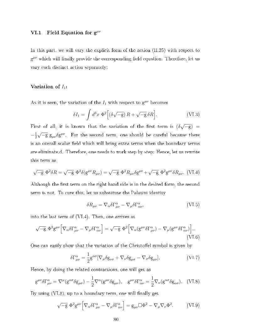
VI.1 Field Equation for gµν
In this part, we will vary the explicit form of the action (II.25) with respect to
gµν which will nally provide the corresponding eld equation. Therefore, let us
vary each distinct action separately:
Variation of I1:
As it is seen, the variation of the I1 with respect to gµν becomes
δI1 =
∫d3x Φ2
[(δ√−g)R +
√−g δR
]. (VI.3)
First of all, it is known that the variation of the rst term is (δ√−g) =
−12
√−g gµνδg
µν . For the second term, one should be careful because there
is an overall scalar eld which will bring extra terms when the boundary terms
are eliminate.d. Therefore, one needs to work step by step: Hence, let us rewrite
this term as
√−g Φ2δR =
√−g Φ2δ(gµνRµν) =
√−g Φ2Rµνδgµν +
√−g Φ2gµνδRµν . (VI.4)
Although the rst term on the right hand side is in the desired form, the second
term is not. To cure this, let us substitute the Palatini identity
δRµν = ∇αδΓαµν −∇µδΓ
ααν , (VI.5)
into the last term of (VI.4). Then, one arrives at
√−g Φ2gµν
[∇αδΓ
αµν −∇µδΓ
ααν
]=√−g Φ2
[∇α(gµνδΓαµν)−∇µ(gµνδΓααν)
]..
(VI.6)
One can easily show that the variation of the Christoel symbol is given by
δΓαµν =1
2gασ[∇µδgνσ +∇νδgµσ −∇σδgµν ], (VI.7)
Hence, by doing the related contractions, one will get as
gµνδΓαµν = ∇µ(gασδgµσ)− 1
2∇α(gµνδgµν), gµνδΓααν =
1
2∇ν(gασδgασ). (VI.8)
By using (VI.8), up to a boundary term, one will nally get
√−g Φ2gµν
[∇αδΓ
αµν −∇µδΓ
ααν
]= gµνΦ2 −∇µ∇νΦ
2. (VI.9)
80
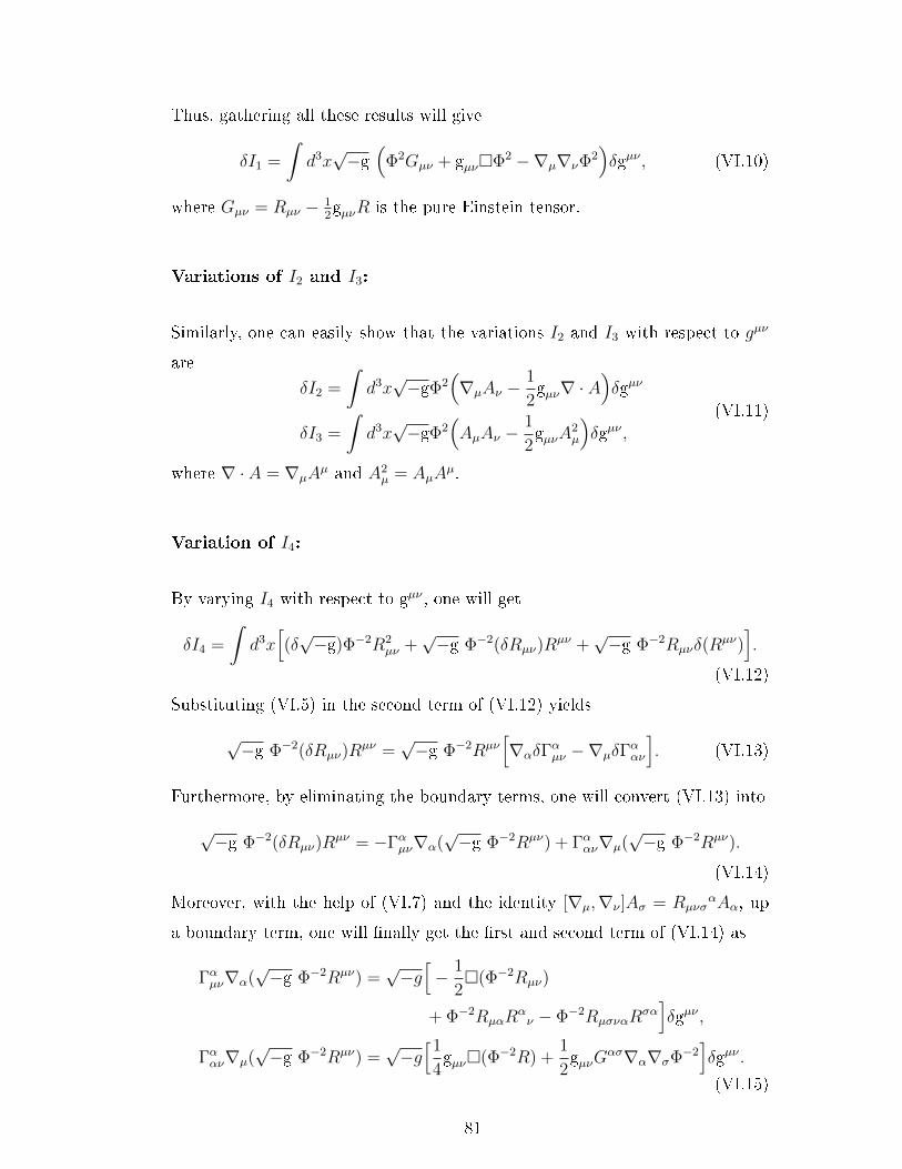
Thus, gathering all these results will give
δI1 =
∫d3x√−g
(Φ2Gµν + gµνΦ2 −∇µ∇νΦ
2)δgµν , (VI.10)
where Gµν = Rµν − 12gµνR is the pure Einstein tensor.
Variations of I2 and I3:
Similarly, one can easily show that the variations I2 and I3 with respect to gµν
are
δI2 =
∫d3x√−gΦ2
(∇µAν −
1
2gµν∇ · A
)δgµν
δI3 =
∫d3x√−gΦ2
(AµAν −
1
2gµνA
2µ
)δgµν ,
(VI.11)
where ∇ · A = ∇µAµ and A2
µ = AµAµ.
Variation of I4:
By varying I4 with respect to gµν , one will get
δI4 =
∫d3x[(δ√−g)Φ−2R2
µν +√−g Φ−2(δRµν)R
µν +√−g Φ−2Rµνδ(R
µν)].
(VI.12)
Substituting (VI.5) in the second term of (VI.12) yields
√−g Φ−2(δRµν)R
µν =√−g Φ−2Rµν
[∇αδΓ
αµν −∇µδΓ
ααν
]. (VI.13)
Furthermore, by eliminating the boundary terms, one will convert (VI.13) into
√−g Φ−2(δRµν)R
µν = −Γαµν∇α(√−g Φ−2Rµν) + Γααν∇µ(
√−g Φ−2Rµν).
(VI.14)
Moreover, with the help of (VI.7) and the identity [∇µ,∇ν ]Aσ = RµνσαAα, up
a boundary term, one will nally get the rst and second term of (VI.14) as
Γαµν∇α(√−g Φ−2Rµν) =
√−g[− 1
2(Φ−2Rµν)
+ Φ−2RµαRαν − Φ−2RµσναR
σα]δgµν ,
Γααν∇µ(√−g Φ−2Rµν) =
√−g[1
4gµν(Φ−2R) +
1
2gµνG
ασ∇α∇σΦ−2]δgµν .
(VI.15)
81

Hence, using this result, (VI.14) becomes
√−g Φ−2(δRµν)R
µν =1
2(Φ−2Gµν) +
1
2gµν(Φ−2R)
+1
2gµνG
ασ∇α∇σΦ−2 − Φ−2RµαRαν + Φ−2RµσναR
σα.
(VI.16)
On the other side, the last term of the (VI.12) can also be written as
√−g Φ−2Rµνδ(R
µν) = 2√−gΦ−2RµαR
ανδgµν +
√−gΦ−2RαβδRαβ. (VI.17)
One should observe that the last term of (VI.17) is nothing but what was found
in (VI.16). Thus, collecting all the tools developed above, one will arrive at
δI4 =
∫d3x√−g
[2Φ−2(Rµσνα −
1
4gµνRαβ)Rαβ
+ (Φ−2Gµν) + gµν(Φ−2R) + gµνGασ∇α∇σΦ−2
].
(VI.18)
Variation of I5:
In this case, the variation of I5 with respect to gµν gives
δI5 =
∫d3x[(δ√−g) Φ−2R2 + 2
√−g Φ−2RδR
]. (VI.19)
Since the last term is not in the desired form, let us rewrite it as
√−g Φ−2RδR =
√−g Φ−2Rδ(gµνRµν)
=√−g Φ−2RRµνδgµν +
√−g Φ−2RgµνδRµν .
(VI.20)
As it was done above, by using (VI.5) and (VI.8), up to a boundary term, one
will get
√−g Φ−2RδR =
√−g[Φ−2RRµν +gµν(Φ−2R)−∇µ∇ν(Φ
−2R)]δgµν . (VI.21)
Hence, plugging (VI.21) into (VI.19) will nally yield
δI5 =
∫d3x√−g[− 1
2gµνΦ
−2R2 + 2Φ−2RRµν
+ 2gµν(Φ−2R)− 2∇µ∇ν(Φ−2R)
]δgµν .
(VI.22)
82

Variation of I6:
To nd the contribution coming from I6, let us vary it with respect to gµν
I6 =
∫d3x
[(δ√−g) Φ−2Rαβ∇αAβ +
√−gΦ−2∇µAν δ(gµαgνβRαβ)
]=
∫d3x√−g[− 1
2gµνδg
µν Φ−2Rαβ∇αAβ + Φ−2Rαν∇µAν δgµα
+ Φ−2Rµβ∇µAν δgνβ + Φ−2∇αAβδRαβ
].
(VI.23)
Using (VI.5) in the last term will turn (VI.23) into
Φ−2∇αAβδRαβ = −δΓσαβ∇σ(Φ−2∇αAβ) + δΓσσβ∇α(Φ−2∇αAβ). (VI.24)
Moreover, by using (VI.7), one will nally get
Φ−2∇αAβδRαβ =[1
2(Φ−2∇µAν) +
1
2gµν∇β∇α(Φ−2∇αAβ)
− 1
2∇α∇ν(Φ
−2∇αAµ)− 1
2∇β∇ν(Φ
−2∇µAβ)]δgµν .
(VI.25)
Thus, with this result, up to a boundary term, one will nally obtain (VI.23) as
I6 =
∫d3x√−g[− 1
2gµν Φ−2Rαβ∇αAβ + Φ−2Rαν∇µA
α
+ Φ−2Rµβ∇βAν +1
2(Φ−2∇µAν)
+1
2gµν∇β∇α(Φ−2∇αAβ)− 1
2∇α∇ν(Φ
−2∇αAµ)
− 1
2∇β∇ν(Φ
−2∇µAβ)]δgµν .
(VI.26)
Variation of I7:
As in the previous cases, by varying I7 with respect to gµν , one will get
δI7 =
∫d3x[(δ√−g) Φ−2RαβAαAβ + 2
√−g Φ−2Rα
νAµAα(δgµν)
+√−g Φ−2AµAνgµαgνβδRαβ
].
(VI.27)
Let us now substitute (VI.5) in the last term of (VI.27)
√−g Φ−2AµAνg
µαgνβδRαβ =√−g Φ−2AµAν∇ζ(gµαgνβδΓ
ζαβ)
−√−g Φ−2AµAν∇α(gµαgνβδΓζζβ).
(VI.28)
83
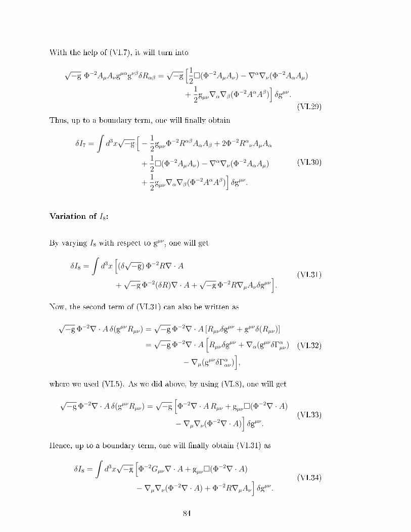
With the help of (VI.7), it will turn into
√−g Φ−2AµAνgµαgνβδRαβ =
√−g[1
2(Φ−2AµAν)−∇α∇ν(Φ
−2AαAµ)
+1
2gµν∇α∇β(Φ−2AαAβ)
]δgµν .
(VI.29)
Thus, up to a boundary term, one will nally obtain
δI7 =
∫d3x√−g[− 1
2gµνΦ
−2RαβAαAβ + 2Φ−2RανAµAα
+1
2(Φ−2AµAν)−∇α∇ν(Φ
−2AαAµ)
+1
2gµν∇α∇β(Φ−2AαAβ)
]δgµν .
(VI.30)
Variation of I8:
By varying I8 with respect to gµν , one will get
δI8 =
∫d3x
[(δ√−g) Φ−2R∇ · A
+√−gΦ−2(δR)∇ · A+
√−gΦ−2R∇µAνδgµν
].
(VI.31)
Now, the second term of (VI.31) can also be written as
√−gΦ−2∇ · Aδ(gµνRµν) =
√−gΦ−2∇ · A [Rµνδgµν + gµνδ(Rµν)]
=√−gΦ−2∇ · A
[Rµνδgµν +∇α(gµνδΓαµν)
−∇µ(gµνδΓααν)],
(VI.32)
where we used (VI.5). As we did above, by using (VI.8), one will get
√−gΦ−2∇ · Aδ(gµνRµν) =
√−g[Φ−2∇ · ARµν + gµν(Φ−2∇ · A)
−∇µ∇ν(Φ−2∇ · A)
]δgµν .
(VI.33)
Hence, up to a boundary term, one will nally obtain (VI.31) as
δI8 =
∫d3x√−g[Φ−2Gµν∇ · A+ gµν(Φ−2∇ · A)
−∇µ∇ν(Φ−2∇ · A) + Φ−2R∇µAν
]δgµν .
(VI.34)
84

Variation of I9:
In this case, the variation of I9 relative to gµν yields
δI9 =
∫d3x[(δ√−g) Φ−2RA2
µ
+√−gΦ−2δ(R)A2
α +√−g Φ−2RAµAνδgµν
].
(VI.35)
Here, the second term of the (VI.35) can be written as
√−gΦ−2A2
βδ(gµνRµν) =
√−gΦ−2A2
β[Rµνδgµν + gµνδRµν ]
=√−gΦ−2A2
β[Rµνδgµν +∇α(gµνδΓαµν)
−∇µ(gµνδΓααν)],
(VI.36)
where we used (VI.5). As we did above, by using (VI.8), up to a boundary term,
one will nally obtain
√−gΦ−2A2
βδ(gµνRµν) =
√−g[Φ−2A2
βRµν + gµν(Φ−2A2β)
−∇µ∇ν(Φ−2A2
β)]δgµν .
(VI.37)
Collecting all these results, one will arrive at
δI9 =
∫d3x√−g[Φ−2A2
βGµν + gµν(Φ−2A2β)
−∇µ∇ν(Φ−2A2
β) + Φ−2RAµAν
]δgµν .
(VI.38)
Variation of I10, I12, I13 and I14:
Finally, by varying I10, I12, I13 and I14 with respect to gµν , one will nally get
δI10 =
∫d3x√−g Φ−2
[− 1
2gµνF
αβFαβ − 2FναFαµ
]δgµν ,
δI12 =
∫d3x√−g[− 1
2gµνΦ
−2AµAν∇µAν
+ Φ−2AνAα∇µAα + Φ−2AµA
α∇αAν
]δgµν ,
δI13 =
∫d3x√−gΦ−2
[− 1
2gµν(∇ · A)2 + 2∇µAν(∇ · A)
]δgµν ,
δI14 =
∫d3x√−g[− 1
2gµν Φ−2A2
αA2β + 2Φ−2AµAνA
2α
]δgµν .
(VI.39)
Gathering all the results developed above, ignoring the boundary terms, one will
thus the full eld equation
85

σΦ2Gµν + σgµνΦ2 − σ∇µ∇νΦ2 − 4σΦ2∇µAν + 2σgµνΦ
2∇ · A− 2σΦ2AµAν + σgµνΦ
2A2 + 2Φ−2[Rµσνα − 14gµνRσα]Rσα + (Φ−2Gµν)
+ 14[gµν−∇µ∇ν ]Φ
−2R + gµνGσα∇σ∇αΦ−2 − 2Gσ
ν∇σ∇µΦ−2
− 2(∇µGσν)(∇σΦ−2) + 3
16gµνΦ
−2R2 − 34Φ−2RRµν + gµνΦ
−2Rαβ∇αAβ
− 2Φ−2Rαν∇µAα − 2Φ−2Rβµ∇βAν −(Φ−2∇µAν)− gµν∇β∇α(Φ−2∇αAβ)
+∇α∇ν(Φ−2∇αAµ) +∇β∇ν(Φ
−2∇µAβ)− gµνΦ
−2RαβAαAβ + 4Φ−2RανAµAα
+ (Φ−2AµAν)− 2∇α∇ν(Φ−2AαAµ) + gµν∇α∇β(Φ−2AαAβ) + Φ−2Gµν∇ · A
+ gµν(Φ−2∇ · A)−∇µ∇ν(Φ−2∇ · A) + Φ−2R∇µAν − 1
2Φ−2GµνA
2
− 12gµν(Φ−2A2) + 1
2∇µ∇ν(Φ
−2A2)− 12Φ−2RAµAν − Φ−2[gµνF
2αβ + 4Fν
αFαµ]
− 12gµνΦ
−2(∇αAβ)2 + Φ−2∇µAα∇νAα + Φ−2∇βAν∇βAµ + gµνΦ
−2AαAβ∇αAβ
− 2Φ−2AνAα∇µAα − 2Φ−2AµA
β∇βAν + 12gµν(∇ · A)2 − 2(∇ · A)∇µAν
− 14gµνΦ
−2A4 + Φ−2AµAνA2 = − 1√
−gδS(Φ)δgµν .
VI.2 Field Equation for Aµ
In this part, by varying the related distinct action that involves gauge eld in
(VI.1) with respect to Aµ, up to a boundary term, one will arrive at
δI2 = −∫d3x√−g (∇µΦ2) δAµ,
δI3 = 2
∫d3x√−gΦ2AµδA
µ,
δI6 = −∫d3x√−g[Rµν∇νΦ−2 +
1
2Φ−2∇µR
]δAµ,
δI7 = 2
∫d3x√−gΦ−2RµνA
ν δAµ,
δI8 = −∫d3x√−g∇µ(Φ−2R) δAµ,
δI9 = 2
∫d3x√−gΦ−2RAµ δA
µ,
δ(I10 + I11) = 4
∫d3x√−g[∇ν(Φ
−2∇µAν)− 3
2∇ν(Φ
−2∇νAµ)]δAµ,
δI12 = −∫d3x√−g[AνAµ∇νΦ
−2 − Φ−2Aν∇µAν + Φ−2Aµ∇νAν]δAµ,
δI13 = −2
∫d3x√−g∇µ(Φ−2∇νA
ν) δAµ,
δI14 = 4
∫d3x√−gΦ−2AµA
2ν δA
µ.
(VI.40)
86
CHAPTER VII
PERTURBATIVE EXPANSION OF THE GENERIC
N-DIMENSIONAL WEYL-INVARIANT HIGHER
CURVATURE GRAVITY THEORIES
In this section, we will study the second-order perturbative expansion of the
generic n-dimensional scale-invariant quadratic curvature gravity theories which
is given by [8]
SWI =
∫dnx√−g
σΦ2R+Φ
2(n−4)n−2
[αR2+βR2
µν+γR2µνρσ
]+SΦ+SAµ , (VII.1)
Needless to say that, since by setting γ = 0 and choose 8α + 3β = 0 in
3-dimensions, (VII.1) will recover the Weyl-gauged New Massive Gravity [8].
Therefore, it is useless to compute its perturbative expansion,separately. Here,
SΦ and SAµ are the generic n-dimensional conformal-invariant obtained in the
second and third chapters. As evaluated in previous chapter, the corresponding
explicit forms of the Weyl-gauged quadratic Ricci scalar is composed of the pure
curvature scalar terms and Abelian gauge elds as
R2 = R2 − 4(n− 1)R(∇ · A)− 2(n− 1)(n− 2)RA2
+ 4(n− 1)2(∇ · A)2 + 4(n− 1)2(n− 2)A2(∇ · A)
+ (n− 1)2(n− 2)2A4,
(VII.2)
87
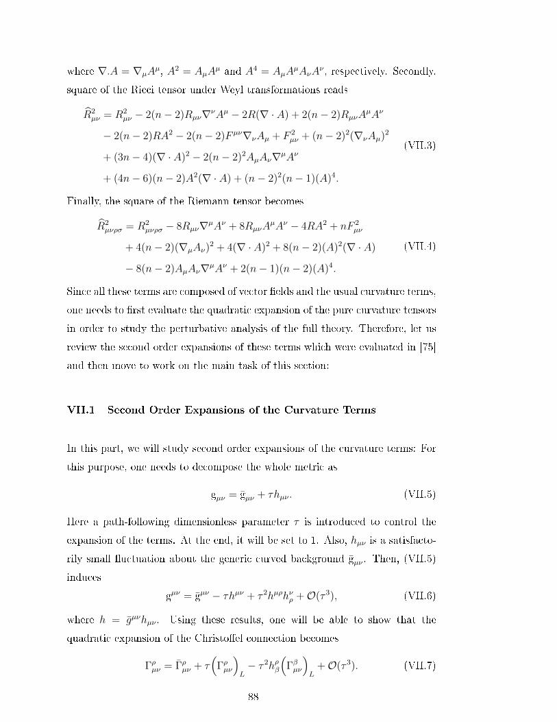
where ∇.A = ∇µAµ, A2 = AµA
µ and A4 = AµAµAνA
ν , respectively. Secondly,
square of the Ricci tensor under Weyl transformations reads
R2µν = R2
µν − 2(n− 2)Rµν∇νAµ − 2R(∇ · A) + 2(n− 2)RµνAµAν
− 2(n− 2)RA2 − 2(n− 2)F µν∇νAµ + F 2µν + (n− 2)2(∇νAµ)2
+ (3n− 4)(∇ · A)2 − 2(n− 2)2AµAν∇µAν
+ (4n− 6)(n− 2)A2(∇ · A) + (n− 2)2(n− 1)(A)4.
(VII.3)
Finally, the square of the Riemann tensor becomes
R2µνρσ = R2
µνρσ − 8Rµν∇µAν + 8RµνAµAν − 4RA2 + nF 2
µν
+ 4(n− 2)(∇µAν)2 + 4(∇ · A)2 + 8(n− 2)(A)2(∇ · A)
− 8(n− 2)AµAν∇µAν + 2(n− 1)(n− 2)(A)4.
(VII.4)
Since all these terms are composed of vector elds and the usual curvature terms,
one needs to rst evaluate the quadratic expansion of the pure curvature tensors
in order to study the perturbative analysis of the full theory. Therefore, let us
review the second order expansions of these terms which were evaluated in [75]
and then move to work on the main task of this section:
VII.1 Second Order Expansions of the Curvature Terms
In this part, we will study second order expansions of the curvature terms: For
this purpose, one needs to decompose the whole metric as
gµν = gµν + τhµν . (VII.5)
Here a path-following dimensionless parameter τ is introduced to control the
expansion of the terms. At the end, it will be set to 1. Also, hµν is a satisfacto-
rily small uctuation about the generic curved background gµν . Then, (VII.5)
induces
gµν = gµν − τhµν + τ 2hµρhνρ +O(τ 3), (VII.6)
where h = gµνhµν . Using these results, one will be able to show that the
quadratic expansion of the Christoel connection becomes
Γρµν = Γρµν + τ(
Γρµν
)L− τ 2hρβ
(Γβµν
)L
+O(τ 3). (VII.7)
88
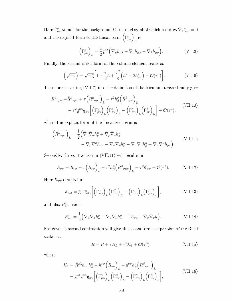
Here Γρµν stands for the background Christoel symbol which requires ∇ρgµν = 0
and the explicit form of the linear term(
Γρµν
)Lis
(Γρµν
)L
=1
2gρλ(∇µhνλ + ∇νhµλ − ∇λhµν
). (VII.8)
Finally, the second-order form of the volume element reads as(√−g)
=√−g[1 +
τ
2h+
τ 2
8
(h2 − 2h2
µν
)+O(τ 3)
]. (VII.9)
Therefore, inserting (VII.7) into the denition of the Riemann tensor nally give
Rµνρσ =Rµ
νρσ + τ(Rµ
νρσ
)L− τ 2hµβ
(Rβ
νρσ
)L
− τ 2gµαgβγ
[(Γγρα
)L
(Γβσν
)L−(
Γγσα
)L
(Γβρν
)L
]+O(τ 3),
(VII.10)
where the explicit form of the linearized term is(Rµ
νρσ
)L
=1
2
(∇ρ∇σh
µν + ∇ρ∇νh
µσ
− ∇ρ∇µhσν − ∇σ∇ρhµν − ∇σ∇νh
µρ + ∇σ∇µhρν
).
(VII.11)
Secondly, the contraction in (VII.11) will results in
Rνσ = Rνσ + τ(Rνσ
)L− τ 2hµβ
(Rβ
νµσ
)L− τ 2Kνσ +O(τ 3). (VII.12)
Here Kνσ stands for
Kνσ = gµαgβγ
[(Γγµα
)L
(Γβσν
)L−(
Γγσα
)L
(Γβµν
)L
], (VII.13)
and also RLνσ reads
RLνσ =
1
2
(∇µ∇σh
µν + ∇µ∇νh
µσ − hσν − ∇σ∇νh
). (VII.14)
Moreover, a second contraction will give the second-order expansion of the Ricci
scalar as
R = R + τRL + τ 2K1 +O(τ 3), (VII.15)
where
K1 = Rρλhαρhαλ − hνσ
(Rνσ
)L− gνσhµβ
(Rβ
νµσ
)L
− gνσgµαgβγ
[(Γγµα
)L
(Γβσν
)L−(
Γγσα
)L
(Γβµν
)L
],
(VII.16)
89

and
RL = gαβRLαβ − Rαβhαβ. (VII.17)
Thus, collecting all these results, one will nally obtain linearized Einstein tensor
as
GLµν = (Rµν)L − 1
2gµνR
L − 2Λ
n− 2hµν . (VII.18)
VII.2 Second Order Expansion of the Action
In this part, we will nd the quadratic expansion of the (VII.1) in generic n-
dimensional (A)dS backgrounds whose curvature terms are
Rµρνσ =2Λ
(n− 1)(n− 2)(gµν gρσ − gµσgνρ), Rµν =
2Λ
n− 2gµν , R =
2nΛ
n− 2,
(VII.19)
and in which the classical solutions are
Φvac = m(n−2)/2, Aµvac = 0, gµν = gµν . (VII.20)
From now, let us study the quadratic expansion of the full theory by working
on each term, separately:
Quadratic Expansion of the α-Part
Throughout the calculations, we will need the quadratic uctuation of the elds.
Therefore, by using the Binomial expression of
(1 + x)p = 1 + px+p(p− 1)
2!x2 + . . . , (VII.21)
one will obtain the scalar part up to quadratic order as
(Φ2(n−4)n−2 )2nd = m
n−4n−2
[1 + τ C(τ)
ΦL
√m
+ τ 2 C(τ2)
Φ2L
m
]+O(τ 3), (VII.22)
where
C(τ) =2(n− 4)
n− 2, C(τ2) =
(n− 4)(n− 6)
(n− 2)2. (VII.23)
Let us now rst nd the quadratic uctuations come from the α-part:
90

For R2-term:
By using above mentioned identity, one will obtain the quadratic expression of
the term as
(√−gΦ
2(n−4)n−2 R2
)2nd
=√−g m
n−4n−2
R2 + τ
[2RRL +
C(τ)R2
√m
ΦL +R2
2h
]+ τ 2
[2RK1 +R2
L +2C(τ)R√
mΦLRL
+C(τ2)R
2
mΦ2L + RhRL +
C(τ)R2
2√mhΦL
+R2
8h2 − R2
4h2µν
].
(VII.24)
Before going further, one needs to rst nd the explicit form of the K1: Using
the explicit form of the linearized form of the curvature tensors and (VII.19) as
well as the identity [∇µ,∇ν ]Mρ = RµνραMα will yield
K1 = −1
2hµνRL
µν −1
4hRL +
2Λ
n− 2h2µν −
Λ
2(n− 2)h2. (VII.25)
Thus, by substituting (VII.25) and (VII.19) in (VII.24), one will nally obtain
the quadratic expansion of the term in n-dimensional (A)dS background as
(√−gΦ
2(n−4)n−2 R2
)2nd
=√−gm
n−4n−2
4n2Λ2
(n− 2)2+ τ
[ 4nΛ
n− 2RL +
4n2C(τ)Λ2
√m(n− 2)2
ΦL +2n2Λ2
(n− 2)2h]
+ τ 2[R2L −
2nΛ
n− 2hµνRL
µν +nΛ
n− 2hRL
− n(n− 8)Λ2
(n− 2)2h2µν +
n(n− 4)Λ2
2(n− 2)2h2
+4nC(τ)Λ√m(n− 2)
ΦLRL +4n2C(τ2)Λ
2
m(n− 2)2Φ2L
+2n2C(τ)Λ
2
√m(n− 2)2
hΦL].
(VII.26)
91
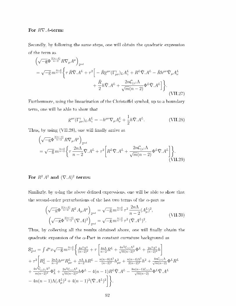
For R∇.A-term:
Secondly, by following the same steps, one will obtain the quadratic expression
of the term as(√−gΦ
2(n−4)n−2 R∇µA
µ)
2nd
=√−gm
n−4n−2
τ R∇.AL + τ 2
[− Rgµν(Γγµν)LALγ +RL∇.AL − Rhµν∇µA
Lν
+R
2h∇.AL +
2nC(τ )Λ√m(n− 2)
ΦL∇.AL].
(VII.27)
Furthermore, using the linearization of the Christoel symbol, up to a boundary
term, one will be able to show that
gµν(Γγµν)LALγ = −hµν∇µA
Lν +
1
2h∇.AL. (VII.28)
Thus, by using (VII.28), one will nally arrive at(√−gΦ
2(n−4)n−2 R∇µA
µ)
2nd
=√−gm
n−4n−2
τ
2nΛ
n− 2∇.AL + τ 2
[RL∇.AL +
2nC(τ )Λ√m(n− 2)
ΦL∇.AL]
.
(VII.29)
For R2A2 and (∇.A)2 terms:
Similarly, by using the above dened expressions, one will be able to show that
the second-order perturbations of the last two terms of the α-part as(√−gΦ
2(n−4)n−2 R2AµA
µ)
2nd=√−gm
n−4n−2 τ 2 2nΛ
n− 2(ALµ)2,(√
−gΦ2(n−4)n−2 (∇.A)2
)2nd
=√−gm
n−4n−2 τ 2 (∇.AL)2.
(VII.30)
Thus, by collecting all the results obtained above, one will nally obtain the
quadratic expansion of the α-Part in constant curvature background as
Sα2nd
=∫dnx√−gm
n−4n−2
4n2Λ2
(n−2)2 + τ
[4nΛn−2
RL +4n2C(τ)Λ
2
√m(n−2)2 ΦL + 2n2Λ2
(n−2)2h
]+ τ 2
[R2L − 2nΛ
n−2hµνRL
µν + nΛn−2
hRL − n(n−8)Λ2
(n−2)2 h2µν + n(n−4)Λ2
2(n−2)2 h2 +
4nC(τ)Λ√m(n−2)
ΦLRL
+4n2C(τ2)Λ
2
m(n−2)2 Φ2L +
2n2C(τ)Λ2
√m(n−2)2hΦL − 4(n− 1)RL∇.AL − 8n(n−1)C(τ)Λ√
m(n−2)ΦL∇.AL
− 4n(n− 1)Λ(ALµ)2 + 4(n− 1)2(∇.AL)2
].
92

Quadratic Expansion of the β-Part
In this part, we will study second-order perturbative expansion of the β part of
the whole action:
For R2µν:
By using above mentioned identity, one will obtain the quadratic expression of
the following term as(√−gΦ
2(n−4)n−2 R2
µν
)2nd
=√−gm
n−4n−2
R2µν + τ
[R2µν
2h+ 2RµνRL
µν − 2RµαRσαh
µσ +C(τ)R
2µν√
mΦL]
+ τ 2[(RL
µν)2 − 2Rµνhθκ(R
κµθν)L − 2RµνKµν
− 4RLµνR
µαh
να + 2RµνRµαh
νζhαζ + RµνRσαhµσhνα
+ hRLµνR
µν − hRµαRσαh
µσ +R2µν
8h2 −
R2µν
4h2αβ
+C(τ)R
2µν
2√m
hΦL +2C(τ)R
µν
√m
ΦLRLµν
−2C(τ)Rµ
αRσα√m
hµσΦL +C(τ2)R
2µν
mΦ2L
].
(VII.31)
To nd the explicit result, one must rst nd what the following terms acquire.
First of all, as we did above, by using the linearized Riemann tensor, in (A)dS
backgrounds, one will obtain
gµνhθκ(Rκµθν)L = hµνRL
µν −2nΛ
(n− 1)(n− 2)h2µν +
2Λ
(n− 1)(n− 2)h2. (VII.32)
Secondly,
gµνRLµν = RL +
2Λ
n− 2h, (VII.33)
and nally
gµνKµν = −3
2hµνRL
µν+1
4hRL+
2nΛ
(n− 1)(n− 2)h2µν+
(n− 5)Λ
2(n− 1)(n− 2)h2. (VII.34)
93

Thus, by gathering all these results, one will nd the quadratic expansion of the
term in (A)dS background as(√−gΦ
2(n−4)n−2 R2
µν
)2nd
=√−gm
n−4n−2
4nΛ2
(n− 2)2+ τ
[ 4Λ
n− 2RL +
2nΛ2
(n− 2)2h+
4nC(τ)Λ2
√m(n− 2)2
ΦL]
+ τ 2[(RL
µν)2 − 6Λ
n− 2hµνRL
µν +Λ
n− 2hRL
+(12− n)Λ2
(n− 2)2h2µν +
(n− 4)Λ2
2(n− 2)2h2
+2nC(τ)Λ
2
√m(n− 2)2
hΦL +4C(τ)Λ√m(n− 2)
ΦLRL
+4nC(τ2)Λ
2
m(n− 2)2Φ2L
].
(VII.35)
For Rµν∇µAν, RµνAµA
µ, F 2µν, F
µν∇νAµ and (∇νAµ)2 terms:
Since it is straight forward, by suppressing the intermediate steps, one will nally
obtain the quadratic expansion of the remaining terms as(√−gΦ
2(n−4)n−2 Rµν∇µAν
)2nd
=√−gm
n−4n−2
τ
2Λ
n− 2∇ · AL
+ τ 2[RLµν∇µAνL −
2Λ
n− 2hµν∇µA
Lν +
2C(τ)Λ√m(n− 2)
ΦL∇ · AL],
(VII.36)
and (√−gΦ
2(n−4)n−2 RµνAµA
µ)
2nd=√−g m
n−4n−2 τ 2 2Λ
n− 2(ALµ)2,(√
−gΦ2(n−4)n−2 F 2
µν
)2nd
=√−g m
n−4n−2 τ 2 (FL
µν)2,(√
−gΦ2(n−4)n−2 F µν∇νAµ
)2nd
=√−g m
n−4n−2 τ 2 F µν
L ∇νALµ ,(√
−gΦ2(n−4)n−2 (∇νAµ)2
)2nd
=√−g m
n−4n−2 τ 2 (∇νA
Lµ)2.
(VII.37)
Thus, by collecting all the results obtained above, up to a boundary term, one
will nally obtain the quadratic expansion of the β-Part in constant curvature
94

background as
Sβ2nd
=
∫dnx√−gm
n−4n−2
4nΛ2
(n− 2)2+ τ
[ 4Λ
n− 2RL +
2nΛ2
(n− 2)2h+
4nC(τ)Λ2
√m(n− 2)2
ΦL]
+ τ 2[(RL
µν)2 − 6Λ
n− 2hµνRL
µν +Λ
n− 2hRL +
(12− n)Λ2
(n− 2)2h2µν
+(n− 4)Λ2
2(n− 2)2h2 +
2nC(τ)Λ2
√m(n− 2)2
hΦL +4C(τ)Λ√m(n− 2)
ΦLRL +4nC(τ2)Λ
2
m(n− 2)2Φ2L
− nRL∇ · AL + 4Λhµν∇µALν −
8(n− 1)C(τ)Λ√m(n− 2)
ΦL∇ · AL
− 4(n− 1)Λ(ALµ)2 + (FLµν)
2 − 2(n− 2)F µνL ∇νA
Lµ
+ (n− 2)2(∇νALµ)2 + (3n− 4)(∇ · AL)2
].
(VII.38)
Quadratic Expansion of the γ-Part
For R2µνρσ:
Let us now nd the quadratic expansion of the R2µνρσ. As we did before, one
will obtain(√−gΦ
2(n−4)n−2 R2
µνρσ
)2nd
=(√−gΦ
2(n−4)n−2 gµζg
νλgρβgσκRζνρσR
µλβκ
)2nd
=√−gm
n−4n−2
Rµ
λβκRµλβκ + τ
[2Rµ
λβκ(Rµλβκ)L − 2Rµ
λβσR
µλβκh
σκ
− RµνβκRµ
λβκhνλ + RζλβκRµ
λβκhµζ + RµλβκRµ
λβκ
( C(τ)√m
ΦL +1
2h)]
+ τ 2
[− 2Rµ
λβκKµλβκ + gµζ gνλgρβ gσκ(Rζ
νρσ)L(Rµλβκ)L − 4Rµ
λβσ(Rµ
λβκ)Lhσκ
− 2Rµνβκ(Rµ
λβκ)Lhνλ + 3Rµ
λβσR
µλβκh
σαhκα + RµλρσR
µλβκh
ρβhσκ
+2C(τ)Rµ
λβκ
√m
ΦL(Rµλβκ)L −
2C(τ)RµλβσR
µλβκ√
mΦLhσκ +
C(τ2)RµλβκRµ
λβκ
mΦ2L
+ Rµλβκh(Rµ
λβκ)L − RµλβσR
µλβκhh
σκ +C(τ)Rµ
λβκRµλβκ
2√m
hΦL
+Rµ
λβκRµλβκ
8h2 − Rµ
λβκRµλβκ
4h2µν
].
(VII.39)
95
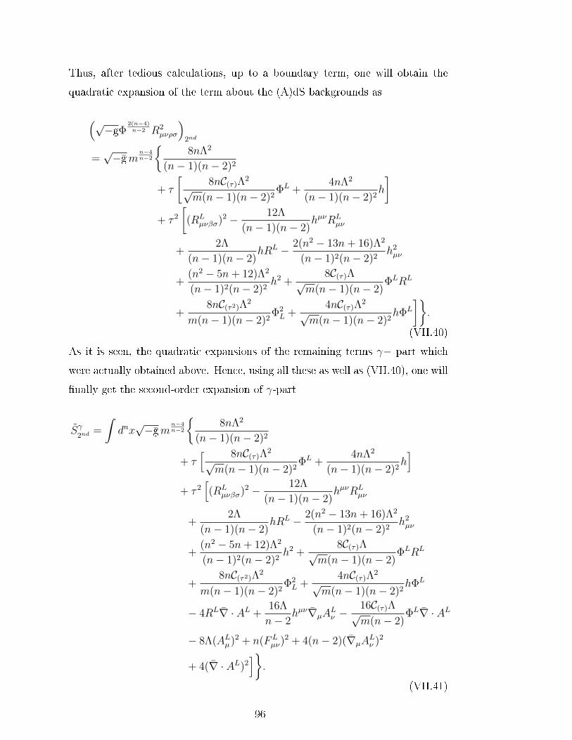
Thus, after tedious calculations, up to a boundary term, one will obtain the
quadratic expansion of the term about the (A)dS backgrounds as
(√−gΦ
2(n−4)n−2 R2
µνρσ
)2nd
=√−gm
n−4n−2
8nΛ2
(n− 1)(n− 2)2
+ τ
[8nC(τ)Λ
2
√m(n− 1)(n− 2)2
ΦL +4nΛ2
(n− 1)(n− 2)2h
]+ τ 2
[(RL
µνβσ)2 − 12Λ
(n− 1)(n− 2)hµνRL
µν
+2Λ
(n− 1)(n− 2)hRL − 2(n2 − 13n+ 16)Λ2
(n− 1)2(n− 2)2h2µν
+(n2 − 5n+ 12)Λ2
(n− 1)2(n− 2)2h2 +
8C(τ)Λ√m(n− 1)(n− 2)
ΦLRL
+8nC(τ2)Λ
2
m(n− 1)(n− 2)2Φ2L +
4nC(τ)Λ2
√m(n− 1)(n− 2)2
hΦL
].
(VII.40)
As it is seen, the quadratic expansions of the remaining terms γ− part which
were actually obtained above. Hence, using all these as well as (VII.40), one will
nally get the second-order expansion of γ-part
Sγ2nd
=
∫dnx√−gm
n−4n−2
8nΛ2
(n− 1)(n− 2)2
+ τ[ 8nC(τ)Λ
2
√m(n− 1)(n− 2)2
ΦL +4nΛ2
(n− 1)(n− 2)2h]
+ τ 2[(RL
µνβσ)2 − 12Λ
(n− 1)(n− 2)hµνRL
µν
+2Λ
(n− 1)(n− 2)hRL − 2(n2 − 13n+ 16)Λ2
(n− 1)2(n− 2)2h2µν
+(n2 − 5n+ 12)Λ2
(n− 1)2(n− 2)2h2 +
8C(τ)Λ√m(n− 1)(n− 2)
ΦLRL
+8nC(τ2)Λ
2
m(n− 1)(n− 2)2Φ2L +
4nC(τ)Λ2
√m(n− 1)(n− 2)2
hΦL
− 4RL∇ · AL +16Λ
n− 2hµν∇µA
Lν −
16C(τ)Λ√m(n− 2)
ΦL∇ · AL
− 8Λ(ALµ)2 + n(FLµν)
2 + 4(n− 2)(∇µALν )2
+ 4(∇ · AL)2].
(VII.41)
96

Quadratic Expansion of the Weyl-invariant Scalar Field Part
The action for the generic n-dimensional Weyl-invariant scalar eld is given by
[8]
SΦ = −1
2
∫dnx√−g (DµΦDµ + νΦ
2nn−2 Φ). (VII.42)
By following using the quadratic expansion of the terms, up to a boundary term,
one will nally obtain the second order expansion of SΦ
(SΦ)(2nd) =
∫ √−gm
n−4n−2
− νm
4n−2
2
+ τ[− νm
4n−2
4h−
νm−(n−10)2(n−2) B(τ)
2ΦL]
+ τ 2[− m
−(n−4)(n−2)
2(∂µΦL)2 +
(n− 2)m−(n−6)2(n−2)
2ALµ∂
µΦL
− (n− 2)2m2
n−2
8(ALµ)2 −
νm−(n−6)(n−2) B(τ2)
2Φ2L
−νm
−(n−10)2(n−2) B(τ)
4hΦL − νm
4n−2
16h2 +
νm4
n−2
8h2µν
],
(VII.43)
where
B(τ) =2n
n− 2, B(τ2) =
n(n+ 2)
(n− 2)2. (VII.44)
Thus, by collecting all the results obtained above, one will nally obtain L(τ 1)
part as
L(τ 1) =( n
n− 2m
n−62 ΦL +
1
4mn−4h
)(CΛ2 + 4σΛm2 − νm4
), (VII.45)
where
C ≡ 8(n− 4)
(n− 2)2
(nα + β +
2γ
n− 1
). (VII.46)
97

On the other hand L(τ 2)-part as
L(τ 2) = −1
2mn−4hµν
( 4n
n− 2α +
4
n− 1β − 8
n− 1γ)
ΛGLµν
+ (2α + β + 2γ)(gµν− ∇µ∇ν
)RL
+2Λ
n− 2
(2α +
β
n− 1− 2(n− 3)
n− 1γ)gµνRL
+ (β + 4γ)GLµν + σm2GLµν
+mn−2
2
C Λ
m2+ 2σ
RLΦL −
1
2(∂µΦL)2
+n
2(n− 2)
n(n− 6)C
(n− 2)
Λ2
m2+ 4σΛ− (n+ 2)
n− 2m2ν
Φ2L
−mn−4
4(n− 1)α + nβ + 4γ
RL∇ · AL
−mn−2
2
2(n− 1)C Λ
m2+ 4σ(n− 1) +
n− 2
2
ΦL∇ · AL
+mn−4
4(n− 1)2α + nβ + 4γ
(∇ · AL)2
+1
2mn−4
(n2 − 2n+ 2)β + 2(3n− 4)γ + 2ε
(FL
µν)2
− 2mn−2
(2n(n− 1)α + (3n− 4)β + 8γ
) Λ
m2
+(n− 1)(n− 2)
2σ +
(n− 2)2
16
A2L.
(VII.47)
Alternatively, one can also evaluate the second order expansion of the quadratic
curvature parts by mean of the results obtained in [19]: That is, writing∫dnx√−gΦ
2(n−4)n−2
(αR2 + βR2
µν + γR2µνρσ
)=
∫dnx√−g(
mn−2
2 + τΦL
) 2(n−4)n−2
(X + τX(1) + τ 2X(2)
),
(VII.48)
will yield
X ≡ nC2(n− 4)
Λ2, X(1) ≡ nC4(n− 4)
Λ2h+(n− 2)C2(n− 4)
ΛRL. (VII.49)
To get the quadratic part X(2), let us modify it in the form:
X(2) =[√−g(αR2 + βR2
µν + γR2µνρσ
)](2)
=[√−g(
(α− γ)R2 + (β + 4γ)R2µν + γχE
)](2)
,
(VII.50)
98
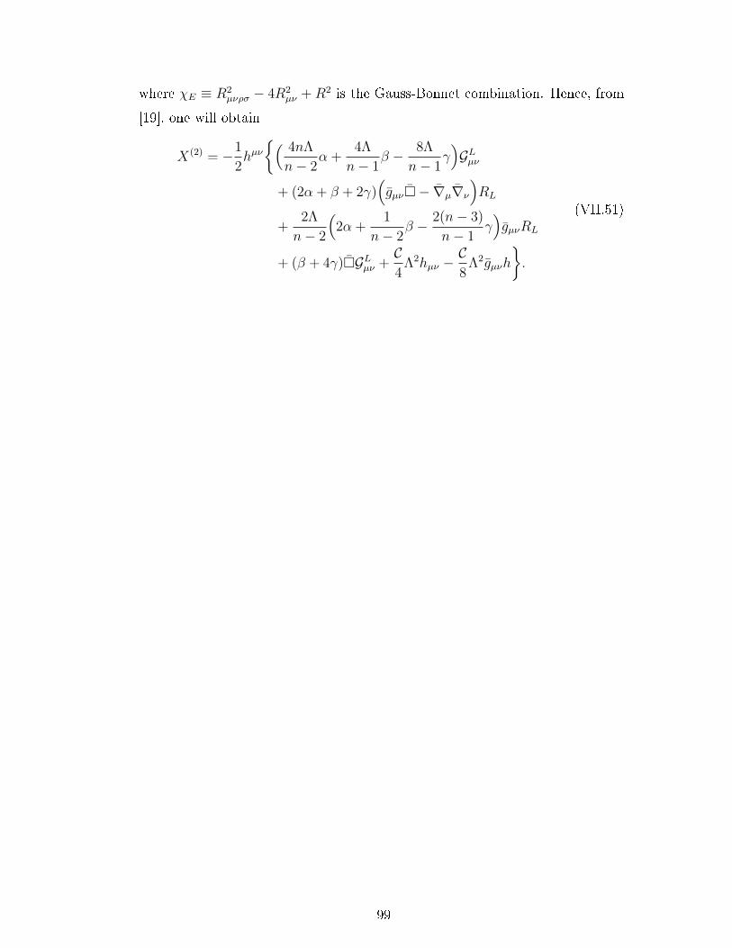
where χE ≡ R2µνρσ − 4R2
µν + R2 is the Gauss-Bonnet combination. Hence, from
[19], one will obtain
X(2) = −1
2hµν( 4nΛ
n− 2α +
4Λ
n− 1β − 8Λ
n− 1γ)GLµν
+ (2α + β + 2γ)(gµν− ∇µ∇ν
)RL
+2Λ
n− 2
(2α +
1
n− 2β − 2(n− 3)
n− 1γ)gµνRL
+ (β + 4γ)GLµν +C4
Λ2hµν −C8
Λ2gµνh
.
(VII.51)
99

100

CURRICULUM VITAE
PERSONAL INFORMATION
Surname, Name: Dengiz, Suat
Nationality: Turkish (TC)
Date and Place of Birth: 01 February 1984, Diyarbakr/Turkey
Marital Status: Single
Phone: +90 (312) 210 5068 (oce)
EDUCATION
Degree Institution Year of Graduation
Ph.D. Physics, Middle East Technical University 2014
M.S. Physics, Middle East Technical University 2011
B.S. Physics Engineering, Hacettepe University 2008
PROFESSIONAL EXPERIENCE
Year Place Enrollment
2013-2014 METU TUBTAK Project Assistant (113F155)
2011-2013 METU TUBTAK Project Assistant (109T748)
2011-2013 METU Teaching Assistant, Mathematical Physics
2009-2011 METU Teaching Assistant, Physics Laboratories
101
RESEARCH INTERESTS
• Classical and Quantum Gravity, Quantum Field Theories, Cosmology and
Black Holes
PUBLICATIONS AND PREPRINTS
• Weyl-invariant SU(N) Einstein-Yang-Mills theory and spontaneous gen-
eration of vacuum expectation value for Higgs-type eld, arXiv:1404.2714,
(2014). Suat Dengiz.
• Scattering in Topologically Massive Gravity, Chiral Gravity and the cor-
responding Anyon-Anyon Potential Energy. Phys. Rev. D 89, 024033
(2014). Suat Dengiz, Ercan Klçarslan and Bayram Tekin.
• Weyl-gauging of Topologically Massive Gravity. Phys. Rev. D 86,
104014 (2012). Suat Dengiz, Ercan Klçarslan and Bayram Tekin.
• Weyl-Invariant Higher Curvature Gravity Theories in n Dimensions.
Phys. Rev. D 85, 064016 (2012). M. Reza Tanhayi, Suat Dengiz and
Bayram Tekin.
• Unitarity of Weyl-Invariant New Massive Gravity and Generation of Gravi-
ton Mass via Symmetry Breaking. Phys. Rev. D 85, 064008 (2012). M.
Reza Tanhayi, Suat Dengiz and Bayram Tekin.
• Higgs Mechanism for New Massive Gravity and Weyl-Invariant Exten-
sions of Higher Derivative Theories. Phys. Rev. D 84, 024033 (2011).
Suat Dengiz and Bayram Tekin.
CONFERENCES, WORKSHOPS, SCHOOLS ANDMEETINGS AT-
TENDED
• 13th Workshop on Dualities and Integrable Systems, Koç University, s-
tanbul 19-20 April, 2014, Turkey,
102
• Lectures on Functional Renormalization and Asymptotic Safety by Roberto
Percacci, METU, Ankara 13-14 February 2013, Turkey,
• 11th Workshop on Dualities and Integrable Systems, Pamukkale Univer-
sity, Denizli 21-23 April 2012, Turkey, Given Talk: Higgs-type mecha-
nism for graviton,
• High Energy Physics Days (YEF gunleri), Ankara University, Ankara
27-30 December 2011, Turkey, Given Talk: Higgs Mechanism for New
Massive Gravity and Weyl-invariant Extensions of Higher Derivative The-
ories,
• Lectures on Up from String Theory: The mathematics of branes in String
and M-theory by Neil Lambert, METU, Ankara Fall 2011, Turkey,
• Recent Advances in Quantum Field and String Theories, Free University,
Tbilisi 26-30 September 2011, Georgia, Given Talk: Higgs Mechanism
for New Massive Gravity and Weyl-invariant Extensions of Higher Deriva-
tive Theories,
• Strings, Branes and Supergravity, Koç University, stanbul August 1-5
2011, Turkey,
• 9th Workshop on Dualities and Integrable Systems, Yeditepe University,
Istanbul 23-25 April 2010, Turkey.
COMPUTER SKILLS
• LATEX, Mathematica, MS Oce, MS Windows.
103


