Page 1
What can we learn/predict from global MHD models?
Seth G. Claudepierre, The Aerospace Corporation
Contributors: Mary Hudson, Bill Lotko, Scot Elkington, Mike Wiltberger, Richard Denton, John Lyon, Frank Toffoletto, Asher Pembroke, Kazue Takahashi
Page 2
What can we learn from global MHD models?
“The source of the oscillations driving field line resonances(FLRs) in the magnetosphere remains controversial.” – Stephenson and Walker, AG, [2010].
Individual solar wind parameters can be isolated in global MHD simulations to asses their role in the generation of magnetospheric ULF waves (externally driven, Pc4-5 waves).
Page 3
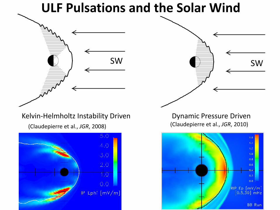
Kelvin-Helmholtz Instability Driven Dynamic Pressure Driven
SW SW
→ Numerical experiments with a global MHD simulation
(Claudepierre et al., JGR, 2008) (Claudepierre et al., JGR, 2010)
ULF Pulsations and the Solar Wind
Page 4
Kelvin-Helmholtz Instability Driven Dynamic Pressure Driven
SW SW
(Claudepierre et al., JGR, 2008) (Claudepierre et al., JGR, 2010)
ULF Pulsations and the Solar Wind
Page 5
Dynamic Pressure Simulations
SW
• Four LFM simulations: (3) monochromatic ULF frequencies (10, 15, 25 mHz): (1) continuum of ULF frequencies (0-30 mHz): • All other input parameters the same: n0 = 5 particles/cm3 B = (0, 0, +5) nT Vx = 600 km/s Vy = Vz = 0 km/s Cs out of phase (→ Pth ~ nCs
2 = const )
)sin()( 0 tCntn ω+=
∑ ++=j
jjtDntn )sin()( 0 ξω
Solar Wind Driving
)~( 2vnpdyn
Page 6
Monochromatic and Continuum Simulation
∑ ++=j
jjtDntn )sin()( 0 ξω
Solar Wind Driving
)sin()( 0 tCntn ω+=
)~( 2vnpdyn
Page 7
10 mHz Simulation EL Wave Power, Equatorial Plane
2/1
),()(
)],([FFT),(
=
=
∫b
a
f
f
L
dffxPxRIP
txEfxP
[fa, fb] = [9.5,10.5] mHz
*Claudepierre et al., JGR, 2010
Xgsm
Ygsm RIP EL [mV/m]
Page 8
10 mHz Simulation EL Wave Power, 15 MLT Meridional Plane
*Claudepierre et al., JGR, 2010 Rgsm
Zgsm
15 MLT
2/1
),()(
)],([FFT),(
=
=
∫b
a
f
f
L
dffxPxRIP
txEfxP
[fa, fb] = [9.5,10.5] mHz RIP EL [mV/m]
Page 9
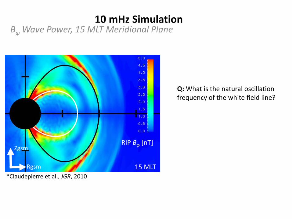
10 mHz Simulation Bφ Wave Power, 15 MLT Meridional Plane
*Claudepierre et al., JGR, 2010
2/1
),()(
)],([FFT),(
=
=
∫b
a
f
fdffxPxRIP
txBfxP
ϕ
[fa, fb] = [9.5,10.5] mHz
Rgsm
Zgsm
15 MLT
RIP Bφ [nT]
Page 10
10 mHz Simulation Bφ Wave Power, 15 MLT Meridional Plane
*Claudepierre et al., JGR, 2010 Rgsm
Zgsm
15 MLT
RIP Bφ [nT]
Q: What is the natural oscillation frequency of the white field line?
Page 11
10 mHz Simulation Bφ Wave Power, 15 MLT Meridional Plane
*Claudepierre et al., JGR, 2010 Rgsm
Zgsm
15 MLT
RIP Bφ [nT]
Q: What is the natural oscillation frequency of the white field line? A: 1
)(2
−
= ∫
N
SA
n sVdsnf (WKB)
Page 12
10 mHz Simulation Bφ Wave Power, 15 MLT Meridional Plane
*Claudepierre et al., JGR, 2010 Rgsm
Zgsm
15 MLT
RIP Bφ [nT]
Q: What is the natural oscillation frequency of the white field line? A:
mHz 10)(
2
1
1
≈
=
−
∫f
sVdsnf
N
SA
n (WKB)
Page 13
10 mHz Simulation EL, Spectral Density, 15 MLT Meridian
*Claudepierre et al., JGR, 2010
1
)(2
−
= ∫
N
S An sV
dsnf (WKB)
RIP EL [mV/m]
RIP EL [mV/m]
XY-plane
15 MLT-plane
Page 14
10 mHz Simulation EL, Bφ Field-Aligned Mode Structure
*Claudepierre et al., JGR, 2010
RIP EL [mV/m]
RIP Bφ [nT]
15 MLT-plane
15 MLT-plane
Page 15
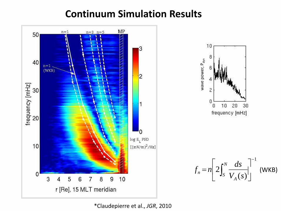
Continuum Simulation Results
*Claudepierre et al., JGR, 2010 w
ave
pow
er, P
dyn
1
)(2
−
= ∫
N
SA
n sVdsnf (WKB)
Page 16
LFM (no plasmasphere) MP
Claudepierre et al., JGR, 2010 Er wave power 15 MLT
Page 17
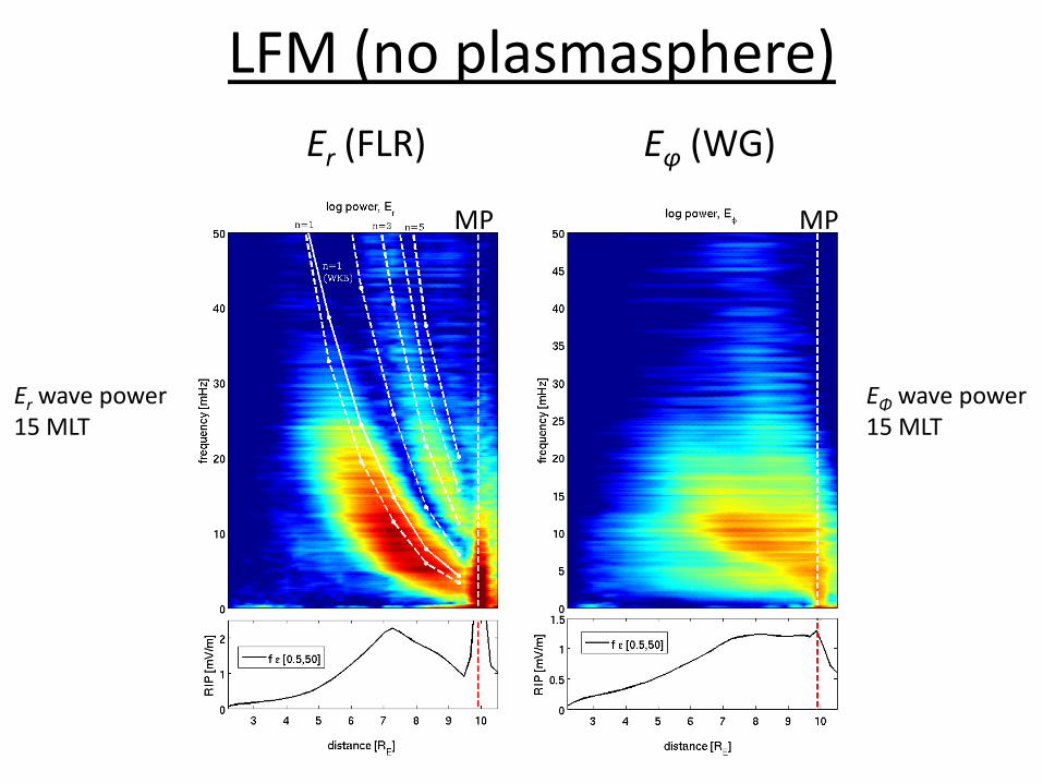
LFM (no plasmasphere) Er (FLR) Eφ (WG)
MP MP
Er wave power 15 MLT
EΦ wave power 15 MLT
Page 18
LFM (no plasmasphere) Er (FLR) Eφ (WG) Bz (WG)
MP MP MP
Page 19
LFM
(no
plas
mas
pher
e)
LFM
-RCM
(w/ p
lasm
asph
ere)
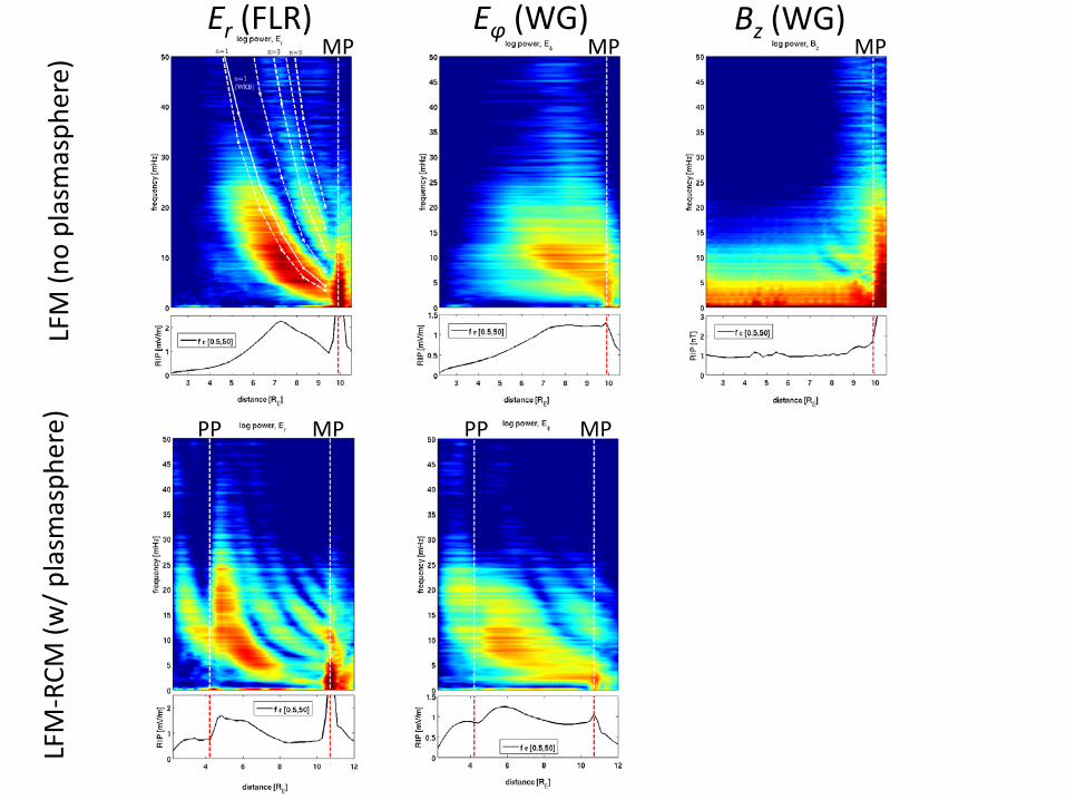
Er (FLR) Eφ (WG) Bz (WG)
MP MP MP
MP PP
Page 20
LFM
(no
plas
mas
pher
e)
LFM
-RCM
(w/ p
lasm
asph
ere)
Er (FLR) Eφ (WG) Bz (WG)
MP MP MP
MP MP PP PP
Page 21
LFM
(no
plas
mas
pher
e)
LFM
-RCM
(w/ p
lasm
asph
ere)
Er (FLR) Eφ (WG) Bz (WG)
MP MP MP
MP MP MP PP PP PP
Page 22
LFM-RCM (w/ plasmasphere)
Eφ (WG)
Bz (WG)
MP
MP PP
PP THEMIS Observations (statistical – all data from 2008)
Courtesy of Kazue Takahashi
Page 23
Figures courtesy of S. Ukhorskiy and D. Sibeck
4-8-12 hrs separation along 24 hour orbit
8-8-8
8-8-8
FS inner sphere Burst: PP, plume, EMIC
FS inner sphere Burst: Plume, EMIC, shock
FS inner sphere
FS plumes Burst: shocks FS, inner sphere waves
FS apogee, inbound Burst: dipolarization
FS inbound Burst: MS, chorus, EMIC
FS pp, outbound, apogee Burst dipol., pp, EMIC
THEMIS/RBSP Conjunction Campaigns
Page 24
Conclusions
• Solar wind dynamic pressure fluctuations can drive ULF waves on the dayside.
• Solar wind dynamic pressure fluctuations can excite toroidal mode FLRs and
compressional waveguide modes.
• First study of FLRs and waveguide modes using a global MHD model of the
solar wind/magnetosphere interaction.
• Recent work with the LFM-RCM, which includes a static plasmasphere, shows
promise for more detailed simulation/observation comparisons.
• The plasmasphere plays an important role in ULF wave generation in the inner
magnetosphere.