What Drives Sell-Side AnalystCompensation at High-

Status Investment Banks?The Harvard community has made this

article openly available. Please share howthis access benefits you. Your story matters

Citation Groysberg, Boris, Paul M. Healy, and David A. Maber. "What DrivesSell-Side Analyst Compensation at High-Status Investment Banks?"Journal of Accounting Research 49, no. 4 (2011): 969–1000.

Published Version doi:10.1111/j.1475-679X.2011.00417.x

Citable link http://nrs.harvard.edu/urn-3:HUL.InstRepos:13426865

Terms of Use This article was downloaded from Harvard University’s DASHrepository, and is made available under the terms and conditionsapplicable to Open Access Policy Articles, as set forth at http://nrs.harvard.edu/urn-3:HUL.InstRepos:dash.current.terms-of-use#OAP

WHAT DRIVES SELL-SIDE ANALYST COMPENSATION

AT HIGH-STATUS INVESTMENT BANKS?

Boris Groysberg*

Paul M. Healy**

Harvard Business School Harvard Business School

David A. Maber***

USC Marshall School of Business

This Draft:

March 29, 2011

This research was funded by the Division of Research at Harvard Business School and the USC Marshall School of

Business. We wish to thank I/B/E/S for analyst data and, especially, the anonymous financial services firms that

provided us with their financial analysts’ compensation data. We also wish to thank Alok Kumar, Douglas Emery,

and Xi Li, who generously supplied their Institutional Investor and WSJ star analyst data, and Malcolm Baker and

Jeffrey Wurgler for their market sentiment data. Helpful comments were provided by Doug Skinner (editor), an

anonymous reviewer, Mark Bagnoli, Jasmijn Bol, Sarah Bonner, Folkert Botma, Jan Bouwens, Mihir Desai, Pat

O’Brien, Fabrizio Ferri, Lee Fleming, Joseph Gerakos, Cam Harvey, Kai Li, Kevin J. Murphy, Steve Orpurt, Eddie

Riedl, Jenny Tucker, Susan Watts, Michael Welker, and seminar participants at the 2008 Ball & Brown Tribute

Conference at the University of New South Wales, 2008 CAAA Doctoral Consortium and 2009 CAAA Annual

Meeting, 19th

Annual Conference on Financial Economics and Accounting at the University of Texas at Austin,

2008 Financial Management Annual Meeting, 2008 London Business School Trans-Atlantic Doctoral Conference,

2008 Washington Area Finance Conference, 2009 FARS mid-year conference in New Orleans, Boston University,

Cornell, HBS, HKUST, Purdue, Singapore Management University, Tilburg, UBC, UNC, USC, and the University

of Technology, Sydney. The usual disclaimer applies.

* Email: bgroysberg@hbs.edu Phone: (617) 496-2784 Fax: (617) 496-6554

** Email: phealy@hbs.edu Phone: (617) 495-1283 Fax: (617) 496-7387

*** Email: maber@marshall.usc.edu Phone: (213) 740-1181 Fax: (213) 747-2815

WHAT DRIVES SELL-SIDE ANALYST COMPENSATION

AT HIGH-STATUS INVESTMENT BANKS?

ABSTRACT

We use proprietary data from a major investment bank to investigate factors associated with

analysts’ annual compensation. We find compensation to be positively related to “All-Star”

recognition, investment-banking contributions, the size of analysts’ portfolios, and whether an

analyst is identified as a top stock-picker by the Wall Street Journal. We find no evidence that

compensation is related to earnings forecast accuracy. But consistent with prior studies, we find

analyst turnover to be related to forecast accuracy, suggesting that analyst forecasting incentives

are primarily termination-based. Additional analyses indicate that “All-Star” recognition proxies

for buy-side client votes on analyst research quality used to allocate commissions across banks

and analysts. Taken as a whole, our evidence is consistent with analyst compensation being

designed to reward actions that increase brokerage and investment-banking revenues. To assess

the generality of our findings, we test the same relations using compensation data from a second

high-status bank and obtain similar results.

JEL Classification: G24, G29, J33, J44, L84, M41, M52

Keywords: Performance measurement, incentive compensation, financial analysts, Institutional

Investor ratings, investment banking.

1

1. Introduction

Sell-side research plays an important role in modern capital markets. Within the United

States, most top-tier investment banks spend in excess of one hundred million dollars annually

on equity research.1 Institutions and retail investors use equity research to help make investment

decisions (e.g., Madan, Sobhani, and Bhatia [2003]) and corporations rely on sell-side equity

analysts to market their securities and boost liquidity (e.g., Krigman, Shaw, and Womack

[2001]).

But because of limited access to data on analyst pay, prior studies’ assumptions about

analyst incentives are largely based on plausible conjectures rather than systematic evidence.

What little is known about analyst compensation is from the memoirs of former analysts (e.g.,

Reingold and Reingold [2006]) and a handful of stories on the reputed pay and characteristics of

well-known outliers like Jack Grubman, Mary Meeker, and Henry Blodget (e.g., Gasparino

[2005]). This paper uses analyst compensation data for the period 1988 to 2005 obtained from a

prominent integrated investment bank to formally examine analyst compensation and its drivers.2

Examining actual analyst compensation data enables us to test the incremental economic and

statistical significance of investment banking, brokerage, and other factors for analyst pay, and

thereby deepen our understanding of analysts’ financial incentives.

Our findings also shed light on the relationship between analyst compensation and the

two most studied measures of analyst performance, forecast accuracy and stock recommendation

profitability. Mikhail, Walther, and Willis [1999] and Hong and Kubik [2003] find analyst

1 The Sanford C. Bernstein estimates cited by Francis, Chen, Willis, and Philbrick [2004] imply that annual research budgets at

the top-8 investment banks averaged between $200 and $300 million during the 2000-2003 period. 2 Our sample bank is rated as “high status” or “top tier” based on a variety of criteria including the Carter-Manaster ten-tier

“tombstone” ranks provided in Carter, Dark, and Singh [1998], the size-based categorization provided in Hong, Kubik, and

Solomon [2000], and Institutional Investor’s annual buy-side polls.

2

forecast accuracy to be associated with job turnover and career prospects, suggesting an

association with compensation. But Mikhail et al. [1999] and Bradshaw [2008] note that this

relation is not based on actual evidence and conflicts with practitioner assertions that such factors

are not considered when making bonus awards.

We document several important facts, the first being large, systematic swings in the level

and skewness of real compensation throughout the 1988-2005 period. Median compensation

increased from $397,675 in 1994 to a peak of $1,148,435 in 2001, then declined to $647,500 in

2005. These ebbs and flows were highly correlated with swings in capital market activity, as

captured by the Baker and Wurgler [2006] market activity index. The increase in compensation

skewness was reflected in the ratio of analyst compensation at the 90th

and 10th

percentiles,

which was 2.6 in 1990, increased to 6.1 in 2000, and had declined to 4.0 by 2005. Variation in

the level and skewness of compensation over time was driven almost exclusively by bonus

awards, which grew from a low of 46% of total compensation in 1990 to 84% in 2002, and had

dropped to 70% by 2005. Collectively, the evidence indicates that during periods of high market

activity and correspondingly high trading commissions and corporate finance fees, a bank’s

bonus pool expands, leading to large increases in analyst compensation. But these large increases

are not shared equally among the bank’s analysts, as pay differentials also expand during “hot”

markets.

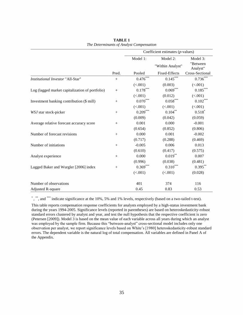
Second, most of the variation in analyst compensation can be explained by four factors,

(i) recognition by Institutional Investor (II) as an “All-Star” analyst, (ii) recognition by the Wall

Street Journal (WSJ) as a star stock-picker, (iii) an analyst’s investment-banking contributions,

and (iv) the size of an analyst’s portfolio. Pooled regressions that estimate the market level of

analyst pay based on observable characteristics indicate that, controlling for other hypothesized

3

determinants: II All-Star analysts earn 61% higher compensation than their unrated peers; top

stock-pickers, as recognized by the WSJ, earn about 23% more than their peers; analysts who

cover stocks that generate underwriting fees for their banks earn 7% higher pay for each million

dollars of fees earned; and the cross-sectional elasticity of compensation with respect to portfolio

size is approximately 0.18.

To evaluate pay-for-performance sensitivities (i.e., incentives), we follow the guidance in

Murphy [1985] and estimate analyst-fixed-effect regressions that rely on intra-analyst variation

in performance and compensation. These indicate that, controlling for other characteristics:

gaining (losing) II status is associated with a 16% compensation premium (penalty);

gaining/losing “star stock-picker” status in the WSJ is associated with an 11% change in pay;

covering stocks that generate underwriting fees for the bank is accompanied by 6% higher pay

for each million dollars of fees earned; and the intra-analyst elasticity of compensation with

respect to portfolio scale is just under 0.07.

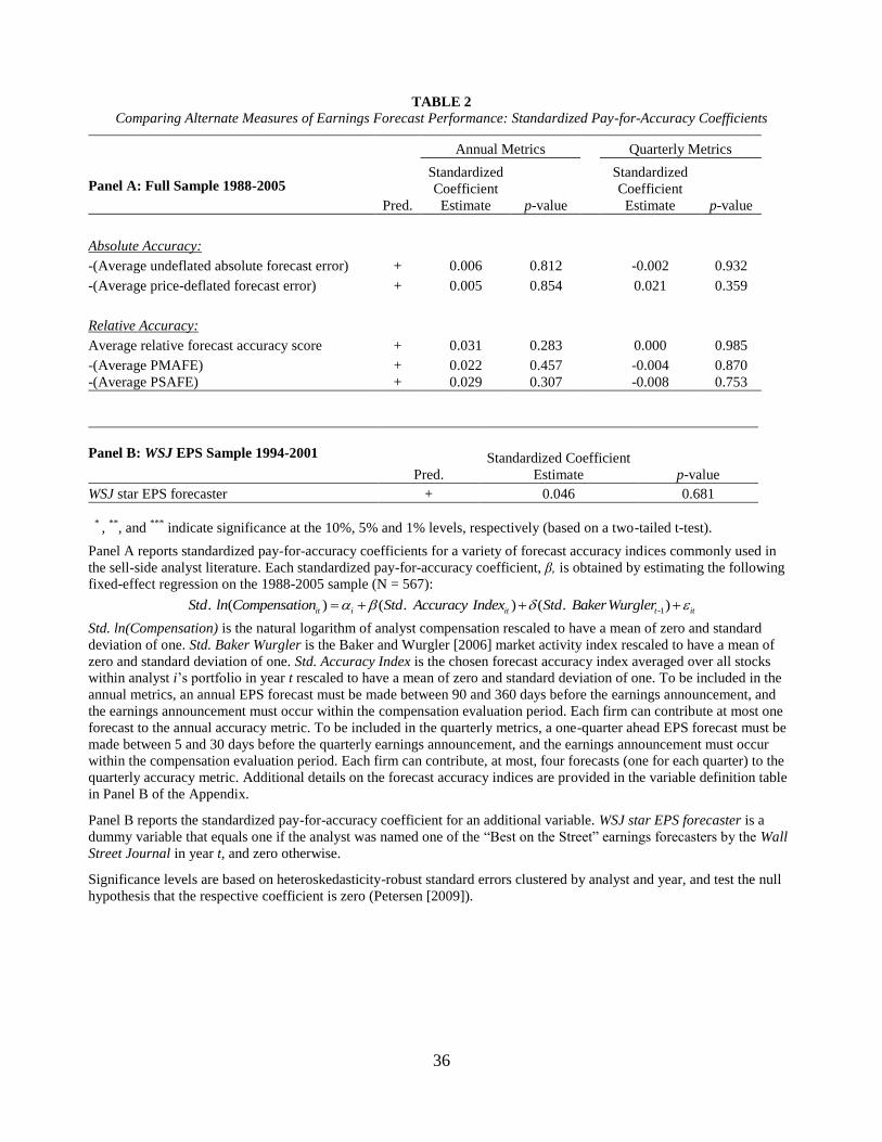
Third, for the sample firm’s analysts, forecast accuracy plays an insignificant role in

determining compensation. Interviews with equity research professionals at eleven large banks

(including the sample bank) as well as examination of the sample bank’s 2005 performance

evaluation and development booklet support this inference. It is unusual for large banks to

formally track forecast accuracy for compensation purposes. But we do find that inaccurate

analysts at the sample bank are more likely to move to lower-status banks or exit I/B/E/S, as

documented in the analyst turnover literature. “Fired” analyst-year observations had larger

forecast errors than other analysts who covered the same stocks and other analysts within the

sample firm. Taken as a whole, these findings suggest that forecasting incentives resemble a

Mirrlees contract. Under a normal range of forecasting outcomes, there is no relation between

4

forecasting performance and annual compensation within banks, but extremely adverse

forecasting outcomes are associated with increased probability of dismissal.3

Fourth, we find that much of the WSJ “star stock-picker” compensation premium appears

to reflect public recognition, not underlying stock-picking performance. Moreover, the

association between underlying stock-picking performance and compensation occurs with a one-

year lag, reflecting the timing of the WSJ report. We conclude that stock-picking performance

affects analyst compensation, but the effect is delayed and only economically significant if it

boosts an analyst’s visibility. Discussions during our interviews support this inference. Although

stock-picking performance is commonly tracked as part of banks’ analyst evaluation and

development processes, insiders indicated that it generally is not a major determinant of analyst

compensation.

Finally, we find that the II compensation premium can be explained by the underlying

votes of institutional investors (i.e., the “buy-side”), which closely approximate the “broker

votes” used to allocate commissions across banks and analysts. Controlling for institutional

investors’ votes, the relation between compensation and “All-Star” rating in II becomes

economically and statistically insignificant. In other words, the association between

compensation and II-status does not appear to be attributable to the added visibility associated

with being assigned star status in II’s October issue.

Our findings are robust to a battery of tests including alternative definitions of key

variables, alternative measurement windows, sample-selection controls, first differencing (i.e.,

“changes”), and replication using data from a second high-status investment bank. Interviews

with research directors at other leading banks indicated remarkable consistency in the

3 See Bolton and Dewatripont [2005] and Christensen and Feltham [2005] for a discussion of Mirrlees contracts and the

“Mirrlees Problem.”

5

performance metrics used to determine analyst bonus awards, suggesting that our findings are

likely to hold for other top-tier banks as well.

We nevertheless caution readers against generalizing our findings to non-representative

settings. In particular, it seems highly unlikely that they will apply to lower-status banks or

brokerage firms that employ few if any II-ranked analysts and do not generate substantial

investment banking revenues. We further recognize that the importance of investment banking to

analyst compensation is likely to diminish following the Global Settlement. But we are unable to

test this hypothesis given restrictions imposed by our sample firm and the limited number of

post-settlement observations.

The paper is organized as follows. Section 2 describes the proprietary and public data

used in the study. Section 3 provides summary information on analyst compensation. Section 4

discusses the hypothesized drivers of analyst compensation. Empirical results are presented in

Sections 5 and 6. Section 7 concludes with a discussion of results and suggestions for future

research.

2. Data

The data used in this study were obtained from a proprietary compensation file and five

publicly available sources: I/B/E/S, CRSP, SDC Platinum, Institutional Investor, and the Wall

Street Journal. The proprietary compensation file is based on a set of spreadsheets obtained from

a leading Wall Street investment bank for the years 1988-2005. The spreadsheets report the

name, hire date, and compensation of each of the bank’s analysts. No other variables are

contained in these spreadsheets.

The bank’s senior research staff also provided marked-up photocopies of the research

director’s 2005 analyst evaluation and development booklet. This booklet reports analyst

6

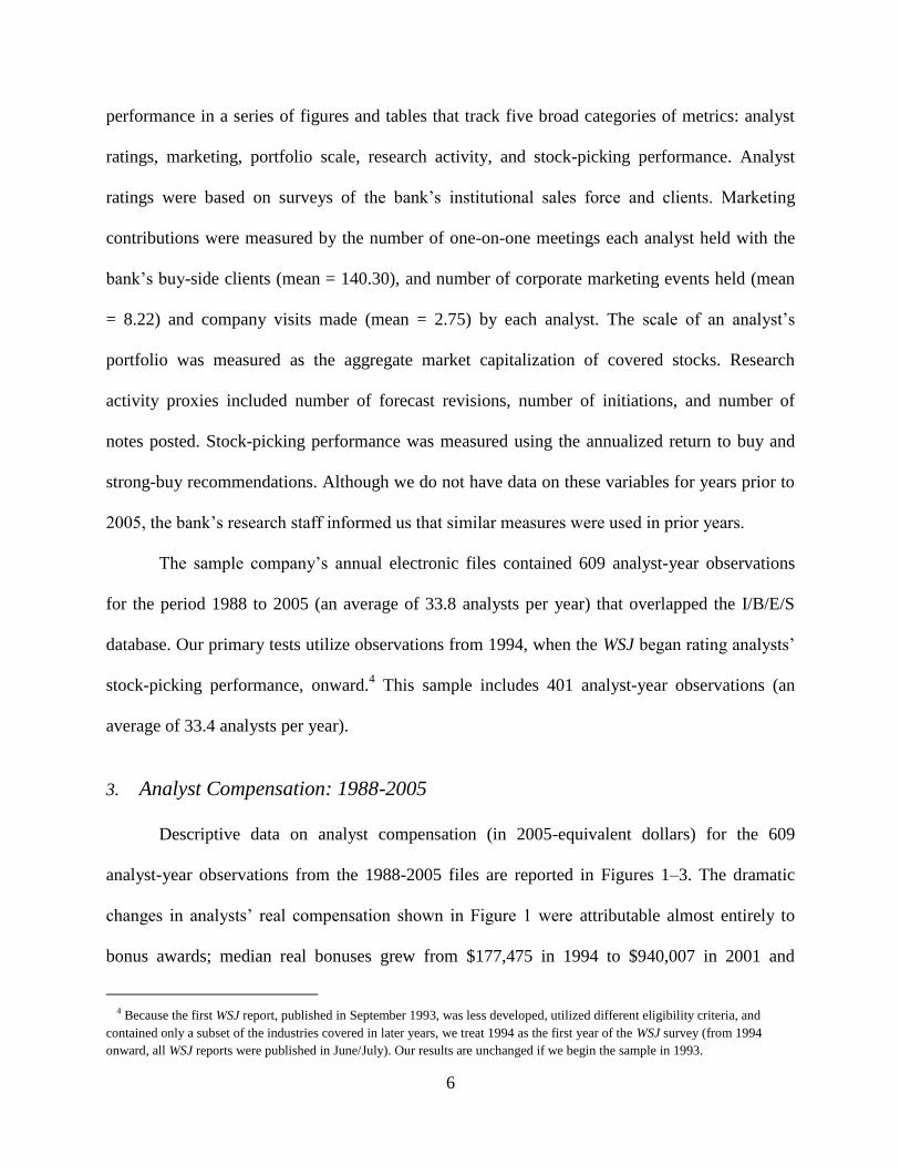
performance in a series of figures and tables that track five broad categories of metrics: analyst

ratings, marketing, portfolio scale, research activity, and stock-picking performance. Analyst

ratings were based on surveys of the bank’s institutional sales force and clients. Marketing

contributions were measured by the number of one-on-one meetings each analyst held with the

bank’s buy-side clients (mean = 140.30), and number of corporate marketing events held (mean

= 8.22) and company visits made (mean = 2.75) by each analyst. The scale of an analyst’s

portfolio was measured as the aggregate market capitalization of covered stocks. Research

activity proxies included number of forecast revisions, number of initiations, and number of

notes posted. Stock-picking performance was measured using the annualized return to buy and

strong-buy recommendations. Although we do not have data on these variables for years prior to

2005, the bank’s research staff informed us that similar measures were used in prior years.

The sample company’s annual electronic files contained 609 analyst-year observations

for the period 1988 to 2005 (an average of 33.8 analysts per year) that overlapped the I/B/E/S

database. Our primary tests utilize observations from 1994, when the WSJ began rating analysts’

stock-picking performance, onward.4 This sample includes 401 analyst-year observations (an

average of 33.4 analysts per year).

3. Analyst Compensation: 1988-2005

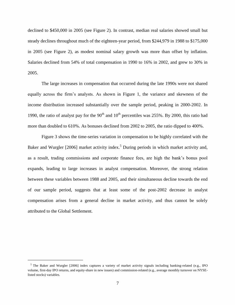
Descriptive data on analyst compensation (in 2005-equivalent dollars) for the 609

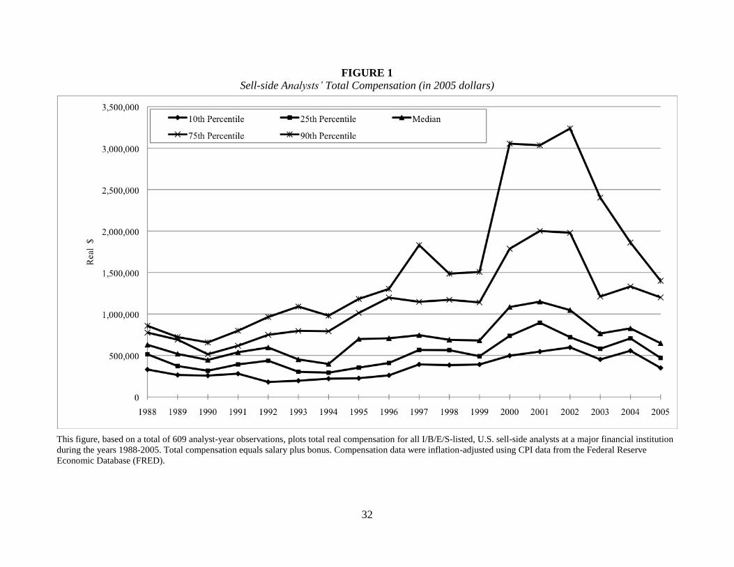
analyst-year observations from the 1988-2005 files are reported in Figures 1–3. The dramatic

changes in analysts’ real compensation shown in Figure 1 were attributable almost entirely to

bonus awards; median real bonuses grew from $177,475 in 1994 to $940,007 in 2001 and

4 Because the first WSJ report, published in September 1993, was less developed, utilized different eligibility criteria, and

contained only a subset of the industries covered in later years, we treat 1994 as the first year of the WSJ survey (from 1994

onward, all WSJ reports were published in June/July). Our results are unchanged if we begin the sample in 1993.

7

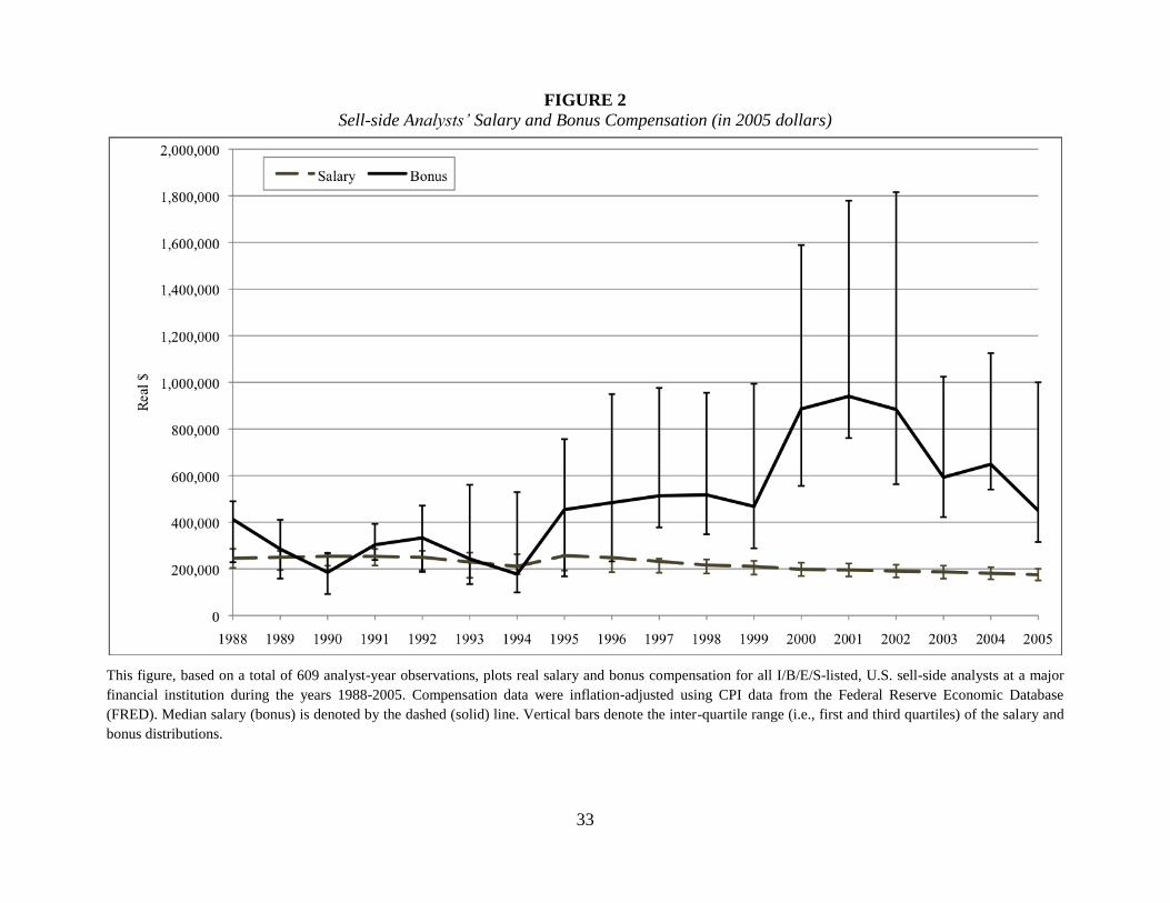
declined to $450,000 in 2005 (see Figure 2). In contrast, median real salaries showed small but

steady declines throughout much of the eighteen-year period, from $244,979 in 1988 to $175,000

in 2005 (see Figure 2), as modest nominal salary growth was more than offset by inflation.

Salaries declined from 54% of total compensation in 1990 to 16% in 2002, and grew to 30% in

2005.

The large increases in compensation that occurred during the late 1990s were not shared

equally across the firm’s analysts. As shown in Figure 1, the variance and skewness of the

income distribution increased substantially over the sample period, peaking in 2000-2002. In

1990, the ratio of analyst pay for the 90th

and 10th

percentiles was 255%. By 2000, this ratio had

more than doubled to 610%. As bonuses declined from 2002 to 2005, the ratio dipped to 400%.

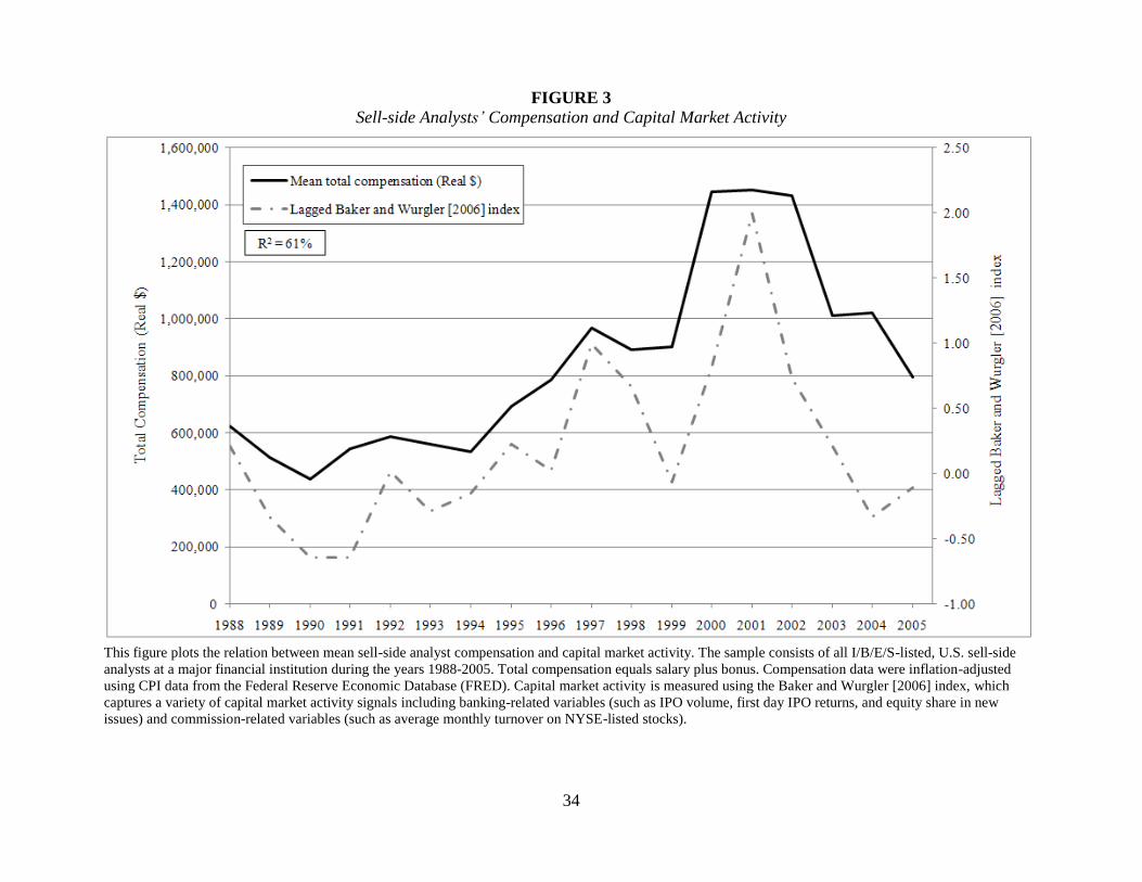
Figure 3 shows the time-series variation in compensation to be highly correlated with the

Baker and Wurgler [2006] market activity index.5 During periods in which market activity and,

as a result, trading commissions and corporate finance fees, are high the bank’s bonus pool

expands, leading to large increases in analyst compensation. Moreover, the strong relation

between these variables between 1988 and 2005, and their simultaneous decline towards the end

of our sample period, suggests that at least some of the post-2002 decrease in analyst

compensation arises from a general decline in market activity, and thus cannot be solely

attributed to the Global Settlement.

5 The Baker and Wurgler [2006] index captures a variety of market activity signals including banking-related (e.g., IPO

volume, first-day IPO returns, and equity-share in new issues) and commission-related (e.g., average monthly turnover on NYSE-

listed stocks) variables.

8

4. Drivers of Compensation

In this section, we draw on results from the human capital acquisition, job assignment, and

principal agent (i.e., incentive contracting) literatures to categorize the determinants of analyst

compensation.6 Traditional models of human capital acquisition and job assignment (e.g., Mayer

[1960], Becker [1964], and Rosen [1982]) predict that compensation will be increasing in

experience and the value of assets under an employee’s control. These predictions follow from

three assumptions, (i) productive talent is a scarce resource, (ii) productivity is increasing in

experience and innate ability, and (iii) the marginal impact of workers’ talent is increasing in the

value of assets under their control, implying that only the most talented employees will be

assigned to large, complicated, portfolios of tasks.

Traditional treatments of the principal-agent problem predict that “action-based” (that is,

high signal-to-noise ratio) performance measures will be used extensively, as they allow stronger

incentives without requiring a high risk premium for the employee (e.g., Banker and Datar

[1989]). As noted by Baker [2002], however, action-based measures are “narrow” or

“incomplete,” potentially providing distorted incentives (i.e., if overemphasized, they incentivize

the wrong behavior). “Outcome-based” performance measures, on the other hand, typically

provide greater goal-congruence but require a higher risk premium for the employee. Moreover,

in complex production environments in which each action’s marginal product is state-contingent,

tying their rewards to outcome-based measures provides employees with stronger incentives to

utilize non-contractible (i.e., tacit), state-specific knowledge (Prendergast [2002], Baker and

Jorgensen [2003], and Raith [2008]).

6 See Milgrom and Roberts [1992], Gibbons and Waldman [1999], and Prendergast [1999] for reviews of these literatures.

9

We use these insights to frame our investigation of the determinants of sell-side analyst

compensation. Our choice of compensation determinants also is guided by the sample bank’s

2005 analyst evaluation and development booklet as well as field interviews at eleven investment

banks and prior analyst research.

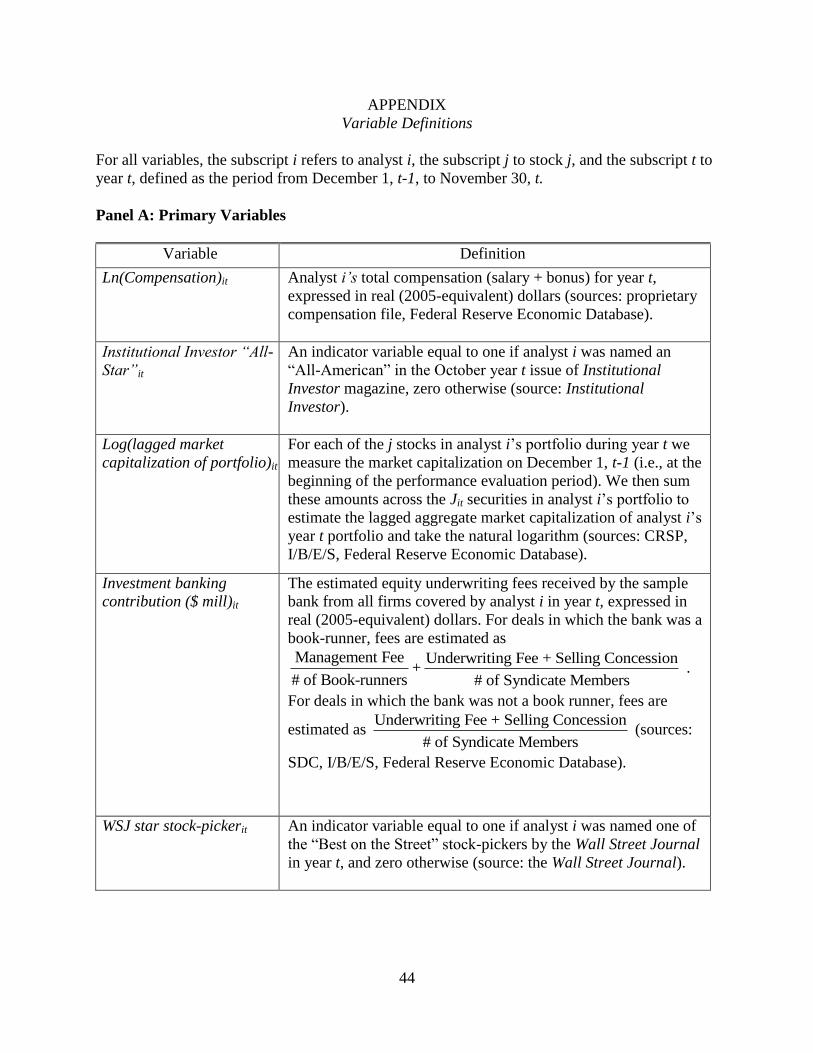
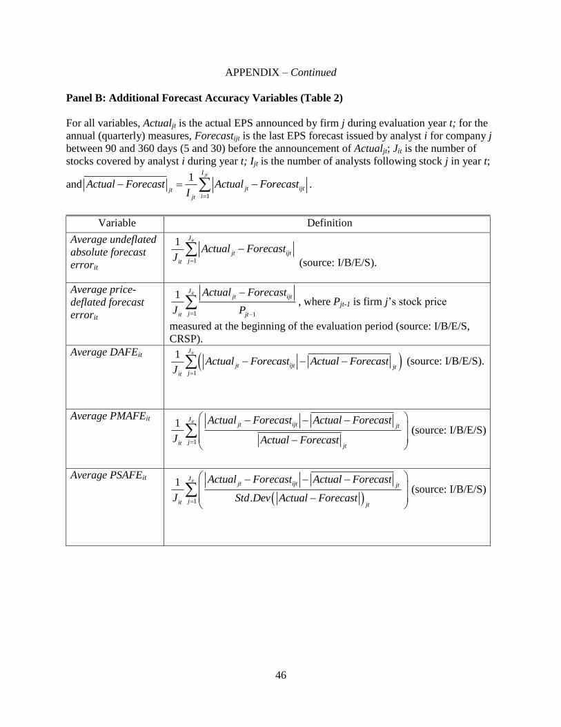
In assembling our variables, which are defined in the Appendix, we ensured that the

measurement intervals were consistent with the timing of compensation awards. Each variable’s

outcome is realized prior to the compensation award date, and therefore is a potential input to the

compensation decision.

4.1. OUTCOME-BASED PERFORMANCE VARIABLES

Institutional Investor Ratings. Since 1972, Institutional Investor (II) has conducted

annual surveys of buy-side institutions’ ratings of sell-side analysts who “have been the most

helpful to them and their institution in researching U.S. equities over the past twelve months”

(Institutional Investor [1996, 1997]). Based on these surveys, a list of the top-three analysts and

runners-up by industry is published in the magazine’s October issue. “All-Star” ratings are

widely viewed as the most comprehensive public measure of analyst performance (e.g.,

Bradshaw [2008]). We construct an II All-Star indicator variable that takes the value one if an

analyst at the sample firm is named by II as one of the top-three analysts or a runner-up in a

given year, and zero otherwise.

Prior research suggests that All-Star analysts contribute to the performance of their

investment banks by generating higher trading volumes (Jackson [2005]) and attracting

investment-banking clients (Dunbar [2000], Krigman et al. [2001], and Clarke, Khorana, Patel,

and Rau [2007]). Among higher-status banks, II-ratings are likely to be highly correlated with

client votes on the quality of analysts’ research that are used to allocate transactions and, hence,

10

commissions among banks. Data from the research director’s 2005 performance-evaluation

booklet indicates that among the ten analysts with the highest client votes, eight were II-rated

(none of the ten analysts with the lowest client votes were II-rated).7

Firm management and practitioners stated that banks prefer to tie analyst compensation,

when available, to client votes (as opposed to the trading volumes and commissions of covered

stocks). According to these insiders, client votes incorporate the impact of important externalities

and better reflect an analyst’s contribution to total (i.e., bank-wide) commission revenue. First,

votes are not as affected by the quality of a bank’s traders. Further, an analyst’s research on a

stock can lead clients to continue holding the security and, hence, not affect trading. Yet clients

that value such research typically reward the bank for the research by allocating it trading

commissions on other stock transactions. Consistent with these arguments, O’Brien and Bhushan

[1990, p. 59] observe that “it is rare (and controversial) for research analysts’ compensation to be

explicitly based on commissions.”

Investment-Banking Contribution. Our second outcome-based performance measure is

the analyst’s contribution to the bank’s investment-banking operations. Analysts contribute to

investment-banking deals by identifying potential issuers, providing investors with valuable

information about issuers, and participating in road shows to sell issues to institutional clients.

For each analyst-year, our primary banking variable is the annual equity underwriting fees

earned by the bank from the companies an analyst covered. Since the fees received by each bank

are not publicly disclosed, we estimate the banking fees received from each deal using the

following algorithm: the management fee, which typically accounts for 20% of the gross spread,

7 Fisher’s exact test indicates this association to be statistically significant at the 1% level.

11

is divided equally among the book-runners, and the underwriting fee and selling concessions are

divided equally among all syndicate members.8

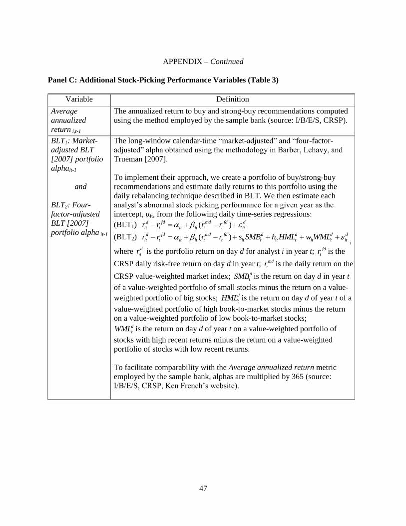
Stock Recommendation Performance. Prior research suggests that (changes in) stock

recommendations have investment value for bank clients (Womack [1996], Irvine [2004],

Jegadeesh, Kim, Krische, and Lee [2004], Green [2006], Juergens and Lindsey [2009]). Analysts

with superior recommendation performance potentially create value by enhancing a bank’s

reputation in the WSJ’s research ratings, which are based solely on recommendation

performance, and by generating commission revenues from clients who value their research.

Many of the research directors we interviewed indicated that they track analysts’

recommendation performance, and anecdotal evidence suggests that investment banks care about

the WSJ’s ratings. For example, Merrill Lynch posted on its Web site the names of its nine

analysts who made the 2005 WSJ rankings, and the head of its Americas Equity Research

commented on the bank’s strong ranking (Merrill Lynch [2005]).

Our primary measure of stock-picking ability is an indicator variable that takes the value

one if the WSJ’s annual ratings identified the analyst as one of the top-five stock pickers in his or

her industry, and zero otherwise.9 In Section 6.2 we also examine the mean annualized raw

return to buy and strong-buy recommendations, the approach used by the sample firm to measure

recommendation performance. This measure is constructed by scaling the return to each buy and

8 This simple algorithm assumes an equal allocation across syndicate members. Although we are unaware of any research on

SEO allocations, research on IPO allocations using proprietary data indicates that book-runners typically receive a larger share

allocation (see Iannotta [2010] for a review of this literature). Consequently, we also estimated equity underwriting fees by

dividing total fees by the number of book-runners. This approach implicitly assumes that a deal’s book-runners were allocated

100% of the shares in the equity underwriting process. Our results are robust to this alternate fee estimation algorithm (see

Section 6.4). 9 To be eligible, an analyst must cover five or more qualified stocks in the industry (i.e., stocks that trade above $2/share and

have a market cap of more than $50 million), and at least two of the qualified stocks must be among the ten largest stocks in the

industry (the theory is that no one can truly understand an industry without a thorough knowledge of at least some of its biggest

firms). As noted by Emery and Li [2009], these eligibility conditions are generally non-binding for analysts at larger brokerage

houses, such as the bank studied here, and, conditional on eligibility, the ratings are entirely determined by stock-picking

performance.

12

strong-buy recommendation by the number of days a stock is held relative to the number of days

in the year. For example, if a buy recommendation generates a return of 7% for 60 days, the

annualized return is 43% (7%*365/60).

Earnings Forecast Accuracy. Research on analysts’ earnings forecasts finds more

accurate forecasting to be associated with “favorable” job transitions (Mikhail et al. [1999] and

Hong and Kubik [2003]) and top-tier investment banks to employ significantly more accurate

forecasters (e.g., Clement [1999], Malloy [2005], and Cowen, Groysberg, and Healy [2006]). It

thus appears that prestigious Wall Street research houses like our sample firm demand forecast

accuracy.

As discussed in Section 6.1, forecast accuracy was not formally tracked in the 2005

performance evaluation and development booklet received from the sample bank. Consequently,

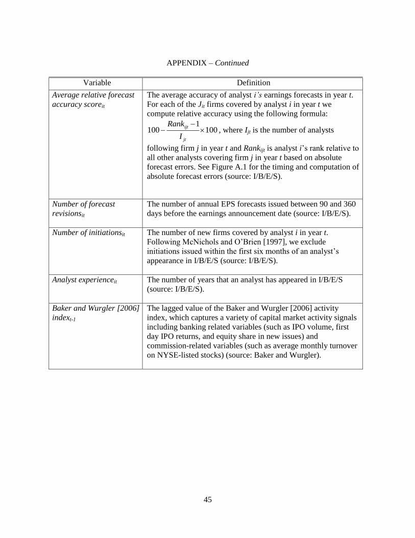
we rely on prior literature to guide our choice of a forecast accuracy index. We use analysts’

most recent annual earnings forecasts issued from 360 to 90 days prior to annual earnings

announcements that fall within the compensation evaluation period.10,11

Following Gu and Wu

[2003] and Basu and Markov [2004], we compute absolute (as opposed to squared) forecast

errors for each analyst-firm-year. These unsigned errors are aggregated into a single relative

performance score using the following formula:1

100 100ijt

jt

Rank

I

, where Ijt is the number of

analysts following firm j in year t and Rankijt is analyst i’s accuracy rank relative to all other

analysts covering firm j in year t (see Hong and Kubik [2003] and Ke and Yu [2006]). Lastly, we

10 Prior studies of analyst incentives use annual (as opposed to quarterly) earnings forecasts (e.g., Hong and Kubik [2003], Ke

and Yu [2006], Leone and Wu [2007], Ertimur, Mayew, and Stubben [2008], and Call, Chen, and Tong [2009]) and the most

recent forecast issued (e.g. O’Brien [1990], Clement [1999], Jacob, Lys, and Neale [1999], Mikhail et al. [1999], Hong and

Kubik [2003], and Ke and Yu [2006]). 11 Our results are robust to alternate windows including 10-90 days before the announcement, 90-180 days before the

announcement, 180-270 days before the announcement, and 270-360 days before the announcement. We obtain similar results

when we control for length of the forecasting horizon.

13

average the relative scores over all companies covered by an analyst within a performance-

evaluation year.12

4.2. ACTION-BASED PERFORMANCE MEASURES

Earnings Forecast Update Frequency. This measure was included in the 2005

performance evaluation and development booklet received from our sample bank and widely

tracked by other banks we interviewed. It also is the most widely used action-based performance

measure in the analyst literature. Jacob et al. [1999], Mikhail, Walther and Willis [2009], and

Pandit, Willis, and Zhou [2009] use it as a proxy for analyst effort, which theory predicts should

be strongly associated with incentive compensation (e.g., Holmström [1979]). Moreover, prior

research suggests that this variable is a leading indicator of investment-banking revenues.

Krigman et al. [2001], for example, find dissatisfaction with frequency of coverage to be a key

determinant of firms’ decisions to switch underwriters. Finally, frequent revisions may generate

abnormal commission revenue (e.g., Juergens and Lindsey [2009]).

We compute earnings estimate update frequency as the number of annual forecasts issued

by an analyst each year during the 360 to 90 days prior to a covered company’s EPS

announcement (broadly similar to the approach used in Hong et al. [2000]).

Coverage Initiations. Our second action-based performance measure is the number of

coverage initiations made by an analyst. Initiations were widely tracked by the banks we

interviewed, appeared in the sample firm’s 2005 performance evaluation and development

booklet, and have been the subject of prior academic research. Ertimur, Muslu, and Zhang [2007]

and Bradshaw, Richardson, and Sloan [2006], for example, cite anecdotes that suggest that

analysts may be compensated on the basis of initiation frequency.

12 Following Jacob et. al. [1999], Ke and Yu [2006], and others, we drop companies for which Ijt < 3 because relative

performance isn’t meaningful in such situations.

14

4.3. JOB CHARACTERISTICS

Portfolio Scale. Research directors we interviewed indicated that it is particularly

important to have strong analysts cover large, highly traded stocks that have a disproportionate

impact on the business. Their claim is supported by large-sample evidence in Hong and Kubik

[2003] and a recent Sanford C. Bernstein report (Hintz, Werner, and St. John [2006]) that argues

that analysts who cover large portfolios are more visible, generate greater commissions, and are

allocated a large share of the firm’s research resources. Because banks bid aggressively for the

services of analysts with the requisite skill to cover these portfolios, we expect a positive

association between portfolio scale and compensation.

Consistent with the sample bank, we measure portfolio scale as the aggregate market

capitalization of covered stocks.13

To ensure that we capture scale and not the performance of

covered stocks, we measure the market capitalization of each stock covered during year t at the

beginning of the performance-evaluation period (i.e., December 1st, t-1). Finally, to facilitate

interpretation of the pay-scale relation, we take the natural logarithm of our portfolio scale proxy.

Consequently, our regression parameters can be interpreted as the partial elasticity of pay with

respect to portfolio size (e.g., Rosen [1992]).

4.4. HUMAN CAPITAL CHARACTERISTICS

Experience. If analysts learn important tasks like mentoring through experience, and these

benefits are not fully captured in our outcome- and action-based measures of performance, we

should find a positive association between analyst compensation and experience. Equivalently,

experience can be viewed as a control for unobservable performance variables. In our tests,

13 We obtain a similar, albeit weaker, association when we substitute number of stocks covered for market capitalization. When

we include both market capitalization and number of stocks covered, only the market capitalization of covered stocks is

economically or statistically significant in our model.

15

analyst experience is defined as the number of years an analyst has been employed as a senior

analyst.14

To preserve the sample firm’s anonymity, we do not report descriptive statistics for its

analysts on the explanatory variables described above. However, unreported tests show the

sample analysts to be indistinguishable from their peers at other top-20 rated firms in terms of II

rating, experience, forecast accuracy, strong-buy/buy recommendation performance, portfolio

scale, number of firms covered, and annual number of forecast revisions and stock initiations

issued.

5. Main Results

Following other compensation studies and guided by Rosen [1992], we use logarithmic

regressions to estimate the implicit weights the sample firm’s compensation system places on

various measures. Compensation response coefficients are estimated using total direct

compensation for the period 1994 to 2005. We estimate three models, (i) a pooled model, (ii) a

“within-analyst” fixed-effects model, and (iii) a “between-analyst” cross-sectional model.

Significance levels for the first two models are based on heteroskedasticity-robust standard errors

clustered by analyst and year (Petersen [2009]). Because the between-analyst cross-sectional

model includes only one observation per analyst, we report significance levels based on White’s

[1980] heteroskedasticity-robust standard errors. To control for the effects of general market

movements documented in Figure 3, we include in our regression models lagged values of the

Baker and Wurgler [2006] index. Our results are quantitatively and qualitatively similar when we

substitute for this index a set of year indicator variables.

14 Experience, as noted by Clement, Koonce, and Lopez [2007], is a broad concept, and different types of experience can be

associated with different types of human capital. Our definition of experience is similar to Clement’s [1999] in that it captures

analysts’ experience within the profession (as opposed to experience covering specific stocks, events, or transactions).

16

5.1. POOLED MODEL

The first column of Table 1 presents results for our pooled total compensation model.

The estimated coefficients indicate that four variables (in addition to the market activity index)

have economically and statistically significant associations with analyst pay: All-Star status;

portfolio scale; investment-banking contributions; and recognition by the WSJ as a star stock-

picker. The coefficients for forecast accuracy, number of forecast revisions, number of stock

initiations, and analyst experience are statistically indistinguishable from zero.

The estimated All-Star coefficient of 0.476 implies that, on average, total compensation

of All-Star analysts was 61% higher than that of non-star analysts, holding other factors

constant.15

The parameter estimate on our portfolio scale variable, the natural logarithm of the

lagged market capitalization of covered stocks, is 0.178, implying that an analyst whose portfolio

is at the third market capitalization quartile earned approximately 41% higher total compensation

than a peer who covered a portfolio at the first market capitalization quartile, holding other

factors constant. The investment-banking coefficient of 0.070 indicates that, on average, an

analyst who generates $1 million in banking-related revenue will earn 7% more compensation

than a peer with no banking contributions, holding other factors constant. Finally, the 0.209 WSJ

coefficient indicates that analysts whose stock-picking performance is formally recognized by

the WSJ earn approximately 23% more than their unranked peers, holding other factors constant.

5.2. FIXED-EFFECTS MODEL

As noted by Murphy [1985], in a pooled compensation regression the explanatory

variables may be correlated with unobservable factors (such as talent/ability) that are the real

15 A one-unit change in the explanatory variable X is associated with a 100 ∙ (eb – 1)% change in compensation, where b

denotes the estimated coefficient on variable X.

17

drivers of compensation. A common approach to dealing with this concern is to use a fixed-

effects model. Wooldridge [2002], among others, has shown a fixed-effect specification to

provide consistent parameter estimates if choices (i.e., assignment or selection) are a function of

the unobservable fixed-effects. Including analyst fixed-effects in our compensation model

controls for time-invariant cross-sectional differences in analyst ability, which enables us to

examine whether “within-analyst” variation in our explanatory variables (e.g., II ranking,

investment-banking contributions) is related to “within-analyst” variation in compensation.16

The results of the fixed-effects model are reported in the second column of Table 1.

Because fixed-effects require at least two observations for each analyst, sample size declines

from 401 to 374 analyst-year observations. Similar to our pooled results, we find four variables

to be highly associated with compensation: All-Star status; portfolio scale; investment-banking

transactions by covered firms; and star stock picking. The All-Star coefficient of 0.145 implies

that gaining (losing) II status is accompanied by a 16% compensation premium (penalty). In

unreported tests, we are unable to reject the hypothesis that the percentage increase in

compensation from gaining All-Star status equals the percentage decrease in compensation from

losing All-Star status. This fixed-effect estimate is considerably smaller than that obtained from

our pooled model (61%). There are two potential explanations for this difference. First, if All-

Star status and analyst ability are correlated, some of the All-Star effect from the pooled model

will be subsumed in the analyst fixed-effect. A second explanation is that a compensation

premium accrues to star analysts who are ranked highly year after year. This premium is

16 As an alternative to fixed-effects, some compensation studies employ first-differences (i.e., “changes”). As noted by

Wooldridge [2002] and Cameron and Trivedi [2005], when the number of time periods equals 2, both estimators are equivalent.

When T > 2 and the model is well specified, both estimators are unbiased and consistent. Consequently, differences between the

estimators will reflect differences in efficiency. Which estimator is more efficient depends on the structure of the time-variant

disturbance term. If the time-variant disturbance term approximates a random walk, first-differences are more efficient; if it is

serially uncorrelated, fixed-effects are more efficient. In most cases, the truth lies somewhere in between. Thus, as a robustness

test, we repeated each of our analyses using first-differences. Our inferences were unchanged.

18

reflected in pooled estimates, but not in the fixed-effect model because it is unusual for analysts

who have been ranked for a number of years to lose their ranking.

The portfolio scale elasticity estimate of 0.069 implies that the compensation of analysts

who increase the scale of their portfolio by 10% will increase, on average, by less than 1%.

Although statistically significant, this estimated coefficient is considerably smaller than the

corresponding figure from the pooled regression, indicating that the pooled compensation-scale

relation partially reflects the matching of more talented analysts to larger portfolios of stocks

(i.e., pay for ability). This result is consistent with the job characteristics literature prediction that

highly talented analysts will be sought to cover economically important industries/portfolios of

stocks and their high pay will reflect a scarcity rent. According to the theory, compensation and

portfolio scale are jointly determined by (unobservable) abilities.

Our fixed-effect estimates indicate that gaining or losing star stock-picker status in the

WSJ is associated with an 11% change in pay. We are unable to reject the hypothesis that the

percentage increase in compensation from gaining WSJ recognition equals the percentage

decrease in compensation from losing WSJ recognition. Note that whereas the II coefficient from

the fixed-effects model is only 30% as large as the corresponding pooled coefficient, the WSJ

coefficient from the fixed-effects model is 50% as large as the corresponding pooled estimate.

This finding is consistent with evidence reported by Emery and Li [2009] that WSJ stock-picking

ratings are considerably less persistent than II ratings (the year-to-year probability of retaining II

status is approximately 0.7, the year-to-year probability of retaining WSJ status around 0.2).

The fixed-effect estimate for investment banking is 0.058, similar to the pooled estimate.

Estimates for the remaining variables – forecast accuracy, forecast revisions, stock initiations,

and experience – are insignificantly different from zero.

19

5.3 “BETWEEN-ANALYST” CROSS-SECTIONAL MODEL

Our third model uses the average values of compensation and independent variables

during each analyst’s employment with the sample firm. By including each analyst in the sample

only once, this approach controls for any dependence among analyst observations (Greene

[2000]).17

More important, it mitigates any timing mismatches (i.e., lead/lag issues) in our

independent variables, and indicates whether consistently strong performance is rewarded with

greater pay over an analyst’s tenure. Finally, it provides a bridge between the pooled model and

“within-analyst” fixed-effect model, as it represents the variation in the pooled model that has

been purged from the fixed-effect model (Murphy [1985], Greene [2000], Verbeek [2005]).

The findings reported in the third column of Table 1 indicate that analyst compensation is

related to the same four analyst characteristics. Not surprisingly, the estimates are typically much

larger than those reported for the “within-analyst” fixed-effect model. For example, the II All-

Star estimate of 0.736 implies that, on average, analysts rated as All-Stars consistently

throughout their employment at the sample firm earned 109% higher compensation than analysts

who were never rated.

6. Additional Analyses

6.1. FORECAST ACCURACY

Finding no economically or statistically significant association between forecast accuracy

and compensation is somewhat surprising given prior evidence that forecast accuracy is related

to analysts’ career prospects (see Mikhail et al. [1999] and Hong and Kubik [2003]). But it is

consistent with the inferences from our interviews at eleven leading banks, and the fact that the

research director’s 2005 analyst evaluation and development booklet did not track analysts’

17 Given that we report significance levels based on 2-way clustered standard errors, our pooled and fixed-effect models should

not be affected by dependence among analyst observations (Petersen [2009]).

20

forecasting performance. When asked about this omission, the bank’s research director

remarked: “I have never tracked it and nowhere that I have been did before I arrived. I don't

think it is any kind of acid test for whether an analyst has keen insight. If the clients pay attention

to and pay for the services of an analyst, then that is a ‘good’ analyst, whether or not they get the

earnings, or for that matter, stock prices, right.”

The fact that forecast accuracy was excluded from the bank’s analyst evaluation and

development documents presents strong evidence that forecast accuracy is not a direct

determinant of analyst compensation. It is possible, though, that forecast accuracy is implicitly

rewarded through other mechanisms, such as II ratings. Consequently, in this section we provide

additional analyses of analysts’ forecasting incentives, and examine whether the lack of

association documented in Table 1 is an artifact of our research design.

6.1.1. Noisy Forecast Accuracy Measure, Correlated Regressors, and Small Sample Size. To

investigate whether our findings are sensitive to the forecast accuracy metric employed, we

construct four other forecast accuracy metrics that are popular in the analyst literature, (i)

undeflated absolute forecast errors, (ii) price-deflated absolute forecast errors, (iii) the

proportional mean absolute forecast error (PMAFE) metric reported in Clement [1999], Jacob et

al. [1999], and Clement et al. [2007], and (iv) the standard-deviation-deflated measure (PSAFE)

reported in Groysberg, Healy, and Chapman [2008].18

Each of these metrics is estimated using

both annual and quarterly forecast data from I/B/E/S. Definitions are reported in Panel B of the

Appendix. In addition to these I/B/E/S-based metrics, we use an indicator variable that takes the

value one if the WSJ’s annual ratings identified the analyst as one of the top-five forecasters in

18 In unreported analyses, we examine forecast metrics for the most recent two and three years (as opposed to the most recent

year); year-to-year changes in forecast accuracy, as opposed to the level of forecast accuracy; the first (as opposed to last)

forecast within the forecast window; squared, as opposed to absolute, forecast errors; and analysts’ median, as opposed to mean,

forecast accuracy.

21

his or her industry, and zero otherwise.

To ensure that the relation between compensation and forecast accuracy is not subsumed by

other regressors, we exclude all other variables from the model except the lagged Baker and

Wurgler index that controls for exogenous variation in the bank’s bonus pool. For tests involving

the I/B/E/S-based forecast accuracy metrics, dropping these variables also enables us to utilize

the larger 1988-2005 sample, thereby increasing the power of our tests.

Pay-for-accuracy coefficients are estimated for each forecast accuracy measure as well as for

the average relative forecast accuracy score used above. To compare the parameter estimates for

these variables given their scale differences (e.g., average undeflated forecast errors are reported

in cents and the forecast accuracy index is a 0-100 relative scale), we standardize the

compensation and explanatory variables to have zero mean and unit standard deviation. The

estimated coefficients then indicate how a one standard deviation change in forecast accuracy

affects compensation (in standard deviations).

Panel A of Table 2 reports standardized coefficients for the I/B/E/S-based accuracy metrics.

The results indicate that the weak pay-for-accuracy relation documented in Table 1 is not an

artifact of the forecast metric used, the inclusion of other (potentially correlated) variables, or the

smaller 1994-2005 sample. Even with 18 years of data from one of the largest sell-side research

departments on Wall Street, none of the forecast accuracy estimates is statistically or

economically significant.

The standardized WSJ forecast accuracy estimated coefficient is reported in Panel B of Table

2. Because it is a binary variable and available only for eight of the eighteen years examined in

Panel A, the magnitude and significance of the WSJ parameter estimate cannot be directly

compared to those of the I/B/E/S-based measures reported in Panel A. However, the results are

22

consistent with those reported earlier; appearing in the WSJ’s star forecaster table does not have

a meaningful impact on analyst compensation.

6.1.2. Limited Variation in Forecast Accuracy for Sample Firm Analysts. To test whether the

sample firm selects and retains analysts with similar forecasting performance, reducing the

power of our tests, we compare the variation in analyst forecast accuracy within the sample bank

to the variation within I/B/E/S as a whole. Consistent with Ke and Yu [2006, Table 1 Panel C],

the interquartile range of the relative forecast accuracy score within the I/B/E/S population is

approximately 17. We find a similar interquartile range (approximately 16) among analysts

employed by our sample bank, indicating that our insignificant forecasting results are not due to

lack of variation in our forecast accuracy measure.

6.1.3. Forecasting and Analyst Turnover. Although we are unable to detect an association

between annual compensation and forecast accuracy, it is important to note that annual

compensation captures only a portion of analysts’ incentives. If subsequent employers base

posterior assessments of analysts’ abilities on past- and present-period performance realizations,

then even in the absence of a formal bonus-based contract an analyst may face strong forecasting

incentives (e.g., Holmström [1999]). Analysts at high-status banks faced with an outside offer

from a rival typically receive matching offers from their current employers (e.g., Gasparino

[2005]). As a result, Ke and Yu [2006, p. 970] argue that analysts’ career incentives are more

influenced by threat of dismissal than by the prospect of receiving an offer from a higher-ranked

firm. To assess the performance-dismissal relation at our sample firm, we examine the

characteristics of “fired” analysts (i.e., analysts who move from our high-status bank to a lower-

status I/B/E/S employer, or exit I/B/E/S completely). The results (untabulated) indicate that

“fired” analysts had larger absolute forecast errors than other analysts who covered the same

23

stocks and larger relative forecast errors than other analysts within the sample firm. These

findings suggest that forecasting is related to turnover, but not to compensation. It also increases

our confidence that our compensation-forecast findings are not attributable to an outlier sample

firm (see Section 6.5 for further discussion of generalizability and external validity).

6.2. STOCK-PICKING

Our primary tests, reported in Table 1, indicate that top stock pickers, as rated by the

WSJ, are paid significantly more than their non-rated peers and that intra-analyst variation in

WSJ status has a meaningful effect on analyst compensation. Since the WSJ’s ratings are based

solely on stock-picking performance, our tests indicate that stock-picking performance has

implications for analyst compensation. This finding is noteworthy given that both Mikhail et al.

[1999] and Hong and Kubik [2003] do not find a significant association between stock-picking

performance and analyst turnover.

In this section, we provide a more detailed investigation of analysts’ stock-picking

incentives. In addition to the WSJ variable from our primary tests, we examine the metric used

by the sample bank for internal purposes (i.e., analyst evaluation and development). As discussed

in Section 4.1, this measure is constructed by scaling the recommended holding period return of

each buy and strong-buy recommendation by the number of recommended holding days relative

to the number of days in the year. For robustness, we also examine market- and four-factor-

adjusted analyst-year alphas estimated using the calendar-time, long-window abnormal-return

methodology in Barber, Lehavy, and Trueman [2007] (hereafter, BLT). These variables are

discussed in greater detail in Panel C of the Appendix.

24

Since the WSJ ratings are released with a lag, there is a separation between the period in

which performance occurs and the period in which the award is announced.19

This implies that

the effect of contemporaneous WSJ award status should be compared to the effect of lagged

stock-picking performance, as captured by the bank’s measure and the two BLT measures.

Consistent with this argument, and the results in Emery and Li [2009], we find that analysts who

received WSJ awards had strong stock-picking performance one year prior to, but not in, the

award year. 20

Table 3 reports pay-for-performance sensitivities (i.e., fixed-effect regression parameters)

for contemporaneous WSJ award status and one-year lagged stock-picking performance using the

sample bank’s average annualized return metric and the two BLT measures. Because stock-

picking performance may be associated with other variables, such as II status, we exclude from

the model all other variables except the lagged market activity index.

Several points are worth noting. First, when all other variables are dropped from the

model, the WSJ coefficient rises from 0.107 (in Table 1) to 0.148, implying that gaining or losing

WSJ status is associated with a 16% change in compensation. Second, among the three alternate

stock picking measures, the bank’s metric is most strongly associated with analyst compensation.

But although statistically significant (p-value < 0.001), this effect is not economically large,

especially when compared to the effect of WSJ recognition. The estimate of 0.066 implies that

the average WSJ-rated analyst who generated a lagged buy recommendation return of 30%

19 As noted earlier, the bank’s performance evaluation period runs from December 1 to November 30. During the 1994-1999

(2000-2005) period, when the WSJ’s report was prepared by Zack’s (Thomson/First Call), stock-picking performance was

measured over the period December 1-November 30 (January 1-December 31), but the results did not appear in print until June

or July of the following year.

20 For our sample firm, award-winning analysts’ recommendations outperformed their peers’ recommendations by 30% (11%)

over the December 1-November 30 period preceding the award’s announcement based on the bank’s annualized return metric

and the market- (four-factor-) adjusted annualized alpha. Over the December 1-November 30 period surrounding the award’s

June/July announcement, the performance differential dropped to 4% (0%) based on the bank’s metric (the two BLT metrics).

25

earned only 2% (0.066 0.30) additional compensation from this performance, versus 16%

higher pay for appearing in the WSJ report. Third, there is no association between analyst

compensation and the four-factor-adjusted BLT alpha, our most sophisticated measure of stock-

picking performance. Finally, unreported tests show that compensation is unrelated to

contemporaneous stock picking performance using any of the three return metrics.

6.3. INSTITUTIONAL INVESTOR RATINGS

In 1995, Institutional Investor began selling investment banks comprehensive

information on the number of votes received by all analysts who received one or more buy-side

votes within a given industry. This information, which we obtained for the years 1996-2002,

partitions analysts who did not appear in the October issue of Institutional Investor (i.e., analysts

who did not receive at least a runner-up rank) into (i) analysts who received at least five, but not

enough, votes to appear in the magazine, (ii) analysts who received between one and four votes

(termed “honorable mentions”), and (iii) analysts who received no votes.

The fixed-effect estimates (untabulated) are 0.487 for All-Star analysts named in II and

0.377 for analysts who received at least five votes but were not rated All-Stars, both highly

significant. The estimate for analysts with between one and four votes (0.031) is economically

and statistically insignificant. These estimates imply that moving from no votes to All-Star status

was associated with a 63% increase in pay, and moving from no votes to at least 5 votes (but not

enough votes to become an All-Star) was associated with a 46% increase in pay, but moving

from no votes to four or fewer votes did not lead to a significant increase in pay. It thus appears

that the compensation allocation process is designed to reward not only top-rated analysts, but

26

also analysts with moderate ratings.21

It is also consistent with II-ratings proxying for the

institutional client votes that are used to allocate commissions across banks and analysts.22

Merely appearing in II’s magazine (i.e., having “Stardom”) is not all that matters; the number of

votes also counts. In fact, when we re-estimate the fixed-effects model reported in Table 1 with

an additional variable, the number of votes received by each analyst in the II poll, the II All-Star

indicator variable becomes economically and statistically indistinguishable from zero. Thus,

controlling for the number of votes, we are unable to reject the hypothesis that compensation is

unrelated to whether an analyst appears as an “All-Star” in II’s magazine.

6.4. INVESTMENT BANKING CONTRIBUTIONS

The analyst investment-banking variable used in our tests is the estimated equity

underwriting fees earned by the bank from the companies covered by an analyst. This

incorporates both book-runner- and syndicate-based deals and was chosen based on discussions

with research staff at several major banks.

To evaluate whether our findings are sensitive to this proxy, we examined a number of

other specifications including (i) the number of firms covered by an analyst in a given year that

hired the bank to be a book-runner on an equity transaction, (ii) equity book-runner fees to the

bank in a given year from firms covered by an analyst, (iii) the number of firms covered by an

analyst in a given year that hired the bank to be a book-runner or a syndicate participant on an

equity transaction, (iv) estimated fees to the bank in a given year for book-runner/syndicate

participation in equity and debt transactions and for M&A advising for firms covered by an

21 Similarly, among analysts that appear in II’s October issue, we find a significant step in compensation between first- and

second-ranked analysts and between second- and third-ranked analysts, but not between third-ranked and runner up analysts. 22 As discussed in Section 4.1, interviews and the research director’s 2005 performance-evaluation booklet indicate that client

votes and II votes exhibit significantly positive associations.

27

analyst, and (v) equity book-runner and syndicate fees to the bank in a given year from new and

past client firms covered by an analyst.

The results (unreported) provide strong, consistent support for our earlier inferences.

First, there is a strong positive association between compensation and equity underwriting fees.

Larger deals, however measured, are clearly associated with higher pay. When we re-estimate

Model 2 from Table 1 using the alternate banking measures, our fixed-effects estimates indicate

that an average equity underwriting transaction is associated with a 7.5% pay premium. The

rewards for book-runner transactions are larger, approximately 9%-10% per transaction,

reflecting their larger fees. The reward per dollar of fees, however, is the same across book-

runner- and non-book-runner-based deals; each million in fees is associated with a 6%-7% pay

premium. Second, the compensation effects of equity transaction fees are similar for new and

existing clients (0.057 and 0.061, respectively). Thus, little is lost by combining these

transactions, as was done in our primary tests and in the remainder of the paper. Third, we are

unable to reject the null hypothesis that sell-side equity analyst compensation is unrelated to debt

underwriting and M&A fees from covered stocks, further validating our emphasis on equity

underwriting transactions. Finally, changing our investment banking proxy does not have a

material impact on our model’s other parameters, further supporting the validity of our primary

model.

6.5. GENERALIZABILITY

Due to data limitations, our sample is composed entirely of analysts from one firm. This

restriction reduces the likelihood that our results are due to a spurious correlation caused by

unobserved heterogeneity, a claim supported by the battery of robustness tests reported above.

But it also raises a question about whether our findings can be generalized to other top-tier firms.

28

Expressed somewhat differently, although we have taken steps to ensure and document the

internal validity of our study, we have not provided any evidence of its external validity.

Nevertheless, our interviews with research directors indicated remarkable consistency in

the performance metrics used to determine analyst bonus awards. According to the research

directors we interviewed, two mechanisms ensure that compensation practices remain similar

across top-tier banks. The first is considerable inter-firm job-hopping by analysts and research

directors, which should facilitate the transfer of performance evaluation and remuneration

practices across firms (Frederickson, Peffer, and Pratt [1999]). Second, compensation

benchmarking is widespread on Wall Street.23

Moreover, consistent with claims that analysts

encounter similar remuneration practices and incentives across top-tier employers, prior research

finds no evidence of changes in behavior when analysts move from one full-service investment

bank to another (Clarke et al. [2007]).

To provide additional evidence of the robustness and generalizability of our findings, we

re-estimate our regression equations using data from a different top-20 investment bank from

which we obtained annual total compensation data for 240 analyst-year observations over the

years 1988 to 1993. During this period, mean (median) real compensation (in 2005 dollars) for

analysts at this second firm was $530,862 ($505,848), quite similar to the mean (median) real

compensation for analysts at our primary firm, which was $545,177 ($525,386) over the same

period.

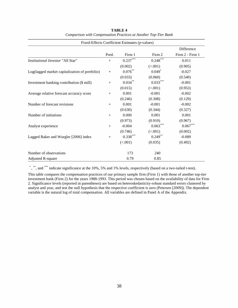
Compensation regressions for the primary and secondary firms (firms 1 and 2,

respectively) as well as statistical tests of differences are reported in Table 4 (for brevity, we

23 One firm, McLagan Partners, provided most of the benchmarking data and consulting services for financial services and

securities firms for much of our sample period.

29

report only the fixed-effects results). The similarity of results across the two banks increases our

confidence that the sample firm findings are not purely idiosyncratic.

7. Conclusion

Prior research has shown analysts at leading investment banks to have the ability to drive

security prices (e.g., Stickel [1995] and Womack [1996]), trading volume (e.g., Irvine [2000,

2004] and Juergens and Lindsey [2009]), and corporate financing activity (e.g., Krigman et al.

[2001]). Although much has been written about the explicit incentives of these important

information intermediaries, because prior hypotheses have not been subjected to direct empirical

testing, financial economists have been unable to make ceteris paribus statements regarding the

determinants of analysts’ compensation. This study, which uses nearly two decades of

compensation data from a large investment bank, is a first step towards closing this gap in the

literature.

Prior studies have argued that analysts face strong, bonus-based forecasting incentives.

This assumption is often motivated by associations between forecast accuracy and Institutional

Investor “All-Star” status, which are linked anecdotally to analyst compensation (e.g., Stickel

[1992]). Our paper challenges this view. Although All-Star status is strongly associated with

analyst pay, the variation in All-Star status that drives analyst pay is orthogonal to forecast

accuracy measured using a wide variety of forecast periods and estimation methods.

The compensation consequences of All-Star status cannot be attributed solely to All-Star

analysts having greater investment banking deal flow. Controlling for investment banking

contributions and a host of other variables, we find that II-ranked analysts earn 61% more than

non-II-ranked analysts. Fixed-effects regressions that control for unobserved analyst

heterogeneity show that gaining (losing) II status confers an immediate compensation premium

30

(penalty) equal to approximately 16% of annual compensation. Additional tests show analyst

compensation to be related to II votes even for analysts not mentioned in II magazine. II votes

are strongly related to buy-side client votes, which are used to allocate commissions across

banks. Together these relationships suggest that the II compensation effect likely represents

rewards for generating institutional trading commission revenues.

Not surprisingly, investment-banking contributions are an important determinant of

analyst remuneration. But only equity underwriting activities are associated with analyst pay. For

our sample firm, we find no evidence that sell-side equity analyst compensation is related to debt

or M&A underwriting. We find that larger equity underwriting deals are associated with larger

rewards, but there is no evidence that analysts are paid more for deals involving new (as opposed

to existing “relationship”) clients.

Our findings also indicate that analysts are rewarded for profitable stock

recommendations, but the effect is delayed and economically significant only if it generates

visibility in the WSJ’s annual stock-picking report. Recognition rather than underlying stock-

picking performance seems to account for much of the WSJ effect. Also, tests indicate that the

compensation rewards for superior recommendation performance are received in the period in

which the WSJ’s awards are announced, not the preceding year when then the superior

performance occurred.

Finally, analysts who cover large portfolios earn significantly more than analysts who

cover smaller portfolios. This factor appears to arise primarily from more talented analysts being

matched to economically important industries or stocks and receiving higher pay for their ability.

Given that annual compensation captures only a portion of total analyst incentives, we

examine the characteristics of analysts who likely were “fired” from our sample bank (i.e.,

31

moved to lower-status banks or brokerages, or exited I/B/E/S). Consistent with prior literature,

we find that “fired” analysts have large relative forecast errors in their final full year of

employment. This finding, taken in conjunction with the lack of association between

compensation and forecast accuracy, suggests that analysts’ forecasting incentives resemble a

Mirrlees contract. Under a normal range of forecast outcomes there is no relation between

forecast performance and compensation within banks, but extremely negative forecasting

outcomes are associated with increased probability of dismissal. This finding is important in light

of recent growth in the number of forecast-accuracy-based analyst turnover studies (e.g., Ke and

Yu [2006], Ertimur et al. [2008], Call et al. [2009], and Pandit et al. [2009]), as it suggests that

researchers are looking in the right place, but should be careful when generalizing their

inferences to discussions of analyst bonuses, as some have done.

Our findings suggest several avenues for future research. First, more research on client-

ratings seems warranted. For example, how are client ratings affected by the quality of analysts’

industry and firm analyses, ability to provide access to corporate managers, and responsiveness

to client questions? Similarly, what is the relation between client votes, brokerage-level trading

volume in covered stocks, and commission revenues? Second, given that the WSJ star premium

appears to, and the II star premium not to, reflect visibility in the media, future research on

incentives for analysts to generate public recognition and visibility also seems warranted.

Finally, future research could examine how the compensation practices at banks vary depending

on the sources of funding for research. For example, how are analysts compensated at brokerage

firms and lower-status banks at which investment-banking opportunities are less prevalent?

Similarly, how effective was the Global Settlement in limiting the degree to which compensation

is tied to banking deals?

32

FIGURE 1 Sell-side Analysts’ Total Compensation (in 2005 dollars)

This figure, based on a total of 609 analyst-year observations, plots total real compensation for all I/B/E/S-listed, U.S. sell-side analysts at a major financial institution

during the years 1988-2005. Total compensation equals salary plus bonus. Compensation data were inflation-adjusted using CPI data from the Federal Reserve

Economic Database (FRED).

33

FIGURE 2

Sell-side Analysts’ Salary and Bonus Compensation (in 2005 dollars)

This figure, based on a total of 609 analyst-year observations, plots real salary and bonus compensation for all I/B/E/S-listed, U.S. sell-side analysts at a major

financial institution during the years 1988-2005. Compensation data were inflation-adjusted using CPI data from the Federal Reserve Economic Database

(FRED). Median salary (bonus) is denoted by the dashed (solid) line. Vertical bars denote the inter-quartile range (i.e., first and third quartiles) of the salary and

bonus distributions.

34

FIGURE 3

Sell-side Analysts’ Compensation and Capital Market Activity

This figure plots the relation between mean sell-side analyst compensation and capital market activity. The sample consists of all I/B/E/S-listed, U.S. sell-side

analysts at a major financial institution during the years 1988-2005. Total compensation equals salary plus bonus. Compensation data were inflation-adjusted

using CPI data from the Federal Reserve Economic Database (FRED). Capital market activity is measured using the Baker and Wurgler [2006] index, which

captures a variety of capital market activity signals including banking-related variables (such as IPO volume, first day IPO returns, and equity share in new

issues) and commission-related variables (such as average monthly turnover on NYSE-listed stocks).

35

TABLE 1

The Determinants of Analyst Compensation

Coefficient estimates (p-values)

Model 1: Model 2: Model 3:

"Within Analyst" "Between

Analyst"

Pred. Pooled Fixed-Effects Cross-Sectional

Institutional Investor "All-Star" + 0.476 ***

0.145 ***

0.736 ***

(<.001) (0.003) (<.001) Log (lagged market capitalization of portfolio) + 0.178

*** 0.069

*** 0.185

***

(<.001) (0.012) (<.001) Investment banking contribution ($ mill) + 0.070

*** 0.058

*** 0.102

***

(<.001) (<.001) (<.001) WSJ star stock-picker + 0.209

*** 0.104

** 0.518

*

(0.009) (0.042) (0.059) Average relative forecast accuracy score + 0.001 0.000 -0.001

(0.654) (0.852) (0.806) Number of forecast revisions + 0.000 0.001 -0.002

(0.717) (0.288) (0.469) Number of initiations + -0.005 0.006 0.013

(0.610) (0.417) (0.575) Analyst experience + 0.000 0.019

** 0.007

(0.996) (0.038) (0.481) Lagged Baker and Wurgler [2006] index + 0.369

*** 0.310

*** 0.395

**

(<.001) (<.001) (0.028)

Number of observations 401 374 116

Adjusted R-square 0.45 0.83 0.53

* ,

**, and

*** indicate significance at the 10%, 5% and 1% levels, respectively (based on a two-tailed t-test).

This table reports compensation response coefficients for analysts employed by a high-status investment bank

during the years 1994-2005. Significance levels (reported in parentheses) are based on heteroskedasticity-robust

standard errors clustered by analyst and year, and test the null hypothesis that the respective coefficient is zero

(Petersen [2009]). Model 3 is based on the mean value of each variable across all years during which an analyst

was employed by the sample firm. Because this “between-analyst” cross-sectional model includes only one

observation per analyst, we report significance levels based on White’s [1980] heteroskedasticity-robust standard

errors. The dependent variable is the natural log of total compensation. All variables are defined in Panel A of

the Appendix.

36

TABLE 2 Comparing Alternate Measures of Earnings Forecast Performance: Standardized Pay-for-Accuracy Coefficients

Annual Metrics Quarterly Metrics

Panel A: Full Sample 1988-2005

Pred.

Standardized

Coefficient

Estimate p-value

Standardized

Coefficient

Estimate p-value

Absolute Accuracy:

-(Average undeflated absolute forecast error) + 0.006 0.812 -0.002 0.932

-(Average price-deflated forecast error) + 0.005 0.854 0.021 0.359

Relative Accuracy:

Average relative forecast accuracy score + 0.031 0.283 0.000 0.985

-(Average PMAFE) + 0.022 0.457 -0.004 0.870

-(Average PSAFE) + 0.029 0.307 -0.008 0.753

Panel B: WSJ EPS Sample 1994-2001

Pred.

Standardized Coefficient

Estimate p-value

WSJ star EPS forecaster + 0.046 0.681

* ,

**, and

*** indicate significance at the 10%, 5% and 1% levels, respectively (based on a two-tailed t-test).

Panel A reports standardized pay-for-accuracy coefficients for a variety of forecast accuracy indices commonly used in

the sell-side analyst literature. Each standardized pay-for-accuracy coefficient, β, is obtained by estimating the following

fixed-effect regression on the 1988-2005 sample (N = 567):

-1. ( ) ( . ) ( . )it i it t itStd ln Compensation Std Accuracy Index Std BakerWurgler

Std. ln(Compensation) is the natural logarithm of analyst compensation rescaled to have a mean of zero and standard

deviation of one. Std. Baker Wurgler is the Baker and Wurgler [2006] market activity index rescaled to have a mean of

zero and standard deviation of one. Std. Accuracy Index is the chosen forecast accuracy index averaged over all stocks

within analyst i’s portfolio in year t rescaled to have a mean of zero and standard deviation of one. To be included in the

annual metrics, an annual EPS forecast must be made between 90 and 360 days before the earnings announcement, and

the earnings announcement must occur within the compensation evaluation period. Each firm can contribute at most one

forecast to the annual accuracy metric. To be included in the quarterly metrics, a one-quarter ahead EPS forecast must be

made between 5 and 30 days before the quarterly earnings announcement, and the earnings announcement must occur

within the compensation evaluation period. Each firm can contribute, at most, four forecasts (one for each quarter) to the

quarterly accuracy metric. Additional details on the forecast accuracy indices are provided in the variable definition table

in Panel B of the Appendix.

Panel B reports the standardized pay-for-accuracy coefficient for an additional variable. WSJ star EPS forecaster is a

dummy variable that equals one if the analyst was named one of the “Best on the Street” earnings forecasters by the Wall

Street Journal in year t, and zero otherwise.

Significance levels are based on heteroskedasticity-robust standard errors clustered by analyst and year, and test the null

hypothesis that the respective coefficient is zero (Petersen [2009]).

37

TABLE 3 Comparing Alternate Measures of Stock-Picking Performance: Pay-for-Performance Coefficients

Fixed-Effect Coefficient Estimates (p-value)

Pred. Model 1 Model 2 Model 3 Model 4 Model 5

WSJ star stock-picker + 0.148 ***

0.134 **

(0.008) (0.015)

Average annualized return + 0.066 ***

0.050 **

(<.001) (0.049)

Market-adjusted BLT [2007] portfolio alpha + 0.053 ***

0.031

(0.001) (0.161)

Four-factor-adjusted BLT [2007] portfolio alpha + -0.008 -0.059 *

(0.803) (0.060)

Controlling for Baker and Wurgler [2006] index Yes Yes Yes Yes Yes

Controlling for other determinants No No No No No

Number of observations 339 339 339 339 339

Adjusted R-square 0.78 0.79 0.79 0.78 0.79

*

, **

, and ***

indicate significance at the 10%, 5% and 1% levels, respectively (based on a two-tailed t-test).

This table reports pay-for-stock-picking-performance sensitivities for analysts employed by a high-status investment bank during the years 1995-2005. This period

was chosen because I/B/E/S recommendation data became available in 1994, and to ensure consistency with the WSJ ratings, which are based on lagged stock-

picking performance. Significance levels (reported in parentheses) are based on heteroskedasticity-robust standard errors clustered by analyst and year, and test the

null hypothesis that the respective coefficient is zero (Petersen [2009]). The dependent variable is the natural log of total compensation expressed in real (2005-

equivalent) terms. The stock-picking performance indices are defined in Panel C of the Appendix.

38

38

TABLE 4

Comparison with Compensation Practices at Another Top-Tier Bank

Fixed-Effects Coefficient Estimates (p-values)

Difference

Pred. Firm 1 Firm 2 Firm 2 - Firm 1

Institutional Investor "All Star" + 0.237 ***

0.248 ***

0.011

(0.002) (<.001) (0.905) Log(lagged market capitalization of portfolio) + 0.076

** 0.049

* -0.027

(0.033) (0.060) (0.540) Investment banking contribution ($ mill) + 0.034

** 0.033

*** -0.001

(0.015) (<.001) (0.953) Average relative forecast accuracy score + 0.001 -0.001 -0.002

(0.246) (0.308) (0.129) Number of forecast revisions + 0.001 -0.001 -0.002

(0.630) (0.344) (0.327) Number of initiations + 0.000 0.001 0.001

(0.973) (0.910) (0.967) Analyst experience + -0.004 0.063

*** 0.067

***

(0.746) (<.001) (0.002) Lagged Baker and Wurgler [2006] index + 0.338

*** 0.249

** -0.089

(<.001) (0.035) (0.492)

Number of observations 173 240 Adjusted R-square 0.79 0.85

*

, **

, and ***

indicate significance at the 10%, 5% and 1% levels, respectively (based on a two-tailed t-test).

This table compares the compensation practices of our primary sample firm (Firm 1) with those of another top-tier

investment bank (Firm 2) for the years 1988-1993. This period was chosen based on the availability of data for Firm

2. Significance levels (reported in parentheses) are based on heteroskedasticity-robust standard errors clustered by

analyst and year, and test the null hypothesis that the respective coefficient is zero (Petersen [2009]). The dependent

variable is the natural log of total compensation. All variables are defined in Panel A of the Appendix.

39

39

REFERENCES

BARBER, B.; R. LEHAVY; AND B. TRUEMAN. “Comparing the stock recommendation

performance of investment banks and independent research firms.” Journal of Financial

Economics 85 (2007): 490–517.

BAKER, G. “Distortion and risk in optimal incentive contracts.” The Journal of Human

Resources 37 (2002): 728–51.

BAKER, G., AND B. JORGENSEN. “Volatility, noise and incentives.” Working paper, Harvard

Business School, 2003.

BAKER, M., AND J. WURGLER. “Investor sentiment and the cross-section of stock returns.”

Journal of Finance 61 (2006): 1645−80.

BANKER, R., AND S. DATAR. “Sensitivity, precision and linear aggregation of signals for

performance evaluation.” Journal of Accounting Research 27 (1989): 21–39.

BASU, S., AND S. MARKOV. “Loss function assumptions in rational expectations tests on

financial analysts’ earnings forecasts.” Journal of Accounting & Economics 38 (2004):

171–203.

BECKER, G. Human Capital: A theoretical analysis with special reference to education. New

York, NY: Columbia University Press for NBER, 1964.

BOLTON, P., AND M. DEWATRIPONT. Contract Theory. Cambridge, MA: The MIT Press,

2005.

BRADSHAW, M.; S. RICHARDSON; AND R. SLOAN. “The relation between corporate

financing activities, analysts’ forecasts and stock returns.” Journal of Accounting &

Economics 42 (2006): 53–85.

BRADSHAW, M. “Analysts’ forecasts: What do we know after decades of work?” Working

paper, Harvard Business School, 2008.

CALL, A.; S. CHEN; AND Y. TONG. “Are analysts’ earnings forecasts more accurate when

accompanied by cash flow forecasts?” Review of Accounting Studies 14 (2009): 358–91.

CAMERON, C., AND P. TRIVEDI. Microeconometrics: Methods and Applications. New York,

NY: Cambridge University Press, 2005.

CARTER, R.; F. DARK; AND A. SINGH. “Underwriter reputation, initial returns, and the long-

run performance of IPO stocks.” The Journal of Finance 53 (1998): 285–311.

CHRISTENSEN, P., AND G. FELTHAM. Economics of Accounting: Volume 2, Performance

Evaluation. New York, NY: Springer-Verlag, 2005.

40

40

CLARKE, J.; A. KHORANA; A. PATEL; AND P. R. RAU. “The impact of all-star analyst job

changes on their coverage choices and investment banking deal flow.” Journal of Financial

Economics 84 (2007): 713–37.

CLEMENT, M. “Analyst forecast accuracy: Do ability, resources, and portfolio complexity

matter?” Journal of Accounting & Economics 27 (1999): 285–303.

CLEMENT, M.; L. KOONCE; AND T. LOPEZ. “The roles of task-specific forecasting

experience and innate ability in understanding analyst forecasting performance.” Journal of

Accounting & Economics 44 (2007): 378–98.

COWEN, A.; B. GROYSBERG; AND P. HEALY. “Which types of analyst firms are more

optimistic?” Journal of Accounting & Economics 41 (2006): 119–46.

DUNBAR, C. “Factors affecting investment bank initial public offering market share.” Journal

of Financial Economics 55 (2000): 3–41.

EMERY, D., AND X. LI. “Are the Wall Street analyst rankings popularity contests?” Journal of

Financial and Quantitative Analysis 44 (2009) 411–37.

ERTIMUR, Y.; V. MUSLU; AND F. ZHANG. “The long-run performance of analyst coverage

initiations.” Working paper, Duke University, 2007.

ERTIMUR, Y.; B. MAYEW; AND S. STUBBEN. “Analyst reputation and the issuance of

disaggregated earnings forecasts to I/B/E/S.” Working paper, Duke University, 2008.

FRANCIS, J.; Q. CHEN; R. WILLIS; AND D. PHILBRICK. Security Analyst Independence.

Charlottesville, VA: The Research Foundation of CFA Institute, 2004.

FREDERICKSON, J.; S. PEFFER; AND J. PRATT. “Performance evaluation judgments: Effects

of prior experience under different performance evaluation schemes and feedback

frequencies.” Journal of Accounting Research 37 (1999): 151–65.

GASPARINO, C. Blood on the Street: The Sensational Inside Story of How Wall Street Analysts

Duped a Generation of Investors. New York, NY: Free Press, 2005.

GIBBONS, R., AND M. WALDMAN. “Careers in organizations: Theory and evidence,” in

Handbook of Labor Economics vol. 3, edited by O. Ashenfelter and D. Card. Amsterdam:

North-Holland, 1999: 2373–2437.

GREEN, T. C. “The value of client access to analyst recommendations.” Journal of Financial

and Quantitative Analysis 41 (2006): 1–24.

GREENE, W. Econometric Analysis. Englewood Cliffs, NJ: Prentice Hall, 2000.

41

41

GROYSBERG, B.; P. HEALY; AND C. CHAPMAN. “Do buy-side analysts out-perform the

sell-side?” Financial Analyst’s Journal 64 (2008): 25–39.

GU, Z., AND J. WU. “Earnings skewness and analyst forecast bias.” Journal of Accounting &

Economics 35 (2003): 5–29.

HINTZ, B.; M. WERNER; AND B. ST. JOHN. “U.S. securities industry: Institutional equities –

Searching for a new business model.” Bernstein Research, May 25, 2006.

HOLMSTRÖM, B. “Moral hazard and observability.” The Bell Journal of Economics 10 (1979):

74–91.

HOLMSTRÖM, B. “Managerial incentive problems: A dynamic perspective.” Review of

Economic Studies 66 (1999): 169–82.

HONG, H.; J. KUBIK; AND A. SOLOMON. “Security analysts’ career concerns and herding of

earnings forecasts.” The RAND Journal of Economics 31, 121–44.

HONG, H., AND J. KUBIK. “Analyzing the analysts: Career concerns and biased earnings

forecasts.” The Journal of Finance 58 (2003): 313–51.

IANNOTTA, G. Investment Banking: A Guide to Underwriting and Advisory Services. New

York, NY: Springer-Verlag, 2010.

INSTITUTIONAL INVESTOR. “The best analysts of the year.” Institutional Investor. October

1996.

INSTITUTIONAL INVESTOR. “The 1997 All-America research team.” Institutional Investor.

October 1997.

IRVINE, P. “Do analysts generate trade for their firms? Evidence from the Toronto Stock

Exchange.” Journal of Accounting & Economics 30 (2000): 209–26.

IRVINE, P. “Analysts’ forecasts and brokerage-firm trading.” The Accounting Review 79 (2004):

125–49.

JACKSON, A. “Trade generation, reputation, and sell-side analysts.” The Journal of Finance 60

(2005): 673–717.

JACOB, J.; T. LYS; AND M. NEALE. “Expertise in forecasting performance of security

analysts.” Journal of Accounting & Economics 28 (1999): 51–82.

JEGADEESH, N.; J. KIM; S. KRISCHE; AND C. LEE. “Analyzing the analysts: When do

recommendations add value?” The Journal of Finance 59 (2004): 1083–1124.

42

42

JUERGENS, J., AND L. LINDSEY. “Getting out early: An analysis of market making activity at

the recommending analyst’s firm.” Journal of Finance 64 (2009): 2327–59.

KE, B., AND Y. YU. “The effect of issuing biased earnings forecasts on analysts’ access to

management and survival.” Journal of Accounting Research 44 (2006): 965–99.

KRIGMAN, L.; W. SHAW; AND K. WOMACK. “Why do firms switch underwriters?” Journal

of Financial Economics 60 (2001): 245–84.

LEONE, A., AND J. WU. “What does it take to become a superstar? Evidence from Institutional

Investor rankings of financial analysts.” Working paper, University of Rochester, 2007.

MADAN, R.; R. SOBHANI; AND P. BHATIA. “Brokers & asset managers: Initiating coverage

– Higher lows were nice, but lower highs will be the price.” Citigroup/Smith Barney,

August 1, 2003.

MALLOY, C. “The geography of equity analysts.” The Journal of Finance 60 (2005): 719–55.

MAYER, T. “The distribution of ability and earnings.” The Review of Economics and Statistics

42 (1960): 189–95.

MCNICHOLS, M., AND P. O’BRIEN. “Self-selection and analyst coverage.” Journal of

Accounting Research 35 (1997): 167–99.

MERRILL LYNCH. “Research tops Journal’s ‘Best on the Street’ survey again.” May 2005.

http://www.ml.com/?id=7695_8134_8296_6018_46162_48002_48005.

MIKHAIL, M.; B. WALTHER; AND R. WILLIS. “Does forecast accuracy matter to security

analysts?” The Accounting Review 74 (1999): 185–200.

MIKHAIL, M.; B. WALTHER; AND R. WILLIS. “Does investor sentiment affect sell-side

analysts’ forecast accuracy?” Working paper, Northwestern University, 2009.

MILGROM, P., AND J. ROBERTS. Economics, Organization, and Management. Englewood

Cliffs, NJ: Prentice-Hall, 1992.

MURPHY, K. “Corporate performance and managerial remuneration: An empirical analysis.”

Journal of Accounting & Economics 7 (1985): 1–32.

O’BRIEN, P. “Forecast accuracy of individual analysts in nine industries.” Journal of

Accounting Research 28 (1990): 286–304.

O’BRIEN, P., AND R. BHUSHAN. “Analyst following and institutional ownership.” Journal of

Accounting Research 28 (1990): 55–76.

43

43

PANDIT, S; R. WILLIS; AND L. ZHOU. “Security analysts, cash flow forecasts, and turnover.”

Working paper, Vanderbilt University, June 2009.

PETERSEN, M. “Estimating standard errors in finance panel data sets: Comparing approaches.”

Review of Financial Studies 22 (2009): 435–80.

PRENDERGAST, C. “The provision of incentives in firms.” Journal of Economic Literature 37

(1999): 7–64.

PRENDERGAST, C. “The tenuous trade-off between risk and incentives.” The Journal of

Political Economy 110 (2002): 1071–1102.

RAITH, M. “Specific knowledge and performance measurement.” The RAND Journal of

Economics 39 (2008): 1059–79.

REINGOLD, D., AND J. REINGOLD. Confessions of a Wall Street Analyst: A true story of

inside information and corruption in the stock market. New York, NY: HarperCollins,

2006.

ROSEN, S. “Authority, control, and the distribution of earnings.” The Bell Journal of Economics

13 (1982): 311–23.

ROSEN, S. “Contracts and the market for executives,” in Contract Economics, edited by L.

Werin and H. Wijkander. Cambridge, MA: Blackwell, 1992: 181–211.

STICKEL, S. “Reputation and performance among security analysts.” The Journal of Finance 47

(1992): 1811–36.

STICKEL, S. “The anatomy of the performance of buy and sell recommendations.” Financial

Analysts Journal 51 (1995): 25–39.

VERBEEK, M. A Guide to Modern Econometrics. Hoboken, NJ: John Wiley and Sons, 2005.

WHITE, H. “A heteroskedasticity-consistent covariance matrix estimator and a direct test for

heteroskedasticity.” Econometrica 48 (1980): 817–38.

WOMACK, K. “Do brokerage analysts’ recommendations have investment value?” The Journal

of Finance 51 (1996): 137–67.

WOOLDRIDGE, J. Econometric Analysis of Cross Section and Panel Data. Cambridge, MA:

The MIT Press, 2002.

44

44

APPENDIX

Variable Definitions

For all variables, the subscript i refers to analyst i, the subscript j to stock j, and the subscript t to

year t, defined as the period from December 1, t-1, to November 30, t.

Panel A: Primary Variables

Variable Definition

Ln(Compensation)it Analyst i’s total compensation (salary + bonus) for year t,

expressed in real (2005-equivalent) dollars (sources: proprietary

compensation file, Federal Reserve Economic Database).

Institutional Investor “All-

Star”it

An indicator variable equal to one if analyst i was named an

“All-American” in the October year t issue of Institutional

Investor magazine, zero otherwise (source: Institutional

Investor).

Log(lagged market

capitalization of portfolio)it

For each of the j stocks in analyst i’s portfolio during year t we

measure the market capitalization on December 1, t-1 (i.e., at the

beginning of the performance evaluation period). We then sum

these amounts across the Jit securities in analyst i’s portfolio to

estimate the lagged aggregate market capitalization of analyst i’s

year t portfolio and take the natural logarithm (sources: CRSP,

I/B/E/S, Federal Reserve Economic Database).

Investment banking

contribution ($ mill)it

The estimated equity underwriting fees received by the sample

bank from all firms covered by analyst i in year t, expressed in

real (2005-equivalent) dollars. For deals in which the bank was a

book-runner, fees are estimated as

Management Fee

# of Book-runners+

Underwriting Fee + Selling Concession

# of Syndicate Members .

For deals in which the bank was not a book runner, fees are

estimated as Underwriting Fee + Selling Concession

# of Syndicate Members (sources:

SDC, I/B/E/S, Federal Reserve Economic Database).

WSJ star stock-pickerit An indicator variable equal to one if analyst i was named one of

the “Best on the Street” stock-pickers by the Wall Street Journal

in year t, and zero otherwise (source: the Wall Street Journal).

45

45

APPENDIX – Continued

Variable Definition

Average relative forecast

accuracy scoreit

The average accuracy of analyst i’s earnings forecasts in year t.

For each of the Jit firms covered by analyst i in year t we

compute relative accuracy using the following formula:

1100 100

ijt

jt

Rank

I

, where Ijt is the number of analysts

following firm j in year t and Rankijt is analyst i’s rank relative to

all other analysts covering firm j in year t based on absolute

forecast errors. See Figure A.1 for the timing and computation of

absolute forecast errors (source: I/B/E/S).

Number of forecast

revisionsit

The number of annual EPS forecasts issued between 90 and 360

days before the earnings announcement date (source: I/B/E/S).

Number of initiationsit The number of new firms covered by analyst i in year t.

Following McNichols and O’Brien [1997], we exclude

initiations issued within the first six months of an analyst’s

appearance in I/B/E/S (source: I/B/E/S).

Analyst experienceit The number of years that an analyst has appeared in I/B/E/S

(source: I/B/E/S).

Baker and Wurgler [2006]

indext-1

The lagged value of the Baker and Wurgler [2006] activity

index, which captures a variety of capital market activity signals

including banking related variables (such as IPO volume, first

day IPO returns, and equity share in new issues) and

commission-related variables (such as average monthly turnover

on NYSE-listed stocks) (source: Baker and Wurgler).

46

46

APPENDIX – Continued

Panel B: Additional Forecast Accuracy Variables (Table 2)

For all variables, Actualjt is the actual EPS announced by firm j during evaluation year t; for the

annual (quarterly) measures, Forecastijt is the last EPS forecast issued by analyst i for company j

between 90 and 360 days (5 and 30) before the announcement of Actualjt; Jit is the number of

stocks covered by analyst i during year t; Ijt is the number of analysts following stock j in year t;

and1

1 jtI

jt ijtjtijt

Actual Forecast Actual ForecastI

.

Variable Definition

Average undeflated

absolute forecast

errorit 1

1 itJ

jt ijt

jit

Actual ForecastJ

(source: I/B/E/S).

Average price-

deflated forecast

errorit 1 1

1 itJjt ijt

jit jt

Actual Forecast

J P

, where Pjt-1 is firm j’s stock price

measured at the beginning of the evaluation period (source: I/B/E/S,

CRSP).

Average DAFEit

1

1 itJ

jt ijt jtjit

Actual Forecast Actual ForecastJ

(source: I/B/E/S).

Average PMAFEit

1

1 itJjt ijt jt

jit jt

Actual Forecast Actual Forecast

J Actual Forecast

(source: I/B/E/S)

Average PSAFEit

1

1

.

itJjt ijt jt

jit jt

Actual Forecast Actual Forecast

J Std Dev Actual Forecast

(source: I/B/E/S)

47

47

APPENDIX – Continued

Panel C: Additional Stock-Picking Performance Variables (Table 3)

Variable Definition

Average

annualized

return i,t-1

The annualized return to buy and strong-buy recommendations computed

using the method employed by the sample bank (source: I/B/E/S, CRSP).

BLT1: Market-

adjusted BLT

[2007] portfolio

alphait-1

and

BLT2: Four-

factor-adjusted

BLT [2007]

portfolio alpha it-1

The long-window calendar-time “market-adjusted” and “four-factor-

adjusted” alpha obtained using the methodology in Barber, Lehavy, and

Trueman [2007].

To implement their approach, we create a portfolio of buy/strong-buy

recommendations and estimate daily returns to this portfolio using the

daily rebalancing technique described in BLT. We then estimate each

analyst’s abnormal stock picking performance for a given year as the

intercept, αit, from the following daily time-series regressions:

(BLT1) ( )d fd md fd d

it t it it t t itr r r r

(BLT2) ( )d fd md fd d d d d

it t it it t t it t it t it t itr r r r s SMB h HML w WML ,

where d

itr is the portfolio return on day d for analyst i in year t; fd

tr is the

CRSP daily risk-free return on day d in year t; md

tr is the daily return on the

CRSP value-weighted market index; d

tSMB is the return on day d in year t

of a value-weighted portfolio of small stocks minus the return on a value-

weighted portfolio of big stocks; d

tHML is the return on day d of year t of a

value-weighted portfolio of high book-to-market stocks minus the return

on a value-weighted portfolio of low book-to-market stocks; d

tWML is the return on day d of year t on a value-weighted portfolio of

stocks with high recent returns minus the return on a value-weighted

portfolio of stocks with low recent returns.

To facilitate comparability with the Average annualized return metric

employed by the sample bank, alphas are multiplied by 365 (source:

I/B/E/S, CRSP, Ken French’s website).