Computational Fluid Dynamics I Introduction to Computational Fluid Dynamics-I http://users.wpi.edu/~gretar/me612.html Grétar Tryggvason Spring 2010 Computational Fluid Dynamics I What is CFD A few examples Computational tools Short history Introduction Course goals Course content Schedule Homework and projects Textbooks on reserve Computational Fluid Dynamics I What is Computational Fluid Dynamics (CFD)? Computational Fluid Dynamics I Finite Difference or Finite Volume Grid Computational Fluid Dynamics I Grid must be sufficiently fine to resolve the flow Computational Fluid Dynamics I The number of grid points (or control volumes) available determines the complexity of the problem that can be solved and the accuracy of the solution
Transcript
Computational Fluid Dynamics I
Introduction to Computational Fluid
Dynamics-I!
http://users.wpi.edu/~gretar/me612.html!
Grétar Tryggvason!Spring 2010!
Computational Fluid Dynamics I
What is CFD!A few examples!Computational tools!Short history!
Introduction!Course goals!Course content!Schedule!Homework and projects!Textbooks on reserve!
Computational Fluid Dynamics I
What is Computational Fluid Dynamics (CFD)?!
Computational Fluid Dynamics I
Finite Difference or!Finite Volume Grid!
Computational Fluid Dynamics I
Grid must be sufficiently fine to resolve the flow!
Computational Fluid Dynamics I
The number of grid points (or control volumes) available determines the complexity of the problem that can be solved and the accuracy of the solution!
FLOPS (Floating-point operations per second)!CRAY-1 (1976) - 133 Megaflops!ASCI White (2000) - 12.28 Teraflops!
! Increase by a million in a quarter century !!!
Computational Fluid Dynamics I
CFD is used by many different people for many different things!
Industrial problems: The goal is generally to obtain data (quantitative and qualitative) that can be used in design of devices or processes. Often it is necessary to use “subgrid” or closure models for unresolved processes!Academic problems: The goal is to understand the physical aspects of the process, often the goal is to construct “subgrid” or closure models for industrial computations !
Computational Fluid Dynamics I
A few random examples!CFD is now a standard part of the toolkit used both in scientific studies and engineering predictions!
The numerical solution yields the velocity and pressure field everywhere. Usually, it is the force on a boundary that is of interest. Looking at the flow field can, however, be very informative!
Computational Fluid Dynamics I
Bubble Movie!
Computational Fluid Dynamics I Computational Fluid Dynamics I
Many website contain information about fluid dynamics and computational fluid dynamics specifically. Those include!
NASA site with CFD images!http://www.nas.nasa.gov/SC08/images.html!
CFD Online: An extensive collection of information but not always very informative!http://www.cfd-online.com/!
eFluids.com is a monitored site with a large number of fluid mechanics material!http://www.e-fluids.com/!
Computational Fluid Dynamics I
Short History of CFD!
http://users.wpi.edu/~gretar/me612.html!Computational Fluid Dynamics I
Richardson (1910)! Early vision of the role of numerical predictions
Courant, Friedrichs, and Lewy (1928)! Stability analysis of the advection equation (CFL condition) !
von Neumann! Role of computations, stability analysis !
Lax and the Courant group! Promoting numerical computations !
Harlow and the Los Alamos group! MAC, CIC, and other methods
Spalding and industrial applications! CHAM was the first provider of general-purpose CFD software. The original PHOENICS appeared in 1981.!
NCAR and the Supercomputer Centers!
Short history!
Computational Fluid Dynamics I
1963: J. E. Fromm and F. H. HarIow, Numerical Solution of!the Problem of Vortex Street Development: Phys. Fluids!6, 975. !
Computational Fluid Dynamics I
F. H. Harlow and J. E. Fromm, “Computer Experiments in Fluid Dynamics:ʼ Scientific American, Vol. 212, No. 3, 104 (1965).!
F. H. Harlow, J. P. Shannon, and J. E. Welch, “Liquid Waves by Computer” Science 149 (1965), 1092.!
D.B. Spalting, Int. J. Numer. Meth. Engr. 4 (1972), 1972!
Early papers about solutions of the Navier-Stokes equations!
Computational Fluid Dynamics I
Commercial Codes!
http://users.wpi.edu/~gretar/me612.html!Computational Fluid Dynamics I
CHAM (Concentration Heat And Momentum) founded in 1974 by Prof. Brian Spalding was the first provider of general-purpose CFD software. The original PHOENICS appeared in 1981.!
The first version of the FLUENT code was launched in October 1983 by Creare Inc. Fluent Inc. was established in 1988.!
STAR-CD's roots go back to the foundation of Computational Dynamics in 1987 by Prof. David Gosman,!
The original codes were relatively primitive, hard to use, and not very accurate.!
Short history!
Computational Fluid Dynamics I
What to expect and when to use commercial package:!
The current generation of CFD packages generally is capable of producing accurate solutions of simple flows. The codes are, however, designed to be able to handle very complex geometries and complex industrial problems. When used with care by a knowledgeable user CFD codes are an enormously valuable design tool. !
Commercial CFD codes are rarely useful for state-of-the-art research due to accuracy limitations, the limited access that the user has to the solution methodology, and the limited opportunities to change the code if needed !
Computational Fluid Dynamics I
Major current players include!
Ansys (Fluent and other codes)!! !http://www.fluent.com/ http://www.ansys.com/!
Computational Fluid Dynamics has traditionally been one of the most demanding computational application. It has therefore been the driver for the development of the most powerful computers!
What is CFD!A few examples!Computational tools!Short history!
Introduction!Course goals!Course content!Schedule!Homework and projects!Textbooks on reserve!
Computational Fluid Dynamics I
Prof. Gretar Tryggvason!Ph.D. Brown University 1985!Professor of Mechanical Engineering!University of Michigan ! ! ! ! 1985-2000!Professor and Head, Mechanical Engineering!Worcester Polytechnic Institute ! ! ! since 2000!Short term visiting/research positions: Courant, Caltech, !NASA Glen, University of Marseilles, University of Paris VI!Fellow of the American Physical Society and !the American Society of Mechanical Engineers!Associate Editor of the International Journal of Multiphase Flow !Editor-in-chief of the Journal of Computational Physics!
Instructor!
Computational Fluid Dynamics I
Coarse Goals:!Learn how to solve the Navier-Stokes and Euler equations for engineering problems using both customized codes and a commercial code!Hear about various concepts to allow continuing studies of the literature.!
Ways:!Detailed coverage of selected topics, such as: simple finite difference methods, accuracy, stability, etc.!Short introduction to FLUENT!Rapid coverage of other topics, such as: multigrid, monotone advection, unstructured grids.!
Computational Fluid Dynamics I
Preparing the data (preprocessing):!Setting up the problem, determining flow parameters and material data and generating a grid.!
Solving the problem!
Analyzing the results (postprocessing): Visualizing the data and estimating accuracy. Computing forces and other quantities of interest. !
Using CFD to solve a problem:!
Computational Fluid Dynamics I
Numerical !Analysis !
Fluid! Mechanics!
CFD!
Computer!Science!
CFD is an interdisciplinary topic!
Computational Fluid Dynamics I
Background needed:!
Undergraduate Numerical Analysis and Fluid Mechanics!
Graduate Level Fluid Mechanics (can be taken concurrently).!
Basic computer skills. We will use MATLAB for some of the homework.!
Computational Fluid Dynamics I
Part I!A brief introduction to CFD and !review of fluid mechanics !
Part II!Standard Numerical Analysis of partial differential equations !
Integrating a first-order ordinary differential equation in time!
dfdt
= g(t, f )
The initial condition must also be specified!
f (to ) = fo
Computational Fluid Dynamics I
dfdt
= g(t, f )
A numerical solution of!
consists of discrete values of f at discrete times!
f n = f (t) f n+1 = f ( t + Δt)
Δt Δt
f n−1 f n f n+1
Time!t − Δt t t + Δt
f n−1 = f ( t − Δt)
Time Integration!
f 1 = f (t0 + Δt) f 2 = f (t0 + 2Δt)f 0 = f (t0 )
�
f 0
�
t0
Computational Fluid Dynamics I
dfdt
= g(t, f )Start with!
rearrange!df = g(t, f )dt
�
dfn
n+1
∫ = g(τ, f )dτt
t+Δt
∫integrate!
�
f n+1 − f n = g(τ, f )dτt
t+Δt
∫
Time Integration!Computational Fluid Dynamics I
dfdt
= g( f ,t)
�
f n+1 = f n + g( f ,τ )dτt
t+Δt∫Integrate:!
Need to approximate!this area to evaluate!
the integral!
To advance: !
g
t t + Δt
gn gn+1 g( t)
Time Integration!
Computational Fluid Dynamics I
f n+1 = f n + gnΔt
g
t t + Δt
�
g( f ,τ )dτt
t+Δt∫ ≈ g(t)Δt = gnΔt
gn
Forward Euler!
Approximate:!
g( t)
Time Integration!Computational Fluid Dynamics I
f n+1 = f n + gn+1Δt
g
t t + Δt
�
g( f ,τ )dτt
t+Δt∫ ≈ g(t + Δt)Δt = gn+1Δt
gn+1
Backward Euler!
Approximate:!
g( t)
Time Integration!
Computational Fluid Dynamics I
f n+1 = f n + 12gn + gn+1( )Δt
g
t t + Δt
�
g( f ,τ )dτt
t+Δt∫ ≈ 12g(t) + g(t + Δt)( )Δt = 1
2gn + gn+1( )Δt
gn gn+1
Trapezoidal rule!
Approximate:!
g( t)
Time Integration!Computational Fluid Dynamics I
f n+1 = f n + gnΔt
f n+1 = f n + gn+1Δt
f n+1 = f n + 12gn + gn+1( )Δt
Forward Euler!
Backward Euler!
Trapezoidal Rule!
Summary:!
Time Integration!
Computational Fluid Dynamics I
Example!
Computational Fluid Dynamics I
g( f ,t) = − f
giving!dfdt
= − f
f t( ) = e−tthe exact solution is!
Accuracy!
Take!
If the initial condition is!
f (0) = 1
Computational Fluid Dynamics I
f n+1 = (1 − Δt) f n
f n+1 = f n
(1 + Δt)
f n+1 = (1 − Δt)(1 + Δt)
f n
f n+1 = f n − f nΔtForward Euler!
f n+1 = f n − f n+1ΔtBackward Euler!
f n+1 = f n − Δt2
f n + f n+1( )Trapezoidal Rule!
Accuracy!Computational Fluid Dynamics I A short code, using matlab (EX1)!
% a simple code for several integration methods!nstep=5;dt=0.5;!f1=zeros(nstep,1);f2=zeros(nstep,1); f3=zeros(nstep,1); !fex=zeros(nstep,1); t=zeros(nstep,1);!t(1)=0;f1(1)=1;f2(1)=1;f3(1)=1;fex(1)=1;!for i=2:nstep! f1(i)=f1(i-1)-dt*f1(i-1); %Forward Euler! f2(i)=f2(i-1)/(1.0+dt); %Backward Euler! f3(i)=f3(i-1)*(1.0-0.5*dt)/(1.0+0.5*dt); %Trapezoidal Rule! t(i)=t(i-1)+dt;! fex(i)=exp(-t(i));!end;!plot(t,f1);hold on;plot(t,f2,'r');plot(t,f3,'k');!plot(t,fex, 'r', 'linewidt',3); set(gca,'fontsize',24,'linewidt',2);!
Computational Fluid Dynamics I
0 0.5 1 1.5 20
0.2
0.4
0.6
0.8
1
Exact!
Forward Euler!
dfdt
= − f
Time!
ff = e−t
t=0.5!Backward Euler!
Trapezoidal rule!
Computational Fluid Dynamics I
Can we improve the accuracy of the forward and backward Euler method?!
Re-run the forward Euler method with smaller time steps!
Clearly the numerical solutions have the same behavior as the exact solution but only the trapezoidal rule results in numerical values that are approximately the same. The obvious question is:!
Computational Fluid Dynamics I
0 0.5 1 1.5 2 2.50
0.2
0.4
0.6
0.8
1
Exact!
Forward Euler!Method!
Time!
ff = e−t
t=0.5!
Accuracy, effect of t!
t=0.25!t=0.125!
Notice that the!results are!plotted versus!time, not time!step n!!
Computational Fluid Dynamics I
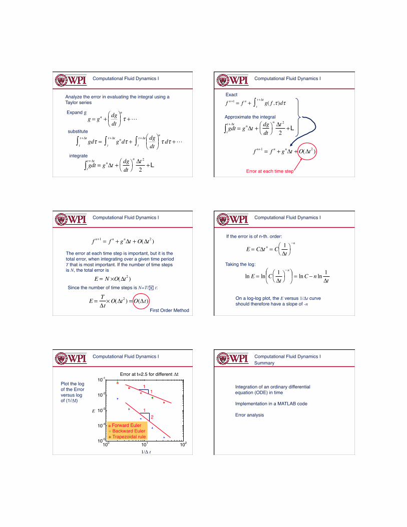
The error at t=2.5, for the forward Euler Method, defined by:!
As the time step becomes smaller, it is clear that the error goes to zero!
E
t
Forward Euler!+ Backward Euler! Trapezoidal rule!
E=| fnum(2.5)-exp(-2.5) |
Computational Fluid Dynamics I
Error Analysis!
Computational Fluid Dynamics I
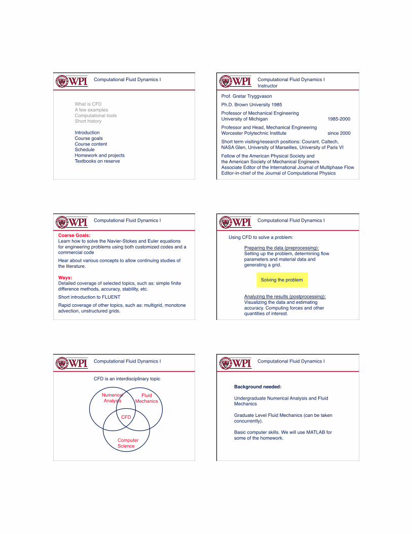
Analyze the error in evaluating the integral using a Taylor series!
�
g = gn + dgdt
⎛ ⎝ ⎜
⎞ ⎠ ⎟ n
τ +Expand g!
�
gdτt
t+Δt∫ = gndτt
t+Δt∫ + dgdt
⎛ ⎝ ⎜
⎞ ⎠ ⎟ n
τ dτt
t+Δt∫ +
substitute!
gdtt
t+ Δt
∫ = gnΔt +dgdt
⎛ ⎝
⎞ ⎠
n Δt 2
2+ L
integrate!
Computational Fluid Dynamics I
f n+1 = f n + gnΔt +O(Δt2 )
Error at each time step!
�
f n+1 = f n + g( f ,τ )dτt
t+Δt∫Exact !
gdtt
t+ Δt
∫ = gnΔt +dgdt
⎛ ⎝
⎞ ⎠
n Δt 2
2+ L
Approximate the integral!
Computational Fluid Dynamics I
E = N ×O(Δt2 )
f n+1 = f n + gnΔt +O(Δt2 )
The error at each time step is important, but it is the total error, when integrating over a given time period T that is most important. If the number of time steps is N, the total error is!
E =TΔt
×O(Δt2 ) =O(Δt)
Since the number of time steps is N=T/ t:!
First Order Method!
Computational Fluid Dynamics I
E = CΔt n = C 1Δt
⎛ ⎝
⎞ ⎠
−n
On a log-log plot, the E versus 1/Δt curve should therefore have a slope of -n!