What Makes Brain Drain More Likely?Measuring the Effects of Migration on the Schooling Investments

of Heterogeneous Households I

Romuald Meangoa,

aMax Planck Institute for Social Law and Social Policy,Amalienstr. 33, 80799, Munich, Germany

Abstract

This paper studies the effects of migration on the schooling investment of heteroge-

neous households. I use an IV-discrete choice model of schooling investment, which

distinguishes between migration attempts and actual migrations to (partially) iden-

tify the net effect of migration on schooling investments. Looking at emigration from

Senegal to Europe, I find a negative net effect of migration on the enrollment in up-

per secondary education for many sub-groups of households in Senegal. Interestingly,

there is a gender difference in the causes of these negative signs: positively skill-biased

migration leads to the negative net effect observed on women, whereas disincentives

to invest in education drive the negative net effect observed on men. Furthermore,

the analysis suggests that financially constrained households substitute an investment

in migration to an investment in education.

Keywords: Migration, brain drain, brain gain, sharp bounds.

JEL: C30, I25, J61.

IFinancial support by the Leibniz Association (SAW-2012-ifo-3) is gratefully acknowledged.Email address: meango@mea.mpisoc.mpg.de (Romuald Meango)

1. Introduction

Despite all its negative connotations, the term “Brain Drain” has come to dom-

inate the popular discourse about high-skilled migration. This dominance betrays

a perception of high-skilled migration as a permanent loss of human capital experi-

enced by the sending countries. Indeed, the disproportionately larger emigration of

the high-skilled, when compared to the low-skilled migration, is a well established fact

that should be primarily understood as a selection effect.1However and increasingly,

economists warn that one should not be over-pessimistic about the effects of migra-

tion on the resulting human capital of the sending country, especially of a developing

country. One reason is that migration prospects from some developing country A to

some developed country B might create non-negligible incentives for further human

capital accumulation in A. The resulting effect has been coined “brain gain” and

can be understood as an incentive effect. Then, from the perspective of the source

country A, what is important is the resulting net effect, rather than the sole selec-

tion effect. Indeed, if a sizable proportion of migration candidates stays in A after

upgrading education, or part of the educated migrants returns, A might benefit from

an increase in its overall human capital. One would then talk about a “positive net

effect” or a “net brain gain” for source country A.2

As developed countries compete more fiercely to attract foreign talents, govern-

ments of developing countries ponder what should be the appropriate policy response

to high-skilled migration. They expect from economists answers to at least three

essential questions: what makes “brain drain” more likely? Does “brain gain” exist?

what determines the sign and magnitude of the net effect?3 Probably because of an

understanding of the “brain drain” as a macroeconomic issue, the empirical microeco-

nomic literature has so far concentrated on establishing the existence of the incentive

effect4, leaving to the empirical macroeconomic literature the task to establish the

1In one of the largest existing dataset on bilateral international migration, Docquier and Marfouk

(2006) find that the emigration rate is five to ten times higher for individuals with more than twelve

years of than for workers with less than twelve years of education.2Beine, Docquier, and Rapoport (2001, 2008) also use the term beneficial brain drain.3The first and second question have been asked by Gibson and McKenzie (2011a).4Gibson and McKenzie (2011b) is an exception. They ask the first of the three questions, but

look at the issue only indirectly by exploring the determinants of high-skilled migration from small

2

determinants of this net effect.5

This paper takes a new approach to the empirical study of the effects of migration

on the source country’s human capital by differentiating the selection, incentive and

net effects at the household level. I study these effects for households in Dakar, the

capital city of Senegal, a Sub-Saharan African country with a large “brain drain”

rate. I argue that the differentiation at the household level is relevant in at least

three respects: (1) it helps understanding the microeconomic mechanisms leading

to the observed macroeconomic effects. The empirical analysis below clearly shows

that well-off families invest more in secondary education when there exist emigration

prospects, while other families might even disinvest in upper secondary education.

This and further results point to credit constraints that force poor families to sub-

stitute a migration investment to a schooling investment. Thus, the observed “brain

drain” is the result of a market imperfection and should be addressed with corrective

policies. (2) Related to this point, the focus on household helps designing targeted

interventions at well identified units. In the short and middle term, targeted inter-

ventions represent a more promising avenue to address concerns about the “brain

drain” than vast governmental policies to upturn structural trends. In the context

of Senegal, funding a skill-selective migration scheme for poor families could correct

the market imperfection, and induce more investment in education. (3) Finally, the

asymmetric distribution of incentives has in turn distributional effects. In a context

where the sign of the net effect depends on the economic status of the household, one

should question the implication of migration for social mobility in the next generation.

To measure the incentive and the net effect, one needs to compare the schooling in-

vestment in the observed (factual) state of the economy to the schooling investment in

an hypothetical (counterfactual) situation where migration rules are stricter. As the

main challenge is to retrieve the counterfactual schooling investment, a model describ-

ing investment in education in the presence (and absence) of an emigration option is

Pacific countries.5For example Beine, Docquier, and Rapoport (2001, 2008) shows that the brain drain is most

severe in countries with small population or with high migration rates. The net brain gain exists

mostly for countries combining initially low levels of human capital and low emigration rates. See

also Kapur and McHale (2005) and Docquier and Rapoport (2012) who provide excellent discussions

and surveys on the recent theoretical and macroeconomic literature on the brain gain hypothesis.

3

necessary. I introduce a simple discrete choice model in a human capital investment

framework where a household take two decisions for a child: one about education

and one about migration. These decisions are described as simultaneous, and both

depend on observed as well as unobserved characteristics correlated across decisions.

The “brain gain” hypothesis emphasizes that the realization of the migration project

is subject to some randomness and that some candidates to migration are forced to

stay in the home country. The model explicitly accounts for this discrepancy between

the migration decision and the actual migration, and uses it as an additional source of

identification. The proposed model improves on the previous literature in that it (i)

accounts explicitly for the migration perspectives, and (ii) allows quantifying different

net effects of the brain circulation for different household’s characteristics. Contrary

to other studies though, e.g. Batista, Lacuesta, and Vicente (2012), the identification

strategy imposes a focus on one precise counterfactual: the closed economy, where

no migration prospect exists. Nevertheless, this is a counterfactual largely discussed

in the literature, for example Mountford (1997), Stark, Helmenstein, and Prskawetz

(1997), and Beine, Docquier, and Rapoport (2001, 2008).

Point identification of the incentive and the net effect in this framework is chal-

lenging as it requires large exogenous variations to isolate the counterfactual schooling

investment. I argue that, given the data at hand, to entertain such assumptions on

the exogenous variations would be untenable. Nevertheless, the model delivers simple

tractable bounds on the counterfactual schooling investment. These bounds can be

used to test for the existence of strictly positive incentive effects, even without instru-

ment. When an instrument is available, the bounds require, neither the satisfaction

of a “large support” condition, nor a specification of an equation of the migration

decision. Moreover, the bounds are derived under mild exogeneity assumptions.

The empirical analysis of schooling investment in Senegal uses the MAFE (Mi-

gration form Africa to Europe Project) dataset, which contains detailed information

on migrants and non-migrants from Senegal. Most importantly, the data provides

information on attempts to migration, as well as detailed information on the respon-

dent’s network, which I use to construct some exclusion restrictions. I find that the

net effect is essentially negative in the population, meaning that the average school-

ing level in Senegal would have been higher in a closed economy. Only rich families

seem to invest more in education because of emigration prospects. Poorest families

4

seem to disinvest the most in upper secondary education, suggesting that borrowing

constraints are the causes of the disinvestment. Consistent with this explanation, in

families where one member lives abroad and is likely to send remittances, the school-

ing investment is less elastic to emigration prospects than it is in similar families

without a migrant member. Finally, there is almost no evidence of a net positive

effect, even after accounting for return migration.

The rest of paper proceeds as follows: Section 2 links the present paper to the

existing literature on the brain drain/brain gain topic. Section 3 motivates the mea-

sures for the net effect of the emigration prospects on human capital accumulation,

and introduces the discrete choice model that describes schooling decisions in the

presence of an emigration option. Subsequently, Section 4 discusses identification

issues and derives the bounds on the net effect. Section 5 describes the background

to education, migration and the brain drain in Senegal. Section6 presents the MAFE

dataset, along with some insightful descriptive statistics. Section?? presents the esti-

mation methodology. Then, Section 8 presents and discusses the estimation results,

and, finally, Section 9 concludes. Technical proofs are relegated in the Appendix.

2. Related Literature

The “brain drain” argument as exposed, for example by Bhagwati and Hamada

(1974), emphasizes the loss of human capital incurred by low-income countries due

to positive skill-biased emigration. This loss impedes growth by depriving developing

country from the output and positive externalities generated by high-skilled migrants.

The so-called “brain drain” should be understood as a selection effect, in that high

skill individuals select themselves more often into migration; thus they are overrep-

resented among migrants and underrepresented in the origin country. Against this

background, the seminal contributions from Mountford (1997) and Stark, Helmen-

stein, and Prskawetz (1997), among others, pioneered a more optimistic view on the

consequences of the high-skilled emigration, by pointing out the incentive effect of

emigration prospects on human capital acquisition. This insight has been confirmed

in several empirical studies, including Batista, Lacuesta, and Vicente (2012), Chand

and Clemens (2008), Shrestha (2015), Theoharides (2015). Nevertheless, other studies

also point out the possibility that in a context of low returns to education, emigration

prospects produce negative incentives. Girsberger (2014) finds that labor migration

5

from Burkina Faso to Cote d’Ivoire lowers the educational attainment in rural re-

gions of Burkina Faso. This labor migration is to work in Cocoa plantations, where

no formal education is required. McKenzie and Rapoport (2011) show that household

migration from US to Mexico can lower educational attainment of children, which the

authors attribute to low returns to education for illegal migrants in the United States.

At the empirical level, studies on the net effect of emigration prospects on human

capital formation at the individual level face the challenge to find plausible exogenous

variations on the emigration prospects. Chand and Clemens (2008) use a quasi-

experimental set-up after a military coup in Fiji, while Shrestha (2015) relies on a

quasi-experimental setting about enrollment in the British Army in Nepal. Overall,

the challenge remains the external validity of these specific experiments.

The framework of this paper is closest to the one of Batista, Lacuesta and Vicente

(2014) (henceforth BLV) who study the case of Cape Verde using an instrumental

variable strategy. They propose testing for the existence of the incentive effect by

testing for a significant linear correlation between the own future probability of mi-

gration and the schooling decisions. Using simulation methods, they then estimate

the country-wise net effect of the emigration prospects on the enrollment in upper

secondary schools. This study improves on their work in several respects. The unique

data used here allows observing migrants in their destination countries, while BLV

have the concern that households who emigrate and leave no one in the origin coun-

try are not accounted for.6 Moreover, the data contains information on migration

attempts by the respondents, which is unobserved by BLV, but allows testing for a

strictly positive incentive effect even without an instrument. The present study also

presents methodological advances. While BLV measure an average effect of emigra-

tion prospects on schooling incentives, the methodology used here quantifies different

effects for different individual’s characteristics. Moreover, I substantially relax their

stringent assumptions on the functional form of the model equations, the structure of

the error terms and the properties of the instrumental variables. Indeed, the model

proposed below uses very general functional forms. These functional forms would

reduce to BLV’s Simultaneous Equation Model only at the cost of high level assump-

tions about the linearity and additive separability in the parameters. Besides, I do

6This possible source of biases is studied by Steinmayr (2014).

6

not make any parametric assumption on the error terms. Moreover, the proposed

methodology is immune to weak instrument biases, which sometimes seems to be

problematic in BLV’s framework and with our data. Finally, the validity of the in-

strument rests on a weaker exogeneity condition. This weaker set of assumptions can

be entertained because the proposed methodology estimates precise features of the

model rather than the full model. As noted by Heckman and Vytlacil (2001), weaker

assumptions produce more reliable results, but at the same time, cannot generate the

complete array of policy counterfactuals from estimates of the full model. While BLV

estimate an average net effect for different levels of the emigration prospects, this

study focuses on heterogeneous effects from one counterfactual scenario, the closed

economy, a counterfactual largely discussed in the literature, for example Mount-

ford (1997), Stark, Helmenstein, and Prskawetz (1997), and Beine, Docquier, and

Rapoport (2001, 2008).

Finally, note that remittances and return migration are alternative channels through

which the sending country can experience an increase in its human capital (Gibson and

McKenzie, 2011a; Dinkelman and Mariotti, 2014; Theoharides, 2015). The present

framework can isolate the contribution of return migrants to the observed human

capital. The latter is considered in Section 8.2. Although the data do not permit to

observe remittances at the time of schooling investment, I discuss the effect of having

a family member living abroad in this period.

3. Measures of the Effects of Migration on Schooling Decision

The usual measure of the net effect of migration on schooling investment compares

the level of schooling in the observed (factual) state of the economy to the level

of schooling in an hypothetical (counterfactual) situation where migration rules are

stricter, as described in Section 3.1. This paper focuses on a counterfactual situation

where no migration is possible: the closed economy.7 Since the factual household’s

schooling decision is observed, the main challenge is to retrieve the counterfactual

schooling investment in the case of closed economy; hence, the need for the model

in Section 3.2 that describes schooling investment decisions in the presence (and

absence) of an emigration option.

7Section ?? makes clear why identification is more difficult under other counterfactual scenarios.

7

3.1. Empirical Measures of the Selection, Incentive and Net Effect at the household

level

Let a household (parents and child) be characterized by W , a set of observable

characteristics, D the schooling attainment of the child, and Y the migration status

of the child, with Y = 0 when the child has not emigrated. The interest of this paper

is in the difference between the expected schooling decision of stayers in the current

state economy and the expected schooling decision in a closed economy, as measured

by:

∆(W ) := E(D|Y = 0,W )− E(Dcf |W ) (1)

where Dcf is the counterfactual schooling decision. ∆(W ) measures the gain or the

loss in the expected schooling level of the subgroup of individuals with characteris-

tics W , between the current open economy and a counterfactual closed economy. If

∆(W ) > 0, there is a positive net effect for the subgroup W . Conversely, if ∆(W ) < 0,

there is a net negative effect. ∆ is the measure of the net effect in the theoretical

models discussed by Mountford (1997), Stark, Helmenstein, and Prskawetz (1997),

and Beine, Docquier, and Rapoport (2001, 2008), now defined at the household level.

Note the decomposition:

∆(W ) = (E(D|Y = 0,W )− E(D|W )) + (E(D|W )− E(Dcf |W )).

The net effect results from two effects: the first term is the selection effect ∆sel(W ) :=

E(D|Y = 0,W )−E(D|W ), which stems from the difference in the skill composition of

migrants and stayers. The second term is the incentive effect, ∆inc(W ) := E(D|W )−E(Dcf |W ), which stems from emigration prospects changing the choice of education

compared to the counterfactual scenario without migration. The brain gain literature

emphasizes the case where the incentive effect is positive, in which case we talk of the

“brain gain” effect in group W = w. However, as discussed previously, there exists

instances where emigration prospects give disincentives to obtain further education.

The proposed measures can be easily modified to account additionally for return

migration. Denoting by R the pool of never-migrants and returned migrants, I can

define:

∆r(W ) ≡ E(D|i ∈ R,W )− E(Dcf |W ) (2)

8

Note that if ∆r > 0 while ∆ < 0, this points out to the importance of return migration

in compensating for the ex ante loss in human capital.

Among the preceding quantities, E(Dcf |W ) is the key unobserved one, and the

main interest of the following model of schooling investment.

3.2. A Model of Schooling Investment in the Presence of an Emigration Option

3.2.1. Sketch the model

I consider a framework based on the human capital literature, where education is

considered as an investment in future earnings and employment for rationale agents

who seek to maximize their lifetime earnings Willis, Rosen, and Heckman (1979).

One can see the education decision as one made by benevolent parents in order to

maximize the net lifetime earnings of the child. With imperfect credit markets, some

families will be able to invest in optimal education, while some other will invest until

the liquidity constraint is binding. As in Rosenzweig (2008), the returns to education

depends on the location where the individual works, either home or abroad.

Formally, I consider two periods, two education levels and two locations: an origin

country and a possible destination country. In the first period, a household with a

child makes two decisions: which schooling level the child should attain, and whether

the child should attempt emigration to the destination country at some cost. School-

ing investments are made in the first period. However, investments in migration

attempts await the second period and their success is subject to some randomness.

This randomness reflects both policy barriers from the sending and the receiving coun-

tries, as well as unexpected shocks preventing emigration of the candidate. In the

second period, given the obtained education, emigration is attempted, if the house-

hold decided so in the first period. The uncertainty on migration is solved and only a

proportion of candidates actually migrate. The child enjoys the returns to education

according to his location in the second period.

In this environment, risk neutral households with a subjective assessment of the

success probability choose in the first period their investment in education in order

to maximize their expected net lifetime earnings. The simple but powerful insight of

the model is that the expected schooling level in the closed economy is the expected

schooling level when no household makes an attempt to emigrate. This result holds

even if one considers binding budget constraints for the migration investment.

9

3.2.2. Further Notations

More formally, consider a household i that makes two decisions: one about edu-

cation and one about migration. Denote by Wi the information set of a household i

when the household makes the schooling and migration decisions in the first period.

Wi regroups a set of observable characteristics of i (age, gender, family size, family

physical capital, etc.), say Wi, and a vector of latent variables ui, unobserved by the

researcher.8

Recall that Di denotes the schooling attainment decided for the child by the house-

hold. I will consider two levels, which will correspond in our baseline to obtaining

at least some upper secondary education, or not. Denote by Y ∗i , a binary variable

describing the household’s decision to attempt migration, and equals 1 if i’s decides

to migrate. Again, Yi is the child’s actual migration status observed in the second

period.

The household has a subjective probability, that migration takes place given an at-

tempt migration, say pdi ≡ P (Yi = 1|Wi, Di = d, Y ∗i = 1). This subjective probability

depends on the educational attainment chosen by i. Based on the substantial evi-

dence from the empirical literature, we expect migration to be positively skill biased,

that is more educated are more mobile, so that p0i < p1i.

The counterfactual scenario of interest in this paper is the case of closed economy,

that is there is zero emigration probability. Thus, the main interest is in the schooling

choice when there is no emigration prospect, Dcf ; that is, i chooses Dcf,i when pdi

is counterfactually set to equal 0, for all d and i. E(Dcf,i|Wi) is the conditional

expectation of this quantity.

Finally, I borrow notations from the potential outcome literature, denoting by

Di(0) the child’s schooling attainment when Y ∗i is counterfactually set to equal 0

and Di(1), the corresponding schooling attainment when Y ∗i is counterfactually set

to equal 1. The simple insight of the model is that EDi(0) := E(Di(0)|Wi) =

E(Dcf,i|Wi). Therefore, the appropriate object of interest is the schooling choice

in the case where Y ∗i is counterfactually set to equal 0, Di(0).9.

8Section 4.4 gives a more precise description of information set.9Note that, in general, EDi(1) is not the same as the expected schooling level when pdi is

counterfactually set to equal 1. That is because, in the absence of migration barriers, individuals

10

In the rest of the paper, I drop the subscript i to lighten the notation.

3.2.3. The Schooling Decision

Consider the schooling decision given a decision on migration. It is assumed that

the household chooses the schooling level that maximizes the child’s expected return

given the migration choice. Let Πyd(W,u) be the net return (gains net of the costs)

to education d in location y, y ∈ {0, 1}.

Following the literature on returns to education, for example Dahl (2002), I will

assume for simplicity that the observed and unobserved returns to education are

separable, that is:

Πyd(W,u) = Πy

d(W ) + uyd (3)

Πyd(W ) is the average net expected return to education d for a household with charac-

teristics W . uyd is a latent cost of education that I interpret as the unobserved ability

of the child to complete education d or a private consumption value of education d.

Given a migration decision Y ∗, the household chooses education D = 1 over

D = 0, if and only if the following expression is positive:

Π01(W ) − Π0

0(W ) + u01 − u0

0

+ p1Y∗(Π1

1(W )− Π01(W ))− p0Y

∗(Π10(W )− Π0

0(W )) (4)

+ p1Y∗(u1

1 − u01)− p0Y

∗(u10 − u0

0)

The first line of Equation 4 represents the private returns to education D = 1, in the

absence of emigration prospects. The second and third lines represent the additional

incentive created by the emigration prospects. The second line stems from the average

returns given characteristics W , while the third line stems from the latent returns.

Note that the unobserved part of the total returns differs when Y ∗ = 1 or Y ∗ = 0,

which is the reason why standard regression techniques will produce biased estimates.

The simple implication of Equation (4) is that the education decision in the case

of closed economy is the same as the individual choice in the case where the migration

decision, Y ∗, is counterfactually set to be equal to 0. This is because the return to

education is the same whether p1 = p0 = 0 or Y ∗ = 0. Therefore E(Dcf |W ) = ED(0).

might not exert their migration option (Katz and Rapoport, 2005)

11

3.2.4. Binding budget constraint

Since imperfect credit markets are a common feature of developing economies, it

is important to account for the possibility of a binding budget constraint. Two cases

are possible: (1) the budget constraint is binding for education irrespective of the

migration decision, or (2) the budget constraint is binding for education only when

the family decides to attempt migration. Equation (4) already accounts for the first

possibility. In the second case, the maximization problem of the household includes

an additional term, λ(W,u)Y ∗ < 0, that reflects the constraint on the family. That

is the family maximizes:

Π01(W ) − Π0

0(W ) + u01 − u0

0

+ p1Y∗(Π1

1(W )− Π01(W ))− p0Y

∗(Π10(W )− Π0

0(W )) (5)

+ p1Y∗(u1

1 − u01)− p0Y

∗(u10 − u0

0) + λ(W,u)Y ∗

λ(W,u) should increase with the wealth of the family, and be zero if the budget

constraint is not binding. Conversely, if no borrowing opportunity exists, λ(W,u) =

−∞, and migration prospects do not provide additional incentives to obtain education

1. In the case of a constrained maximization, E(Dcf |W ) = ED(0) if no one attempts

migration for p1 = p0 = 0. The latter will be true under three plausible conditions: (1)

individuals maximize there expected returns to migration, (2) any migration attempt

is costly, and (3) yields a positive return only in the case of a successful emigration

(Y = 1).

To sum up, ED(0) is the proper object to compare with the level of education in

the open economy. Section 4 discusses the identification of ED(0). In particular, while

point identification of this quantity is challenging, one can easily derive tractable and

informative bounds. Before turning to the identification of ED(0), it is instructive to

pay more attention to the effects of emigration prospects on schooling returns.

3.3. The Effect of Emigration Prospect on Schooling Choice

At the heart of the brain gain literature is the assumption that, in the context

of skilled migration from developing to developed countries, the prospect of future

emigration gives positive incentives to acquire education. Two interrelated reasons

are evoked in the literature: first, the migration probability of high skilled is larger

12

than the migration probability of low-skilled individuals, so that returns to educa-

tion abroad matters more to high-skilled. Second, the absolute returns to education

(mostly measured by earnings gap between high skilled and low-skilled) are substan-

tially higher in developed countries than in developing countries (BLV).

There are two major exceptions to this hypothesis that are highly relevant in the

case of migration from Senegal to Europe: first, the case of a binding budget con-

straint (Beine, Docquier, and Rapoport, 2008), second, the case of illegal migration or

migration to low-skilled occupations (McKenzie and Rapoport, 2011). As described

above, when the budget constraint is binding, migration prospects do not provide ad-

ditional incentives to obtain further education. Moreover, the family might substitute

the migration investment to the schooling investment: candidates to migration might

drop out of school earlier in order to enter the labor market, and accumulate capital

that they will invest in a migration investment. Hence, migration prospects might

provide disincentives for poor families to invest in education.

Illegal migration or migration to low-skilled occupations might also provide disin-

centives for education for two reasons: first, the success of an illegal migration attempt

(e.g. traveling through the sea) depends less on the individual schooling attainment

than on borders surveillance. Thus, in the case of illegal migration p0 = p1 = p.

Second, job prospects for illegal migrants (e.g. picking tomatoes in rural region in

Spain) are not likely to depend on education, so that Π11(X) − Π1

0(X) is close to

zero. Hence, for someone who attempts illegal migration, the returns to education

are approximately:

(1− p0)× (Π01(X)− Π0

0(X)) + u01 − u0

0 + p0((u11 − u1

0)− (u01 − u0

0)).

Since schooling is completed in the origin country, we might expect that the unob-

served costs of education do not differ much by location, that is the last term in the

above the equation is close to zero. Then, on average, the returns to education will

be reduced by a factor p0, compared to the returns in a closed economy.

To sum up, since absolute returns to education are larger in Europe than in

Senegal, and following BLV’s result in Cape Verde, a neighbor country of Senegal, we

expect to find positive incentive effects. Possible exception are the subgroups where

the budget constraint is binding, especially poor families, and the subgroups where

illegal migration is highly prevalent. Whether the incentive effect can compensate for

13

the selection effect depends on intensity of the latter in each group.

4. Identification

This section discusses the identification of the net effect ∆, in particular, the

identification of the conditional expectation ED(0). First, Section 4.1 discusses the

assumptions required for point identification of the counterfactual quantity, and show

that informative bounds can be derived with less demanding assumptions. Then,

Section 4.2 makes explicit the bounds on ED(0). Subsequently, the bounds on the

measures of the net effect are presented in Section 4.3. These bounds exploit several

exogenous variations that can be found using a proper decomposition of the house-

hold’s information set, as described in Section 4.4.

4.1. Point identification

The above model of schooling investment belongs to class of Generalized Roy

models in the terminology of Heckman and Vytlacil (2007). It can also be called en-

dogenous treatment model (migration is the treatment and schooling the outcome).

Both observed and latent returns to education depend on the chosen location (or cho-

sen treatment). The model is “incomplete” according to the terminology of Chesher

and Rosen (2012), since it does not describe the selection into emigration. Typically,

non-parametric point identification will be obtained at the cost of assuming the exis-

tence of exogenous variations, say Z, that affects the migration decision but not the

schooling choice, and have a very large support (identification at infinity).

Even if the model was “completed” to describe the migration decision, non-

parametric identification is still challenging for existing methods, for example the

Local Instrumental Variable (LIV) as proposed by Heckman and Vytlacil (2001). The

LIV would require (i) an approximation of the migration decision through a latent

index equation, (ii) a monotonicity condition on the effect of the instrument(s) and

(iii) a set of instruments with a sufficiently large support. As discussed in Appendix

A, I view this set of assumptions as untenable in the present framework.

Therefore, I turn to the partial identification approach, which rests on a less

disputable set of assumptions.

14

4.2. Bounds on ED(0)

The model delivers simple tractable bounds on the counterfactual educational

attainment. When an instrument is available, sharper bounds can be derived, which

require no support or monotonicity conditions on the instrument.

Suppose that W = (X, Z), with Z such that Z, such that D(0) is stochatiscally

independent from Z conditional on X. The first and most intuitive bounds on ED(0)

are the bounds derived by Manski (1993). It suffices to note that:

ED(0) = P (D(0) = 1, Y ∗ = 0|X) + P (D(0) = 1, Y ∗ = 1|X)

The second term is unobserved, but bounded between 0 and P (Y ∗ = 1|X), so that:

P (D(0) = 1, Y ∗ = 0|X) ≤ ED(0) ≤ 1− P (D(0) = 0, Y ∗ = 0|X).

The bounds can be tightened by noting that E(D(0)|X, Z) = E(D(0)|X). Hence:

supZ

P (D(0) = 1, Y ∗ = 0|X, Z) ≤ ED(0) ≤ infZ

(1− P (D(0) = 0, Y ∗ = 0|X, Z)

).

The exogeneity condition on Z is a weaker condition than the one required by BLV

that require the existence of some Z, such that the pair (D(0), D(1)) is stochastically

independent from Z, conditionally on X. This additional condition produces tighter

bounds on the quantity ED(0), as given by the following proposition.

Proposition 1. All the following probabilities are conditional on X. Assume thatD(0) is stochastically independent from Z, conditionally on X, and the followingexpressions are well defined.

˜q10 := sup{ P(D = 1, Y ∗ = 0|Z = z) : z ∈ Supp(Z)}˜q00 := sup{ P(D = 0, Y ∗ = 0|Z = z) : z ∈ Supp(Z)}

the following are sharp bounds for ED(0).

˜q10 ≤ ED(0) ≤ 1− ˜q00

If in addition Z is such that (D(0), D(1)) is stochastically independent from Z,conditionally on X, and the following expressions are well defined:

q1 := inf{ P(D = 1|Z = z) : z ∈ Supp(Z)}q0 := inf{ P(D = 0|Z = z) : z ∈ Supp(Z)}q10−01 := inf{ P(D = 1, Y ∗ = 0|Z = z) + P(D = 0, Y ∗ = 1|Z = z) : z ∈ Supp(Z)}q00−11 := inf{ P(D = 0, Y ∗ = 0|Z = z) + P(D = 1, Y ∗ = 1|Z = z) : z ∈ Supp(Z)},q10 := sup{ P(D = 1, Y ∗ = 0|Z = z) : z ∈ Supp(Z)}q00 := sup{ P(D = 0, Y ∗ = 0|Z = z) : z ∈ Supp(Z)}

15

the following are sharp bounds for ED(0).

max(˜q10, 1− q0 − q00−11) ≤ ED(0) ≤ min(1− ˜q00, q1 + q10−01)

The tighter set of bounds follow by Corollary 2 of Mourifie, Henry, and Meango

(2015).

4.3. Bounds on the Net Effects

From bounds derived in the previous subsection, bounds for the measures ∆(.)

and ∆inc(.) follow trivially. Call LB0(X) (resp. UB0(X)) the lower (resp. upper)

bound derived in either Proposition 1, or 2, where the dependence on X is empha-

sized to remind the reader that the bounds vary with the individual characteristics.

The following bounds measure the net effect of brain circulation on human capital

accumulation in the source country :

E(D|Y = 0, X)− UB0(X) ≤ ∆(X) ≤ E(D|Y = 0, X)− LB0(X)

and accordingly for the measures ∆inc, ∆r and ∆rinc. Note that the selection effect

∆sel and ∆rsel are (point) identified.

An upper bound give the maximal magnitude of the corresponding net effect

(or maximal gain) possible in the sub-population of interest, while a lower bound

measures the minimal magnitude of the corresponding net effect (or maximal drain)

possible. If for ∆ the lower (resp. upper) bound is positive (resp. negative), there is

unambiguous evidence for a positive (resp. negative) net effect of migration on the

human capital accumulation with respect to the sub-population with characteristics

X = x. I will talk of a net brain gain (resp. net brain drain) in in the subgroup

x. If the upper bound is positive, while the lower bound is negative, the measure

is inconclusive about the direction of the effect. An optimistic interpretation will

focus on the upper bound, a pessimistic one on the lower bound. The same type of

interpretation pertains with respect to the measures ∆inc, ∆r and ∆rinc.

In Appendix B, I show that there exists additional non-redundant constraints on

the net effect ∆ that are described by Equation (6). ∆ must satisfy:

∆ ≤ P (D = 1, Y ∗ = 0) [1/P (Y = 0)− 1] + P (D = 1, Y ∗ = 1, Y = 0)/P (Y = 0)

∆ ≥ P (D = 1, Y ∗ = 0) [1/P (Y = 0)− 1] + P (D = 1, Y ∗ = 1, Y = 0)/P (Y = 0)

−P (Y ∗ = 1)

(6)

16

While the upper bound is almost surely larger that 0, the lower bound can take

either a positive or a negative sign. Thus, on can test for the existence of a strictly

positive net effect, even without an instrument.

4.4. The Information Set

The bounds in Proposition 1 exploit exogenous variations that can be found using a

proper decomposition of the household’s information set, as described in the following.

Recall thatW is the information set of a household when this household makes the

schooling and migration decisions in the first period. W regroups a set of observable

characteristics W , and a vector of latent variables u, unobserved by the researcher.

W can be further decomposed in the following:

1. X, the characteristics of the family and of the candidate that influence the

schooling choice both when no attempt is made, D(0), and when an attempt is

made, D(1), as well as the migration probability. These are for example, the

candidate’s age, gender, the family physical capital, the size of the family, etc.

2. X0, the characteristics that influence the returns to education at origin but not

at destination. These are for example, the macro-economic conditions in the

origin country.

3. X1, the characteristics that influence the returns to education at destination

but not at origin, for example, the labor market demand in the destination

country. For example, Theoharides (2015) takes advantage of the fluctuations

in the labor market demand in the destination countries, to identify the effect

of international emigration on the human capital of children in Philippines.

4. Z, the characteristics that influence the migration decision but not the schooling

decision irrespective of the decision to attempt migration. Z is a the type of

exclusion restriction assumed by BLV.

5. Z(1), the characteristics that affect the emigration prospects but do not affect

directly the choice of education when no attempt to migration is made. These

are for example, characteristics of the household facilitating visa approval, as

the existence of a sponsor.

From this decomposition of the information set, the net return to education can thus

17

be written:

Π01 (X,X0) − Π0

0 (X,X0) + u01 − u0

0

+ p1(X,X0, X1, Z(1))Y∗ (Π1

1 (X,X1)− Π01 (X,X0)

)(7)

− p0(X,X0, X1, Z(1))Y∗ (Π1

0 (X,X1)− Π00 (X,X0)

)+ p1(X,X0, X1, Z(1))Y

∗(u11 − u0

1)− p0(X,X0, X1, Z(1))Y∗(u1

0 − u00)

where the notation pd(X,X0, X1, Z(1)) emphasizes the role of these variables on the

success probability. From Equation (7), it follows that:

E(D(0)|W ) = E(D(0)|X,X(0)) (8)

Therefore, Z,X(1) and Z(1) can be used as exogenous variations to (partially) identify

ED(0). Note that for convenience of notation, I will use a slight abuse of notation

and refer to the vector X to denote the pair (X,X(0)).

I now turn to the empirical analysis on Senegal.

5. Background: Education, Migration and the Brain Drain in Senegal

5.1. Education

Between 1960, year of the independence from France, and 1990, the enrollment

rate in Senegal has steadily increased from 22 to 57% in primary school, and 2 to 16%

in Secondary school. The Senegalese educational system is modeled on the French

precedent. The typical curriculum consists of 6 years in primary school and 4 years

in lower secondary school, 3 years in upper secondary. At the end of each level, State

exams operate an increasingly selective screening of pupils, which outcome is often

based on available governmental resources. The “brain drain” question is all the

more relevant because the government devotes a large share of the total government

expenditures to education (between 16 to 22% in the past decade, that is 4 to 6%

of the GDP). Only recently, in 2004, have tuition fees for primary education been

abrogated and compulsory education introduced for children aged between 6 to 16

years10. At the time of the survey (2008), the enrollment rate was estimated at 84%

10Journal Officiel N 6202 du Samedi 22 Janvier 2005

18

in primary, 30% in Secondary, 8% in Tertiary. While the ratio male to female is the

same in primary school, it falls to 7 girls for ten boys in secondary.

Despite the importance of the public resources allocated to education and the

quantitative expansion in the enrollment rate, the performance of the educational

system is still weak (Niang, The primary school in Senegal: Education for all, quality

for some, 2014). Only one adult out of 2 is literate. As of 2013, Senegal ranks in

the last decile of the UNDP education index (which consists almost exclusively of

Sub-Saharan African countries, along with Afghanistan and Myanmar).11

5.2. Migration

Migration from Senegal has Africa and Europe as major destinations. Emigration

to Europe has a long tradition, which finds its roots in colonial ties with France.

Following the decolonization, a first wave of labor migration was sparked by an active

recruitment in French automobile industry. However, new immigration regulations

following the oil crisis in the mid 70’s provoked an abrupt closure of this migration

route Robin (1996), while introducing family reunification schemes. During the late

70’s until the mid 80’s, a new migration wave started as the result of poor economic

performances and repeated environmental shocks (droughts). However, with France

becoming increasingly less hospitable in comparison to other European coutries, mi-

grants from Senegal started to look for other destinations.12 This coincided with

increasing demands from the agriculture sectors in Spain and Italy Lacomba and

Moncusı (2006). During the late 80’s until the mid 90’s, further economic difficulties

in Senegal and in many Sub-Saharan countries, led to drastic cuts in public expendi-

tures. Rising unemployment and poverty, accompanied by a reduction in the provision

of public services acted as important push factors. Italy became all the more attrac-

tive as the demand grew for work in tourism and industry in northern Italy Obucina

(2013). Finally, in 1994, the long-lasting economic crisis, culminated in a devaluation

11The calculation of the UNDP education index accounts for the the mean years of schooling and

the expected years of schooling.12France introduced the requirement for a Visa for Senegalese workers, and launched initiatives

to encourage voluntarily repatriation of Senegalese workers, offering them paid formation in Sene-

gal. Source: Senegalese Embassy: http://www.ambasseneparis.com/index.php/cooperation.html,

accesed on Dec, 4, 2015.

19

of 50% of the Franc CFA. However, this measure did not have the expected effects

on the economy, and instead led to a deterioration of living conditions in the mid-

term. The devaluation also had the effect of doubling overnight the cost of (legal)

migration, as an importation good. This and increased immigration restrictions made

illegal migration more attractive and sophisticated. Half of 30,000 migrants who ar-

rived to Canary Island in 2006 where from Senegal Mbaye (2014). Meanwhile, the

high demand in the construction sector in Spain at the turn of the century continued

to fuel emigration flows (Baizan, Beauchemin, and Gonzalez-Ferrer, 2013).

5.3. Fear of “Brain Drain” in Senegal

Raw measures of the brain drain suggest that Senegal, as many countries in Sub-

saharan Africa, is highly affected by the self-selection of high skilled in emigration.

Although emigration is relatively low (as of 2005, a stock of 4.26% of the population,

with close to 40% of migrants in Europe) in comparison with countries with small

populations, the equally low level of high-skilled individuals and the strong discrep-

ancy between skilled and unskilled migration are the main stated concerns Easterly

and Nyarko (2008). According to Docquier and Marfouk (2006), in 2000, 17.7% of

the population with a tertiary education as emigrated. Baizan, Beauchemin, and

Gonzalez-Ferrer (2013) reports that 31% of migrants have some secondary educa-

tion, while only 16% in the remaining population. According to Beine, Docquier,

and Rapoport (2008)’s measure, when one accounts for the net effect of emigration

prospects, the computation of the net effect of emigration implies a loss of 0.2% of

the tertiary educated.

6. Data

6.1. MAFE Dataset

The empirical analysis is based on the longitudinal biographical survey data

collected in the framework of the MAFE (Migration between Africa and Europe)

Project.13 About 600 current Senegalese migrants in France, Italy and Spain and

13The MAFE project is coordinated by INED (C. Beauchemin) and is formed, additionally by the

Universit catholique de Louvain (B. Schoumaker), Maastricht University (V. Mazzucato), the Univer-

20

nearly 1100 residents of the region of Dakar were interviewed in 2008. As respondents

are sampled non-randomly, sampling weights are provided to produce a representative

sample.14 The survey collects retrospective biographical information about the demo-

graphic and socio-economic characteristics, labor force participation and migration of

the respondents and their household. There is additional information about migrant

networks, documentation status, remittances and asset ownership. A major attrac-

tiveness of the MAFE Dataset for this study is that it records the actual migration

history, as well as (unsuccessful) migration attempts, including year and destination

of attempt, and reasons of failure.

In the following analysis, I restrict the sample to individuals who never migrated

to Europe before the age of 21 to ensure that they obtained education in Senegal.

I also exclude individuals aged 60 or more who are part of the first migration wave

from Senegal and are underrepresented. This sample consists of 1342 individuals (626

men and 716 women).

6.2. Descriptive statistics

The data reveals an important gender difference in migration behavior, with the

female migrant population estimated between 19% to 29% of the migrant population.

Figure 1 shows both the proportion of the population who attempted migration to

Europe and the proportion of those who have been successful, by gender and educa-

tion level. Education is categorized in four groups: at most some primary education

(including those without education), some lower secondary education, some upper

secondary education, and some tertiary education. More educated individuals are

more likely to attempt migration, especially women, where the proportion of migra-

site Cheikh Anta Diop (P. Sakho), the Universit de Kinshasa (J. Mangalu), the University of Ghana

(P. Quartey), the Universitat Pompeu Fabra (P. Baizan), the Consejo Superior de Investigaciones

Cientficas (A. Gonzlez-Ferrer), the Forum Internazionale ed Europeo di Ricerche sull’Immigrazione

(E. Castagnone), and the University of Sussex (R. Black). The MAFE project received funding from

the European Community’s Seventh Framework Programme under grant agreement 217206. The

MAFE-Senegal survey was conducted with the financial support of INED, the Agence Nationale de

la Recherche (France), the Region Ile de France and the FSP programme ‘International Migrations,

territorial reorganizations and development of the countries of the South’. For more details, see:

http://www.mafeproject.com/14For more details on the MAFE project methodology, see Beauchemin (2012).

21

tion attempts nearly triples from primary to upper secondary education. The ratio

of success also varies substantially by education level. Where one out of two low

educated are successful in their attempt, at least two out of three high educated are

successful in their attempt. Note that on average an individual makes 1.35 (s.e.=0.06)

attempts to migrate, and the number of attempts increases with the education level:

from 1.27 (0.08) to 1.61 (0.17). Reassuringly, the Docquier and Marfouk (2006)’s es-

timate for the migration rate of tertiary educated (17.7%) belongs to the confidence

region as calculated on the sample.

Figure 3 compares the age at the first migration attempt for migrants and non-

migrants. Migrants make their first attempt much earlier than non-migrants. The

latter group consists of two main subgroups: those who attempt their first migration

around the age of 25, and later movers, who attempt migration after the age of 30.

This clearly suggests a selection that might depend on private information.

Figures 4 and 5 shows the distribution of the age at migration by gender and

education group respectively. The peak of the migration is attained around age 25.

Then migration rates decrease progressively to be almost nonexistent around age 40.

Women migrate later than men, suggesting tied-moving. The age at migration is

negatively correlated with the educational attainment, as the higher the education,

the earlier the migration. This is partly because of student migrants, but also because

the probability of success of a migration attempt decreases with the level of education.

Figures 6 shows the educational attainment by gender, migration status and co-

hort. The figures distinguish migrants to Europe from the rest of the population and

differentiate between three cohorts: individuals aged 25 to 34, 35 to 44 and 45 to 59.

Men are in general more educated than women. However, this gender gap seems to

have narrowed over the years, as more women are likely to obtain intermediary or

high education. This results from both the general expansion of education and the

recent public initiatives to promote gender equality in education. With regard to the

skill bias in migration, migrants to Europe are in general more educated than the

rest of the population. In particular, a larger proportion of migrants have obtained

at least some secondary education. But the distribution of educational attainment

varies across cohort, with an increasing selection on women, and an increasing, then

decreasing selection among men. This might be the result of the expansion in illegal

emigration, which has been more attractive to uneducated males in the recent years.

22

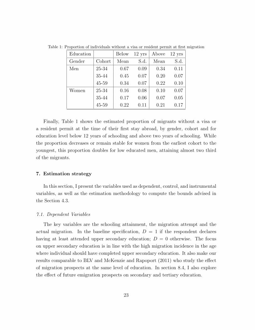
Table 1: Proportion of individuals without a visa or resident permit at first migration

Education Below 12 yrs Above 12 yrs

Gender Cohort Mean S.d. Mean S.d.

Men 25-34 0.67 0.09 0.34 0.11

35-44 0.45 0.07 0.20 0.07

45-59 0.34 0.07 0.22 0.10

Women 25-34 0.16 0.08 0.10 0.07

35-44 0.17 0.06 0.07 0.05

45-59 0.22 0.11 0.21 0.17

Finally, Table 1 shows the estimated proportion of migrants without a visa or

a resident permit at the time of their first stay abroad, by gender, cohort and for

education level below 12 years of schooling and above two years of schooling. While

the proportion decreases or remain stable for women from the earliest cohort to the

youngest, this proportion doubles for low educated men, attaining almost two third

of the migrants.

7. Estimation strategy

In this section, I present the variables used as dependent, control, and instrumental

variables, as well as the estimation methodology to compute the bounds advised in

the Section 4.3.

7.1. Dependent Variables

The key variables are the schooling attainment, the migration attempt and the

actual migration. In the baseline specification, D = 1 if the respondent declares

having at least attended upper secondary education; D = 0 otherwise. The focus

on upper secondary education is in line with the high migration incidence in the age

where individual should have completed upper secondary education. It also make our

results comparable to BLV and McKenzie and Rapoport (2011) who study the effect

of migration prospects at the same level of education. In section 8.4, I also explore

the effect of future emigration prospects on secondary and tertiary education.

23

The variable Y ∗ equals 1 if the respondent declares having attempted at least once

migration to Europe. Note that the survey provides information about all migration

attempts in all potential destinations as declared by the respondent.

Finally, since the dataset covers only the major destinations countries, Y , the

actual migration is observed (equals 1 when migration, 0 otherwise) for migrants to

these major destinations. To fit the definition of Y , ideally, we would like to sample

migrants in all European destination countries. This is a limitation of the present

data. The results presented here will hold, if migrants to other European destinations

are not too different from those present in the sample.

7.2. Heterogeneous Household Characteristics

The estimation strategy allows measuring heterogeneous net effects in the pop-

ulation. The empirical analysis addresses the heterogeneity with respect to gender,

cohort, and family background. Estimation of the bounds is conducted for men and

women separately. The measured effects are also differentiated for three cohorts: in-

dividuals aged 25 to 34, 35 to 44 and 45 to 59. The cohort 45 to 59 would correspond

to the second wave of migration between the 70’s and the mid 80’s, characterized

by the new labor migration to agriculture in Italy and Spain. The cohort 35 to

44 corresponds to the next wave of migration, between the mid 80’s and the mid

90’s, during the financial crisis and economic downturn in West Africa. This cohort

should be the one where liquidity constraints are the strongest. Finally the cohort

25 to 34 corresponds to the last wave of migration, characterized mainly by the high

attractiveness of illegal migration (see Section 5). With respect to family character-

istics, the estimation procedure controls for the occupation of the father when the

individual is 15.15 I construct four categories: High-level occupation or employer,

skilled employee, unskilled employee, and self-employed or unemployed. The effect of

parental occupation on the measured effects is of particular interest, since it allows

understanding whether poor or rich families are most likely to experience selection

or incentives. In line with the literature on household schooling choice, I also control

for the family size through a set of dichotomous variables that reflect the possibility

of a quality-quantity trade-off .

15Father’s education is also available but highly correlated to occupation.

24

To remain parsimonious, I assume that the effect of economic conditions in the

origin country is absorbed by the cohort dummies. Later on, I also control for the

religion (Mouride, Tidiane or others) and ethnicity (Pular, Wolof or others) that

capture potential migration networks.

7.3. Instruments

The first instrument follows from BLV’s insight that the longest migration spell

in the family at age 15 provides exogenous variation affecting the migration decision

but not the educational attainment at home. As noted by BLV, maximum length

of the family migration spell delivers information regarding the success of the closest

migration experience to the individual. Longer migration spells in the family reflect

more successful migration experiences that should translate into deeper access to

migrant networks.16

A second source of exogenous variation comes from characteristics affecting the

subjective probability of success but not the education decision. I use the number

of individuals known by the respondents between 16 and 21 and that migrate in this

period where upper secondary education should be completed. The rationale is that

individuals who observe more migration in their network, will be more optimistic

about their own chance of migration.

Because individuals with a stronger network would benefit from remittances and

savings that can be invested in education, one should ideally control for remittances

received by the family. As Beine, Docquier, and Rapoport (2008) argue, once one

controls for remittances, there is no obvious reason why migration network would

affect human capital formation. However, the MAFE dataset does not contain infor-

mation on the size of remittances at the age of 15. Controlling for parents’ occupation

partially address this concern. Following BLV, I control additionally for at least one

of the family member living abroad when the individual is aged 15 (around 20% of

the sample). Note that this concern would not affect the second instrument.

Finally, to take advantage of exogenous variations that affect the returns to edu-

cation abroad but not at home, I construct an index measure, which interacts, at a

16The second instrument in BLV, regional proportion of migrants, cannot be fruitfully used in our

context because the data are for individuals in the same geographical area.

25

given age, the strength of an individual’s network in one of the three destinations and

the unemployment rate in this location. Ideally, one should use the unemployment

rate gap by education level. However, this measure exists in an harmonized way for

France, Italy and Spain, only from 2000. For France, this measure exists from 1982

and is available from the INSEE.17 I compute the correlation between the unemploy-

ment rate gap by education and the average unemployment in the population for

individual aged 25 to 34. The correlation is 0.58 in the whole population, 0.77 for

men and 0.21 for women. This entails that shocks to the labor market affect most

importantly low skilled workers than their high skilled counterparts, especially for

men. Therefore, I use the unemployment rate by gender as a proxy for the unem-

ployment rate gap in the calculation of the index measure. The precise construction

of the index is presented in Appendix C.

To heuristically assess the validity of the exclusion restrictions, I run an overiden-

tification test for the aforementioned instruments from a 2SLS regression, separating

men and women. Reassuringly, the null hypothesis of exogeneity cannot be rejected

(p-value of 0.91 for men and 0.66 for women). However, the F -statistic is relatively

low in both populations (7.5 for men and 9.42 for women), which is the sign of weak

instruments.

In the baseline specification, I use the increase in the size of the network between

age 16 to 21 and the index measure as exclusion restrictions. Additionally, I conduct

the empirical analysis with each combination of instruments. The results remain

qualitatively unchanged.

7.4. Estimation methodology

The bounds proposed in Section 4.3 belong to the class of intersection bounds.

Therefore, I use the methodology proposed by Chernozhukov, Lee, and Rosen (2013).

They propose bias-corrected estimators of the upper and lower bounds, as well as

confidence intervals.18 Their approach employs a precision correction to the estimated

17Available at http : //www.insee.fr/fr/themes/detail.asp?refid = ir−irsocmartra14&page =

irweb/irsocmartra14/dd/irsocmartra14 paq3.htm, accessed on December, 10, 201518Chernozhukov, Lee, and Rosen (2013) note two reasons why estimation of and inference on

intersection bounds is complicated: first, because the bound estimates are suprema and infima of

parametric or nonparametric estimators, closed-form characterization of their asymptotic distribu-

26

bounding functions before applying the supremum and infinimum operators. They

achieve this by adjusting the estimated bounding functions for their precision by

adding to each of them an appropriate critical value times their point-wise standard

error.

A guide to the implementation of inference for intersection bounds using the Stata

Package clrbound is provided by Chernozhukov, Kim, Lee, and Rosen (2013). In gen-

eral, computations use the command clr3bound, which constructs confidence intervals

of level 1 − α by inverting a statistical test of corresponding level. When, the com-

puting time is too high, I use the faster command clr2bound that produce more

conservative confidence regions. Because of the many control variables involved and

the curse of dimensionality associated to it, estimation is conducted using the para-

metric estimator. This estimator produces a Linear Least-Square approximation of

the bounds on each measure ∆j(X).19 Appendix D provides all the details of the

estimation procedure.

The selection effect ∆sel is identified from the data. I approximate both E(D|Y =

0, X) and E(D|X) with a linear probability model, and compute the confidence in-

terval on the difference using bootstrap (199 replications) .

8. Results [TBC]

8.1. Baseline

To separate the contribution of the analytical bounds from the contribution of

the sampling uncertainty to the size of the bounds, I show both the median unbiased

estimates (50% confidence interval) and the 90% Confidence Interval. Figure 7 sum-

marizes the 50% Confidence Intervals and Figure 8 summarizes the 90% Confidence

Intervals of estimated measures (from left to right ∆sel, ∆ and ∆inc) for different

sub-groups in the population according to gender, the age cohort and the father’s

tions is typically unavailable or difficult to establish. Second, since sample analogs of the bounds are

the suprema and infima of estimated bounding functions, they have substantial finite sample bias,

and estimated bounds tend to be much tighter than the population bounds.19Chernozhukov, Kim, Lee, and Rosen (2013) warns that the bounds produced through the para-

metric procedure are tighter than their non-parametric alternative. However, given the size of the

dataset at hand and the complexity of the problem, non-parametric estimation is unfeasible.

27

occupation when the respondent was 15 years old, fixing the family size at its median

level (3 to 5 siblings). Father’s occupation is a proxy of the family wealth. First, I

focus on households were no member was abroad when the respondent was 15 years

old.

First, the selection effect, ∆sel is significantly negative or not significantly different

from zero. The effect is stronger in earlier cohorts and in rich families. The latter con-

firms the fact that children from rich families are both more likely to be educated and

more likely to migrate. Even in poor families, the high skilled are slightly more likely

to migrate than low skilled, however, the proportion of migrants in this population is

relatively small, so that the overall selection effect is small.

For women, the incentive effect is never significantly different from zero, even

when the bounds are relatively tight. The confidence interval are in general centered

around zero. In sharp contrast, for men, Figures 7 and 8 display large and statistically

significant negative incentive effects for men. This is true across all cohorts, and for all

types of father’s occupations, albeit a less negative effect for rich households. When

one concentrates on the upper bound, the effect seems to be more negative in the

youngest cohort than in the earlier cohorts. In this cohort, the incentive effect is

strictly smaller than the selection effect.

Both for women and men, the net effect is mostly negative. However, for women,

this negative effect is driven by the selection effect, whereas, for men, it is mostly

driven by strong negative incentive effects. In the cohort 25-34, the net effect is

strictly smaller than the selection effect, across all family types, except for the richest

households.

Hence, Figures 7 and 8 reveal a striking gender difference in the effect of emigration

prospects on the human capital accumulation. This difference is mostly the result of

different incentive effects. The lowest upper bound from the subgroup of men between

25 and 35 whose parent is an unskilled employee implies a reduction of 16 percentage

points in the enrollment in upper secondary education.

To check the robustness of the findings, I compute the bounds under further

specifications. First, I compute the bounds, removing from the sample, individuals

with no education. On one side, the decision to enroll in primary school intervenes

early in life and might be very different from the one to obtain high school education.

28

On the other side, families who do not invest at all education usually do so because

of a binding liquidity constraint (REF Survey 1-2-3). These families might well be

driving the observed results. Additionally, I compute the bounds with each different

combination of instruments. Furthermore, I use the father’s education rather than

his occupation. The higher the education, the more likely he is to be in a high skilled

occupation. Finally, the survey also collects information on the assets of the family.

Unfortunately, this information is missing for migrants sampled on the street. I also

conduct the analysis controlling for a dummy whether the respondent has some asset

before the age of 21. In all these alternative specifications, the qualitative results

remain very similar.

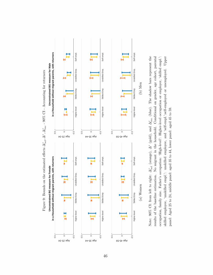
8.2. The contribution of returners

The estimation of ∆rsel, ∆r and ∆r

inc helps understanding the contribution of re-

turners to the human capital in the sending country. Students are overrepresented

among returners. This fact leads Baizan, Beauchemin, and Gonzalez-Ferrer (2013) to

conclude that “brain drain appears to be a limited issue in the context of Senegalese

migration”. Figure 9 depicts the change in the Brain Drain measures when one also

accounts for the human capital brought back by the returners. There is hardly any

change observed, suggesting that most returners would have acquired their education

even if they would have stayed in the origin country. This qualifies the hypothesis

that return migration might be a stronger channel for brain gain that the prospect of

emigration.

8.3. Households with a Migrant Member

Households with a migrant member are different in two respects; the absence of

a parent might have a negative effect on educational attainment (earlier entrance on

the labor market to substitute for loss in income, and lack of parental support) as

noted by for example by Hanson and Woodruff (2003). Conversely, remittances can

relax the liquidity constraint and allow more investment education. Dinkelman and

Mariotti (2014) and Theoharides (2015) finds that the income effect overcomes the

absent parent effect. Consistent with this findings, our sample shows that, in families

with a member abroad, one out four children is enrolled in upper secondary school,

against one out five in the remaining families.

29

Figure 10 depicts the change in the estimated measures for families were at least

of one member was abroad when the respondent was 15 years old. If anything, the

selection effect is more pronounced among women with a family member abroad

than among their counterpart women without a family member abroad, but not

significantly. In contrast, the incentive effects are larger in these type of households,

both for men and women. In fact, for men, they are not anymore significantly different

from zero, in most cases. For men in the richest families, as well as most female in

the younger cohort, the 50% confidence regions are positive (not reported) and the

90% confidence region have a tilt toward positive values, suggesting a strictly positive

incentives.

As a result, the net effect is not significantly different from zero for men, and still

slightly negative for women. Thus, the investment in education of families with a

migrant member is less elastic to migration prospects than the one of families where

both parents are in Senegal. The income effect seems to offset the negative brain

gain effect. For comparison with BLV, I also conducted the same analysis considering

households with a migrant father or mother. The results do not change significantly.

8.4. Alternative education levels

In this section, I also investigate potential effects at alternative educational levels:

lower secondary and tertiary education. Even though the father’s occupation is only

measured when the individual is 15 years old, there should be high correlation with

the occupation at the point of enrollment in the lower secondary or tertiary level.

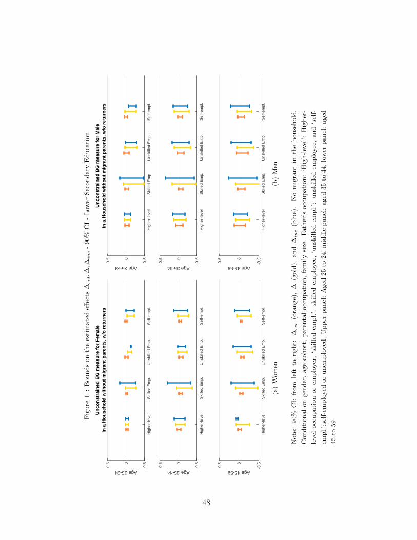
Start with the lower secondary school, fixing the family size at its median level

and focusing first on families were none of the parent was abroad when the respondent

was 15 years old. Figure 11 shows the same pattern as previously with respect to the

selection effect, except more noisy measures for men. Measures of the incentive effect

are also more noisy, but mainly not statistically different from zero, both for men and

women, with the notable exception of households from the youngest cohort with a

self-employed father or an unskilled father. In these groups, the incentive effects are

negative, both for men and women. Hence, the net effect is again negative for women,

mostly in the youngest cohort. For men, the effect is not significantly different from

zero, however, the confidence regions for the cohort 25-34 have a tilt toward negative

values.

30

The picture is very similar when one considers tertiary education (Figure 12).

The selection effect is negative or not significantly different from zero, and more pro-

nounced for rich families. The incentive effects display large bounds mainly centered

around zero. Finally, the net effects are negative for women, and for men, the con-

fidence regions for the cohort 25-34 have a tilt toward negative values, although not

significant.

Finally, note that families with a migrant member have again higher incentives

effects. At the secondary level, for men and women, all confidence intervals show a

tilt toward the positive values. At the tertiary level, the incentives for men from the

richest households are significantly positive, balancing the selection effect.

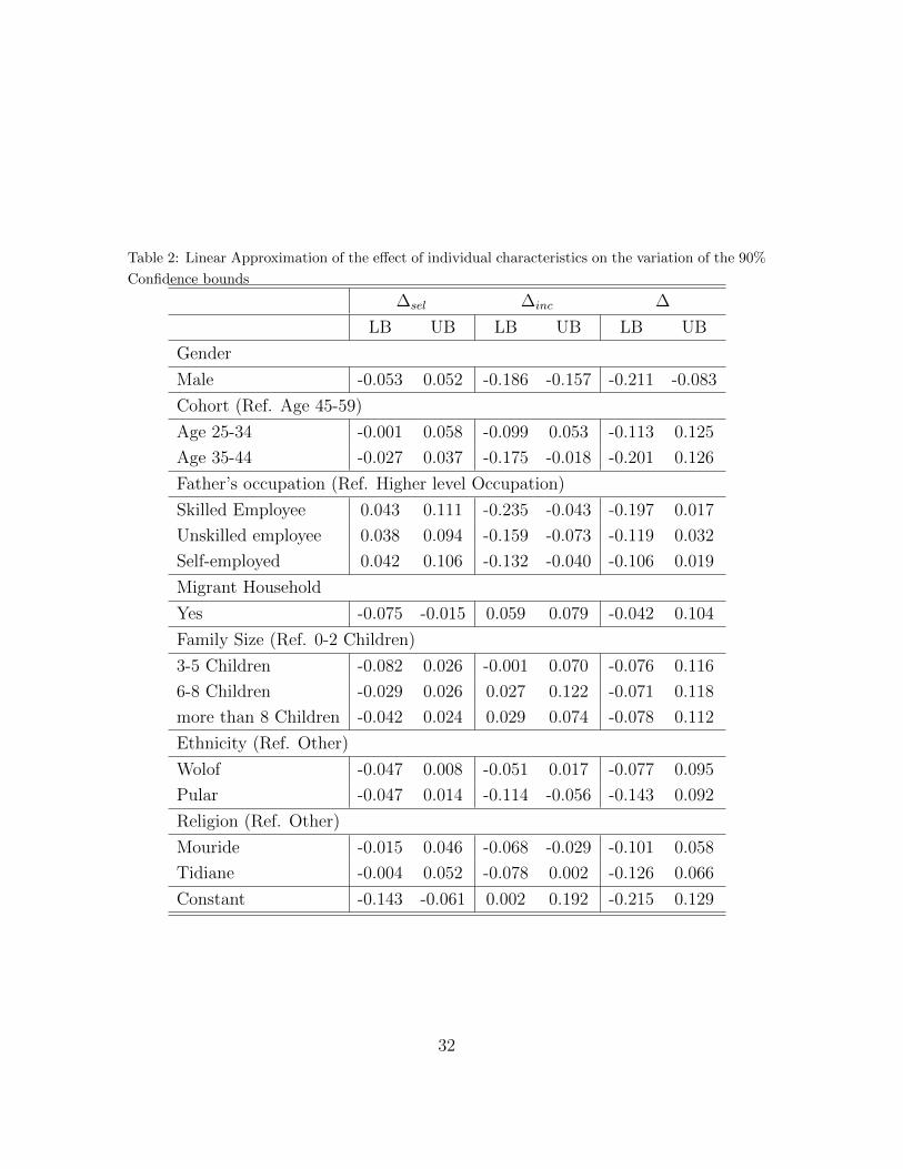
8.5. Linear Approximation

A parsimonious way to summarize the information conveyed by the bounds is to

compute a linear approximation of the variation of the measured effects, as described

in Appendix E. Table 2 summarizes the influence of the explanatory variables on the

measured effects, according to the linear approximation. This approach being more

flexible than the graphical approach, I control additionally for religious and ethnic

characteristics, additional proxies for migrant networks.

The reference group is women from the earliest cohort, whose father had a higher-

level occupation when they were aged 15, in small size families, from other ethnicity

and religion than the main ethnic and religious groups in Senegal. In this group, the

selection effect is strongly negative (see constant), with a decrease of upper secondary

school attendance between 6 to 14 percentage points. Families with a migrant member

are even more likely to experience the negative selection effect, of at least 1 additional

percentage point. The selection seems not to differ with respect to gender, ethnic

group or religion. However, less well-off families are not likely to experience the

negative selection effect.

By contrast, there is more variation in the incentive effects depending on the in-

dividual characteristics. The reference group has positive (possibly strong incentives)

to invest in education. Being a male candidate appears to deters substantially the

incentive effect (a decrease between 15 to 19 percentage points), as well as belonging

to less well-off families (a decrease between 4 to 23 percentage points), or religious and

ethnic networks. The medium cohort, where the liquidity constraint was presumably

31

Table 2: Linear Approximation of the effect of individual characteristics on the variation of the 90%

Confidence bounds

∆sel ∆inc ∆

LB UB LB UB LB UB

Gender

Male -0.053 0.052 -0.186 -0.157 -0.211 -0.083

Cohort (Ref. Age 45-59)

Age 25-34 -0.001 0.058 -0.099 0.053 -0.113 0.125

Age 35-44 -0.027 0.037 -0.175 -0.018 -0.201 0.126

Father’s occupation (Ref. Higher level Occupation)

Skilled Employee 0.043 0.111 -0.235 -0.043 -0.197 0.017

Unskilled employee 0.038 0.094 -0.159 -0.073 -0.119 0.032

Self-employed 0.042 0.106 -0.132 -0.040 -0.106 0.019

Migrant Household

Yes -0.075 -0.015 0.059 0.079 -0.042 0.104

Family Size (Ref. 0-2 Children)

3-5 Children -0.082 0.026 -0.001 0.070 -0.076 0.116

6-8 Children -0.029 0.026 0.027 0.122 -0.071 0.118

more than 8 Children -0.042 0.024 0.029 0.074 -0.078 0.112

Ethnicity (Ref. Other)

Wolof -0.047 0.008 -0.051 0.017 -0.077 0.095

Pular -0.047 0.014 -0.114 -0.056 -0.143 0.092

Religion (Ref. Other)

Mouride -0.015 0.046 -0.068 -0.029 -0.101 0.058

Tidiane -0.004 0.052 -0.078 0.002 -0.126 0.066

Constant -0.143 -0.061 0.002 0.192 -0.215 0.129

32

binding for most households, seems to have the lowest incentives of the three cohorts.

Conversely, households with a migrant have on average higher incentives (an increase

between 6 to 8 percentage points), so do larger families, compare to smaller families.

Given these variations in sometimes opposite direction, the resulting variations in

the net effect depend mainly on the gender, and at a lesser extent on the father’s

occupation. Hence, decomposing the net effect in selection and incentive effects, and

examining sub-groups of the population, reveal substantial variations that would pass

unnoticed when focusing solely on the country-level brain drain measures.

9. Discussion: Why are Men not Investing in Education?

The results of the empirical analysis suggest that emigration provides significant

disincentives for Senegalese men to invest in high school education. In this section, I

assess the possible reasons why it would be the case.

The first fact that demands explanation is the significant gender difference in

these incentives. The fact that emigration prospects produce no incentive for women

can be explained by the role of women in Senegalese households. Female have a

traditional role as wives and care takers at home, and a large differential social status

with respect to men (Barou, 1991; Baizan, Beauchemin, and Gonzalez-Ferrer, 2013).

Figure 2 which compares the reason of a migration by gender confirms this insight.

While men are more likely to migrate for work related reason or to improve their

living conditions, the large majority of women seems to be tied-movers as they report

migrating because of family reasons. Thus, it is not surprising that the incentive

effect does not operate on most of them.

Why do emigration prospects cause disincentives to invest in education in Senegal?

The literature evokes three potential reasons that I examine. The first potential reason

is that households compare relative returns to education rather than absolute returns

to education, as the Borjas-Roy model suggests (Borjas, 1987). In Equation (4), this

would mean that Π has a log-linear approximation. Since, relative returns are higher

in Sub-Saharan African countries than in OECD countries [REF], the additional

returns to education from emigration prospects should be negative. The hypothesis

of a log-linear utility function is however disputed in the context of migration from

developing to developed countries. Grogger and Hanson (2011) note that “given the

33

vast income differences that exist between countries [...] [the] linear utility appears

to abuse reality less than the strong curvature of the log-linear utility”. BLV also

favor the idea that absolute returns to education matter more than relative returns,

in the case of Cape Verde, the neighbor country of Senegal. Furthermore, since

relative returns to education increase exponentially in education in Senegal (Kuepie,

Nordman, and Roubaud, 2009), the disincentives should be higher at the tertiary level,

which is not the case. Therefore, the higher relative returns to education cannot solely

account for the negative incentives.

The second mechanism that could explain the negative incentives is the existence

of liquidity constraints for households with an emigration option, as described in

Section 3.3. Consistent with this mechanism, the results show that less well-off family

have the strongest disincentives, while the richest households have sometimes strictly

positive incentives. Moreover, households with a migrant, that presumably benefit

from remittances, are more likely to have positive incentive effects. This explanation

is also consistent with the finding that the incentive effects are the most negative for

the medium cohort. Thus, liquidity-constrained households appear to substitute the

investment in education for an investment in migration.

Third and final, the high prevalence of illegal migration or migration to low-

skill jobs may explain the negative incentives. This is consistent with the observed

negative effects of ethnic and religious networks that provide help to access low-skilled

occupations abroad [REF NEEDED]. This would also be consistent with the higher

incentives of households with a migrant, since these particular households would be

more likely to attempt migration through legal ways. However, contrary to what we

may have expected, the incentives do not seem to have significantly worsen in the

last cohort, where illegal migration is the most prevalent. To further assess whether

the observed negative incentives originate from low-skill job perspectives, I compare

the factual average level of occupation of migrants to the average level of occupation

in the counterfactual closed economy. To do so, I use the information in the survey

about the occupation level at age 35, as measured by the ISCO-code or the ISEI-

code of the occupation.20 Obviously, this can only be computed for the two earliest

20I do not use the occupation level at age 25, which is not a good proxy for the long-run labor mar-

ket outcomes. Indeed, Beauchemin et al. (201x) note that migrants have a significant occupational

34

cohorts. I define as high-skilled occupations, and denote by HSO = 1, occupations

with an ISCO-code below 5000, or occupations with an ISEI-code larger than 44.

Each partition gives us a proportion of approximately 20% of the population being

high-skilled, consistent with the proportion of men with upper secondary occupation.

Then, for men, I test respectively at the 5% level:

Ha0 : E(HSO|Y = 1, X)− E(HSO(0)|X) ≤ 0

Hb0 : E(HSO|Y = 1, X)− E(HSO(0)|X) ≥ 0

where HSO(0) is the occupation level of occupation in the closed economy. Using the

ISCO-code, Ha0 is never rejected, whereas Hb

0 is rejected in 2 groups out of 8. Using

the ISEI-code, Ha0 is rejected in 1 group out of 8, whereas Hb

0 is rejected in 6 groups

out of 8. Thus, it appears that emigration does not necessarily leads to lower types

of occupations than the ones expected in Senegal.

Hence, illegal migration and migration to low-skill jobs might partly explain the

negative incentive effects observed; however, financial constraints seem to be the main

driver of the finding.

10. Summary

This paper measured heterogeneous effects of emigration prospects on the school-

ing investment of households in Senegal. I derived bounds on the magnitude of these

effects from an IV discrete choice model that distinguishes migration decision and

actual migration. Using the MAFE Survey on Senegal reveals strong gender differ-

ence in incentives: I find strong disincentives for men to invest in education. The

most plausible explanation is that credit constraints leads to a substitution between

migration and education investments. Thus, in the absence of migration opportunity,

more men would have acquired secondary education.

Should the policy makers then increase the costs of migration? A marginal increase

has unclear effect. While it will deter the migration incentives for some, it will worsen

the liquidity constraint for others, possibly worsening the perverse effect of the market

imperfection. Furthermore, the stories of thousands who risk their lives on their way

costs in the first years following migration. However, this costs reduces rapidly overtime.

35

to Europe should teach us that it is difficult to set migration costs high enough to deter

all migration attempts. A better approach could be to focus on the credit market

inefficiency, while promoting human capital accumulation. This could be done by

creating legal and selective ways for economic migration,that can be financed on a

credit market.

References

Baizan, P., C. Beauchemin, and A. Gonzalez-Ferrer (2013): “Determinants

of migration between Senegal and France, Italy and Spain,” MAFE Project Working

Paper No. 25, January.

Barou, J. (1991): “L’immigration Africaine au Feminin,” Informations Sociales,

(14), 26–32.

Batista, C., A. Lacuesta, and P. C. Vicente (2012): “Testing the brain gain

hypothesis: Micro evidence from Cape Verde,” Journal of Development Economics,

97(1), 32–45.

Beauchemin, C. (2012): “Migrations between Africa and Europe: Rationale for a

survey design,” MAFE Methodological Note, (5).

Beine, M., F. Docquier, and H. Rapoport (2001): “Brain drain and economic

growth: theory and evidence,” Journal of development economics, 64(1), 275–289.

(2008): “Brain drain and human capital formation in developing countries:

Winners and losers,” The Economic Journal, 118(528), 631–652.

Bhagwati, J., and K. Hamada (1974): “The brain drain, international integration

of markets for professionals and unemployment: a theoretical analysis,” Journal of

Development Economics, 1(1), 19–42.

Borjas, G. J. (1987): “Self-Selection and the Earnings of Immigrants,” American

Economic Review, 77(4), 531–53.

Chand, S., and M. A. Clemens (2008): “Skilled emigration and skill creation: a

quasi-experiment,” Working Paper No. 152, September.

36

Chernozhukov, V., W. Kim, S. Lee, and A. Rosen (2013): “Implementing

intersection bounds in Stata,” Stata Journal, 15(1), 21–44.

Chernozhukov, V., S. Lee, and A. Rosen (2013): “Intersection Bounds: Esti-

mation and Inference,” Econometrica, 81(2), 667–737.

Chesher, A., and A. Rosen (2012): “Simultaneous Equations Models for Dis-

crete Outcomes, Coherence, Completeness and Identification,” Working Papers

CWP21/12, cemmap.

Dahl, G. B. (2002): “Mobility and the return to education: Testing a Roy model

with multiple markets,” Econometrica, 70(6), 2367–2420.

Dinkelman, T., and M. Mariotti (2014): “What are the long run effects of labor

migration on human capital? Evidence from Malawi,” unpublished manuscript.

Docquier, F., and A. Marfouk (2006): International migration by education

attainment, 1990-2000. in (C. Ozden and M. Schiff, eds.), International Migration,

Brain Drain and Remittances, pp. 15199, New York:, Palgrave Macmillan.

Docquier, F., and H. Rapoport (2012): “Globalization, brain drain, and devel-

opment,” Journal of Economic Literature, pp. 681–730.

Easterly, W., and Y. Nyarko (2008): “Is the brain drain good for Africa?,”

Brookings Global Economy and Development Working Paper, (19).

Gibson, J., and D. McKenzie (2011a): “Eight questions about brain drain,” The

Journal of Economic Perspectives, pp. 107–128.

(2011b): “The microeconomic determinants of emigration and return migra-

tion of the best and brightest: Evidence from the Pacific,” Journal of Development

Economics, 95(1), 18–29.

Girsberger, E. M. (2014): “Migration, Education and Work Opportunities,” un-

published manuscript.

Grogger, J., and G. H. Hanson (2011): “Income maximization and the selection

and sorting of international migrants,” Journal of Development Economics, 95(1),

42–57.

37

Hanson, G. H., and C. Woodruff (2003): “Emigration and educational attain-

ment in Mexico,” unpublished manuscript.

Heckman, J. J., and E. Vytlacil (2001): “Policy-relevant treatment effects,”

American Economic Review, pp. 107–111.

Heckman, J. J., and E. J. Vytlacil (2007): “Econometric evaluation of social

programs, part I: Causal models, structural models and econometric policy evalu-

ation,” Handbook of econometrics, 6, 4779–4874.

Kapur, D., and J. McHale (2005): Give us your best and brightest: The global

hunt for talent and its impact on the developing world. Ctr for Global Development.

Katz, E., and H. Rapoport (2005): “On human capital formation with exit

options,” Journal of Population Economics, 18(2), 267–274.

Kuepie, M., C. J. Nordman, and F. Roubaud (2009): “Education and earnings

in urban West Africa,” Journal of Comparative Economics, 37(3), 491–515.

Lacomba, J., and A. Moncusı (2006): “Senegaleses en la Comunidad Valenciana:

redes, cofradıas y venta ambulante,” Jabardo M., Senegaleses en Espana. Conex-

iones entre origen y destino, Madrid: Ministerio de trabajo y asuntos sociales, pp.

74–78.

Manski, C. (1993): “Identification of endogenous social effects: the reflection prob-

lem,” Review of Economic Studies, 60, 531–542.

Mbaye, L. M. (2014): ““Barcelona or die”: understanding illegal migration from

Senegal,” IZA Journal of Migration, 3(1), 1–19.

McKenzie, D., and H. Rapoport (2011): “Can migration reduce educational

attainment? Evidence from Mexico,” Journal of Population Economics, 24(4),

1331–1358.

Mountford, A. (1997): “Can a brain drain be good for growth in the source

economy?,” Journal of development economics, 53(2), 287–303.

Mourifie, I., M. Henry, and R. Meango (2015): “Sharp Bounds for the Roy

Model,” unpublished manuscript.

38

Obucina, O. (2013): “Occupational trajectories and occupational cost among Sene-

galese immigrants in Europe,” Demographic Research, 28(19), 547–580.

Robin, N. (1996): Atlas des migrations ouest-africaines vers l’Europe, 1985-1993.

IRD Editions.

Rosenzweig, M. R. (2008): “Higher Education and International Migration in Asia:

Brain Circulation,” in Annual World Bank Conference on Development Economics,

pp. 59–100.

Shrestha, S. A. (2015): “No Man Left Behind: Effects of Emigration Prospects on

Educational and Labor Outcomes of Non-migrants,” unpublished manuscript.

Stark, O., C. Helmenstein, and A. Prskawetz (1997): “A brain gain with a

brain drain,” Economics letters, 55(2), 227–234.

Steinmayr, A. (2014): “When a random sample is not random: Bounds on the

effect of migration on household members left behind,” No. 1975. Kiel Working

Paper.

Theoharides, C. (2015): “Manila to Malaysia, Quezon to Qatar: International

Migration and the Effects on Origin-Country Human Capital,” .

Willis, R., S. Rosen, and J. Heckman (1979): “Education and Self-Selection,”

Journal of Political Economy, 87.

39

Figure 1: Migration attempts and migration success

0.75

.5.2

50

.25

.5.7

5A

ttem

pts

and

Act

ual M

igra

tion

rate

s

Primary Lower Sec. Upper Sec. TertiaryEducation

Attempts Men Attempts WomenMig. Men Mig. Women

Note: Proportion of the population who attempted migration to Europe and the

proportion of those who have been successful, by gender and education level. ‘At-

tempts Men/Women’: Estimated proportion in the population who attempted

migration. ‘Mig Men/Women’: Estimated proportion in the population that

migrated to Europe. Education: ‘Primary’: Primary or Less than Primary,

‘Lower Sec.’ some Lower Secondary, ‘Upper Sec.’: some Upper Secondary, and

‘Tertiary’: some Tertiary education. The bars represent the 95% Confidence

Interval.

40

Figure 2: Reason of emigration

.5.2

50

.25

.5

Family Work education Living Conditions OtherReason of Migration

Male Female

Note: Main stated reason of emigration by gender. ‘Living condition’ stands for

‘Improving or find better living conditions’.

Figure 3: Age at first migration attempt, for migrants and non-migrants

0.0

2.0

4.0

6.0

8

20 30 40 50x

Non−Migrants Migration to Europe

Note: Kernel distribution of the age at the first migration attempt, conditional

on having attempted migration for the first time, after the age of 21, and on the

migration status.

41

Figure 4: Age at migration, by gender

0.0

2.0

4.0

6.0

8kd

ensi

ty a

ge_a

t_m

igra

tion

20 30 40 50 60x

Men WomenAll

Note: Kernel distribution of the age at the first migration attempt, conditional

on migration for the first time, after the age of 21, and on the gender.

Figure 5: Age at migration, by education

0.0

2.0

4.0

6.0

8.1

kden

sity

age

_at_

mig

ratio

n

20 30 40 50 60x

Primary Lower Sec.Upper Sec. Tertiary

Note: Kernel distribution of the age at the first migration attempt, conditional

on migration for the first time, after the age of 21, and on the educational

attainment. Education: ‘Primary’: Primary or Less than Primary, ‘Lower Sec.’

some Lower Secondary, ‘Upper Sec.’: some Upper Secondary, and ‘Tertiary’:

some Tertiary education.

42

Figure 6: Education by gender, cohort and migration status

0.75

.5.2

50

.25

.5.7

5E

duca

tiona

l atta

inm

ent r

ates

Primary Lower Sec. Upper Sec. TertiaryEducation

Non−mig. Men Non−mig. WomenMig. Men Mig. Women

(a) Age cohort 25-34

0.75

.5.2

50

.25

.5.7

5E

duca

tiona

l atta

inm

ent r

ates

Primary Lower Sec. Upper Sec. TertiaryEducation

Non−mig. Men Non−mig. WomenMig. Men Mig. Women

(b) Age cohort 35-44

0.75

.5.2

50

.25

.5.7

5E

duca

tiona

l atta

inm

ent r

ates

Primary Lower Sec. Upper Sec. TertiaryEducation

Non−mig. Men Non−mig. WomenMig. Men Mig. Women

(c) Age cohort 45-59

Note: Estimated distribution of education, conditional on migration status, age

cohort and gender. Education: ‘Primary’: Primary or Less than Primary, ‘Lower

Sec.’ some Lower Secondary, ‘Upper Sec.’: some Upper Secondary, and ‘Ter-

tiary’: some Tertiary education. The bars represent the 95% Confidence Interval.

43

Fig

ure

7:

Bou

nd

son

the

esti

mate

deff

ects

∆sel,

∆,∆

inc

-50%

CI

Hig

her-

leve

lS

kille

d E

mp.

Uns

kille

d E

mp.

Sel

f-em

pl.

Age 25-34 -0.50

0.5

Un

con

stra

ined

BG

mea

sure

fo

r F

emal

e in

a H

ou

seh

old

wit

ho

ut

mig

ran

t p

aren

ts, w

/o r

etu

rner

s

Hig

her-

leve

lS

kille

d E

mp.

Uns

kille

d E

mp.

Sel

f-em

pl.

Age 35-44 -0.50

0.5

Hig

her-

leve

lS

kille

d E

mp.

Uns

kille

d E

mp.

Sel

f-em

pl.

Age 45-59 -0.50

0.5

(a)

Wom

en

Hig

her-

leve

lS

kille

d E

mp.

Uns

kille

d E

mp.

Sel

f-em

pl.

Age 25-34 -0.50

0.5

Un

con

stra

ined

BG

mea

sure

fo

r M

ale

in a

Ho

use

ho

ld w

ith

ou

t m

igra

nt

par

ents

, w/o

ret

urn

ers

Hig

her-

leve

lS

kille

d E

mp.

Uns

kille

d E

mp.

Sel

f-em

pl.

Age 35-44 -0.50

0.5

Hig

her-

leve

lS

kille

d E

mp.

Uns

kille

d E

mp.

Sel

f-em

pl.

Age 45-59 -0.50

0.5

(b)

Men

Not

e:50

%C

I:fr

omle

ftto

right:

∆sel

(ora

nge)

,∆

(gold

),an

d∆

inc

(blu

e).

No

mig

rant

inth

eh

ou

seh

old

.

Con

dit

ion

alon

gen

der

,ag

eco

hort

,p

are

nta

locc

up

ati

on

,fa

mil

ysi

ze.

Fath

er’s

occ

up

ati

on

:‘H

igh

-lev

el’:

Hig

her

-

leve

locc

up

atio

nor

emp

loye

r,‘s

kil

led

emp

l.’:

skil

led

emp

loye

e,‘u

nsk

ille

dem

pl.

’:u

nsk

ille

dem

plo

yee

,an

d‘s

elf-

emp

l.’:

self

-em

plo

yed

oru

nem

plo

yed

.U

pp

erp

an

el:

Aged

25

to24,

mid

dle

pan

el:

aged

35

to44,

low

erp

an

el:

aged

45to

59.

44

Fig

ure

8:

Bou

nd

son

the

esti

mate

deff

ects

∆sel,

∆,∆

inc

-90%

CI

Hig

her-

leve

lS

kille

d E

mp.

Uns

kille

d E

mp.

Sel

f-em

pl.

Age 25-34 -0.50

0.5

Un

con

stra

ined

BG

mea

sure

fo

r F

emal

e in

a H

ou

seh

old

wit

ho

ut

mig

ran

t p

aren

ts, w

/o r

etu

rner

s

Hig

her-

leve

lS

kille

d E

mp.

Uns

kille

d E

mp.

Sel

f-em

pl.

Age 35-44 -0.50

0.5

Hig

her-

leve

lS

kille

d E

mp.

Uns

kille

d E

mp.

Sel

f-em

pl.

Age 45-59 -0.50

0.5

(a)

Wom

en

Hig

her-

leve

lS

kille

d E

mp.

Uns

kille

d E

mp.

Sel

f-em

pl.

Age 25-34 -0.50

0.5

Un

con

stra

ined

BG

mea

sure

fo

r M

ale

in a

Ho

use

ho

ld w

ith

ou

t m

igra

nt

par

ents

, w/o

ret

urn

ers

Hig

her-

leve

lS

kille

d E

mp.

Uns

kille

d E

mp.

Sel

f-em

pl.

Age 35-44 -0.50

0.5

Hig

her-

leve

lS

kille

d E

mp.

Uns

kille

d E

mp.

Sel

f-em

pl.

Age 45-59 -0.50

0.5

(b)

Men

Not

e:90

%C

I:fr

omle

ftto

right:

∆sel

(ora

nge)

,∆

(gold

),an

d∆

inc

(blu

e).

No

mig

rant

inth

eh

ou

seh

old

.

Con

dit

ion

alon

gen

der

,ag

eco

hort

,p

are

nta

locc

up

ati

on

,fa

mil

ysi

ze.

Fath

er’s

occ

up

ati

on

:‘H

igh

-lev

el’:

Hig

her

-

leve

locc

up

atio

nor

emp

loye

r,‘s

kil

led

emp

l.’:

skil

led

emp

loye

e,‘u

nsk

ille

dem

pl.

’:u

nsk

ille

dem

plo

yee

,an

d‘s

elf-

emp

l.’:

self

-em

plo

yed

oru

nem

plo

yed

.U

pp

erp

an

el:

Aged

25

to24,

mid

dle

pan

el:

aged

35

to44,

low

erp

an

el:

aged

45to

59.

45

Fig

ure

9:B

oun

ds

onth

ees

tim

ate

deff

ects

∆r sel,

∆r,∆

r inc

-90%

CI

-A

ccou

nti

ng

for

retu

rner

s

Hig

her-

leve

lS

kille

d E

mp.

Uns

kille

d E

mp.

Sel

f-em

pl.

Age 25-34 -0.50

0.5

Un

con

stra

ined

BG

mea

sure

fo

r F

emal

e in

a H

ou

seh

old

wit

ho

ut

mig

ran

t p

aren

ts, w

ith

ret

urn

ers

Hig

her-

leve

lS

kille

d E

mp.

Uns

kille

d E

mp.

Sel

f-em

pl.

Age 35-44 -0.50

0.5

Hig

her-

leve

lS

kille

d E

mp.

Uns

kille

d E

mp.

Sel

f-em

pl.

Age 45-59 -0.50

0.5

(a)

Wom

en

Hig

her-

leve

lS

kille

d E

mp.

Uns

kille

d E

mp.

Sel

f-em

pl.

Age 25-34 -0.50

0.5

Un

con

stra

ined

BG

mea

sure

fo

r M

ale

in a

Ho

use

ho

ld w

ith

ou

t m

igra

nt

par

ents

, wit

h r

etu

rner

s

Hig

her-

leve

lS

kille

d E

mp.

Uns

kille

d E

mp.

Sel

f-em

pl.

Age 35-44 -0.50

0.5

Hig

her-

leve

lS

kille

d E

mp.

Uns

kille

d E

mp.

Sel

f-em

pl.

Age 45-59 -0.50

0.5

(b)

Men

Not

e:90

%C

I:fr

omle

ftto

righ

t:∆

r sel

(ora

nge)

,∆

r(g

old

),an

d∆

r inc

(blu

e).

Th

esh

ad

owb

ars

rep

rese

nt

the

resu

lts

ofth

eb

asel

ine

esti

mat

ion

.N

om

igra

nt

inth

eh

ou

seh

old

.C

on

dit

ion

al

on

gen

der

,age

coh

ort

,p

are

nta

l

occ

up

atio

n,

fam

ily

size

.F

ath

er’s

occ

up

ati

on

:‘H

igh

-lev

el’:

Hig

her

-lev

elocc

up

ati

on

or

emp

loye

r,‘s

kil

led

emp

l.’:

skil

led

emp

loyee

,‘u

nsk

ille

dem

pl.

’:u

nsk

ille

dem

plo

yee,

an

d‘s

elf-

emp

l.’:

self

-em

plo

yed

or

un

emp

loyed

.U

pp

er

pan

el:

Age

d25

to24

,m

idd

lep

an

el:

aged

35

to44,

low

erp

an

el:

aged

45

to59.

46

Fig

ure

10:

Bou

nd

son

the

esti

mate

deff

ects

∆sel,

∆,∆

inc

-90%

CI

-H

ou

seh

old

sw

ith

am

igra

nt

Hig

her-

leve

lS

kille

d E

mp.

Uns

kille

d E

mp.

Sel

f-em

pl.

Age 25-34 -0.50

0.5

Un

con

stra

ined

BG

mea

sure

fo

r F

emal

e in

a H

ou

seh

old

wit

h m

igra

nt

par

ents

, w/o

ret

urn

ers

Hig

her-

leve

lS

kille

d E

mp.

Uns

kille

d E

mp.

Sel

f-em

pl.

Age 35-44 -0.50

0.5

Hig

her-

leve

lS

kille

d E

mp.

Uns

kille

d E

mp.

Sel

f-em

pl.

Age 45-59 -0.50

0.5

(a)

Wom

en

Hig

her-

leve

lS

kille

d E

mp.

Uns

kille

d E

mp.

Sel

f-em

pl.

Age 25-34 -0.50

0.5

Un

con

stra

ined

BG

mea

sure

fo

r M

ale

in a

Ho

use

ho

ld w

ith

mig

ran

t p

aren

ts, w

/o r

etu

rner

s

Hig

her-

leve

lS

kille

d E

mp.

Uns

kille

d E

mp.

Sel

f-em

pl.

Age 35-44 -0.50

0.5

Hig

her-

leve

lS

kille

d E

mp.

Uns

kille

d E

mp.

Sel

f-em

pl.

Age 45-59 -0.50

0.5

(b)

Men

Not

e:90

%C

I:fr

omle

ftto

righ

t:∆

sel

(ora

nge)

,∆

(gold

),an

d∆

inc

(blu

e).

Th

esh

ad

owb

ars

rep

rese

nt

the

resu

lts

ofth

eb

asel

ine

esti

mat

ion

.A

tle

ast

on

em

igra

nt

inth

eh

ou

seh

old

.C

on

dit

ion

al

on

gen

der

,age

coh

ort

,

par

enta

locc

up

atio

n,

fam

ily

size

.F

ath

er’s

occ

upati

on

:‘H

igh

-lev

el’:

Hig

her

-lev

elocc

up

ati

on

or

emp

loye

r,‘s

kil

led

emp

l.’:

skil

led

emp

loye

e,‘u

nsk

ille

dem

pl.

’:u

nsk

ille

dem

plo

yee,

an

d‘s

elf-

emp

l.’:

self

-em

plo

yed

or

un

emp

loye

d.

Up

per

pan

el:

Age

d25

to24

,m

idd

lep

an

el:

aged

35

to44,

low

erp

anel

:aged

45

to59.

47

Fig

ure

11:

Bou

nd

son

the

esti

mate

deff

ects

∆sel,

∆,∆

inc

-90%

CI

-L

ower

Sec

on

dary

Ed

uca

tion

Hig

her-

leve

lS

kille

d E

mp.

Uns

kille

d E

mp.

Sel

f-em

pl.

Age 25-34 -0.50

0.5

Un

con

stra

ined

BG

mea

sure

fo

r F

emal

e in

a H

ou

seh

old

wit

ho

ut

mig

ran

t p

aren

ts, w

/o r

etu

rner

s

Hig

her-

leve

lS

kille

d E

mp.

Uns

kille

d E

mp.

Sel

f-em

pl.

Age 35-44 -0.50

0.5

Hig

her-

leve

lS

kille

d E

mp.

Uns

kille

d E

mp.

Sel

f-em

pl.

Age 45-59 -0.50

0.5

(a)

Wom

en

Hig

her-

leve

lS

kille

d E

mp.

Uns

kille

d E

mp.

Sel

f-em

pl.

Age 25-34 -0.50

0.5

Un

con

stra

ined

BG

mea

sure

fo

r M

ale

in a

Ho

use

ho

ld w

ith

ou

t m

igra

nt

par

ents

, w/o

ret

urn

ers

Hig

her-

leve

lS

kille

d E

mp.

Uns

kille

d E

mp.

Sel

f-em

pl.

Age 35-44 -0.50

0.5

Hig

her-

leve

lS

kille

d E

mp.

Uns

kille

d E

mp.

Sel

f-em

pl.

Age 45-59 -0.50

0.5

(b)

Men

Not

e:90

%C

I:fr

omle

ftto

right:

∆sel

(ora

nge)

,∆

(gold

),an

d∆

inc

(blu

e).

No

mig

rant

inth

eh

ou

seh

old

.

Con

dit

ion

alon

gen

der

,ag

eco

hort

,p

are

nta

locc

up

ati

on

,fa

mil

ysi

ze.

Fath

er’s

occ

up

ati

on

:‘H

igh

-lev

el’:

Hig

her

-

leve

locc

up

atio

nor

emp

loye

r,‘s

kil

led

emp

l.’:

skil

led

emp

loye

e,‘u

nsk

ille

dem

pl.

’:u

nsk

ille

dem

plo

yee

,an

d‘s

elf-

emp

l.’:

self

-em

plo

yed

oru

nem

plo

yed

.U

pp

erp

an

el:

Aged

25

to24,

mid

dle

pan

el:

aged

35

to44,

low

erp

an

el:

aged

45to

59.

48

Fig

ure

12:

Bou

nd

son

the

esti

mate

deff

ects

∆sel,

∆,∆

inc

-90%

CI

-T

erti

ary

Ed

uca

tion

Hig

her-

leve

lS

kille

d E

mp.

Uns

kille

d E

mp.

Sel

f-em

pl.

Age 25-34 -0.50

0.5

Un

con

stra

ined

BG

mea

sure

fo

r F

emal

e in

a H

ou

seh

old

wit

ho

ut

mig

ran

t p

aren

ts, w

/o r

etu

rner

s

Hig

her-

leve

lS

kille

d E

mp.

Uns

kille

d E

mp.

Sel

f-em

pl.

Age 35-44 -0.50

0.5

Hig

her-

leve

lS

kille

d E

mp.

Uns

kille

d E

mp.

Sel

f-em

pl.

Age 45-59 -0.50

0.5

(a)

Wom

en

Hig

her-

leve

lS

kille

d E

mp.

Uns

kille

d E

mp.

Sel

f-em

pl.

Age 25-34 -0.50

0.5

Un

con

stra

ined

BG

mea

sure

fo

r M

ale

in a

Ho

use

ho

ld w

ith

ou

t m

igra

nt

par

ents

, w/o

ret

urn

ers

Hig

her-

leve

lS

kille

d E

mp.

Uns

kille

d E

mp.

Sel

f-em

pl.

Age 35-44 -0.50

0.5

Hig

her-

leve

lS

kille

d E

mp.

Uns

kille

d E

mp.

Sel

f-em

pl.

Age 45-59 -0.50

0.5

(b)

Men

Not

e:90

%C

I:fr

omle

ftto

right:

∆sel

(ora

nge)

,∆

(gold

),an

d∆

inc

(blu

e).

No

mig

rant

inth

eh

ou

seh

old

.

Con

dit

ion

alon

gen

der

,ag

eco

hort

,p

are

nta

locc

up

ati

on

,fa

mil

ysi

ze.

Fath

er’s

occ

up

ati

on

:‘H

igh

-lev

el’:

Hig

her

-

leve

locc

up

atio

nor

emp

loye

r,‘s

kil

led

emp

l.’:

skil

led

emp

loye

e,‘u

nsk

ille

dem

pl.

’:u

nsk

ille

dem

plo

yee

,an

d‘s

elf-

emp

l.’:

self

-em

plo

yed

oru

nem

plo

yed

.U

pp

erp

an

el:

Aged

25

to24,

mid

dle

pan

el:

aged

35

to44,

low

erp

an

el:

aged

45to

59.

49

Appendix

A. Point Identification with a LIV

The LIV requires (i) an approximation of the return to education through a la-

tent index equation, (ii) a monotonicity condition on the effect of the instrument(s)

and (iii) a set of instruments with a sufficiently large support. I view this set of

assumptions as untenable in the present framework.

First, it is not clear whether the migration decision can be described by a latent

index equation of the form:

Y ∗ = I (µ(W,Z) > U) (A.1)

where U is uniformly distributed on the unit interval and stochastically independent of

Z (an instrument) conditional on W . Indeed, Y ∗ depends on the choice of education

through the succes probability pd and the net returns to emigration (gains minus

costs). So that, if the true specification would be:

Y ∗ = I (µ∗(D,W,Z) > U∗) (A.2)

the independence condition would require that U = U∗ + µ∗(D,W,Z) − µ(W,Z) be

independent of Z, a particular case.

Second, it is not clear whether the instrumental variables in the present context

satisfy the monotonicity condition required by the latent index model. Following

BLV, I use the length of the longest spell of migration among household members

to instrument the migration decision. As explained below, a longer migration spell

should influence positively the migration decision in general. According to the mono-

tonicity assumption, the (weak) increase in the migration decision should then take

place for all individuals. There is however reasons to think that longer migration

spells would imply weaker ties for some families, decreasing instead the migration

propensity for these particular families.

Finally, to attain point identification Z should drive the probability of attempting

migration to zero. However, it is hard to believe that the instruments in the present

context would induce such variations on the migration decision.

50

B. Non-Redundent Restrictions on ∆

Consider ∆:

∆ = E(D|Y = 0)− ED(0)

= P (D = 1, Y ∗ = 0|Y = 0) + P (D = 1, Y ∗ = 1|Y = 0)− ED(0)

= P (D = 1, Y ∗ = 0, Y = 0)/P (Y = 0) + P (D = 1, Y ∗ = 1, Y = 0)/P (Y = 0)− ED(0)

= P (D = 1, Y ∗ = 0)/P (Y = 0) + P (D = 1, Y ∗ = 1, Y = 0)/P (Y = 0)− ED(0)

where the last line is the consequence of

Y ∗ = 0⇒ Y = 0. (B.1)

Since:

ED(0) = P (D(0) = 1, Y ∗ = 0) + P (D(0) = 1, Y ∗ = 1)

= P (D = 1, Y ∗ = 0) + P (D(0) = 1, Y ∗ = 1)(B.2)

It follows that:

∆ = P (D = 1, Y ∗ = 0) [1/P (Y = 0)− 1] + P (D = 1, Y ∗ = 1, Y = 0)/P (Y = 0)

−P (D(0) = 1, Y ∗ = 1)

As 0 ≤ P (D(0) = 1, Y ∗ = 1) ≤ P (Y ∗ = 1), ∆ must satisfy:

∆ ≤ P (D = 1, Y ∗ = 0) [1/P (Y = 0)− 1] + P (D = 1, Y ∗ = 1, Y = 0)/P (Y = 0)

∆ ≥ P (D = 1, Y ∗ = 0) [1/P (Y = 0)− 1] + P (D = 1, Y ∗ = 1, Y = 0)/P (Y = 0)

−P (Y ∗ = 1)

(B.3)

C. Instrument: index measure interacting the network and the unemploy-

ment rate

To take advantage of exogenous variations that affect the returns to education

abroad but not at home, I construct an index measure, which interacts, at a given

age, the strength of a network in one of the three destinations and the unemployment

rate in this location.

Let Nc,t,i be the size of i’s network in country c when he is aged t. Let Uc,t,i be

the unemployment rate by gender for individual between 25 to 34, in country c when

i is aged t. The index I construct takes the following form:

Ii =1

6

∑16≤t≤21

∑c∈{FR,IT,ES} Uc,t,i(Nc,t,i + 1)∑

c∈{FR,IT,ES}(Nc,t,i + 1)

When the data on unemployment rate are missing for a given country, I replace

them by the OECD average. In particular, all three series start after 1972.

51

D. Implementing the Command clr3bound

The command clr3bound is part of the Stata Package clrbound provided by Cher-

nozhukov, Kim, Lee, and Rosen (2013). clr3bound constructs confidence intervals

of level 1 − α by inverting a statistical test of corresponding level. It requires three

inputs for each the lower and upper bound: the dependent variables, the control and

instrument variables, and the range over which the optimization is to be performed.

D.1. Dependent Variables

Take the Lower bound on ∆(X), that is E(D|Y = 0, X) − UB0(X), where

UB0(X) = 1 − ˜q00. First, to circumvent the curse of dimensionality, I approximate

E(D|Y = 0, X) with E(D|Y = 0, X) = P (D, Y = 0|X)/P (Y = 0|X) using Linear

Probability Models for the numerator and the denominator. E(D|Y = 0, X) is then

used as a Plug-in estimator as advised by Mourifie, Henry, and Meango (2015).

As in ?, the dependent variable is defined as E(Di|Yi = 0, Xi) − (1 − I(Di =

0, Y ∗i = 0)), where I(D = 0, Y ∗ = 0) = 1 if the i’s Education is D = 0 and i never

attempted migration.

The remaining bounds are constructed accordingly.

D.2. Control and instrumental variables

I list in the command clr3bound, the control and instrumental variables in Section

7.2 and 7.3. Note that estimation is conducted separately for men and women. When

a polynomial specification of the instrument is considered, further exponents of the

instrumental variables are introduced up to degree 5. In the reported results, I use

the degree 3.

D.3. Range

The range matrix to be imputed in the command clr3bound is defined by producing

combinations of the instrumental variables. In the baseline, I use the “Network

innovation between 16 and 21” and the “Index measure”. I demean each of these

variables. I use an eight points for the first instrument and a 25 grid points for the

second instrument. When a polynomial specification of the instrument is considered,

further exponents of the range are introduced up to degree 5. In the reported results,

I use the degree 3.

52

E. Linear Approximation

The information conveyed by the variation of bounds can be usefully summarized

by using a linear approximation of the variation of the measured effects. Denote

by LB∆(X) (respectively UB∆(X)) the lower (resp. upper) bound estimated on

the measure ∆. And denote the estimated bounds on ∆sel, or ∆inc correspondingly.

Assume that there exists some real vector β∆ such that:

LB∆(X) ≤ Xβ∆ ≤ UB∆(X) (E.1)

The range of each component of the vector β∆ can be obtained by solving two lin-

ear programming problems: the first one minimizes the component of β∆,j under

the inequality constraints (E.1) and the second one maximizes β∆,j under the same

constraints.

The solutions of these optimization problems are presented in Table 2. Note

that the results do not give the 90% confidence interval an hypothetical parameter

β∆ such that ∆(X) = Xβ∆. This is because each confidence interval is computed

separetely. Ideally, one should construct first joint confidence region for all X and run

the procedure. This is not feasible with the Stata package, because of computational

restrictions.

F. Refinements Using the Migration Status

Prior information on the sign of the returns to education can be used to refined the

bounds. Moreover, these refined bounds allow to falsify assumptions on the returns

to education. The data at hand allow to identify migrants without legal documents at

their first migration. Therefore, I consider four possible assumptions on the returns

to education, depending on the type of migration.

Assumption 1. Assume that either:

1. For any household, the returns to education in case of illegal migration are lowerthan the returns to education in the origin country;

2. For any household, the returns to education in case of legal migration are higherthan the returns to education in the origin country;

3. For any household, the returns to education in case of illegal migration are lowerthan the returns to education in the origin country, and the returns to educationin case of legal migration are higher than the returns to education in the origincountry;

53

4. For any household, the returns to education in case of migration (legal or illegal)are higher than the returns to education in the origin country.

Assumption 1.1 states that for any randomly chosen household, illegal migration

results in disincentives to invest in education, and follows from our previous discussion

on illegal migration. Conversely, Assumption 1.2 states that legal migration provides

incentive to invest in education. Assumption 1.3 claims both. Finally, Assumption

1.4 claims that incentives are always positive. From the discussion in Section 3.3,

it should not hold in all subgroups. Assumption 1.4 should be seen as the most

optimistic case for finding a net positive effect, that is because the incentive effect

given by emigration prospects operates on all individuals in the population.

F.1. Bounds on ED(0)

Refined bounds can be derived on the counterfactual quantity ED(0), under the

different scenarios in Assumption 1. To state this bounds, it is necessary to introduce

additional notations to distinguish legal and illegal migration spells. Still denoting

by Y ∗ the migration decision, Y ∗ can take one of the three following values: Y ∗ = 0,

if the household decides not to attempt migration, Y ∗ = 1l if the household decides

to attempt legal migration, and Y ∗ = 1i if the household decides to attempt illegal

migration. Then, the bounds on ED(0) are given by the following proposition:

Proposition 2. Assume that D(0) is stochastically independent from Z :=(Z,X(1), Z(1)

),

conditionally on X, and the following expressions are well defined.

q1 := inf{ P(D = 1|Z = z) : z ∈ Supp(Z)},q00−01l := inf{ P(D = 0, Y ∗ = 0|Z = z) + P(D = 0, Y ∗ = 1l|Z = z) : z ∈ Supp(Z)},˜q10−11i := inf{ P(D = 1, Y ∗ = 0|Z = z) + P(D = 1, Y ∗ = 1i|Z = z) : z ∈ Supp(Z)}.

Under Assumption 1.1:

˜q10−11i ≤ ED(0) ≤ 1− ˜q00 (F.1)

Under Assumption 1.2:˜q10 ≤ ED(0) ≤ 1− q00−01l (F.2)

Under Assumption 1.3:

˜q10−11i ≤ ED(0) ≤ 1− q00−01l (F.3)

Finally, Under Assumption 1.4:

˜q10 ≤ ED(0) ≤ q1 (F.4)

54

To understand the bounds above, it is useful to resort to an alternative interpre-

tation. For example, Assumption 1.4 rules out the possibility that an individual who

would have obtained education D = 1 when Y ∗ = 0, would not obtain the same

level of education when Y ∗ ∈ 1i, 1l. An individual with such behavior is known in

the potential outcome literature has a “defier”.21 Assumption 1.4 can therefore be

interpreted as a “No-defier” assumption.

Each of these bounds has at least two use. First, they provide testable implications

for the different scenarios in Assumption 1. Indeed if for example, under Assump-

tion 1.4, the lower and the upper bound cross each other, the hypothesis of positive

incentives for all households is rejected by the data. Second, even if the bounds do

not cross, they provide an interpretation in terms of the proportion of defiers needed

to revert the estimated net effect. For example, assume that under the No-defier

Assumption, the lower bound on ∆(x) = b, where 0 < b < 1. If defiers are rule out,

then we should unambiguously conclude to a net brain gain in the sub-group x. If

one does not rule out the existence of defiers, b represents the proportion of defiers

that is needed in the sub-population of individuals with characteristics x to refute

the hypothesis of a net positive effect in the sub-population of interest. The higher

b, the more credible is the conclusion of a net brain gain.

F.2. Results under Assumption 1

Assumption 1.4 is readily rejected, since the unrestricted bounds derived in Section

8 show that some sub-groups have on average negative incentive effects. The inference

procedure also rejects Assumption 1.1 and, hence Assumption 1.3, for men in the

youngest cohort and men from the richest families. In other words, despite their

status as illegal migrants, some individuals in these sub-groups receive additional

incentives to invest in education from emigration prospects. The proportion of these

individuals is the largest among the richest household: at least 11% of the Senegalese

in the youngest cohort and richest families have positive returns to illegal migration.

Interestingly, Assumption 1.4 is rejected when one considers Tertiary education, but

not Assumption 1.3.

21The other possible categories comprise (i) the never-taker who never obtain education D = 1

irrespective of their migration decision, (ii) the always-taker who always obtain education D = 1

irrespective of their migration decision, and (iii) the compliers who obtain education D = 1 if and

only if they decide to migrate.

55

This set of results is consistent with upper secondary education giving language

skills that can be useful in the destination country, so the positive returns to education

even with low-skill jobs prospects. However, skills obtained in tertiary education

might be useful only when migrating legally. Figure ?? shows the bounds on the

effects under Assumption 1.3: the incentives are negative or very limited.

56