16
What’s new Alessandro D’Elia 1
| Date post: | 25-Dec-2015 |
| Category: |
Documents |
| Upload: | maximilian-horton |
| View: | 214 times |
| Download: | 0 times |

What’s new
Alessandro D’Elia
1
12345
Top of the cryostat
631013162000
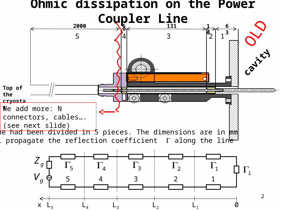
The line had been divided in 5 pieces. The dimensions are in mmWe will propagate the reflection coefficient along the line
0x
12345L12345
gV
gZ
L1L2L3L4L5
2
cavit
y
Ohmic dissipation on the Power Coupler Line
We add more: N connectors, cables…. (see next slide)
OLD

Probably not yet the final configuration but very close to the final one
3
Ohmic dissipation on the Power Coupler Line
0x
123410L123410
gV
gZ
L1L2L3L4L10
cavit
y
Top of the cryostat
5
6
7
8
9
10
50
N connectors
900
25
25
50
1000
Thermal shielding
coupler
Thermal shield
Th
erm
al s
hie
ld
NEW
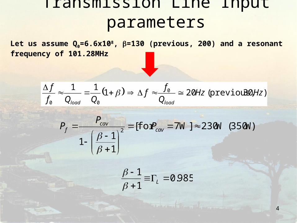
Transmission Line Input parameters
W)350(W230]W7for [
11
12
cavcav
f PP
P
985.01
1
L
Let us assume Q0=6.6x10⁸, =130 (previous, 200) and a resonant frequency of 101.28MHz
)30 previous,(20111 0
00
HzHzQ
ff
QQf
f
loadload
4
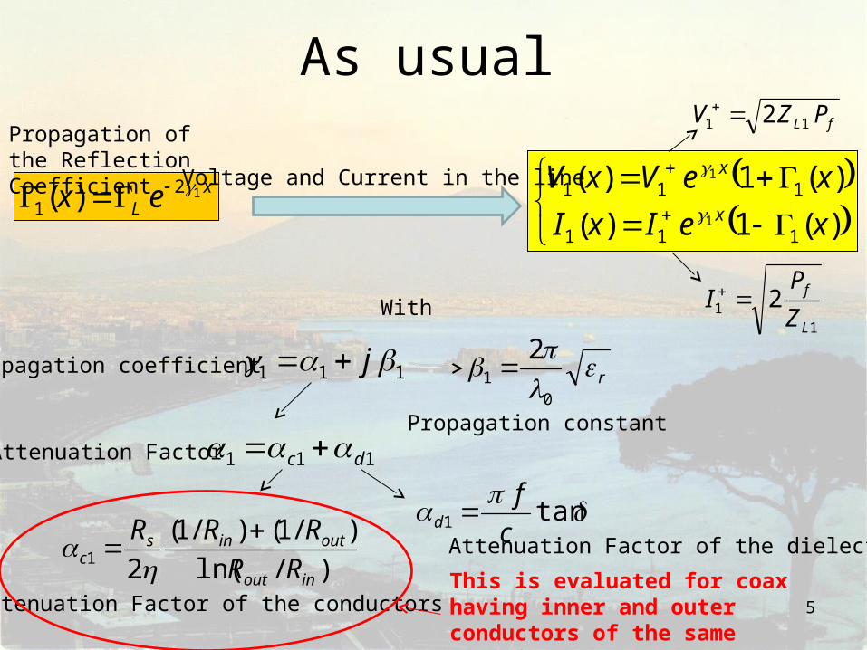
As usual
xL ex 12
1 )(
)(1)(
)(1)(
111
111
1
1
xeIxI
xeVxVx
x
With
111 j
111 dc
)/ln(
)/1()/1(
21inout
outinsc RR
RRR
tan1 c
fd
r0
1
2
fL PZV 11 2
11 2
L
f
Z
PI
Propagation of the Reflection Coefficient
Voltage and Current in the line
Propagation coefficient
Attenuation Factor
Attenuation Factor of the conductors
Attenuation Factor of the dielectrics
Propagation constant
5
This is evaluated for coax having inner and outer conductors of the same material
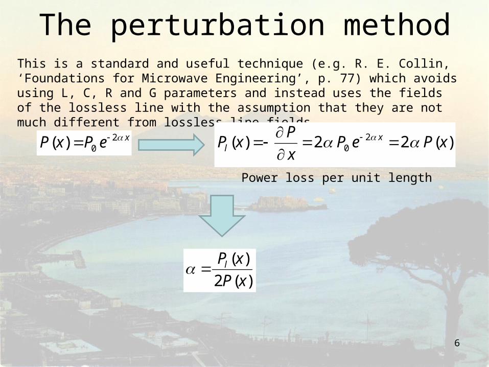
The perturbation method
6
This is a standard and useful technique (e.g. R. E. Collin, ‘Foundations for Microwave Engineering’, p. 77) which avoids using L, C, R and G parameters and instead uses the fields of the lossless line with the assumption that they are not much different from lossless line fields
xePxP 20)(
Power loss per unit length
)(22)( 20 xPeP
x
PxP x
l
)(2
)(
xP
xPl

New alfa
7
The fields of a TEM mode propagating trough the coax in cylindrical coordinates are the following:
aB
iE ρ
ˆ2
ˆ)/(ln
0
0
0
xj
xj
eZ
V
eab
V
0
2
0*
2)(
2
1)(
Z
VdSxP
S
HE With the surface S defined as (ab)
and (0 2)
b
R
a
R
Z
VldSH
RdSH
RxP sosi
S
toso
S
tisi
l
oi
20
2
022
4/
22)(
b
R
a
R
ZxP
xP sosil
04
1
)(2
)(
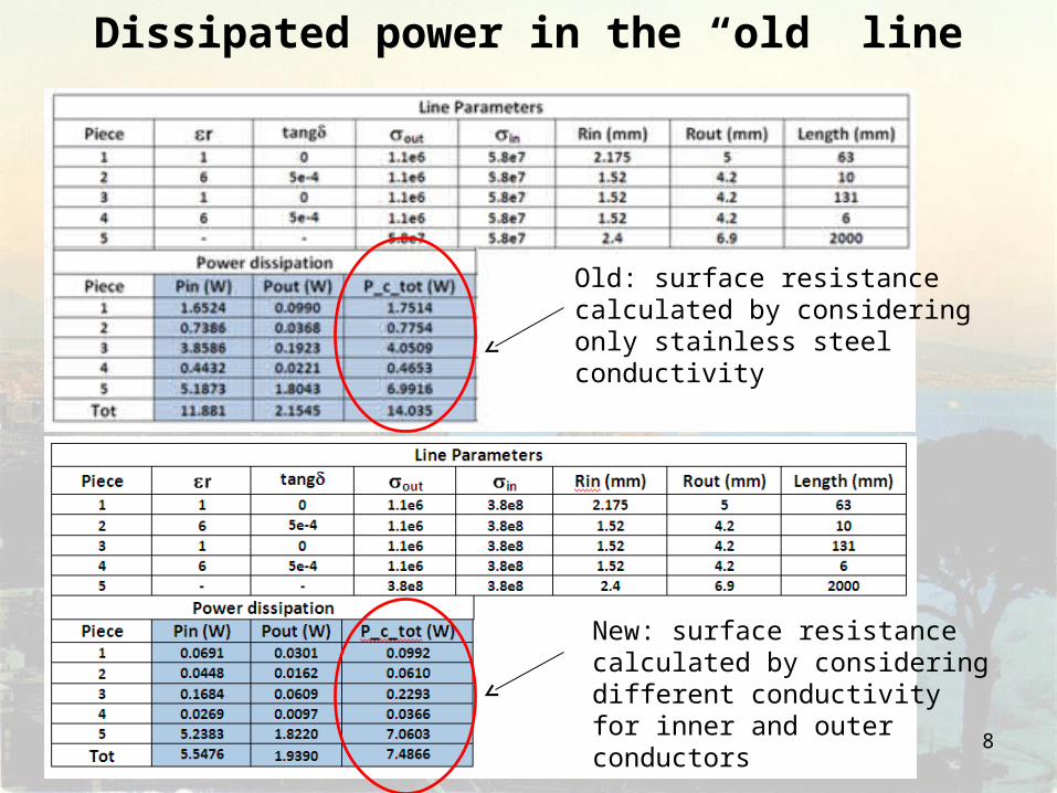
Dissipated power in the “old” line
8
Old: surface resistance calculated by considering only stainless steel conductivity
New: surface resistance calculated by considering different conductivity for inner and outer conductors

Results new line
9
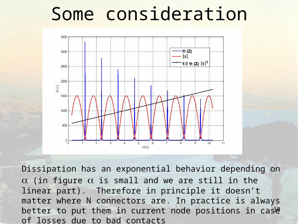
Some consideration
10
Dissipation has an exponential behavior depending on (in figure is small and we are still in the linear part). Therefore in principle it doesn’t matter where N connectors are. In practice is always better to put them in current node positions in case of losses due to bad contacts
Comments• Total power dissipation is compatible with the
one in TRIUMF• Final values for each part of the line may
change after thermal analysis• We know values of the dissipation factor of
the cables and connectors only at room temperature
• Possible cryogenic tests of cables and N connectors (in Liquid Nitrogen) to measure the behaviour of the attenuation at low temperatures... If really needed
11

Radiation Pressure
• We don’t care about microphonic excitation as we work in CW
• We don’t care about Lorentz detuning as the symmetry of our structure and the thickness of the copper layer exhibit a quite safety margin
• We care about additional forces on tuner plate (more expensive moving engine to buy!!)
12
Radiation Pressure
13
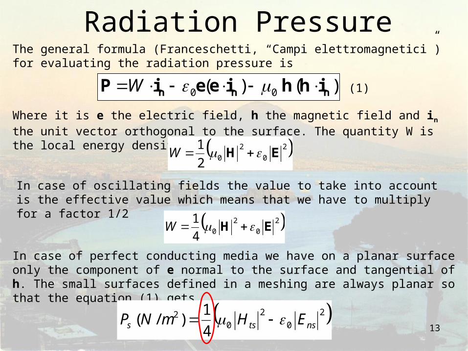
The general formula (Franceschetti, “Campi elettromagnetici”) for evaluating the radiation pressure is
)()( 00 nnn ihhieeiP W
Where it is e the electric field, h the magnetic field and in the unit vector orthogonal to the surface. The quantity W is the local energy density
2
0
2
02
1EH W
In case of oscillating fields the value to take into account is the effective value which means that we have to multiply for a factor 1/2
2
0
2
04
1EH W
In case of perfect conducting media we have on a planar surface only the component of e normal to the surface and tangential of h. The small surfaces defined in a meshing are always planar so that the equation (1) gets
(1)
2
0
2
02
4
1)/( nstss EHmNP
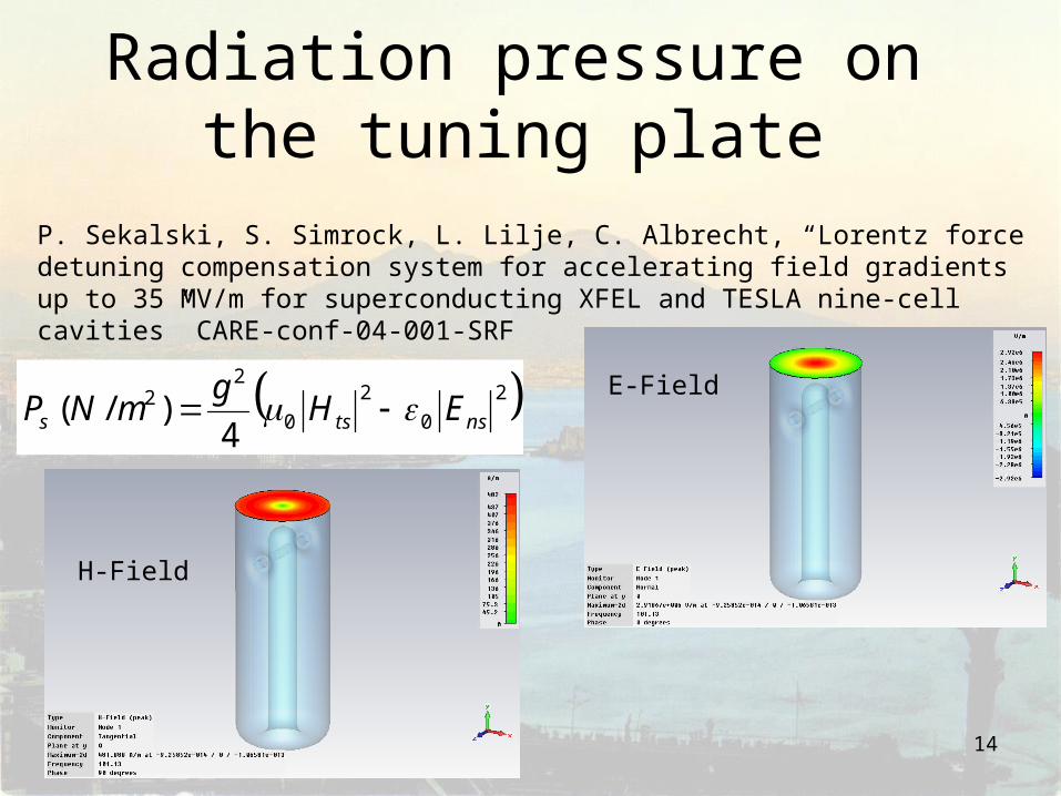
Radiation pressure on the tuning plate
14
P. Sekalski, S. Simrock, L. Lilje, C. Albrecht, “Lorentz force detuning compensation system for accelerating field gradients up to 35 MV/m for superconducting XFEL and TESLA nine-cell cavities” CARE-conf-04-001-SRF
2
0
2
0
22
4)/( nstss EH
gmNP
E-Field
H-Field
15
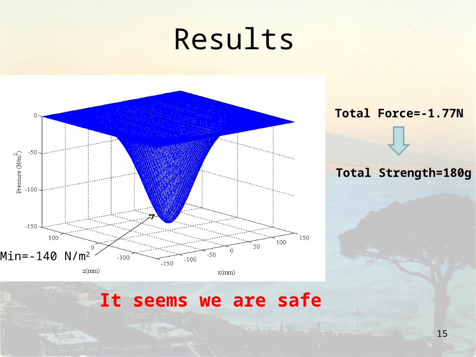
Results
Min=-140 N/m2
Total Force=-1.77N
Total Strength=180g
It seems we are safe
CLIC• Walter Wuensch would like to have from me as soon
as possible (less then 1 month) a document containing what we intend to realize by pointing out the first practical steps.
• He also agrees on the possibility of having someone (namely Vasim...) here at CERN for a while in order to make easier the exchange of information, but this is a future step at the moment.
• I’ve spoken with Vasim on Tuesday asking for some info and especially for any kind of material in order to have a more detailed overview of the structure
• I discussed also with Riccardo Zennaro and he would like to have the matrix of circuit model and also all the possible HFSS or whatever files of the structure
16


