When incentives backfire: Spillover effects in food choice

Manuela Angelucci∗, Silvia Prina†, Heather Royer‡, Anya Samek§. ¶

September 30, 2016

Abstract

Little is known about how peers influence the impact of incentives. We investigate two

mechanisms by which these effects can occur: through peers’ actions and peers’ incentives. In

a field experiment on snack choice in the school lunchroom (choice of grapes versus cookies),

we randomize who receives incentives, the fraction of peers incentivized, and whether or not

it can be observed that peers’ choices are incentivized. We show that, while peers’ actions

– picking grapes – have a positive spillover effect on children’s take-up of grapes, seeing

that peers are incentivized to pick grapes has a negative spillover effect on take-up. When

incentivized choices are public, incentivizing all children to pick grapes has no statistically

significant effect on take-up, as the negative spillover offsets the positive impacts of incentives

on take-up.

Keywords: food choice, incentives, spillovers, field experiment

JEL Classification: C93, I1, J13

∗University of Michigan (mangeluc@umich.edu)†Case Western Reserve University (silvia.prina@case.edu)‡University of California Santa Barbara and NBER (heather.royer@ucsb.edu)§University of Southern California (AnyaSamek@gmail.com)¶We are grateful to Tristin Ganter, Justin Holz, and the rest of the Behavioral and Experimental Economics

(BEE) Research Group at the University of Chicago for conducting the experiment, to Meera Mahadevan andIrvin Rojas for their outstanding research assistance, and to Michele Belot, Marianne Bitler, Kitt Carpenter,David Chan, Silke Forbes, Peter Kuhn, Pedro Rey Biel, Scott Shane and seminar participants at the NBERSummer Institute, University of Michigan, University of Chicago Harris School, Universidad Pompeu Fabra,Bocconi University, and the World Bank for their comments.

1

1 Introduction

Incentives are a cornerstone of economics. As such, their use is frequent in many domains,

including education, health, pro-social behavior, and the labor market.1 While often being

successful at improving behaviors or outcomes, incentives can backfire. This is because incentives

can act as both prices and signals. While the price effect of a higher incentive increases take-up,

the signaling effect may increase or decrease take-up.

For example, incentives can signal about the difficulty of the task (Benabou & Tirole, 2003)

or the quality of the good incentivized (e.g., Nelson (1970); Shapiro (1983); Milgrom & Roberts

(1986)), may make a subject feel controlled (deCharms, 1968) or, more broadly, convey “bad

news” (Gneezy et al. , 2011). Consistent with this signaling theory, Gneezy & Rustichini (2000)

find in two separate experiments that performance on a task falls when small monetary incentives

are offered, compared to offering no incentives. Fischer et al. (2014) find that the subsequent

demand for various products decreases with their introductory price.2

A limitation of the literature on the signalling effects of incentives is that it focuses on the

effects of incentives on their recipients (the direct effects), neglecting the spillover effects of

incentives.3 For example, consider paying students to choose a healthy snack at school. The

direct effect of the incentive program, absent the influence of peers, may result in students

eating more of the healthy snack. At the same time, these incentives can cause two types of

spillover effects. One spillover effect operates through observing peers’ actions and a second

works through observing peers’ incentives. If I see my friends pick the healthy snack, I may

think that this snack is delicious and healthy. However, if I see my friends incentivized to

choose this snack, I may think that it is not tasty (and thus, why it was incentivized). These

two spillover effects are not necessarily of the same sign or size nor are they constant, as their

magnitudes may vary with how many of my friends are incentivized.

In sum, when we observe that incentivizing children’s choice of a healthy snack affects their

eating behavior, we are observing a combination of (i) the direct effect of incentives – paying

a child to pick a healthy snack, (ii) the effect of peers’ action – changing peers’ choice of the

1A not nearly-exhaustive list of these studies include Volpp et al. (2008, 2009); Charness & Gneezy (2009);Acland & Levy (2015); Babcock & Hartman (2010); Babcock et al. (2015); Cawley & Price (2013); John et al.(2011); Royer et al. (2015); Belot et al. (2013); List & Samek (2014, 2015); Loewenstein et al. (2016) forhealthy behaviors, Angrist et al. (2009); Bettinger (2012); Fryer Jr (2011); Levitt et al. (2011b,a) for academicachievement, Ariely et al. (2009); Lacetera & Macis (2010); Lacetera et al. (2013) for pro-social behavior, andGneezy & List (2006); Fehr & List (2004); Bandiera et al. (2013); Shearer (2004) for worker effort.

2See Deci et al. (1999) for a meta analysis of the signaling effects of incentives from psychology and Gneezyet al. (2011) and Kamenica (2012) for evidence from economics.

3Following the taxonomy of Angelucci & Di Maro (2016), we define spillover effects in this paper as peer socialinteraction effects.

2

healthy snack, and (iii) the effect of peers’ incentives – watching that peers are incentivized

to pick the healthy snack. Moreover, three implications of considering the signalling effects of

incentives are 1) these spillover effects are of indeterminate sign, 2) the overall effect (i.e., the

sum of the direct and spillover effects) may differ from the direct effect, and 3) the overall effect

may vary with the fraction of peers incentivized, if each spillover effect is non-linear with respect

to the fraction incentivized.

The goal of this paper is to study the impact of incentives through peers’ actions and peers’

incentive status and, specifically, to test whether spillover effects can undo the direct effect of

incentives. To do that, we design and conduct a field experiment that lets us measure the total

effect of incentives and decompose it into its direct effect and its spillover effects. We offer grapes

and cookies and incentivize the choice of grapes versus cookies of 1,600 children in grades K-8 in

a low-income Chicago neighborhood. Almost a third of US children aged 2-19 are now deemed

overweight or obese, and part of the problem is the habitual decision to consume high calorie,

low nutrient foods (Ogden et al. , 2010). Thus, incentivizing the choice of healthy food may be

one policy tool to reduce the rates of overweight and obesity.

This experiment is uniquely designed to both measure the total effect of incentives and

decompose this total effect into the direct effect of incentives and the spillover effects of incentives

that occur through peers’ action and incentives. To do so, the experiment has two stages. In

stage 1, children choose grapes or a cookie simultaneously, without observing their peers’ choices.

We define their peers in this case as other children sitting at their lunch room table. In stage

2, we allow children to switch their snack of choice after observing peers’ initial choices and, in

some cases, peers’ incentive status. We call the stage 1 decision the direct effect of incentives,

because this choice is unaffected by peers’ actions and incentive status, unlike the choice in stage

2, which encompasses direct and spillover effects.

To identify the direct effect of incentives, we randomize who is incentivized to choose grapes.

To separate the spillover effects of peers’ actions from the spillover effects of peers’ incentive

status, we randomize both the fraction incentivized at each table and whether a student’s choice

of incentivized grapes is public knowledge (our public treatment). Randomizing the fraction of

tablemates incentivized allows us to identify the spillover effects under weaker assumptions than

much of the prior literature.4

4As summarized by Baird et al. (2014), the previous literature identifies spillover effects by not treating somegroup members (e.g., Angelucci & De Giorgi (2009); Barrera-Osorio et al. (2011); Bobonis & Finan (2009); Duflo& Saez (2003); Lalive & Cattaneo (2009); Guiteras et al. (2015)), by using plausible exogenous variation in thefractions of peers treated (e.g., Babcock & Hartman (2010); Beaman (2012); Conley & Udry (2010); Duflo & Saez(2002); Munshi (2003)), and by looking at differential treatment effects within a predetermined peer group (e.g.,Banerjee et al. (2013); Chen et al. (2010); Macours & Vakis (2008); Neumark-Sztainer et al. (2012)).

3

Our main finding is that, in the public treatment, incentivizing all children has no statistically

significant effect on grape take-up relative to incentivizing no children. The direct effect of

incentives is positive - meaning that take-up of grapes is initially higher in the 100% incentivized

tables before observing peers’ behaviors. However, after observing that all children who chose

grapes were incentivized to do so, some children in the 100% incentivized tables switch from

grapes to cookie. This degree of switching does not occur in tables in which all children are

incentivized and incentives are private. Using the random variation in the fraction of children

incentivized (i.e., not just comparing the 0% and 100% incentivized tables), we show that there

are non-linear spillover effects of incentives with respect to the fraction incentivized in the

public treatment. The overall effect of incentives is positive when we incentivize up to two

thirds of children, while it becomes statistically indistinguishable from zero when we incentivize

all children. Conversely, the spillover effects are positive in the private treatment, in which the

incentive status of other is not visible, for all fractions of incentivized children.

Imagine that our experiment consisted of stage 1 only, that is, we randomly offered incentives

and we forced the choice to occur simultaneously. If we had done this, we would have measured

the direct effects only, and concluded that incentives have a strong positive effect on the take-

up of grapes, while, in fact, this is not always the case. Similarly, imagine that we had not

separated stages 1 and 2 and compared the final grape take-up in tables with 0 and 100% of

children incentivized. In that case, we would not have been able to separate the direct and

the spillover effects of incentives and may have concluded that our subjects do not respond to

our incentives, while, in fact, they do, but in offsetting ways. Lastly, if we had not let the

fraction of children incentivized vary across tables, we would not have been able to measure the

non-monotonicity in the spillover effects of incentives.

In sum, our experiment has shown that spillover effects can be i) large, ii) positive or negative,

depending on the relative salience of peers’ action and incentive status, and iii) big enough to

offset any positive effect of incentives.

The finding that the spillover effect of peers’ incentive status is negative is consistent with

the hypothesis that incentives are “bad news.” However, other explanations are possible. While

we rule out that the effects of peers’ incentives are driven by envy or fairness issues, by a desire

to conform differently to one’s best friends, popular kids, or kids of the same gender than to

other types of children, and by changes in the perceived value of the prizes, other explanations

may be possible.

Our findings have three broad implications. First, to understand the full impact of incentives,

one should design experiments to capture spillover effects. Ignoring the spillover effects might

4

result in imprecise policy recommendations because the direct and spillover effects could possibly

offset one another. For example, in our experiment, the direct effect of incentives can be larger

than the overall effect of incentives, when incentives are public.

Second, the presence of non-monotonicities with respect to the fraction incentivized makes

extrapolation and policy scale-up from field experiments challenging. The existence of “social

multipliers” (Glaeser et al. , 2003) is well known. However, the implicit assumption – backed by

abundant empirical evidence – is that the multiplier is monotonic and that, therefore, the direct

effect of incentives is a lower bound of its net effect (in absolute level).5 This is not the case

in our setting, since the overall effect of incentives in the public treatment is positive when we

incentivize up to around two thirds of table mates, but zero when we incentivize all subjects.

The existence of these non-linearities implies that field experiments incentivizing different

fractions of the subject pool may come to very different conclusions about the effects of the

same type of incentive. For example, consider the effect of PROGRESA’s conditional cash

transfers for human capital accumulation. These transfers were given to about 75% of the

population in treated villages, and have been shown to have positive direct and spillover effects

on school enrollment (Angelucci et al. , 2010; Bobonis & Finan, 2009; Lalive & Cattaneo, 2009).

If the spillover effects vary non-monotonically with the fraction of the treated population, the

estimated effects in the evaluation villages may differ in both sign and magnitude from the effect

at the national level, because different fractions of the population are treated after the program

is rolled out.

Third, if observing others’ incentive status reduces take-up, private incentives may be prefer-

able. This may not be feasible in most settings, as people communicate and interact.

One should be cautious in generalizing our results. Different settings or populations may

lead to different spillover effects of incentives. The main conclusion of this paper, nevertheless,

remains valid (and valuable): spillover effects can undo the direct effect of incentives. Further

research should study whether different designs and contexts deliver similar results.

This caveat notwithstanding, we believe that evaluating the spillover effects of incentives

may be worthwhile in several settings. The first type of setting is one in which the value of

the incentivized action is not well known and in which subjects believe peers and policy makers

may have private information (e.g., new technology adoption). In such settings, incentives

allow subjects to learn from peers’ and policymakers’ actions. However, as the signalling effects

of incentives can be both negative and positive, careful consideration should be made when

5Examples include the take-up of welfare (Borjas & Hilton, 1996; Bertrand et al. , 2000), employer-sponsoredhealth insurance (Sorensen, 2006), retirement plans (Duflo & Saez, 2003), public prenatal care (Aizer & Currie,2004), disability insurance (Rege et al. , 2009) and movie attendance (Moretti, 2011), among others.

5

invoking incentive schemes for public policy. For example, the Physician Payment Sunshine

Act, which requires drug manufacturers to disclose certain payments to physicians, may reduce

the demand for drugs from the paying manufacturers, if the payments are perceived to signal

that the drugs of a given manufacturer are not as effective as others. The second type of

setting is one in which the incentivized behavior has short-run costs but long-run benefits (e.g.,

nutrition, exercise, education, and other behaviors that increase health and human capital).6

In this case, the incentive may increase the salience of the short-term cost over the long-term

benefit of the incentivized action. The third type of setting is in pro-social behaviors, such as

recycling, charitable giving, or blood donation, whose ‘warm-glow’ value exceeds the monetary

value of incentives (see, e.g., Frey & Oberholzer-Gee (1997)). Finally, the fourth possible setting

is in interesting or pleasant activities, where incentives may reduce interest in the task.7

2 Theory

Before discussing the experiment, we present a simple model to demonstrate that positive and

negative direct and spillover effects of incentives can plausibly exist, in the spirit of Benabou

& Tirole (2003). Benabou & Tirole (2003) model the behavior of a principal, who has private

information on the attributes of an action (e.g., how pleasant or difficult it is), and an agent, who

is uncertain about the net benefit of undertaking the action and who is aware of this asymmetric

information. The principal incentivizes the action in a way related to its cost for the agent. The

agent is affected by the incentive in two opposite ways: the incentive increases the benefit of

undertaking the action; however, it also provides the agent with a signal about the cost of

undertaking the action. Since high incentives may signal a costly action, principals uncertain

about the signaling effect of the incentive may set incentives that reduce the likelihood that the

agent will undertake the action, as they increase the benefit from undertaking the action less

than they increase its cost.

We extend this model to consider how, in addition to these direct effects of incentives,

incentivizing an action affects the agent’s behavior also by changing the actions and incentive

status of the agent’s peers (Banerjee, 1992).

Consider the choice of grapes, Gi = 1, versus cookies, Gi = 0, for child i in a setting with

asymmetric information. The child decides to pick grapes over cookies if the expected private

6Gneezy et al. (2011) review the evidence of incentives backfiring in this type of setting.7Kamenica (2012) review the evidence of incentives backfiring for the last two settings.

6

benefits of this choice, Bi, exceed its costs, C:

E[U(Gi = 1)− U(Gi = 0)] = Bi − C. (1)

The monetary (or cash-equivalent) cost of choosing grapes over cookies, C, is a function of

incentives, I. The child’s beliefs of the benefits, Bi, depend on her idiosyncratic taste, τi, as well

as on the behavior of her peers and of the experimenter, whom the child believes to have private

information about the relative value of grapes over cookies, such as their relative health benefits

and taste. The child observes the behavior of her peers and of the experimenter to infer their

private information. This setting does not require the experimenter and peers to have more or

better information than the child. However, it does require that the private information of the

experimenter and peers be complementary to the child’s information, so that observing peers’

actions and incentives can lead to changes in the child’s belief. For example, in our empirical

setting, cookies are not typically part of the lunch menu, so some children may not know how

good the offered cookies taste. Moreover, the experimenter may have seen other children make

this choice before, and, therefore, be expected to have information about children’s relative

preferences over the snacks.

In our setting, the experimenter announces that an unspecified fraction of children will be

incentivized to pick grapes, as is often the case in public policy settings. This announcement

affects the child’s beliefs of the benefits, Bi. Then, the child observes whether she is incentivized

to pick grapes, I, which also affects her beliefs of Bi, and makes an initial snack choice simulta-

neously with her peers. At this point, she can see the fraction of her peers who choose grapes

over cookies, G−i, and, in some cases, also the fraction of her peers who choose incentivized

grapes, I−i. I−i is a lower bound of the fraction of peers who were incentivized to choose grapes,

TP . This additional information may lead her to revise her initial beliefs, and, subsequently,

her snack choice. In sum, the expected utility of choosing grapes over cookies can be expressed

as:

E[U(Gi = 1)− U(Gi = 0)] = Bi(τi, G−i(TP ), I−i(TP ), I)− C(I) (2)

The main goal of our experiment, which we detail later, is to distinguish (i) the direct and

spillover effects of incentives and (ii) spillover behavior due to responses to the fraction of peers

who choose grapes (i.e., spillover effects due to peers’ choices) versus responses due to the fraction

choosing incentivized grapes (i.e., spillover effects due to peers’ incentive status). We do that

by randomly varying whether each child is incentivized, how many of her peers are incentivized,

7

and whether the incentive status of some of her peers are visible or not. Conversely, we cannot

identify the effect of announcing that some children are incentivized because this announcement

is made to all.

2.1 Direct Effect of Incentives

Consider first the direct effect of incentives, I, on the incentivized person:

∂E[U(Gi = 1)− U(Gi = 0)]

∂I=∂Bi∂I− ∂C

∂I(3)

The first right-hand side term, ∂Bi∂I , is the effect of introducing (or increasing) the incentive

on the child’s belief on the relative value of grapes over cookies. The sign of this effect is

indeterminate. For example, in Benabou & Tirole (2003), being incentivized (or having a higher-

valued incentive) signals “bad news” – e.g., that the experimenter and the other children perceive

grapes to be unpopular or unpleasant.8 This may make her revise her prior beliefs about the

benefits of grapes downward. On the other hand, the incentive may signal that the experimenter

thinks grapes are really good for the child (maybe despite not tasting as good as the cookie),

inducing her to revise her prior belief of the benefits of grapes upward.9

Conversely, the second right-hand side term, ∂C∂I , which represents the effect of the incentives

on cost, is negative, as compensating the child to pick grapes over cookies reduces its cost. In

sum, the sign of the direct effect is unknown, due to the ambiguity of the sign of ∂Bi∂I .

2.2 Spillover Effects of Incentives

Now consider the effect of the fraction incentivized. This is what we call the spillover effect. To

do that, consider an increase in the proportion of children who are incentivized to pick grapes,

TP , which affects the fraction of her peers who initially choose grapes over cookies, G−i, and

who initially choose incentivized grapes, I−i.

∂E[U(Gi = 1)− U(Gi = 0)]

∂TP=

∂Bi∂G−i

∂G−i∂TP

+∂Bi∂I−i

∂I−i∂TP

(4)

The first right-hand side term, ∂Bi∂G−i

∂G−i∂TP , is the spillover effect of incentives arising from watching

others pick grapes and has an indeterminate sign. The sign of ∂Bi∂G−i

is positive, if an increase

8In Benabou & Tirole (2003), a principal has private information about attractiveness of an action and mayoffer larger incentives for less attractive tasks. The agent, therefore, expects larger incentives to signal moreunpleasant tasks and may be less motivated to do it.

9Announcing that there will be incentives has the same ambiguous effect on beliefs. We do not discuss itfurther because, since all children receive this announcement, this effect cancels out in our empirical analysis.

8

in the proportion picking grapes sends a positive signal about the value of grapes.10 Therefore,

the sign of this first term depends on how increasing the proportion incentivized affects the

proportion picking grapes initially, ∂G−i∂TP . This has the same sign as the direct effect of incentives.

The second right-hand side term, ∂Bi∂I−i

∂I−i∂TP , is the spillover effect of incentives through watch-

ing others pick incentivized grapes. It has an indeterminate sign because the signs of its two

parts are both indeterminate. The sign of ∂Bi∂I−i

depends on how children interpret the experi-

menter’s intent to incentivize children to pick grapes and, therefore, has the same sign as ∂Bi∂I .

∂I−i∂TP has the same sign as the direct effect. Overall, taking into account the spillover effects and

their possible signs (detailed below), the sign of the overall effect of incentives can be ambiguous.

There are, therefore, the following 3 cases, also summarized in Table 1:

Case 1: Incentives send a weakly positive signal on the value of grapes (∂Bi∂I ≥ 0). When

this happens, the direct effect of incentives is positive, as ∂Bi∂I −

∂C(I)∂I > 0. If the direct effect is

positive, then increasing the proportion incentivized increases the proportion choosing grapes,

incentivized or not, (∂G−i∂TP > 0 and ∂I−i∂TP > 0). Moreover, if the incentive sends a weakly positive

signal on value of grapes, then the belief of the value of grapes grows with the proportion

of children choosing incentivized grapes, ∂Bi∂I−i

≥ 0, and, therefore, the two spillover effects of

incentives are also positive. That is, in this case the spillover effects through peers’ actions and

incentive status reinforce the direct effects.

Case 2: Incentives send a negative signal on the value of grapes (∂Bi∂I < 0), but the direct

effect is positive, because the cost reduction more than offsets the negative signal for incentivized

children, ∂Bi∂I > ∂C(I)

∂I . If the incentive sends a negative signal on the value of grapes, the

belief of the value of grapes decreases with the proportion of children choosing incentivized

grapes, ∂Bi∂I−i

< 0. Moreover, if the direct effect is positive, increasing the proportion incentivized

increases the proportion choosing grapes, incentivized or not, (∂G−i∂TP > 0 and ∂I−i∂TP > 0). It

follows that the sign of the spillover effect is indeterminate: the first term is positive, the second

negative. That is, in this case the spillover effects may either reinforce or offset the direct effects.

Case 3: Incentives send a negative signal on the value of grapes (∂Bi∂I < 0) and the direct

effect is negative, because the cost reduction is offset by the negative signal for incentivized

children, ∂Bi∂I < ∂C(I)

∂I . If the incentive sends a negative signal on the value of grapes, the belief

of the value of grapes decreases with the proportion of children choosing incentivized grapes,

∂Bi∂I−i

< 0. Moreover, if the direct effect is negative, then increasing the proportion incentivized

10The sign of ∂Bi∂G−i

can also be negative. We do not explicitly model this option because it would increase the

number of possible cases, and thus lengthen the exposition, without adding to our main point that the direct andspillover effects may have opposite signs. Moreover, the sign of ∂Bi

∂G−iis positive in our data, so modelling this

option is not essential in this application.

9

reduces the proportion choosing grapes, incentivized or not, (∂G−i∂TP < 0 and ∂I−i∂TP < 0). It follows

that the sign of the spillover effects is indeterminate: the first term is negative, the second

positive. That is, in this case the spillover effects may either reinforce or offset the direct effects.

In sum, we have 3 broad conclusions. First, incentives may have both a positive and a

negative direct effect.11 Second, when incentives are “bad news” (∂Bi∂I < 0), the spillover effects

of incentives can have both a positive and negative component. Third, when incentives are “bad

news,” the direct and spillover effects of incentives may offset each other. Therefore, the direct

effect may be a poor approximation of the overall effect of incentives.

Alternative models. There are multiple models that generate direct and spillover effects of

incentives of opposite signs and thus, lead to an overall effect of incentives of indeterminate

sign. For example, a model with symmetric information but with a short term cost and a long

term benefit of choosing grapes over cookies would generate similar predictions, if the public

incentives make the short term cost more prominent and hence reduce the likelihood of choosing

grapes. This would change the mechanisms behind our findings, but not our empirical setup.

Moreover, regardless of whether information is asymmetric or not, incentive salience may affect

behavior. In an environment in which incentives signal “bad news” or emphasize the short term

cost of an action over its long benefits, making incentives more prominent may increase the

perceived cost of an action, thus reducing its take-up. Lastly, a model in which there is both

an intrinsic dislike for incentives, as, e.g., they make subjects feel controlled (deCharms, 1968)

or cause envy or fairness issues (Sherif, 1937; Asch, 1958; Feldman & Kirman, 1974; Fehr &

Schmidt, 1999; Goeree & Yariv, 2014; Haun et al. , 2014) and social conformity to peers’ actions

would have the same set of predictions. Section 9 considers alternative models of behaviors -

social conformity, fairness, and envy. Support for these models is limited in our data, but others

may be possible. The goal of this paper is not to identify the exact behavior generating these

effects, but to show theoretically and empirically that these effects can exist.

3 Background and Experimental Design

To measure the direct and spillover effects of incentives, we designed an artefactual field exper-

iment (Harrison & List, 2004) in which we offer grapes and cookies to children and randomly

offer incentives to choose grapes.12 This experiment took place in school cafeterias during lunch.

Nine elementary schools in Chicago Heights, Illinois participated. Lunch is administered in much

11In empirical settings such as ours, we cannot separately identify the positive and negative direct effects ofincentive, as we observe only their sum.

12Grapes, but not cookies, are sometimes served at lunch.

10

the same way in each of these schools. Depending on their size, schools hold either 2, 3 or 4

lunch periods each day, assigning kids to periods based on their school grade. Children arrive

for lunch during their designated lunch period together with their class. They go through a

lunch line where they receive a school lunch and then sit at a table in the cafeteria. Except

for kindergartners, students can typically sit with any other children from their grade and tend

to form groups of 3-10 students at each table. In this school district, children do not have a

choice about their lunch. Moreover, Chicago Heights, Illinois is in a low-income neighborhood

and most children qualify for free or reduced-price lunch, meaning that all kids eat the same

school-provided meal each day. We are not aware of specific programs at these schools promoting

healthy eating habits.

We conducted the experiment after children had collected their lunch trays and sat down

to eat at their table, as they normally do. Once children chose where to sit, members of the

research team came to the table and read a script, reported in Appendix A, which described

the procedures of the experiment. We treated adjacent tables simultaneously. This, and the

fact that children are required to stay seated at their table throughout the entire lunch period,

minimized cross-table contamination. To ensure compliance, we assigned one research assistant

to one table at a time and ensured that adjacent tables could not easily see what was happening

at nearby tables.

Each child was asked to pick both a grape card (green on the back) and a cookie card (blue

on the back) from a card deck (see Figure 1). To facilitate data collection, each child’s ID

number from the experiment was written on each of his or her cards. Then, each child made

a choice: he or she could either choose to have grapes as an additional food (by placing the

grape/green card down on the table), or he or she could choose to have cookies as an additional

food (by placing the cookie/blue card down on the table). Children were told that they could

choose only one snack, and that the actual food item they had selected would be delivered

to their table immediately at the end of the experiment. The initial choice was always made

simultaneously and children were asked not to talk during the experiment. Children complied

with these requirements. After the initial choice, children had twenty seconds to play a different

card after having observed their peers’ choices.

We randomized 1) which child received an incentive to choose grapes, 2) the fraction of

each lunch table that received an incentive to select grapes, and 3) in which tables choosing

incentivized grapes are visible by peers (public treatment) or not (private treatment). In par-

ticular, for each table, we had a stack of cards, which had either 0, 50, or 100% of cards with

incentives. At tables with 50% of cards incentivized, because the incentivized cards where ran-

11

domly stacked in the decks and the number of occupants changes by table, the actual fraction

of children receiving incentives varies between 11 and 80 percent. This variation is seen in Table

2.

In all treatments, children were alerted to the possibility that they may be eligible for a

prize depending on the card they draw, and a poster with all possible prizes was displayed to

the kids. The value of each prize was roughly 50 cents. The prizes included glow-in-the-dark

bouncy balls, small trophies, and bracelets and pens of different types.

If students were eligible for an incentive, their grape card depicted a small gold token. For

the 50 percent incentive treatment, the cards came from a deck where 50 percent of the grape

cards portrayed a gold token. In the 100 percent incentives treatment, all the grapes cards

depicted the coin.

In the private treatment, children play their cards face down, so that children can observe

only the color of the card, but not the presence or absence of the incentives. In the public

treatment, on the other hand, children play their cards face up, so that anyone at the table can

observe whether the chosen grapes are incentivized or not.

With the three levels of randomization, we can divide children into six table types, depending

on (i) whether 0, 50, or 100% of the cards for a table is incentivized, and (ii) whether the

incentivized choices are public or private. If we further group children depending on their

incentive status, we end up with eight groups:

• Private-0-no incentive: Children in the Private treatment in which none of the grape cards

were incentivized.

• Public-0-no incentive: Children in the Public treatment in which none of the grape cards

were incentivized.

• Private-50-no incentive: Children in the Private treatment in which 50% of the grape cards

were incentivized but the child’s own card was not incentivized.

• Public-50-no incentive: Children in the Public treatment in which 50% of the grape cards

were incentivized and the child’s own card was not incentivized.

• Private-50-incentive: Children in the Private treatment in which 50% of the grape cards

were incentivized and the child’s own card was incentivized.

• Public-50-incentive: Children in the Public treatment in which 50% of the grape cards

were incentivized and the child’s own card was incentivized.

12

• Private-100-incentive: Children in the Private treatment in which all of the grape cards

were incentivized.

• Public-100-incentive: Children in the Public treatment in which all of the grape cards were

incentivized.

We designed the experiment by randomizing each school-by-period table in such a way as to

have one quarter of the school-by-period tables assigned to the 0% and 100% treatments each,

and the remaining half to the the 50% treatment, cross randomizing the public and private

treatment to have half of the school-by-period tables in each group.

We record both the initial food choice, G1, and the final food choice, G2. We use G1 to

measure the direct effect of incentives because this choice occurs simultaneously and before

children can observe their peers’ choices and incentives. We use G2 to measure the spillover

effect of incentives because this final choice occurs after having observed peers’ choices and

incentives.

Our experimental design makes advances in the peer effects literature along 4 dimensions.

First, by recording both initial and final snack choice, we can both measure the overall effect

of incentives and decompose it into the direct and the spillover effects of incentives. The ex-

isting literature typically focuses on measuring either the overall effects, without being able to

decompose them (as in, e.g., Royer et al. (2015)) or the direct effect only, without being able

to study how incentives would affect behavior once spillover effects are allowed to operate (as

in, e.g., Just & Price (2013)).

Second, by randomly varying the fraction of treated peers and allowing people to switch

snack after observing their peers’ actions and incentives, we can measure spillover effects on

both incentivized and non-incentivized subjects. In many papers that measure spillover effects,

this is not possible unless one is willing to make (potentially unrealistic) assumptions. This

occurs because papers that measure spillover effects typically do so by looking at the effect of

a treatment on untreated subjects. If treated and untreated subjects are randomly selected

(as in, e.g., Duflo & Saez (2003)), the spillover effects on the treated can be identified from

the untreated under the assumption that these effects are additive, but such an assumption

is not necessarily backed by any theory. If treated and untreated subjects are not randomly

selected (as in, e.g., Angelucci & De Giorgi (2009)), then the spillover effects on the treated can

be identified from the untreated under the additional and less realistic assumption that these

effects are homogeneous across different types of subjects.

Third, by randomly varying the fraction of treated peers, we can measure potential non-

13

linearities in spillover effects. In many papers that measure spillover effects, this variation is not

random. For example, in Babcock & Hartman (2010), some subjects have more treated friends

than others. However, these subjects may also have more friends to begin with, so the variation

in treated friends is not exogenous. Therefore, while these papers can measure the combined

effects of treating different subjects and having different numbers of treated peers, we can isolate

the latter effect under weak identification assumptions.

Fourth, by having private and public treatments, we can separate the spillover effect of peers’

actions (observed both in the private and public treatment) from the spillover effects of peers’

incentives (observed in the public treatment only). To our knowledge, this is the first time such

a decomposition has been done.

4 The data

4.1 Sample

A total of 1,771 children participated in the experiment. We drop 14 tables of 10 from the main

analysis because we do not believe that kids can see all others’ decisions at such a large table.

The results in the next section are qualitatively unchanged if we include tables with 10 children.

We complemented the experimental data with a short survey assessing the social networks

of kids (available upon request). The survey included questions asking children to name up to

5 of their friends. There were also questions about each child’s perceived social status relative

to other children and the most popular kid boy and girl in their class. A total of 1,286 (73%)

children filled out the questionnaire.

After dropping large tables, our final sample consists of 1,631 children, of whom 1,187 com-

pleted the questionnaire, sitting at 270 school-by-period tables.13

The final size of each of the 8 groups varies because some of the tables in the cafeteria were

empty.

4.2 Descriptives, balance tests, and food choice

Table 3 shows the mean and standard deviations of several socioeconomic variables for each of

the eight groups. Lunch tables have on average 6.45 children of which 47 percent are boys. The

average grade is fourth grade, 39% of children at each table are African American and 52% are

Hispanic, and 87% of the children at each table are on the free lunch program (and some more

13Non-participation in the survey is also due to a number of reasons: either children were too young, or teachersoverseeing the lunch period asked us not to administer the survey, or not enough time was available for all childrento complete the survey.

14

qualify for lunch at a reduced price). We test that the variables are balanced across groups in

the lower panel of Table 3, which shows the F-test of joint significance of the 8 group dummies,

when regressed on each of these variables together with school-by-period strata. None of the

F-tests are significant at conventional levels, consistent with random assignment.

We also check for balance using the actual fraction of student incentivized as opposed to

these discrete groups considered in Table 3. Recall, while the grape cards for the 50% incen-

tivized tables were drawn from a deck where half of the cards were incentivized, the actual

fraction incentivized deviated from 50%. We regress the proportion of children incentivized at

each table on table size and children’s age, gender, race, grade, and school lunch status (free,

reduced, or none), as well as on school-by-period strata. The F-test of joint significance of the

coefficients of the socioeconomic variables has a p-value of 0.087. This is driven by a smaller

table proportion incentivized for third and six graders by chance. Once we exclude grade, the

F-test of joint significance of the coefficients of the remaining socioeconomic variables has a p-

value of 0.543. For this purpose, and to improve the precision of the estimates, we control for all

the aforementioned variables in all our specifications. The results are qualitatively unchanged

whether we add these variables or not.

5 Total effect of incentives

Our goal is to estimate the total effect of incentives on grape take-up and to decompose this

total effect into the direct effect of incentives and the spillover effects due to peers’ actions

and incentives. To do that, we first consider the effect on final grape take-up, the variable G2,

which is the sum of the initial grape choice, G1, and the revised choice, ∆G. We then proceed

to estimate the direct effects of incentives using the variable G1 and the spillover effects of

incentives using the variable ∆G. We show how these variables change differently in the private

and public treatments as the fraction of peers incentivized varies from 0 to 100 percent.

Before analyzing the data, recall that children make their first choice, G1 based on an initial

belief of the proportion of peers incentivized. This belief does not vary systematically across the

private and public treatments because children are randomly assigned to it and, at this stage,

they all have the same information.

The initial beliefs can change after observing peers’ initial choice. Consider private tables

first, in which peers’ initial choices, but not incentive status, are observed. In these tables, peers’

choices send a mixed signal: if more peers pick grapes, it may mean they like grapes, or they

are incentivized to choose them. Conversely, in public tables the information is less noisy, as all

15

can observe whether the chosen grapes were incentivized or not. Therefore, beliefs are revised

differently in private and public tables, and the difference in information causes better belief

updating in public tables.

Consider, as an illustrative example, two six-person tables with 100 percent incentives, one

in the private treatment and one in the public one. Suppose that children expect that 50 percent

of the table is incentivized and 50 percent of the table initially chooses grapes (this proportion

need not be identical). Initially, 4 children choose grapes in both tables. In both tables, children

revise their initial belief of the proportion choosing grapes upwards. In addition, children in the

public table may revise the belief of the proportion incentivized upwards too, as they are certain

that at least two thirds of the table are incentivized, while it is not clear how the latter changes

in the private table. If the proportion picking grapes is “good news,” while the proportion being

incentivized to pick grapes is “bad news,” the public table receives more bad news than the

private table, and, therefore, we expect a smaller increase in final grape take-up in the public

table than in the private table or ∆G(100, public)−∆G(100, private) < 0.

Now consider two six-person tables with 0 percent incentives, one in the private treatment

and one in the public one. The initial beliefs are the same as before – 50 percent are incentivized

and pick grapes. However, now only two children pick grapes initially. Both tables revise the

“good news” down, as fewer than expected children pick grapes. In addition, children in the

public table revise the belief of the proportion incentivized, the “bad news” downwards too, as

they are certain that at most two thirds of the table are incentivized, while it is unclear how

this belief changes in private tables. Using the previous language, the public table now receives

less bad news than the private table and, therefore, we expect a larger increase in final grape

take-up in the public table than in the private table or ∆G(0, public)−∆G(0, private) > 0.

The evidence from our data is consistent with the above examples, as we find that ∆G(100, public)−

∆G(100, private) = −0.112 (s.e. 0.040), ∆G(0, public) − ∆G(0, private) = 0.033 (s.e. 0.049),

and the difference between the two is -0.146 (s.e. -0.064). Armed with this framework of analysis,

we can proceed to look at the whole data.

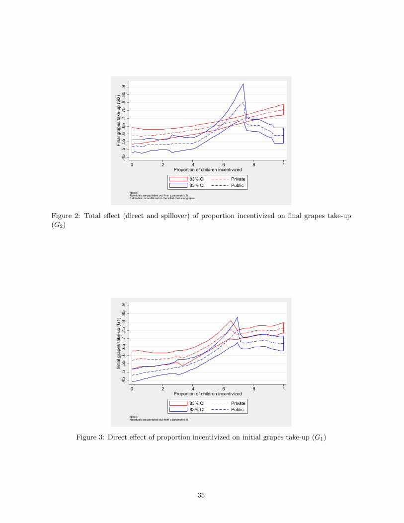
Figure 2 plots the semi-parametric total effect of table proportion incentivized on a dummy

variable indicating the final choice of grapes, G2, for the private and public treatments.14 While

14To do so, we use the Robinson’s semi-parametric estimator (Robinson, 1988) to control for the effect of thepredetermined covariates (school-by-period strata, table size, child age, gender, race, grade, and school lunchstatus) and then smooth the effect of incentive proportion on final grape choice using a local linear regressionwith a Gaussian kernel and a rule-of-thumb bandwidth. The results are robust to changes in the kernel andbandwidth, as well as to using the table, rather than the child, as the unit of analysis. We cluster the standarderrors by table. We report the 83% confidence intervals because, if the 83% confidence intervals around two pointestimates do not overlap, the parameters are statistically different from each other at the 95% level (Peyton et al., 2003). We use the same empirical approach also for the next two figures.

16

the total effect of incentives grows with the table proportion incentivized in the private treatment,

this effect is non-monotonic in the public treatment. In these tables, the total effect of incentives

grows with the proportion incentivized up until about two thirds of children are incentivized,

but it is considerably lower when all children are incentivized, to the degree to which there is

no statistically significant difference in final grapes take-up between tables with 0 and 100%

incentives. Note that, while we have few tables with 60 to 80% incentivized children (hence the

larger confidence intervals), grapes take-up among these tables differs statistically from tables

with both 0% and 100% incentivized children.15

Comparing the public and private treatments suggests that the non-monotonicity in the

public treatment is linked to the observability of incentives, as the effect is monotonic in the

private treatment. Figure 3, which measures the direct effects of incentives, confirms this because

the initial choice of grapes, made before peers’ actions and incentives are observed, grows with

the table proportion incentivized in both public and private treatments.

A comparison of Figures 2 and 3 shows evidence of no or modest spillover effects of peers’

actions and negative spillover effects of children’s incentive status. The spillover effects of peers’

actions are modest as initial and final grape choice in the private treatment are similar. The

spillover effects of children’s incentive status are negative because there is a drop from initial

to final grapes take-up where all children are incentivized in the public treatment tables (where

incentives are visible), but not in the private tables (where incentives are not visible).

Lastly, the initial choice of grapes is lower in the public than the private treatment, including

in tables where no child is incentivized, consistent with the idea that making incentives more

salient may signal “bad news” (e.g., Gneezy et al. (2011)) or make the short term costs of

picking grapes over a cookie more prominent.16

This lower initial rate of grape take-up in public tables may lead to differential effects on

belief updating. However, the sign of this effect is unclear. This is because public tables observe

both fewer peers choosing grapes (and, therefore, have fewer “good news”) and fewer peers

being incentivized to choose grapes (and, therefore, have also fewer “bad news”). We believe,

therefore, that this difference in initial grape take-up does not affect the main findings, which

follow.

To conclude, these figures provide evidence of direct and spillover effects of incentives of

opposite signs in the public treatment. The lack of a statistically significant difference in take-

15Comparing group means reinforces our main findings that the final grape take-up increases with the propor-tion of incentivized children in the private treatment but not in the public treatment.

16Children in these two arms have the same initial priors, since they know the same information, so thedifferences in initial choice cannot be driven by differences in priors.

17

up between the 0% and the 100% public tables does not mean that children in our sample

do not respond to the incentives. Incentivizing approximately 50 to 70% of children increases

final take-up by around 10-30 percentage points, but this gap shrinks and eventually is no

longer statistically different from zero when all children receive incentives. Thus, these initial

findings show that, in our experiment, public incentives backfire, but only when all children are

incentivized to pick grapes. Our next step is to decompose the total effect of incentives into its

direct effect and the spillover effects to study their sign and magnitude.

6 Direct effects of incentives

We measure the direct effect of incentives on grape choice, that is, whether receiving the in-

centives changes the recipients’ likelihood of initially choosing grapes, by comparing the initial

grape choice of incentivized and non-incentivized children. To do so, we regress child i’s initial

grape choice, G1, on a dummy variable, I, that equals 1 for children who receive incentives

and 0 otherwise. To improve the precision of the estimates, we condition on the variables X:

school-by-period strata, table size, child age, gender, race, grade, and school lunch status.

G1i = α0 + α1Ii + α2Xi + εi (5)

The coefficient α1 identifies the average treatment effect of incentives on initial grape choice.

This parameter is identified under the assumptions that (i) the variable I and the error term

ε are independent, which follows from random assignment, and that (ii) one child’s potential

outcomes are unaffected by the treatment status of others, which follows by keeping treatment

status private at this stage. We estimate the parameters of this equation by OLS, clustering

the standard errors by table. We use the same estimator, controls, and clustering for all the

regressions in this paper.

We can also interact the incentive dummy by a dummy for the public (P = 1) and private

(P = 0) treatments:

G1i = λ0 + λ1Ii + λ2Pi + λ3IiPi + λ4Xi + εi (6)

This way, we can test i) whether the direct effects of incentives are identical in the public and

private treatment (λ3 = 0) and ii) whether the initial grape choice is identical in the public and

private treatments for non-incentivized children (λ2 = 0) and incentivized children (λ2+λ3 = 0).

Column (1) of Table 4 shows the direct effects of incentives on the initial choice of incentivized

18

children (the estimate of α1 from equation (5)). Incentives increase initial grape take-up by 26

percentage points, a statistically significant increase of about 53%, compared to a 49.5% take-up

rate among non-incentivized children.

These findings are comparable in size to Just & Price (2013), who increase children’s con-

sumption of salad by 80% after offering up to $0.25 (or a lottery ticket with the same expected

value), and smaller, but consistent, with List & Samek (2014, 2015), whose incentives have a

two- to four-fold increase in the choice of healthy snacks. Conversely, our effects are larger than

the ones in Belot et al. (2013), whose piece-rate incentives to choose an extra vegetables side

dish have a small, statistically insignificant effect.

This initial choice may differ from a choice in a one-shot game that does not let them change

their mind later. However, since incentivized children are much more likely to pick grapes over

cookies, this choice nevertheless send some signal of their preferences and beliefs.

In addition, it is not clear whether children benefit from concealing their preferences. First,

each child’s outcome does not depend on the choices of others, which reduces the benefits of

strategic behavior. Second, we find that a child’s initial choice does not depend on whether

others can observe her incentive status. Recall that in the private treatment, the cards are

played face down and, therefore, one can infer other children’s choices from the color of the

card, but not whether a child was incentivized. On the other hand, for the public treatment, the

cards are played face up and the incentives can be observed. To test whether children behave

differently when they know others can observe whether or not they are incentivized, the second

row of Table 4 in column (2) provides the estimate of the difference in effect sizes in the public

and private treatment (the estimate of λ2 from equation (6)). This difference is only 0.013 and is

statistically insignificant. Moreover, in Section 9 we will show that kids’ choices are not affected

differently by the choices of their best friends, popular kids, or kids of their same gender. If

these selected peers do not especially affect a child’s behavior, it is likely that the child also

expects her behavior not to especially affect her peers.

The third and fourth rows of the tables show that the initial grape choice is 8.4 and 7.1

percentage points lower in public treatments for both non-incentivized and incentivized children

(the estimates of λ2 and λ2+λ3 from equation (6)), as we already noticed in the previous section.

7 Spillover effects of incentives

Finding positive direct effects of incentives rules out case 3 (negative direct effects of incentives)

and is compatible with both cases 1 and 2 from our theory: peers’ action (choosing grapes)

19

has a positive spillover effect on own grape take-up, while peers’ incentives (seeing peers choose

incentivized grapes) may have positive or negative spillover effects. Armed with this knowledge,

we proceed to tease out the different spillover effects from seeing other children pick grapes or

observing other children picking incentivized grapes.

Since spillovers affect the likelihood that a child may change the card played after seeing

others, our dependent variable is the difference between the final and initial grape choice, ∆G =

G2 − G1. Therefore, we begin our analysis of spillover effects by estimating how exogenously

varying the table proportion incentivized, TP ∈ [0, 1], affects ∆G:

∆Gi = β0 + β1TPi + β2TPi ∗ Pi + β3Ii + β4Pi + β5IiPi + β6Xi + εi (7)

We condition on being incentivized (I) and on the public treatment dummy (P ) because they

affect the initial grape choice, which, in turn, affects the likelihood of ending up with grapes. We

add the interaction of I and P because we estimate different parameters for the two treatments.

The results do not change whether we interact by public treatment or not, or whether we estimate

the parameters of equation 7 or of equation G2i = β0 + β1TPi + β2TPi ∗ Pi + f(βIPGIiPiG1i) +

β3Xi + εi, where the term f(βIPG1IiPiG1i) is the sum of all the interactions of the incentive

treatment, public treatment, and initial grape choice dummies.17

Children do not observe the variable TP but instead observe the fraction choosing incen-

tivized grapes in the first round. However, this variable is exogenous and under the control of

the policy maker, and thus its impact is of policy relevance. Moreover, it is positively correlated

with the fraction of table mates choosing grapes, which is endogenous.18

The parameter β1 identifies the marginal effect of the proportion of incentivized children

at one’s table in the private treatment, while β2 identifies the difference in the effect of this

proportion between the public and private treatments. β1 and β2 are two separate spillover

effects on one’s own choice: β1 is the reduced-form effect of observing peers’ choices and β2 is

the reduced-form effect of observing whether peers’ choices are incentivized.

Table 5 shows the estimates of our parameters of interest, β1 and β2 from equation (7).

Column 1 shows that a 1 percentage point increase in the proportion incentivized in the private

treatment increases the likelihood of switching to grapes by 0.09 percentage points (s.e. 0.05). A

positive effect in the private treatment, in which children can observe the food choices of others

but not whether these choices are incentivized, suggests that watching other children pick grapes

17In unreported regressions, we replace the table proportion incentivized with the table proportion incentivizedother than self and the results are qualitatively unchanged.

18The correlation coefficient is 0.27.

20

has a positive spillover effect on the likelihood of switching to grapes. The second row of estimates

in column 1 shows that the effect of the proportion incentivized changes when the incentives are

public. Relative to private incentives, a 1 percentage point increase in the proportion incentivized

additionally decreases one’s likelihood of switching to grapes by 0.18 percentage points (s.e.

0.08). Therefore, the net spillover effect of public incentives (i.e., the effect from increasing

the table proportion who is incentivized), in the third row, is negative (−0.09 = 0.09 − 0.18;

s.e. 0.06). Overall, in column 1, the spillover effects are of opposite sign, that is, our results

correspond to case 2 from our theory: a positive direct effect of incentives, positive effects of

peer’s actions, and negative effects of peers’ incentive status. This has important implications

for scaling up experiments. In particular, the effects of incentives can be non-monotonic with

respect to the fraction incentivized, meaning that it is particularly challenging to determine the

magnitude but more importantly the sign of the effect of incentives when scaling up.

Non-linearities. The specification highlighted above in equation (7) specifies that the effect of the

proportion incentivized as being linear. We also consider possible non-linearities alternatively

truncating the sample and using a quadratic function of the table proportion incentivized. Both

approaches yield a similar message: non-linearities matter.

First, we restrict the sample to tables with a positive proportion of incentivized children

(column 2) and with at least 50% of incentivized children (column 3), in which case the overall

table proportion incentivized increases from 50% to 66% (column 2) and to 80% (column 3).19

When we do that, we find that the two marginal effects become considerably larger (in absolute

value), especially the negative effect of observing other children’s incentivized choices.

Second, we estimate equation (7) adding the square of the table proportion incentivized and

interacting it with the public dummy: β4TP2i +β5TP

2i ∗Pi. Figure 4 shows the marginal effects

of fraction incentivized from this equation (i.e., estimates of β1 +β2 ∗Pi+2β4TPi+2β5TPi ∗Pi).

If the effects were linear, each of those graphs would depict a horizontal line, which they do

not. The figure confirms that the marginal effects grow of the table proportion incentivized

in absolute level with the proportion incentivized. The marginal effects become statistically

different from zero when 40 to 50 percent of the table is incentivized.

8 Combining the direct and spillover effects

Recall that the total effect of incentives on the final grape choice is the sum of the net direct

effect on the initial choice, G1, which we found to be positive, and the two spillover effects on

19The sample restrictions in columns 2 and 3 drop approximately the first quartile and the first two quartilesof the fraction incentivized distribution.

21

changing snack, ∆G, which we found to be one positive and the other negative. We can now

compare the estimates of the direct and spillover effects from Tables 4 and 5, as well as compute

their sum, which is the total effect of incentives.

The combined evidence of the direct and spillover effects matches our initial findings from

Figure 2. A 1 percentage point increase in the proportion of incentivized children has a direct

effect on the likelihood of choosing grapes of 0.26 percentage points (from Table 4, column 1) and

two spillover effects. First, observing other people choosing grapes in the private treatment has a

positive effect on one’s likelihood of ending up with grapes. A 1 percentage point increase in the

proportion incentivized to pick grapes further increases one’s likelihood of ending up with grapes

by 0.09, 0.12, and 0.16 percentage points when the proportion of children incentivized are 50, 66,

and 80% (table 5), row 1). Therefore, the fraction incentivized that maximizes the likelihood of

ending up with grapes in the private treatment is 100%, as both the direct and spillover effects

of incentives are positive over all ranges of the fraction incentivized. However, the effects of this

treatment are likely to have limited policy relevance because, in many settings, spanning from

conditional cash transfers such as PROGRESA to incentives for student performance (such as

Levitt et al 2011), the knowledge that one’s peers are being incentivized would likely diffuse.

Therefore, the public, rather than the private treatment, is likely to be more realistic in a real

world policy situation.

In the public treatment, besides the positive spillover effect discussed above, observing that

some persons choosing grapes are incentivized has an additional negative effect on the likeli-

hood of ending up with grapes. The corresponding point estimates are -0.18, -0.22, and -0.45

percentage points when the proportion of children incentivized are 50, 66, and 80% (table 5),

row 2).

Using all the aforementioned estimates, we find that a 1 percentage point increase in the pro-

portion incentivized overall increases grapes take-up by 0.17 (0.26+0.09-0.18) and 0.16 (0.26+0.12-

0.22) percentage points when the mean incentivized is 50% and 66%, but reduces grapes take-up

by -0.03 (0.26+0.16-0.45) percentage points when the mean incentivized is 80%. Therefore, while

incentivizing either half or two thirds of children increases grapes take-up in the public treat-

ment, incentivizing 80 percent of children does not increase take-up relative to no incentives.

9 Interpretation

Our findings are consistent with the hypothesis that peers’ actions and incentive status change

subjects’ beliefs about the value of grapes relative to cookies. This section considers alterna-

22

tive mechanisms and concludes that they cannot explain the existence of positive and negative

spillover effects as we find.

Fairness or Envy. Two mechanisms that could explain the negative spillover effects are fairness

or envy (Feldman & Kirman, 1974; Fehr & Schmidt, 1999). If non-incentivized people felt

unfairly treated because their peers have been incentivized while they have not, or envious of

their incentivized peers, they may be induced to switch from grapes to cookies after observing

their peers’ incentivized choice. However, we observe the largest negative effects of incentives

in tables in which all children are incentivized. Therefore, the children who switch back from

grapes to cookies in these tables cannot feel unfairly treated, because they are being incentivized

to pick grapes too. We conclude that perceived lack of fairness is not a major determinant of

the negative spillover effects we detect.

Perceived value of the incentives. A possible mechanism for the negative spillover effects in tables

in which most or all children are incentivized is linked to the perceived value of incentives. In

these tables, most or all children who initially pick grapes are incentivized to do so. Therefore,

we expect prior beliefs about the proportion incentivized to be revised up the most. This revision

may reduce the perceived value of the incentives: if offered to fewer children, the awards are

scarcer, and, therefore, more valuable. While possible in theory, this mechanism seems unlikely

in practice. The incentives – bouncy balls, pens, small trophies, etc., valued roughly 50 cents –

are common, easy-to-obtain items.

Social Conformity. A possible mechanism for the positive spillover effects is social conformity,

which occurs if children derive utility from conforming to their peers’ behavior (Sherif, 1937;

Asch, 1958; Goeree & Yariv, 2014; Haun et al. , 2014). Since incentives increase initial grape

take-up, the higher the initial take-up, the more children will want to conform, ending up picking

grapes too.

While conformity cannot explain both the positive and the negative spillover effects, we can

nevertheless test specific aspects of social conformity and see to what extent it affects children’s

behavior. One way to test for conformity is to exploit the data collected on best friends, “popular

kids,” and the table gender composition.20 This test is based on the premise that children want

to conform differently to their best friends, to children they perceive as being popular, and to

children of their own gender, than to other children. One could come up with arguments why

children may want to conform either more or less to these subsets of children. Regardless of the

specific case, the choices of best friends, popular kids, and children of own gender should affect

20Children report the names of up to 5 best friends and of the boy and girl they consider most popular.

23

ones’ choice differently than the effect of the table’s choices as a whole. Conversely, if behaviors

are consistent with our model, then the choices of peers may be equally weighted leaving the

choices of best friends, popular kids, and children of own gender having no additional effect.

To test these hypotheses, we focus on children with at least one best friend (or popular kid, or

child of own gender) sitting at their table. Because of our experiment, whether the best friend

(or popular kid, or child of own gender) is incentivized is random. To measure the spillover

effect of social conformity in picking grapes, we estimate the parameters of the spillover effect

equation, equation (7), adding variables for the table proportions of best friends (or popular

kids, or children of own gender) incentivized:21

∆Gi = δ0 + δ1TPi + δ2TPiPi + δ3TPBFi + δ4TP

BFi Pi + δ5Ii + δ6Pi + δ7IiPi + δ8Xi + εi, (8)

where the variable TPBF is the table proportion of incentivized best friends (or popular kids,

or children of own gender), while the other variables are as discussed before.22,23 Under social

conformity of the type described above, the parameter δ3 is different from zero.

To measure the additional spillover effects of social conformity due to picking incentivized

grapes, we further interact the variable TPBF by the child’s incentive status, TPBF ∗ I:

∆Gi = θ0 + θ1TPi + θ2TPiPi + θ3TPBFi + θ4TP

BFi Pi + θ5TP

BFi Ii + θ6TP

BFi IiPi

+θ7Ii + θ8Pi + θ9IiPi + θ10Xi + εi (9)

Under social conformity of the type described above, the parameter θ6 is different from zero.

Table 6 reports the estimates from these regressions, using, alternatively, the entire sample,

only tables with at least one incentivized child, and tables in which at least half the children are

incentivized. This table shows that none of the estimates of the parameters of interest (i.e., δ3

and θ6) is statistically different from zero. We interpret this evidence as being inconsistent with

a theory of social conformity in which the children have preferences for conforming differently

to their best friends, to the children they perceive as being popular, or to children of their own

21Before doing that, we checked whether spillover effects vary for children who did not name any best friendor popular kid, for children who did not fill in the questionnaire, and for children without kids of the same gendersitting at the table. The effects for these subgroups do not differ statistically from the main effects. So the factthat we are dropping these children from the regressions may not be as disconcerting.

22For example, if in a table of size 5 there are two child j’s best friends, and one of them is incentivized, forchild j the table proportion of incentivized best friends is 1

5= 0.2.

23The variable TP is the table proportion of incentivized children, which varies from 0 to 100%, and the dummyvariable P equals 1 for the public treatment and 0 for the private treatment, in which the cards are played facedown and, therefore, one can infer other children’s choices from the color of the card, but not whether a child wasincentivized or not, and one for public treatment, in which the cards are played face up and the incentives canbe observed. The X variables are as defined before.

24

gender differently than from other children.

To conclude, the data reject the possibility that our results are explained by envy, fairness,

changes in the perceived value of the incentive, or social conformity of the type described above.

Other mechanisms may be possible, although our experiment was not designed to identify them.

The important notion is that our main conclusion that negative spillover effects can undo the

positive effects of incentives does not depend on any specific mechanisms.

10 Discussion

This paper studies the spillover effects of incentives when incentives act as signals. To do that,

we designed a unique experiment to decompose these spillover effects into two components: one

due to peers’ actions and the other due to peers’ incentive status. We postulate that peers’

incentive status can have negative spillover effects even if the other two effects are positive,

leading to an overall effect of incentives of indeterminate sign.

We study these effects in one context in which we expect the spillover effects of incentives

to be large: children’s food choices – specifically, grapes v. cookie – during the school lunch.

The direct effects of incentives are large, increasing grapes take-up by about 50%. However, the

spillover effects of incentives are also large, especially the negative effect caused by observing

peers’ incentivized choices. When peer incentives are visible, the positive effect of seeing peers

choose grapes is more then offset by the negative effect of seeing peers incentivized to pick grapes.

The overall effect of incentives (i.e., combining the direct and spillover effects) is positive when

half or two thirds of children are incentivized, but declines beyond that, to the point that take-

up of grapes for the 100% incentivized group is not statistically different from that of the 0%

incentivized group.

Our findings have several implications. First, the possibility of negative spillover effects

that counteract the positive direct effects of incentives should not be overlooked. Since these

negative spillover effects can occur in response to learning about peers’ incentives, it may be

preferable not to make incentives public, when possible, although this may not be feasible in

many settings. Spillover effects of this kind may occur in environments where the value of the

incentivized action is not well-known (e.g., adoption of new technologies or new behaviors),

there is a tradeoff between short-run costs and long-run benefits (e.g., exercise), or pro-social

behaviors are present. Second, separately measuring spillover effects and how these effects vary

with the fraction treated is important for understanding how experimental results may scale-up

when introduced more broadly.

25

Online Appendices – Not for Publication

Appendix A: Experimental instructions

We are going to play a choice game where you can win these fun prizes!

(Point to the prizes)

Each of you gets two cards. Keep your cards a secret. You cannot trade cards.

One of your cards will be a cookie card and one of them will be a grape card. The game is

to play one of these cards face up (down) on the table.

If you play a cookie card, you get a cookie. If you play a grape card, you get some grapes.

(Point to grapes and cookies)

After you play your card, you will have 20 seconds to change your mind. You may look at

what your neighbors played. After 20 seconds, you cannot change your choice!

Some of the grape cards might have gold tokens on them. If you get a card with a gold token

on it and you play it, you get a prize with your grapes! Here are the prize choices.

(Point to prize board)

You get your prize at the end of the game.

Ok, let me ask everyone a few questions to make sure we all know how to play.

(Have students say out loud answers, and always correct at the end: either, “Yes, each person

gets 2 cards” or “No, each person gets 2 cards” and “Yes, if you play a grape card you get

grapes’)

1. How many cards does each person get? (answer is 2, one cookie one grape)

2. How many cards can each person play? (answer is 1 only)

3. How do you play a card? (answer is put it on the table)

4. What happens if you play a cookie card? (you get a cookie)

5. What happens if you play a grape card? (you get grapes)

26

6. What happens if you play a grape card with a token? (you get grapes plus a prize)

Good job! Let’s play!

Here are your cards. Remember to keep them hidden.

(Wait 10 seconds)

Choose the card you are going to play now. Remember if you play a card you should put it

on the table face UP (DOWN) like this (demonstrate).

(Wait for children to play their cards)

Ok is that your final choice? You can change your mind if you want to.

(Wait exactly 20 seconds)

Ok, the game is over, you can’t change your choice now.

Everyone who played a card with a token on it will get a prize sheet, please fill it out to

claim your prize.

Appendix B: Heterogeneity by child and peer gender and age

This Appendix considers how the effects can differ along several dimensions: i) the type of switch

- to grapes or to cookies, ii) gender and school grade, and iii) table size.

First, recall that the parameter ∆G is the difference between switching from cookie to grapes,

SG, and from grapes to cookie, SC: ∆G = SG − SC. To have a better understanding of how

spillover effects work in our setting, Table B1 considers both the separate choices of switching

from cookies to grapes and from grapes to cookies. We also examine how these effects vary across

incentivized and non-incentivized children. The estimated marginal effects are consistent with

the main results: the likelihood of switching to grapes increases with the proportion choosing

grapes (i.e., β1 is positive) and decreases with the proportion choosing incentivized grapes (i.e.,

β2 is negative). The opposite is true for the likelihood of switching to cookies. The primary

action is on the dimension of switching to grapes and not switching to cookies, as expected.

We also test whether the effects of incentives differ by gender and age, proxied by school

grade, as has been found in different contexts, as we discuss below. While Table B2 shows that

we do not detect any gender or age difference in the direct effect of incentives, Table B3 show

27

that spillover effects vary by gender. Specifically, the positive effects of seeing others choose

grapes is stronger for girls, while the negative effects of seeing the incentivized choices of others

is stronger for boys. When we pool the two effects we find that the overall spillover effect of

incentives is statistically more negative (and grows faster) for boys than for girls. The magnitude

of this difference is large, with the net effect for boys being at least twice as large (in absolute

value) as the effect for girls. This gender differences in the response to incentives has been also

found in other contexts (e.g., Angrist & Lavy (2009); Angrist et al. (2009); Croson & Gneezy

(2009); Dohmen & Falk (2011)). However, this finding is not consistent in the literature (as,

e.g., neither Lacetera et al. (2013) nor Royer et al. (2015) find evidence of gender differences

in the effects of incentives for pro-social or healthful behavior).

In addition, Table B4 show weak evidence that the spillover effects of incentives are stronger

for younger children: the point estimates of the positive and negative spillover effects are closer

to zero for children in above median grades than for younger children. However, the differences

between these two groups are not statistically significant.

Lastly, a priori one might expect that the effects would differ across table size. For example,

there may be less interaction at a larger table. We divide the sample into two - above and below

median table size. We note that table size and proportion incentivized are uncorrelated (the

correlation coefficient is 0.005). There is no systematic difference by table size (results available

upon request).

References

Acland, Dan, & Levy, Matthew. 2015. Naivete, projection bias, and habit formation in gymattendance. Management Science, 61(1), 146–160.

Aizer, Anna, & Currie, Janet. 2004. Networks or neighborhoods? Correlations in the use ofpublicly-funded maternity care in California. Journal of Public Economics, 88(12), 2573–2585.

Angelucci, Manuela, & De Giorgi, Giacomo. 2009. Indirect Effects of an Aid Program: Howdo Cash Injections Affect Ineligibles’ Consumption? The American Economic Review, 99(1),486–508.

Angelucci, Manuela, & Di Maro, Vincenzo. 2016. Programme evaluation and spillover effects.Journal of Development Effectiveness, 8(1), 22–43.

Angelucci, Manuela, De Giorgi, Giacomo, Rangel, Marcos A, & Rasul, Imran. 2010. Familynetworks and school enrolment: Evidence from a randomized social experiment. Journal ofPublic Economics, 94(3), 197–221.

Angrist, Joshua, & Lavy, Victor. 2009. The effects of high stakes high school achievementawards: Evidence from a randomized trial. The American Economic Review, 1384–1414.

28

Angrist, Joshua, Lang, Daniel, & Oreopoulos, Philip. 2009. Incentives and services for col-lege achievement: Evidence from a randomized trial. American Economic Journal: AppliedEconomics, 136–163.

Ariely, Dan, Bracha, Anat, & Meier, Stephan. 2009. Doing good or doing well? Image motivationand monetary incentives in behaving prosocially. The American Economic Review, 544–555.

Asch, S. E. 1958. Effects of Group Pressure upon the Modification and Distortion of Judgements.Readings in Social Psychology, E. E. Maccoby, T. M. Newcomb, and E. L. Hartley, eds, 174–183.

Babcock, Philip, Bedard, Kelly, Charness, Gary, Hartman, John, & Royer, Heather. 2015. Let-ting Down the Team? Evidence of Social Effects of Team Incentives. Journal of EuropeanEconomics Association, 13(5), 841–870.

Babcock, Philip S, & Hartman, John L. 2010. Networks and workouts: treatment size and statusspecific peer effects in a randomized field experiment. NBER Working Paper No. 16581.

Baird, Sarah, Bohren, J Aislinn, McIntosh, Craig, & Ozler, Berk. 2014. Designing Experimentsto Measure Spillover Effects. World Bank Policy Research Working Paper No. 6824.

Bandiera, Oriana, Barankay, Iwan, & Rasul, Imran. 2013. Team incentives: evidence from afirm level experiment. Journal of the European Economic Association, 11(5), 1079–1114.

Banerjee, Abhijit, Chandrasekhar, Arun G., Duflo, Esther, & Jackson, Matthew O. 2013. TheDiffusion of Microfinance. Science, 341(6144).

Banerjee, Abhijit V. 1992. A simple model of herd behavior. The Quarterly Journal of Eco-nomics, 797–817.

Barrera-Osorio, Felipe, Bertrand, Marianne, Linden, Leigh, & Perez-Calle, Francisco. 2011.Team incentives: evidence from a firm level experiment. American Economic Journal: AppliedEconomics, 3(2), 167–195.

Beaman, Lori. 2012. Social Networks and the Dynamics of Labour Market Outcomes: Evidencefrom Refugees Resettled in the U.S. The Review of Economic Studies, 79(1), 128–161.

Belot, Michele, James, Jonathan, & Nolen, Patrick. 2013. Changing Eating Habits-A FieldExperiment in Primary Schools.

Benabou, Roland, & Tirole, Jean. 2003. Intrinsic and extrinsic motivation. The Review ofEconomic Studies, 70(3), 489–520.

Bertrand, Marianne, Luttmer, Erzo FP, & Mullainathan, Sendhil. 2000. Network Effects andWelfare Cultures. The Quarterly Journal of Economics, 115(3), 1019–1055.

Bettinger, Eric P. 2012. Paying to learn: The effect of financial incentives on elementary schooltest scores. Review of Economics and Statistics, 94(3), 686–698.

Bobonis, Gustavo J., & Finan, Frederico. 2009. Neighborhood Peer Effects in Secondary SchoolEnrollment Decisions. Review of Economics and Statistics, 91(4), 695–716.

29

Borjas, George J, & Hilton, Lynette. 1996. Immigration and the Welfare State: ImmigrantParticipation in Means-Tested Entitlement Programs. The Quarterly Journal of Economics,111(2), 575–604.

Cawley, John, & Price, Joshua A. 2013. A case study of a workplace wellness program thatoffers financial incentives for weight loss. Journal of Health Economics, 32(5), 794–803.

Charness, Gary, & Gneezy, Uri. 2009. Incentives to exercise. Econometrica, 77(3), 909–931.

Chen, Jiehua, Humphries, Macartan, & Modi, Vijay. 2010. Technology Diffusion and SocialNetworks: Evidence from a Field Experiment in Uganda. Working Paper.

Conley, Timothy G., & Udry, Christopher R. 2010. Gender differences in preferences. AmericanEconomic Review, 100(1), 35–69.

Croson, Rachel, & Gneezy, Uri. 2009. Gender differences in preferences. Journal of Economicliterature, 448–474.

deCharms, Richard. 1968. Personal Causation. Academic Press.

Deci, Edward L, Koestner, Richard, & Ryan, Richard M. 1999. A meta-analytic review ofexperiments examining the effects of extrinsic rewards on intrinsic motivation. Psychologicalbulletin, 125(6), 627.

Dohmen, Thomas, & Falk, Armin. 2011. Performance pay and multidimensional sorting: Pro-ductivity, preferences, and gender. The American Economic Review, 556–590.

Duflo, Esther, & Saez, Emmanuel. 2002. Participation and investment decisions in a retirementplan: the influence of colleagues choices. Journal of Public Economics, 85(1), 121–148.

Duflo, Esther, & Saez, Emmanuel. 2003. The Role of Information and Social Interactions inRetirement Plan Decisions: Evidence from a Randomized Experiment. The Quarterly Journalof Economics, 118(3), 815–842.

Fehr, Ernst, & List, John A. 2004. The hidden costs and returns of incentivestrust and trust-worthiness among CEOs. Journal of the European Economic Association, 2(5), 743–771.

Fehr, Ernst, & Schmidt, Klaus M. 1999. A theory of fairness, competition, and cooperation.The Quarterly Journal of Economics, 114, 817–868.

Feldman, Allan, & Kirman, Alan. 1974. A theory of fairness, competition, and cooperation. TheAmerican Economic Review, 64(6), 995–1005.

Fischer, Greg, Karlan, Dean, McConnell, Margaret, & Raffler, Pia. 2014. To Charge or Not toCharge: Evidence from a Health Products Experiment in Uganda. NBER Working Paper No.20170.

Frey, Bruno S, & Oberholzer-Gee, Felix. 1997. The cost of price incentives: An empirical analysisof motivation crowding-out. The American Economic Review, 87(4), 746–755.

Fryer Jr, Roland G. 2011. Financial Incentives and Student Achievement: Evidence from Ran-domized Trials. The Quarterly Journal of Economics, 126, 1755–1798.

30

Glaeser, Edward L, Sacerdote, Bruce I, & Scheinkman, Jose A. 2003. The social multiplier.Journal of the European Economic Association, 1(2-3), 345–353.

Gneezy, Uri, & List, John A. 2006. Putting behavioral economics to work: Testing for giftexchange in labor markets using field experiments. Econometrica, 74(5), 1365–1384.

Gneezy, Uri, & Rustichini, Aldo. 2000. Pay enough or don’t pay at all. Quarterly journal ofeconomics, 791–810.

Gneezy, Uri, Meier, Stephan, & Rey-Biel, Pedro. 2011. When and why incentives (don’t) workto modify behavior. The Journal of Economic Perspectives, 191–209.

Goeree, Jacob K., & Yariv, Leeat. 2014. Conformity in the Lab. The Journal of the EconomicScience Association, forthcoming.

Guiteras, Raymond, Levinsohn, James, & Mobarak, Ahmed Mushfiq. 2015. Encouraging san-itation investment in the developing world: A cluster-randomized trial. Science, 348(6237),903–906.

Harrison, Glenn W, & List, John A. 2004. Field experiments. Journal of Economic Literature,1009–1055.

Haun, Daniel BM, Rekers, Yvonne, & Tomasello, Michael. 2014. Children conform to thebehavior of peers; other great apes stick with what they know. Psychological science,0956797614553235.

John, Leslie K, Loewenstein, George, Troxel, Andrea B, Norton, Laurie, Fassbender, Jennifer E,& Volpp, Kevin G. 2011. Financial incentives for extended weight loss: a randomized, con-trolled trial. Journal of general internal medicine, 26(6), 621–626.

Just, David R, & Price, Joseph. 2013. Using incentives to encourage healthy eating in children.Journal of Human Resources, 48(4), 855–872.

Kamenica, Emir. 2012. Behavioral economics and psychology of incentives. Annu. Rev. Econ.,4(1), 427–452.

Lacetera, Nicola, & Macis, Mario. 2010. Do all material incentives for pro-social activitiesbackfire? The response to cash and non-cash incentives for blood donations. Journal ofEconomic Psychology, 31(4), 738–748.

Lacetera, Nicola, Macis, Mario, & Slonim, Robert. 2013. Economic rewards to motivate blooddonations. Science, 340(6135), 927–928.

Lalive, Rafael, & Cattaneo, M. A. 2009. Social Interactions and Schooling Decisions. The Reviewof Economics and Statistics, 91(3), 457–477.

Levitt, S, List, J, & Sadoff, Sally. 2011a. The effect of performance-based incentives on ed-ucational achievement: Evidence from a randomized experiment. Unpublished Manuscript,University of Chicago.

Levitt, Steven D, List, John A, Neckermann, Susanne, & Sadoff, Sally. 2011b. The impact ofshort-term incentives on student performance. Unpublished mimeo, University of Chicago.

31

List, John A, & Samek, Anya Savikhin. 2014. A Field Experiment on the Impact of Incentiveson Milk Choice in the Lunchroom. Available at SSRN 2558604.

List, John A, & Samek, Anya Savikhin. 2015. The Behavioralist as Nutritionist: LeveragingBehavioral Economics to Improve Child Food Choice and Consumption. Journal of HealthEconomics, 39, 135–146.

Loewenstein, George, Price, Joseph, & Volpp, Kevin. 2016. Habit formation in children: Evi-dence from incentives for healthy eating. Journal of Health Economics, 45, 47–54.

Macours, Karen, & Vakis, Renos. 2008. Changing Households’ Investments and Aspirationsthrough Social Interactions: Evidence from a Randomized Transfer Program in a Low-IncomeCountry. World Bank Working Paper No. 5137.

Milgrom, Paul, & Roberts, John. 1986. Price and advertising signals of product quality. TheJournal of Political Economy, 796–821.

Moretti, Enrico. 2011. Social learning and peer effects in consumption: Evidence from moviesales. The Review of Economic Studies, 78(1), 356–393.

Munshi, Kaivan. 2003. Networks in the Modern Economy: Mexican Migrants in the U.S. LaborMarket. The Quarterly Journal of Economics, 118(2), 549–599.

Nelson, Phillip. 1970. Information and consumer behavior. The Journal of Political Economy,311–329.

Neumark-Sztainer, Dianne, Story, Mary, Resnick, Michael D, & Blum, Robert Wm. 2012. De-terminants of Technology Adoption: Peer Effects in Menstrual Cup Take-Up. Journal of theEuropean Economic Association, 10(6), 1263–1293.

Ogden, Cynthia L, Carroll, Margaret D, Curtin, Lester R, Lamb, Molly M, & Flegal, Kather-ine M. 2010. Prevalence of high body mass index in US children and adolescents, 2007-2008.Jama, 303(3), 242–249.

Peyton, Mark E, Greenstone, Matthew H, & Schenker, Nathaniel. 2003. Overlapping confidenceintervals or standard error intervals: What do they mean in terms of statistical significance?Journal of Insect Science, 3(1), 34.

Rege, Mari, Telle, Kjetil, & Votruba, Mark. 2009. The effect of plant downsizing on disabilitypension utilization. Journal of the European Economic Association, 7(4), 754–785.

Robinson, Peter M. 1988. Root-N-consistent semiparametric regression. Econometrica: Journalof the Econometric Society, 931–954.

Royer, Heather, Stehr, Mark, & Sydnor, Justin. 2015. Incentives, Commitments and HabitFormation in Exercise: Evidence from a Field Experiment with Workers at a Fortune-500Company. American Economic Journal: Applied Economics, 7(3), 51–84.

Shapiro, Carl. 1983. Premiums for high quality products as returns to reputations. The quarterlyjournal of economics, 659–679.

Shearer, Bruce. 2004. Piece rates, fixed wages and incentives: Evidence from a field experiment.The Review of Economic Studies, 71(2), 513–534.

32

Sherif, M. 1937. An experimental approach to the study of attitudes. Sociometry, 1, 90–98.

Sorensen, Alan T. 2006. Social learning and health plan choice. RAND Journal of Economics,929–945.

Volpp, Kevin G, John, Leslie K, Troxel, Andrea B, Norton, Laurie, Fassbender, Jennifer, &Loewenstein, George. 2008. Financial incentive–based approaches for weight loss: a random-ized trial. The Journal of the American Medical Association, 300(22), 2631–2637.

Volpp, Kevin G, Troxel, Andrea B, Pauly, Mark V, Glick, Henry A, Puig, Andrea, Asch, David A,Galvin, Robert, Zhu, Jingsan, Wan, Fei, DeGuzman, Jill, et al. . 2009. A randomized, con-trolled trial of financial incentives for smoking cessation. New England Journal of Medicine,360(7), 699–709.

33

Figure 1: Cookie card, fruit card, and fruit card with token.

34

.45

.5.5

5.6

.65

.7.7

5.8

.85

.9Fi

nal g

rape

s ta

ke-u

p (G

2)

0 .2 .4 .6 .8 1Proportion of children incentivized

83% CI Private83% CI Public

Notes:Residuals are partialled out from a parametric fit.Estimates unconditional on the initial choice of grapes.

Figure 2: Total effect (direct and spillover) of proportion incentivized on final grapes take-up(G2)

.45

.5.5

5.6

.65

.7.7

5.8

.85

.9In

itial

gra

pes

take

-up

(G1)

0 .2 .4 .6 .8 1Proportion of children incentivized

83% CI Private83% CI Public

Notes:Residuals are partialled out from a parametric fit.

Figure 3: Direct effect of proportion incentivized on initial grapes take-up (G1)

35

-1-.5

0.5

0 .2 .4 .6 .8 1

Private

-1-.5

0.5

0 .2 .4 .6 .8 1

Public minus private

-1-.5

0.5

0 .2 .4 .6 .8 1Proportion of table incentivized

Prediction 95% CI

Public

Figure 4: Marginal spillover effects of proportion table incentivized on the conditional likelihoodof ending up with grapes. Estimates from a quadratic version of equation (7)

.

36

Table 1: Direct, Spillover, and Overall Effects of Incentives

Sign of Spillover effect: Sign of Sign of

direct effect: ( ∂Bi∂G−i

× ∂G−i

∂TP)+ ( ∂Bi

∂I−i× ∂I−i

∂TP) spillover effect: overall effect:

Case 1: ∂Bi∂I

> 0 and direct effect > 0

Signs, case 1: (+) (+×+) + (+×+) = (+) (+)

Case 2: ∂Bi∂I

< 0 and direct effect > 0

Signs, case 2: (+) (+×+) + (−×+) = (+ or -) (+ or -)

Case 3: ∂Bi∂I

< 0 and direct effect < 0

Signs, case 3: (-) (+×−) + (−×−) = (+ or -) (+ or -)

37

Table 2: Table Proportion Incentivized - Distribution by Child Incentive Status

Observations by Child Type:Table Proportion Incentivized Not Incentivized Incentivized

0.000 398 00.111 8 10.167 15 30.200 16 40.250 15 50.286 15 60.333 38 190.375 50 300.400 33 220.429 36 270.444 10 80.500 60 600.556 8 100.571 39 520.600 16 240.625 24 400.667 25 500.800 1 41.000 0 459

Total observations: 807 824

38

Table 3: Descriptive statistics by groupGroup N. obs Table size % of boys Grade Black Hispanic Free

luncha

Private-0 130 6.23 0.34 3.86 0.39 0.55 0.92[1.37] [0.48] [2.37] [0.49] [0.5] [0.28]

Public-0 268 6.51 0.47 4.07 0.34 0.58 0.87[1.53] [0.5] [1.95] [0.47] [0.49] [0.34]

Private-50-no incentive 171 6.66 0.48 4.12 0.45 0.44 0.89[1.84] [0.5] [2.45] [0.5] [0.5] [0.32]

Private-50-incentive 159 6.74 0.46 4.26 0.38 0.49 0.84[1.71] [0.5] [2.42] [0.49] [0.5] [0.37]

Public-50-no incentive 238 6.42 0.47 3.68 0.39 0.48 0.83[1.3] [0.5] [2.58] [0.49] [0.5] [0.38]

Public-50-incentive 206 6.51 0.47 3.69 0.37 0.49 0.85[1.26] [0.5] [2.66] [0.48] [0.5] [0.36]

Private-100-incentive 288 6.49 0.52 4.27 0.41 0.54 0.9[1.44] [0.5] [2.28] [0.49] [0.5] [0.31]

Public-100-incentive 171 5.98 0.49 3.83 0.39 0.56 0.89[1.66] [0.5] [2.6] [0.49] [0.5] [0.31]

Total 1631 6.45 0.47 3.99 0.39 0.52 0.87[1.52] [0.5] [2.4] [0.49] [0.5] [0.34]

Test of balance across groupsF-test∗ 0.77 0.88 1.66 0.45 0.18 0.36p-value 0.62 0.53 0.12 0.87 0.99 0.93

Standard deviations reported in brackets.∗F-test test for joint significance of groups controlling for school-by-period strata.aChild is eligible for Free/Reduced National School Lunch Program.

39

Table 4: Direct effect of incentives (I) and public treatment (P ) on initial grape choice (G1)

G1i = α0 + α1Ii + α2Xi + εi (1)G1i = λ0 + λ1Ii + λ2Pi + λ3IiPi + λ4Xi + εi (2)

Initial choice Initial choiceof grapes of grapes

(1) (2)

Direct effect of incentives (α1 in (1) or λ1 in (2)) 0.259 0.241[0.031]*** [0.048]***

Difference in incentive effect between public and private treatments (λ3) 0.013[0.067]

Effect of public treatment for non-incentivized children (λ2) -0.084[0.048]*

Effect of public treatment for incentivized children (λ2 + λ3) -0.071[0.051]

Average take-up for non-incentivized children 0.495 0.495N 1631 1631

***,**,* = significant at the 1,5,10% level. Column (1) depicts OLS estimates of equation (1) listed on table and Column (2) depicts OLS

estimates of equation (2) listed on table. Standard errors are clustered by tables. Regressions control for school-by-period strata, table size,

grade, sex, race and lunch type.

40

Table 5: Spillover effects of proportion of table incentivized on switching∆Gi = β0 + β1TPi + β2TPi ∗ Pi + β3Ii + β4Pi + β5IiPi + β6Xi + εi

(1) (2) (3)All children % of incentivized % of incentivized

children > 0% children ≥ 50%Spillover effect of peers choosing grapes

Effect of table proportion incentivized (β1) 0.093 0.125 0.163[0.049]* [0.066]* [0.08]**

Spillover effect of peers choosing incentivized grapesEffect of table proportion incentivized∗public (β2) -0.183 -0.223 -0.454

[0.08]** [0.107]** [0.127]***Total spillover effect

Effect of table proportion incentivized for public (β1 + β2) -0.091 -0.098 -0.291[0.06] [0.08] [0.101]***

Average proportion of table incentivized 0.505 0.668 0.802

***,**,* = significant at the 1,5,10% level. OLS estimates control for school-by-period strata, table size, grade, sex, race and

lunch type. Standard errors are clustered by table.

41

Table 6: Testing for conformity in the proportion of incentivized children(1) (2) (3)

All kids % of incentivized % of incentivizedchildren > 0% children ≥ 50%

Panel A: Effect of same-gender incentivized kidsSpillover effect of peers choosing grapes

Effect of table proportion incentivized (δ3) 0.061 0.123 0.054[0.137] [0.136] [0.154]

Spillover effect of peers choosing incentivized grapesEffect of table proportion of group incentivized*incentive*public (θ6) -0.047 0.013 -0.126

[0.219] [0.218] [0.24]Number of observations 1549 1163 825

Panel B: Effect of incentivized best friendsSpillover effect of peers choosing grapes

Effect of table proportion incentivized (δ3) 0.041 0.037 -0.163[0.077] [0.079] [0.111]

Spillover effect of peers choosing incentivized grapesEffect of table proportion of group incentivized*incentive*public (θ6) 0.27 0.29 0.157

[0.161] [0.163] [0.17]Number of observations 1631 1233 872

Panel C: Effect of incentivized popular kidsSpillover effect of peers choosing grapes

Effect of table proportion incentivized (δ3) -0.029 -0.041 0.015[0.091] [0.095] [0.093]

Spillover effect of peers choosing incentivized grapesEffect of table proportion of group incentivized*incentive*public (θ6) 0.085 0.077 0.27

[0.169] [0.168] [0.144]Number of observations 1631 1233 872

***,**,* = significant at the 1,5,10% level. We report the estimates of the estimates of δ3 and θ6 from the following equations: ∆Gi =

δ0 + δ1TPi + δ2TPiPi + δ3TPBFi + δ4TP

BFi Pi + δ5Ii + δ6Pi + δ7IiPi + δ8Xi + εi and ∆Gi = θ0 + θ1TPi + θ2TPiPi + θ3TP

BFi +

θ4TPBFi Pi + θ5TP

BFi Ii + θ6TP

BFi IiPi + θ7Ii + θ8Pi + θ9IiPi + θ10Xi + εi. OLS estimates control for school-by-period strata, table size,

grade, sex, race and lunch type. Standard errors are clustered by table.

42

Tab

leB

1:

Sp

illo

ver

effec

tsof

pro

por

tion

ofta

ble

ince

nti

viz

edon

swit

chin

gto

grap

esan

dco

okie

sSC

orSG

=β

0+β

1TPi

+β

2TPi∗Pi

+β

3I i

+β

4Pi

+β

5I iPi

+β

6Xi

+ε i

Dep

end

ent

vari

ab

le:

Sw

itch

ing

tograp

es

(SG

)S

wit

ch

ing

tocookie

s(S

C)

(1)

(2)

(3)

(4)

(5)

(6)

(7)

(8)

Ch

ild

ren

:A

llIn

centi

viz

edN

on

-E

qu

ality

of

All

Ince

nti

viz

edN

on

-E

qu

ality

of

ince

nti

viz

edco

lum

ns

(2)

&(3

)in

centi

viz

edco

lum

ns

(6)

&(7

)

Sp

illo

ver

effec

to

fpe

ers

choo

sin

ggr

ape

sE

ffec

tof

tab

lep

rop

ort

ion

ince

nti

viz

ed(β

1)

0.0

73

0.1

01

0.0

34

p-v

alu

e-0

.020

-0.0

80

0.0

61

p-v

alu

e[0

.036]*

*[0

.044]*

*[0

.063]

0.3

65

[0.0

41]

[0.0

54]

[0.0

57]

0.0

65

Sp

illo

ver

effec

to

fpe

ers

choo

sin

gin

cen

tivi

zed

gra

pes

Eff

ect

of

tab

lep

rop

ort

ion

ince

nti

viz

ed∗p

ub

lic

(β2)

-0.1

57

-0.1

72

-0.1

34

p-v

alu

e0.0

26

0.0

87

-0.0

57

p-v

alu

e[0

.056]*

**

[0.0

69]*

**

[0.0

90]

0.6

09

[0.0

62]

[0.0

93]

[0.0

82]

0.2

07

To

tal

spil

love

reff

ect

Eff

ect

of

tab

lep

rop

ort

ion

ince

nti

viz

edfo

rp

ub

lic

-0.0

85

-0.0

70

-0.1

00

p-v

alu

e0.0

06

0.0

07

0.0

05

p-v

alu

e(β

1+β

2)

[0.0

39]*

*[0

.051]

[0.0

63]

0.8

78

[0.0

45]

[0.0

74]

[0.0

55]

0.8

51

***,*

*,*

=si

gnifi

cant

at

the

1,5

,10%

level.

OL

Sest

imate

scontr

ol

for

school-

by-p

eri

od

stra

ta,

table

size,

gra

de,

sex,

race

and

lunch

typ

e.

Sta

ndard

err

ors

are

clu

stere

dby

table

.

43

Table B2: Heterogeneity in the direct effects of incentives on initial grape choice, by gender andgrade

Initial grape choice Initial grape choiceIncentive dummy 0.260 0.284

[0.040]*** [0.039]***Incentive*male 0.007

[0.055]Incentive*above median grade -0.045

[0.062]Control group mean 0.495 0.495N 1631 1631

***,**,* = significant at the 1,5,10% level. OLS estimates control for school-by-period strata, table size, grade,

sex, race and lunch type. Standard errors are clustered by table. Column (1) estimates also include a dummy for

male and column (2) estimates include a dummy for grades above the median grade.

44

Table B3: Heterogeneity in spillover effect of proportion of table incentivized on switching tograpes, by gender

∆Gi = η0 + η1TPi + η2TPiPi + η3TPimalei + η4TPiPimalei + η5malei + η6Ii + η7Pi + η8IiPi + η9Xi + εi(1) (2) (3)

All children % of incentivized % of incentivizedchildren >0% children ≥ 50%

Spillover effect of peers choosing grapesEffect of table proportion incentivized (η1) 0.174 0.252 0.279

[0.077]** [0.104]** [0.123]**Effect of table proportion incentivized*male (η3) -0.143 -0.232 -0.241

[0.104] [0.118]* [0.149]Spillover effect of peers choosing incentivized grapes

Effect of table proportion incentivized*public (η2) -0.226 -0.217 -0.367[0.117]* [0.154] [0.168]**

Effect of table proportion incentivized*public*male (η4) 0.08 -0.028 -0.13[0.148] [0.178] [0.245]

Total spillover effectEffect of table proportion incentivized for public (η1 + η2) -0.052 0.034 -0.088

[0.084] [0.114] [0.121]Effect of table proportion incentivized for public male (η3 + η4) -0.063 -0.26 -0.371

[0.106] [0.135]* [0.195]*Average proportion table incentivized 0.505 0.668 0.802

***,**,* = significant at the 1,5,10% level. OLS estimates control for school-by-period strata, table size, grade, sex, race and lunch type.

Standard errors are clustered by table.

45

Table B4: Heterogeneity in spillover effect of proportion of table incentivized on switching tograpes, by grade

∆Gi = η0 + η1TPi + η2TPiPi + η3TPigi + η4TPiPigi + η5gi + η6Ii + η7Pi + η8IiPi + η9Xi + εi(1) (2) (3)

All children % of incentivized % of incentivizedchildren >0% children ≥50%

Spillover effect of peers choosing grapesEffect of table proportion incentivized (η1) 0.169 0.195 0.188

[0.069]** [0.102]* [0.135]Effect of table proportion incentivized*above median grade (η3) -0.135 -0.139 -0.07

[0.098] [0.134] [0.155]Spillover effect of peers choosing incentivized grapes

Effect of table proportion incentivized*public (η2) -0.245 -0.377 -0.538[0.107]** [0.147]** [0.195]***

Effect of table proportion incentivized*public*above median grade (η4) 0.121 0.339 0.233[0.162] [0.21] [0.265]

Total spillover effectEffect of table proportion incentivized for public (η1 + η2) -0.076 -0.182 -0.351

[0.077] [0.108]* [0.143]**Effect of table proportion incentivized for public above median grade -0.014 0.200 0.163(η3 + η4) [0.122] [0.165] [0.208]

Average proportion of table incentivized 0.505 0.668 0.802

***,**,* = significant at the 1,5,10% level. gi is a dummy variable equal to 1 if above median grade and 0 otherwise. OLS estimates control

for school-by-period strata, table size, grade, sex, race and lunch type. Standard errors are clustered by table.

46