which contains semi-variable costs represented as a ...

Journal of the Operations Research Society of Japan

Vol. 23, No. 3, September 1980

A SIMPLEX PROCEDURE FOR A FIXED CHARGE PROBLEM

Abstract

Shusaku Hiraki

Hiroshima University

(Received August 16, 1979; Final May 6,1980)

An approximate solution method for solving the optimization problem which contains semi·fixed costs

represented as a lower semi-continuous step function is developed. The fundamental idea of the algorithm is based

on the simplex procedure of linear programming. We define the decrease in the objective function considering twice

pivot calculations, and preparing two kinds of simplex tahleau we propose the computational procedure to systemati·

cally obtain the approximate solution. Also some properties of the pivot calculations are theoretically analyzed.

Finally some numerical examples are solved to illustrate the procedure and to test the effectiveness of the algorithm.

1. Introduction

In this paper, we develop an algorithm for solving the optimization problem

which contains semi-variable costs represented as a piecewise linear function

shown in Figure 1 and semi-fixed costs represented as a lower semi-continuous

step function shown in Figure 2.

semi-variable costs

--------------7: -----------~/ ! /

-------./1~: : I I I I I I I I I

Y 1k I! ~ 'tl"i=;;.....-....;.~--*---7~.L---l ........ ~---7+-;~~ 1: E.·k

E.2k E.3k E. k j J nk

Fig. 1 Semi-variable costs

243

© 1980 The Operations Research Society of Japan

244 s. Hiraki

semi-fixed costs

--.--------r I I I

--.--------.... ~ --.---~ r I

I I I I I I

- - ·"1~-""'f I I I

I I I I

T

lI>--.-t I I I I I ! I I

~--__ -·;x::::*--7~oIo:'"---7+-~""":----7-+~> .. L t,·k t,lk t,2k t,Jk ---- t,n k j J

k

Fig. 2 Semi-fixed costs

Consider the problem of minimizing

l, l, (1) F = L ck xk + L dk [xkl

k=l k=l

subject to

l (2) L Ak xk 2, h, 0 ,:s xk ,:s u (k=l,---,l) , and

k=l > 1, then for i=l,---,j-l

(3) {" t,jk i;ik = 1 (k=l,---,l),

if t,jk 0, then i;ik = 0 for 1.,,=J+l,---,nk

where

I a1jk Sl Y1k °lk I I I I I I I I

A = a 1---1 a ajk= I h C = d = u k lkl I nkk , I

, , k , k I ,

I I I I I I I I amjk Srn Yn k ° nl k

1

1

Copyright © by ORSJ. Unauthorized reproduction of this article is prohibited.

A Simplex Procedure for a Fixed Charge Problem 245

t,lk [t,lk]

~{: if t,jk > 0 (j=l,---,nk; xk= , [xk ] , and [t,.71(] k=l, --- , l) . if t,jk 0

I I

t,n k k

[t,n k] k

The constraint (3) means that variable t,ik (i=l,---,j-1) have to take the

value 1 if the variable t,jk takes a positive value and t,ik (i=j+1,---,rLk) have

to take the value 0 if t,jk takes O. ~lso it is assumed that it holds

(4)

Cl" k > Cl .. lk "'J = "'J-

Yjk ~ Yj-1k

cS'k ~ cS. lk J - J-

(i=l,---,m; j=2,---,nk; k=l,---,l)

U=2,---,n7:; k=l,---,l)

(j=2,---,n7J k=l,---,l).

The prime represents the transposition of vectors.

Originally this problem appeared when determining the production planning

for the mixed-model assembly line production system [1]. In [1], the problem is

formulated as a kind of separable programming which minimizing the objective

function constructed from the sum of a convex function and a kind of step func-

tion under the constraints of linear inequalities. Approximating the I;onvex

function as a piecewise linear function and generalizing the problem, lITe have

relations from (1) to (4). The problem of minimizing (1) subject to (:2) and (3)

is considered to be a kind of the fixed charge problem and, introducing 0-1

variables, we can treat this problem as a mixed-integer programming problem [3].

Also an algorithm which is based upor. a branch and bound method is presented for

the general fixed charge problem [4].

In this paper, we will attempt to solve the problem (1)-(3) by means of the

simplex method. Though some approximate solution methods using the simplex

method havE! been proposed for the fh:ed charge problem [2,6,7], we will derive

an another approximate algorithm from the different point of view making use of


246 S. Hiraki

following properties of the problem, that is,

(a) From the assumption (4), for the problem of minimizing only the first

term of the objective function (1) subject to (2) and (3), we can carry out the

ordinary calculations of the simplex algorithm without considering the restric-

tion (3) and, in optimal state, the restriction (3) is automatically satisfied

[5] .

(b) From the restriction (3), for the problem (1)-(3), we know that if the

variable ~jk is a basis and it holds 0 < ~jk < 1, then ~j+1k is the only candi

date variable which enters into the basis and ~ik (i=j+2,---,nk) must not enter

into the basis before ~j+1k' Also, if 0 < ~jk < 1, then ~jk is the only candi

date variable which moves to the nonbasis and ~ik (i=1,---,j-1) must not move

to the nonbasis before ~jk'

The algorithm proposed is essentially constructed with two phases.

(a) First, without considering fixed charges, ordinary simplex calculations

are carried out to obtain the initial feasible solution.

(b) Next, considering fixed charges, twice pivot calculations method are

carried out to search for a better extreme point assuring the feasibility and

monotone decreasing.

2. Preparations for the Algorithm

2.1 Definitions of the sets

Introducing slack variables y and zk (k=l,---,l), we can represent inequali

ties (2) as follows:

(5) b

(6) (k=l, ----, l)



(7) xk~ y~ zk 2: 0 (k=l,---~ Z)~

n1 slk I

I where y I , and zk= I

I I I I

nm sn k k

Let define the function G as follows:

l (8) G = L c

k x

k•

k=l

We will call the linear programming p:rob1em of minimizing (8) subject to (5),

(6) and (7) Problem A and the fixed charge problem of minimizing (1) subject to

(5), (6) and (7) ppoblem B hereafter.

Let X be the set of t,jk (j=l,---,nk; k=l~---, l), V be the set of fli (i=l,

---,m) and Z be the set of Sjk (j=l,-.--,nk

; k=l,---,l). At the any step of the

simplex iteration, we define the sets of variables as follows:

Xl B {t,jkl t,jk= 1, t,jk E: X},

X2 B {t,jk I 0 < t,jk < 1, t,jkE:XJ,t

XN 1 2 X - (XB U X

B),

VB the set of basic variables of ni E: V,

VN V - VB'

t If there exists a basic variable which takes t,jk= 0 (that is, in thE! presence

of degeneracy), we replace it by the nonbasic variable ni E: VN. Thls pivot

calculation is always attainable. Let proof this fact. Denote the coefficient

matrix for the set of nonbasic variable VN

as YN

. Since the inverse

matrix 1\-1 of the coefficient matrix 1\ for the basic variable vector WB

defined as (11) is represented as (12) mentioned in chapter 3, the coefficient

* matrix YN

of the current simplex tableau becomes as follows: ~


248 s. Hiraki

the set of basic variables which take 0';;;' [,jk < 1, [,jk E Z,

and

2.2 Definitions of the decrease in the objective function

1 Let denote the variable: which enters into the basis as wt

E WN

and the

variable which moves to the nonbasis as w1 E W . Then from the theory of linear s B

programming, the variation t~l in thL objective function of ProbZem B becomes

as follows:

(9)

( 1 1). 1 81 ~ where Yt

- TIt 1.S the simplex criterion of the nonbasic variable wt ' s is the

1 1~ value of the basic variable ws' and 0 st is the value of the pivot element. The

asterisk represents the value of the current simplex tableau. are

_p-1Q 1

-1 -1 I I P 0 0 0 -E -P ml I 1 I 1

----r----r--~-T--0 0 o I E 101 0 1 0 m2

--_.- .... ------------1 * A-ly = -1 I -1 I I 1

YN RP IS-RP Q I -E I 0 I 0 0 -RP m-ml N ----r-----r--r---- -1 _p- l I p-1Q I 0 lE: 0 0 P ml

- - .- -1- - - - -1- _ ..J - -1- -I I

0 0 OIOIOIOIE nO-ml-m2 I 1 1

ml m2 m-ml ml nO-ml ml ml -m2

Hence we know that there exists at least one nonzero element for lli E YN

corresponding to the basic variable which takes ~jk= O.



1 1 fixed charges of wt and ws

' respectively. Let assume that, after we replace

we choose the vari_able which enters into the basis as

2 1 the variable which moves to the nonbasis as Ws E WB - {Wt

}.

Then the variation t:Jiz in the objective function becomes as follows:

(10)

2 2 2* where (Yt - TIt)' Ss and

2* 0st are defined as

1* and 0st corresponding to

2 2 w

t and ws. ~le can easily calculate 6.H1 and 6.Hz if

112 2 W s' we W sand W t are determined. Then we define the decrease in the objective

function of FPobZem B as follows:

Definition. We define that the objective function of FPobZem B decreases

if it holds either

(a) 6.H1 < 0 or

(b) t:Ji 1 > 0 and t:Ji z < o.

3. Meaningful Pivit Calculations

When we choose the variable which enters into the basis as w; E WN and the

variable which moves to the nonbasis as w; E WB for the first pivot calculation,

we can formally consider fifteen case:;; as the combination of W 1 and 1 that is, s wt '

1 1 1 E X

N, 1 2 1

E XN

, 1 E Y B'

1 XN

, 1- W E XB

, wt 2. W E X

B, wt

3. W wt

E s s s

1 1 1 E X

N, 1 2 1

E XN

, 6. 1 1 1 YN

, 4. W E ZB' wt 5. W E lB' wt

W E XB

, wt E s s s

1 2 1 E Yw

1 E Y

B, 1

E YN

, 1 1 1 YN

, 7. W E XB

, wt 8. W wt

9. W E ZB' wt E: s s s

1 2 1 E Y

N, 1 1 1

E ZN' 1 2 1

E: ZN' 10. W E ZB' wt 11. W E X

B, wt

12. W E XB

, wt s s s

1 1 E ZN' w1 1 1

E ZN' w1 2 1 ZN· 13. W E YB, wt

14. E ZB' wt 15. E ZB' wt E

s s S


250 s. Hiraki

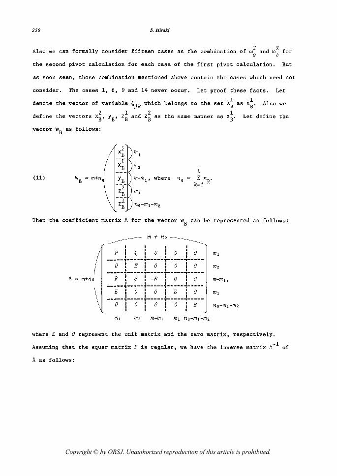
Also we can formally consider fifteen cases as the combination of w; and w~ for

the second pivot calculation for each case of the first pivot calculation. But

as soon seen, those combination mentioned above contain the cases which need not

consider. The cases 1, 6, 9 and 14 never occur. Let proof these facts. Let

denote the vector of variable t,jk which belongs to the set 1 1 XB as XB. Also we

define the 2 2'1 and 2

the same manner as vectors XB

, YB, B ZB as xi. Let define the

vector WB

as follows:

xl. E;

m1

1 XE, m2

l (11) W

B = m+no YE; m-ml

, where no 2: nk. -;2- k=l

E; m1

-zT Eo nO-ml-m 2

Then the coefficient matrix A for the vector WB

can be represented as follows:

A = m+no

._______---- m + no _______________

I

P I Q 0 I 0 0 ml I I I I -----1-----.-----'-----1-----

o : E : 0 : 0 : 0 m2 I I I I

-----~-----~-----~-----,-----R : S : -E : 0 : 0 m-m),

I I I I

-----,-----·-----T-----~-----E : 0 : 0 : E : 0 ml

I I I I

-----'-----T-----~-----~-----o I 0 : 0 : 0 : E nO-ml-m2 I I I I

where E and 0 represent the unit matrix and the zero matrix, respectively.

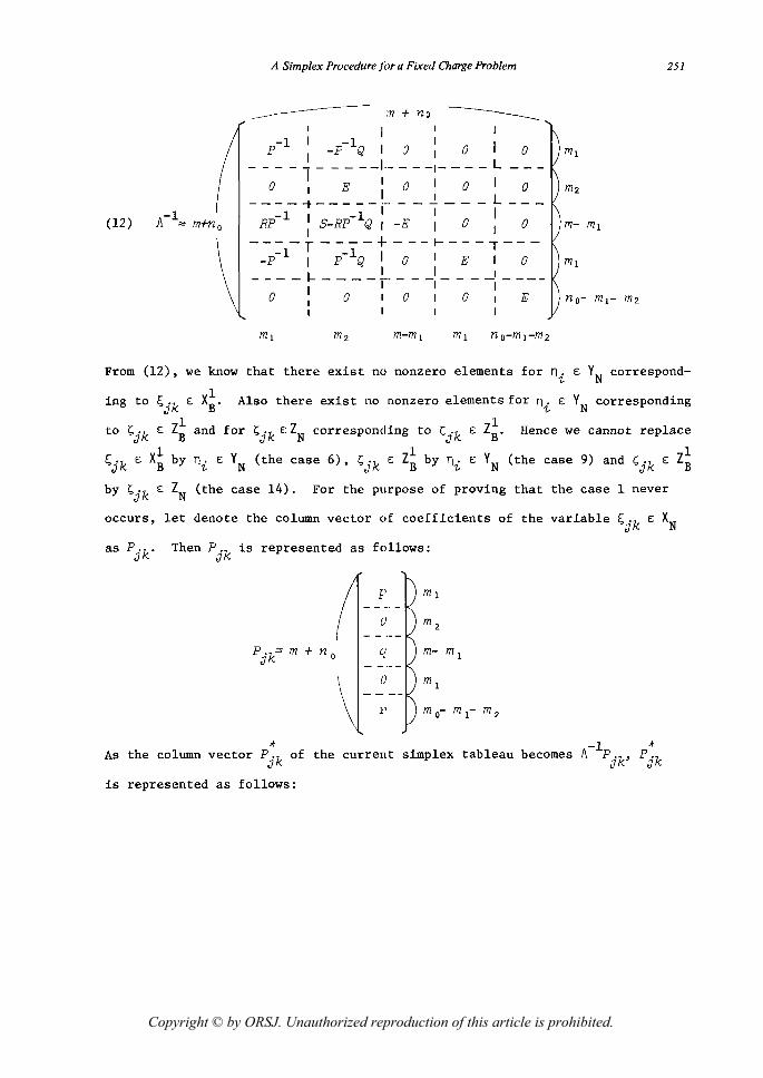
Assuming that the squar matrix P is regular, we have the inverse matrix A- l of

A as follows:


A Simplex Procedure Jc)r a Fixed Charge Problem 251

__________ .71 + no _______

I

(12) -1

l\ == m+no

p-1 1 _p-1Q 1 J : 0 I 1 _______ 1 ____ -1_ - - - L

o I 1 0 1 0 1 1 Ell

- - - - -t - - - - - -- - - - - - L -1 1 -1 1 1 I

RP 1 S-RP Q 1 -E 1 0 1 0

----T----+---r---T---_p- 1 1 p-1Q 1 0 1 E 1 0

- - - - I-- - - - - .!.._ - - -I ____ I ___ _ 1 I I 1 000

o

\ o

o

E

m-ml nO-ml-m2

From (12), we know that there exist no nonzero elements for ni

E YN

correspond-

1 ing to ~jk E XB, Also there exist no nonzero elements for n

i E Y

N corresponding

1 to Sjk E ZB and for

1 ~jk E XB by ni E YN

Sjk E: ZN corresponding to Sjk 1

(the case 6), Sjk E ZB by ni

1 E ZB' Hence we cannot replace

E YN (the case 9) and ~:jk E Z~

by Sjk E ZN (the case 14), For the purpose of proving that the case 1 never

occurs, let denote the column vector of coefficients of the variable ~jk E XN

as Pjk , Then Pjk is represented as follows:

P ml

0 m2

Pjk== m + no q m- ml

0 ml

l' m 0- me m2

* -1 * As the column vector Pjk

of the current simplex tableau becomes A Pjk

, Pjk

is represented as follows:


252 S. Hiraki

(13)

( -1 P P m1

-------

0 mz --------

* -1 RP-1p Pjk= It Pjk m + no - q m- m1 --------

-1 -P P m1

--------

l' no- ml- mz

From (13), we know that there exist no nonzero elements for C,jk € XN

correspond

ing to C,jk € Xi, Hence we cannot replace C,jk € Xi by C,jk € XN' Thus we know

that the cases 1, 6, 9 and 14 never occur.

And yet, for the case 7, 11 and 12, we know that it is enough to investigate

the value ~l' Therefore we may consider the combinations of remaining eight

cases for the twice pivot calculations. But if the basic variable which moves to

the nonbasis in the second iteration does not concern the fixed charge, it is

meaningless for the purpose of decrease in the objective function. After the

consideration of these facts, meaningful twice pivot calculations in our a1gori-

thm become as Table 1.

Table 1. Meaningful pivot calculations

the first pivot calculation the second pivot calculation

2 XN

2 1. Ws € XB' wt € 1. Ws € XB' wt € XN

VB' XN

2 YN 2. Ws € wt € 2. Ws € XB' Wt €

1 XN

1 ZN 3. Ws € ZB' wt € 3. Ws € XB' wt €

2 XN

2 ZN 4. Ws € ZB' wt € 4. Ws € XB' wt .::

5. Ws € Y B' wt € YN 2

€ YN 6. Ws € ZB' wt

7. Ws € VB' wt € ZN 1

€ ZN 8. Ws € ZB' wt


A Simplex Procedure for a Fixed Charge Problem

In Table 1, when we choose the variable wt E XN

to enter the basis for the

first or the second pivot calculation, it is apparent that we should only

consider f,j:l.+1k E XN as the candidate variable of wt

for each k (k=l,----,l),

253

1 2 where we assume that f,j*k E (XB U XB) (k=l,---,l). Also, when we choose the

variable wt

E ZN to enter the basis, \-Ie should only consider l,j*_lk E ZN as the

candidate variable of wt

for each k (7<=1, ---, l), where we assume that s'i *k E . (Z~ U Z~) (k='l,---, l). Moreover, if a basic variable f,j*k* E (X~ U X~) is chosen

to be replaced by f,hk* E XN

(h=j*+l,---,nk

), it is apparent that the objective

function doe.s not decrease. So we may delete such cases in the pivot calcula

tions. Also we may delete to replace a basic variable Sj*k* E (Z~ U Z~) by

l,hk* E ZN (h=l,---,j*-l).

4. Algorithm

In this section, we will propose the computational procedure to solve the

fixed charge problem def ined as Prob lem B. The fundamental idea is bas.~d on

the simplex method of linear programming. Though this algorithm seems to re-

semble the heuristic method proposed by Steinberg [6] and Walker [7], it is

slightly different from [6] and [7] ill respect of selecting the pivot element by

utilizing properties of the problem. We prepare two kinds of simplex tableau

for the algorithm, that is, S-&mplex T,"bleau 1 (ST1) and Simplex Tableau 2 (ST2).

We use ST1 for the pivot calculations when variables to enter the basis and

move to the nonbasis are determined. On the other hand we use ST2 only for the

purpose of calculation of Ni2

• The ba.sic computational procedure is constructed

from Step 1 to Step 14. We use ST1 from Step 1 to Step 6 and Step 13 to Step 14,

ST2 from Step 7 to Step 12 in the a1gcrithm.

Step 1. Solve Problem A by using ordinary simplex method.


254

Step 2.

Step 3.

(14)

Step 4.

(15)

S. Hiraki

Set j +- 1, F +- 00, CLnd II +- 1.

If W. E: WB

, go to Step 13. Otherwise determine the basic variable J

w. E: WB

according to (14) , 1-1

e. min {e. 1* 1* for

1* > O} S. / a . . , a .. 1-1

l~i:5fn+no 1- 1- 1-J

where 1*

is the (i., j) element of a .. 1-J

Calculate the value,

1 1 Ml = (y. - n.) e. J J 1-1

fj,H 1 by (15) ,

1 1 +(0.-0.). J 1-1

a) if fj,Hl < 0, then go to Step 6,

b) if fj,H 1 ~ 0, then go to Step 7.

1-J

current ST1.

that is,

Step 6. Compare fj,H 1 with F:

b) if F ,:s fj,H 1 , go to Step 13 at once.

Ust ST2 from Step 7 to Step 12.

Step 7. Set each element of ST2 as the same value as ST1.

Replace w. E: WB by W. E: WN

and set k +- 1. 1-1 J

Step 8. If Wk

E: WB

, go to Step 12. Otherwise determine the basic

variable w. E: WB 1-2 according to (16).

min {e. 2* 2* for

2* > O}, (16) e. S. / aik~ aik 1-2

1~i~m+no 1- 1-

2* where a

ik is the (i,k) element of current ST2.

Step 9. Calculate the, value of M2 by (17):

(17)

Step 10. For fj,H2:

a) if M2 < 0, then go to Step 11,


A Simplex Procedure /or a Fixed Charge Problem 255

b) if M2 2:, 0, then go to Step 12.

Step n. Compare 6.H2 with F:

~ + 3 and go to Step 12,

b) if F ~ M 2 , go to Step 12 at once.

Step 12. Set k + k+1:

a) if k ~ m+2no, then go to Step 8,

b) if k > m+2n o, then go to Step 13.

Step 13. SE~t j + j+1:

a) ifj ~ m+2n o, then go to Step 3,

b) ifj > m+2n o, then go to Step 14.

Step 14. For ~:

a) if ~ 1, the algorithm is terminated,

b) if ~

return to Step 2,

1* c) if ~ = J, replace w

S1 by w

t1 by pivoting on term 0Sltl for the

fi.rst pivot calculation and then replace WS2

by wt2

by pivoting on

2* te,rm 0 t for the second pivot calculation. Return to Step a.

S2 2

If various methods are contrived under the consideration of the properties

mentioned in chapter 3, we can improve the efficiency of the algorithm" Let

jr/X) (k=l,---, l) be the maximum number of subscript of t,jk such that l;jk E (X!

U X;) for each k and define J*(X) = {jl(X),---,jZ(X)}. Also let jk(Z) (k=l,---,

l) be the minimum number of subscript of Sjk such that Sjk E (Zi U Z;) for each

k and define J *(Z) = {jl(Z),---,jZ(Z)}. Store the current J*(X) and ~I*(Z)

after solving Problem A and at any step of the pivot calculation, that is, at

Step 1 and Step 14. Then we can contrive the algorithm as follows:

a) It is enough to investigate only t,j*+lk E XN for each k and only Sj*_lk


256 S. Hiraki

E: ZN for each k at Step 3 and Step B.

b) When determining the basic variable which moves to the nonbasis by using

1 eq. (14) in Step 3, we only consider such subscript that i. E: J*(X} for w1: E: (X

B 2 1 2 U XB) and i E: J*(Z} for w

i E (ZB U ZB)' Also when determining the basic vari-

able which moves to the nonbasis by using eq. (16) in Step B, it is enough to

investigate such variable that wi E: (X~ U X~) and i E: J*(X}.

5. Numerical Experiments

5.1 Numerical example

To illustrate the a1goxithm mentioned in chapter 4, we show a simple

numerical example. Let consider the problem of minimizing

F = [-L :3 5 ~] c-5 5 5 5 s11

t;,2.1

t;,3_1

t;,4.1

+ [10 15 20 25] [t;,11]

subject to

[t;,21]

[t;,31]

[t;,41]

t;,11

t;,21

t;,31

t;,41

o ~ t;,jk ~ 1 (j=l,---,nk; {if k=1,---,3} if

t;,jk>O, then t;,ik=l for

t;,jk=O, then t;,ik=O for

C k ={ 1 if t;,jk > 0

J 0 if t;,jk = 0

3 3

i=l,---,j-l

1..=J+l,---,nk

(j=l,---,nk

;

The optimal state of Problem A is shown in Table 2 and Figure 3.

(k=l,---, 3),

k=l,---,:3).


Table 2. Optimal tableau of Problem A~

°jk 10 15 20 25 5 10 15 10 10 10

1 3 5 7 1 3 1 5 1 3 5 Yjk 5 5 5 5 6 6 6 3 3 3

dB 1 cB wB b 1['11 [,21 [,31 1 [,41 [,12 [,22 [,32 [,13 [,23 [,33 n1 n 2 n3 [,11 [,21 1[,31

5 1

[,12 1 1 6

10 3 [,22

2 1 1 -11 -2 7

6 15 30 3 30

10 1

[,13 1 1 3

10 1 [,11

I

5 1 1 1 3

[,21 li I I i 151 5 1 1

20! -%,[,31 !1~ I I I

11 1! i

! I 1 1 .:21 --.i1-13 I -1 -1 I i ! 30, 1~, 30: S! "="3 i 1.-, .~n~ 7!;i :~(),

[,41 1 1 I

10 3

[,23 ! 2 I I ! 1! 11

1 -1! 1 ! -I

1 -3 3 6 3 6

[,22 13 I -1

11 1 -7 15 30 15 30

--

[,32 1 1

[,31 8

-11 , 1 -4 13

1 1 1 15 30 15 3D

[,23 1

-1 -1 1 -1

3 6 3 6

[,33 1 1

2.5 2 1 2 1 1 3 4 2

Yjk- Trjk 5 3 3 20 10 20 5 5

6Jh 182

.5

1 I I 13~~1 12~il 4113] 113471 32

116

1 "9 110 10 -35 75 75

~ We assume that each empty element in the tableau takes the value zero.

[,41 [,12 [,22 [,32

1

-1

I

1 1 1 I !

1 I I ! ! ! !

1 1 -~f--

1

1

1 3"

I ~~I I I

[,13 [,23

1

! 1

-1

1 1

2 3"

~I I

[,33

1

::...

~ W ~ ~ ~ '0' ... '" ~ '" Q.

9 '" ~ '" ~ "'" '" ;;

'" v.

" Copyright © by ORSJ. Unauthorized reproduction of this article is prohibited.

'EY'l , J J

I 71-_

Y41~ I 51

3 Y ~---1IY21~12. 5 t

Y 11=:st-- 51 I I

[,41 H, t [,11 I

j J1 ? t I I ,

641=25:

t , 451 t t l' t

611=1°1

, 6 -20' 31- I , I ' ~ 1 • 1

621=151 1 ,

-+

[,11 [,21

b~ I [,31 [,41

'EY'2 , J J

1 Y 12=---0&

E[, , I j J1 - I I

E6, , J <

J

I I I

? + 1

632=151 I I

1

.....

'EY'7 j JUI I I

H, j J ~

20

1----

.(~5 I I 33 3, I 3 L..___ 1

Y 23-3 1 I 1 I

[,33

, I

9 ~ 633= 10 1

, 1

I 1 1 Y 1 1

623=lq 1 I 1 1

I 1 I I 1

°12=5 °13=10

; 1 I 1 I 3 I 1

I

E['-i1 [,12 j ,,- [,22 [,32 E[,-i2 j "

Fig, 3 Optimal state of PY'obZem A

I '11' 1

[,13 [,23 [,33

u; '3 , J J

E["3 ,J J

"" v, 00

'" ~ ., i!!:



The value of the objective function it; F = 82.5. According to the algorithm,

we have the values of 6.H1 and M2 as Table 3.

Table 3. Values of 6.H1 and 6.H2 for Table 2

piv the first the second values of 6.H1 and ~. ·ot calculation pivot calculation

1 1 2 2 M1 M2 W w

t W w

t s 8 ----

~23 ~32 13/110 -95/22

/;22 III ~31 112 13/110 -97/10 ------

~23 113 13/110 -97/10 ---

~31 ~33 1/10 -229/24

-------

/;23 112 ~31 III 1/10 -197/10* ------ --

~22 113 1/10 -97/10

~22 113 /' / -1045/105 ~ * Minimum value of 6.H 1 and M 2 •

From Table 3, we know that

pivot calculation and then

we should replace /;23 E

2 ~31 E XB by III E YN for

2 ZB by 112 E YN for the first

the second pivot calculation.

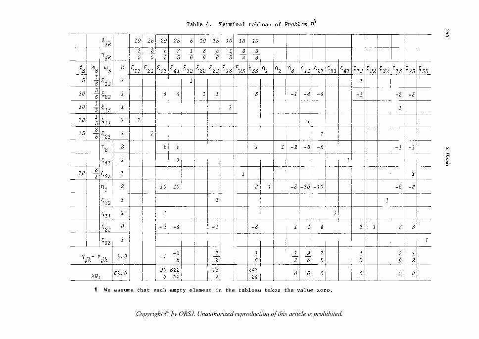
After these pivot calculations we have the state shown in Table 4 and Figure 4.

The value of the objective function is F = 62.8. For Table 4, we have the

values of 6.81 and M2 as Table 5. As there exists no 6.H1 or 6.H2 which takes

the negative value, we know that Table 4 shows the terminal state of Pr'oblem B.


Table 4. Terminal tableau of Problem B~

°jk 10 15 20 25 5 10 15 10 10 10

1 3 5 7 1 3 5 1 3 5 Yjk - -

5 5 5 5 6 6 6 3 3 3

dB cB WB b [,11 [,21 [,31 [,41 [,12 [,22 [,32 [,13 [,23 [,33 111 112 113 [,11 [,21 [,31 [,41 [,12 [,22 [,32 [,13 [,23 [,33

5 1

[,12 1 1 1 6

10 I 3

[,22 1 i 1 4 4 1 1 3 -1 -4 -4 -1 -3 -3 6

10 1

[,13 1 I I I

11 1 3 I i 10, 1

1 I I ! I I --,:[",1 1 I I I I I I 1 1 1 1 I iJ I .11. I I I I I I I I I I I I I I I I I I I I

15

1 t:' j : I 1'1 ,f: I 11 11 11 IIlll4 1,1 I I ]-,I -1: 1 31 ~411 1 1 1 1 ~t' -I 1 1 I 1 -+---i-tn +---i-~ j r- +.-+t---_·t- -- ~--t-+-

10 3[,23 1 1 I I I I I I I I 11 1 I 1 1 I I I 11

I 1111 I 2 I 1 110

110

I I I I I I 81 1 I 1 ~3 -10 -10 I I I -81 -8

::: I : i : : 1 I ; ,; I ' 1 - I i~jnj-+------t- ! ! i i -t!! 1 -+--+-+---+--+--

I 1[,221 0 I i ! -4 -41 L 1 -1 1 -31 1 I 1 4 41 1 1 11 11 1 ~ : I 1 -

[,33 1 i ; i

I -3 I 1 11 j I I Yjk- Tfjk 2.~ -1 5 I : 31 6 i I I

1 1 ,t- il' I 1 ! I . ! , , 1 ! 1 Inn '11 991622, i 116 I 2411 '1i "I '11 i i /11 I /1 /1. 6H 1 1 D 6. 0 j L j 51251 1 1 3-1 j 1241 1 1 U I U I vII 1 vII 1 V 1 V 1

~ We assume that each empty element in the tableau takes the value zero.

'" 0-

""

~

El; i:! i5:


Yll

[0. j J1

I I

~ t 1 1 1

o -25 1 4F 1

1

I !

~ + 1

o -20 1 31- I

1 I

25.--,

I 0

21=151

I I

"1 011=1 q I

I

[.11 [.21 .. [.31 [.41

[Y'2 . J J

[0. j J2

15

• I'

I

? 1

032

=15 1 I I

022=ln

l

+ 1 t 012

=5 I ,

1:[.'1 . J J

~12 ~22" [.32

[0 . j J3

I I

o =10? t 33 1

I 20 J-----O---........

023=10: I

t t 013=10

[~'2 . J J

, . ~13 ~23" ~33

Fig. 4 Terminal state of ProbZem B

[~ '3 • J J

[~'3 . J J

~

{ ~

~

i ';:;>. ~

'" ~ 2-9 !:l ~

~ "'" [

'" '" .....


262 S. Hiraki

Table 5. Values of t:.HI and t:.H2 for Table 4

the first the second values of t:.HI and t:.Hz pivot calculation pivot calculation

1 1 2 2 t:.HI t:.Hz W w

t W w

t s s

1;33 1;31 8/81 1207/60 n1 1;33 1---

1;22 n3 8/81 5/4

5.2 Results of numerical experiments

In order to test the effectiveness of our algorithm mentioned in this paper,

we prepare some numerical examples with the following properties:

(1) l = 5, m = 5, nk= 5 (k=l,---,lJ, hence no= 25, m + no = 30 (the number of

inequalities) and m + 2no = 55 (the number of variables including slack),

(2) (i=l,---,m; j=2,---,nk; k=l,---,lJ

and 0 ~ Ui1k ~ 9 (i=l,---,m; k=l,---,lJ,

(3) Sik are given about 0.6 times as many as L uijk for all i and k (i=l,---,m; j

k=l,---,lJ, and

Table 6 shows the input data we used. For each coefficients matrix and

vector (Ak,bJ of Table 6 (a), we examined all the cases of the cost and the fixed

charge vector (ck,dkJ of Table 6 (b), that is, we solved 5 x 4 20 cases.

Table 7 shows the results of numerical experiments. In Table 7, case 1-2, for

example, implies that data no. 1 of Table 6 (a) and data no. 2 of Table 6 (b)

are combined.



Table 6. Input data for the numerical experiments

(a) Coefficients matrix and vector (A1(,bJ

data no. A1 A2 A3 A4 A5 b

2 2 222 3 3 3 3 3 2 2 2 2 2 2 2 2 2 2 0 000 0 30 22222 6 6 6 6 6 9 9 9 9 9 0 o 0 o 0 6 666 ti 70

1 5 5 5 5 5 3 3 3 3 3 8 8 8 8 8 7 7 7 7 7 0 000 0 70 5 5 555 7 7 7 7 7 0 o 0 0 0 0 o 0 o 0 5 5 5 5 ,-

,) 50 66666 4 4 4 4 4 e 6 6 6 6 4 4 4 4 4 3 3 3 3 :3 60

6 6 6 6 6 7 7 7 7 7 2 2 2 2 2 5 5 5 5 5 8 888 (I 80 4 4 4 4 4 1 1 1 1 1 1 1 1 1 1 7 7 7 7 7 9 9 9 9 9 60

2 9 999 9 9 9 9 9 9 0 o 0 o 0 3 3 3 3 3 o 0 0 0 0 60 3 333 3 3 3 3 3 3 0 o 0 o 0 3 3 333 555 5 r

,) 40 3 3 3 3 3 4 4 4 4 4 3 3 3 3 3 6 6 666 8 8 8 8 B 70

2 2 222 8 8 8 8 8 2 2 2 2 2 7 7 7 7 7 3 3 3 3 ij 70 9 9 9 9 9 o 0 000 4 4 4 4 4 1 1 1 1 1 o 0 o 0 0 40 4 4 4 4 4 1 1 111 v 6 6 6 6 0 o 0 o 0 2 2 2 2 .)

(, 40 8 8 8 8 8 o 0 000 9 9 9 9 9 7 7 7 7 7 3 3 3 3 ij 80 9 9 999 9 9 999 4 4 4 4 4 8 8 8 8 8 o 0 o 0 0 90

7 7 7 7 7 9 9 9 9 9 2 2 2 2 2 3 3 3 3 3 2 2 2 2 .) (, 70

2 2 2 2 2 4 4 4 4 4 8 8 8 8 8 7 7 7 7 7 7 7 7 7 " 80 I

4 3 333 3 6 6 6 6 6 7 7 7 7 7 7 7 7 7 7 6 6 6 6 ti 80 6 6 666 1 1 1 1 1 7 7 7 7 7 1 1 1 1 1 9 9 9 9 g 70 55555 5 5 5 5 5 2 2 2 2 2 7 7 7 7 7 7 7 7 7 " 80 (

0 1 2 3 4 8 8 8 8 8 0 o 0 0 0 6 6 6 6 6 8 888 B 70 1 2 3 4 5 4 4 4 4 4 222 2 2 3 333 3 6 6 6 6 ti 50

5 5 6 7 8 9 9 9 9 9 9 888 8 8 9 9 9 9 9 6 6 6 6 ti 120 3 456 7 5 5 555 o 0 000 222 2 2 5 5 5 5 r

,) 50 0 o 1 2 3 o 0 0 0 0 o 0 000 1 1 1 1 1 1 1 1 1 } 10

(b) Cost and fixed charge vector (ck' dk )

date no. cl c2 c3 c4 c5 d1 d2 d3 d4 d5

25 20 60 80 60 100 150 200 250 ;)00 30 25 65 85 65 110 160 210 260 ;UO

1 35 30 70 90 70 120 170 220 270 ;l20 40 35 75 95 75 130 180 230 280 ;l30 45 40 80 100 80 140 190 240 290 ;l40

60 80 60 20 25 100 150 200 250 ;WO 65 85 65 25 30 110 160 210 260 ;l10

2 70 90 70 30 35 120 170 220 270 ;l20 75 95 75 35 40 130 180 230 280 ;l30 80 100 80 40 45 140 190 240 290 ;]40

25 20 60 80 60 300 250 200 150 :100 30 25 65 85 65 310 260 210 160 no

3 35 30 70 90 7e 320 270 220 170 :720 40 35 75 95 7.5 330 280 230 180 :130 45 40 80 100 80 340 290 240 190 :140

60 80 60 20 25 300 250 200 150 :100 65 85 65 25 30 310 260 210 160 no

4 70 90 70 30 3.5 320 270 220 170 .120 75 95 75 35 40 330 280 230 180 .130 80 100 80 40 45 340 290 240 190 :140


264 S. Hiraki

* Table 7. Results of numerical experiments

values of the number of pivot decrease in time §

data objective function calculations after the objective Problem A'IT Problem B solving Problem At function (sec. )

case 1-1 2924.44 2878.33 1 ( 0, 1 ) 46.11 20.7

case 1-2 4324.44 4096.95 3 ( 0, 3 ) 273.49 34.9

case 1-3 4413.96 4097.38 1 ( 0, 1 ) 316.58 21.0

case 1-4 4113.96 3997.38 1 ( 0, 1 ) 116.58 21.1

case 2-1 3633.33 3451>.67 1 ( 1, 0 ) 176.66 20.3

case 2-2 3480.00 3480.00 0 ( 0, 0 ) 0.00 16.2

case 2-3 3633.33 3318.3.3 1 ( 1, 0 ) 315.00 21.2

case 2-4 3280.00 318/).87 3 ( 0, 3 ) 93.13 37.3

case 3-1 3538.67 3271).00 1 ( 0, 1 ) 263.67 23.5

case 3-2 4891.97 374;;' 00 7 ( 0, 7 ) 1148.97 57.8

case 3-3 4738.67 4:11;).00 5 ( 0, 5 ) 523.67 47.0

case 3-4 4391.97 4081i.00 4 ( 1, 3 ) 306.97 43.5

case 4-1 4181.19 3930.00 2 ( 0, 2 ) 251.19 27.7

case 4-2 4620.96 408;~.94 4 ( 2, 2 ) 537.02 40.5

case 4-3 4181.19 373i1.04 4 ( 1, 3 ) 442.15 42.1

case 4-4 4220.96 370~i.00 2 ( 0, 2 ) 515.96 27.1

case 5-1 3671.25 342:). 50 1 ( 0, 1 ) 248.75 6.5

case 5-2 4708.75 370;;' 00 9 ( 1, 8 ) 1005.75 16.7

case 5-3 4571.25 3790.00 6 ( 0, 6 ) 781.25 13.5

case 5-4 3708.75 3636.00 1 ( 0, 1 ) 73.75 6.6

* The computer used is the HITAC 8700 with 05/7 at the Computer Center of Hiroshima University except for the case 5.

'IT The value of the objective function eq. (1) for the solution of Problem A.

t Total number of pivot calculations (the number of once pivot calculation (the case ~ = 2). the number of twice pivot calculations (the case ~ = 3».

§ The computer used for the case 5 is the HITAC M-180 with vaS3.



6. Conclutions

We propose an approximate solution method for the problem defined in the

introduction. As the algorithm mentioned in chapter 4 is based on the simplex

procedure, we can easily treat our problem. If we are in the situation in

which the more precise solution must be determined, we will prepare thr(~e kinds

of simplex tableau for the algorithm and define the decrease in the obj(~ctive

function after three times of the pivot calculations. But it is apparent that

the more the, pivot calculations increase, the more the computational time and

the computer memory required increase.

Acknowledgements

The author wishes to thank ProfeE.sor Kenichi Aoki of Hiroshima University

for his helpful comments, and to the referees for their kind and useful comments.

This work was supported by the Zaidan Hojin Keiei Kagaku Shinko Zaidan.

References

[1] Aoki, K. and Hiraki, S.: A Study on Production Schedule for the Conveyer

Line System. Transactions of the Japan Society of Mechanical Engineers.

Vol. '+0, No. 340(1974), 3542-15~)3 (in Japanese).

[2] Cooper L. and Drebes, C.: An Approximate Solution Method for the Fixed

Charge Problem. Naval Research Ttogistic Quarterly. Vol. 14, No. 1(1967),

101-113.

[3] Had1ey, G.: Nonlinear and Dynamie Programming. Addison-Wes1ey, 1964.

[4] James, A. P. and Soland, R. M.: A Branch-and-Bound Algorithm for Mu1ti

level Fixed Charge Problems. MalU1gement Science. Vol. 16, No. 1(1969),

67-76.


266 S. Hiraki

[5] Mine, H.: Operations ReHearch (Vol. 1). Asakura Shoten, 1966, 134-142

(in Japanese).

[6] Steinberg, D.!.: The Fixed Charge Problem. Naval Research Logistic

Quarterly, Vol. 17, No. 2(1970), 217-235.

[7] Walker, W. E.: A Heuristic Adj acent Extreme Point Algorithm for the Fixed

Charge Problem. Management Science, Vol. 22, No. 5(1976), 587-596.

Shusaku HIRAKI: Department of Systems

and Industrial Engineering, Faculty

of Engineering, Hiroshima University,

Senda-machi, Naka-ku, Hiroshima, 730,

Japan.


Date post:	08-Apr-2022
Category:	Documents
Upload:	others
View:	3 times
Download:	0 times

which contains semi-variable costs represented as a ...

Documents