Who Creates and Destroys Jobs over the Business...

Who Creates and Destroys Jobs over the Business Cycle?

Andrea Colciago, Volker Lindenthal, Antonella Trigari

July 29, 2016

AbstractWe study the cyclical properties of job flows of young versus mature and small versus large firms,as well as their contribution to aggregate employment fluctuations, with a particular emphasis onthe Great Recession. For the period of the Great Recession we document that young firms arehit harder than mature firms. In contrast to previous studies we find that size differences amongfirms do not play a major role in explaining heterogeneity in job flows in the Great Recession.The general business cycle behavior for the period 1982-2013 are confirming the findings for theGreat Recession.The overall contribution of young firms to employment fluctuations, however, is limited. The largeremployment weight of mature firms – mature firms employ around 80 percent of the labor force –more than compensates for their smaller cyclicality.

1

1 Introduction

Among economists and policymakers the belief of small businesses being the engine of job creationand innovation is widely spread.1 In 1953 the Small Business Administration (SBA) was foundedas an independent agency of the federal government with the goal to “aid, counsel, assist andprotect the interests of small business concerns”. Discussions about heterogeneous effects on firmsare often dominated by the distinction between small and large businesses, neglecting the role offirm age.We do not challenge the conventional view about small businesses per se,2 but rather contributeto the discussion on the cyclical sensitivity of small and large firms. In particular, we contributeto this discussion by emphasizing the awareness of firm age as important determinant for cyclicaljob flows of firms. We ask the general question of who creates and destroys jobs over the businesscycle? And in particular who is hit harder during the Great Recession?This study contributes to two separate, but related questions on the cyclicality of job flows and thecontribution of different groups of firms to employment fluctuations. First, we investigate whichgroup of firms in terms of age and size is more sensitive to the cycle. There is a growing scientificinterest in determining the cyclicality of large versus small and young versus mature firms. WhileMoscarini and Postel-Vinay (2012) show that large firms are more sensitive compared to smallfirms in periods of high and low unemployment, Fort, Haltiwanger, Jarmin, and Miranda (2013)highlight the importance of firm age and argue that firm age is of particular importance when itcomes to small firms. Our findings are closer to the latter ones. We find that young firms aremore sensitive to the cycle compared to mature firms. Second, we research the contribution toaggregate fluctuations by means of a variance decomposition. Even though young firms are moresensitive to the cycle, their contribution to employment fluctuations is moderate. The reason isthat most workers are employed in mature firms. We show that employment shares are crucial inunderstanding the contribution to employment fluctuations.By better understanding the cyclical behavior of firms in terms of age and size, policymakersmight revise their beliefs and policies. Most policies to support troubled businesses are relatedto the size of firms, while the economic arguments are rather related to the age of the firmsand their growth potential. Furthermore, knowing the actual contributions of different firms toaggregate employment fluctuations helps to evaluate costs and benefits of certain measures tostabilize employment. Very volatile firms might be sensitive to the cycle, but contribute only littleto the aggregate fluctuations due to a little weight in the economy. Thus, depending on the goalsand costs it might be better to support less sensitive firms as they contribute more to the cyclicalfluctuations.Our main findings are that for the period of the Great Recession there is no heterogeneous behaviorof small and large firms. The main source of heterogeneity is the firm age instead. We findthat firms younger than 5 years are hit harder than mature firms. However, when measuringthe actual contribution to overall employment volatility the findings revert. Because of theirsmall employment share young firms contribute relatively little to overall employment fluctuations.

1An important and interesting analysis of small businesses is provided by Hurst and Pugsley (2011). They arguethat the conventional view on small businesses in economic models has important caveats. In particular, manysmall business owners are neither interested in growing large nor innovating, but rather provide an existing serviceto an existing market.

2In particular, we cannot add to the discussion on the general behavior of small businesses as we focus on thebusiness cycle only.

2

Instead, mature firms contribute the lion’s share.Results for the period from 1982 to 2013 confirm our findings for the Great Recession and showthat young firms are more sensitive than mature firms. Moreover, we document that the jobcreation and destruction due to actual entry and exit of establishments is relatively less importantcompared to the expansion and contraction of existing establishments.The paper is structured as follows. The following section discusses the data as well as relevantmeasures and the empirical strategy for the analysis. The third section discusses results for thecyclical behavior of different groups of firms and their contribution to aggregate fluctuations with aparticular emphasis on the Great Recession. The fourth section briefly discusses existing policies,while the last section concludes.

2 Data, Measures, and Empirical Strategy

The main dataset that is used in this study is the Business Dynamics Statistics (BDS) database.The BDS is often used to analyze cyclical labor flows despite being on an annual frequency. Becauseit covers a long period, starting from the late 1970’s, it allows to analyze several business cycles.3

We classify firms according to size and age. We define size as follows: Small firms are those withemployees of less than 50, medium size firms are those with employees between 50 and 1000, andlarge firms those with more than 1000 employees. As shown in table 1, our classification is in linewith the size classification applied by Moscarini and Postel-Vinay (2012). Fort et al. (2013), incontrast, define the small firms more restrictive by applying lower size cut-offs.4 The age definitionis as follows: Young firms are those of age 0 to 5 years, mature firms are older than 6 years.

Table 1: Overview of AGE and SIZE Classification in the Literature

Study Age Size Treatment ofCyclical Job Flows

Moscarini and Postel-Vinay (2012) No Age Small: 0-49 HP-FilterMedium: 50-999Large: 1000+

Fort et al. (2013) Young: 0-4 Small: 0-19 Pure RatesMature: 5+ Medium: 20-499

Large: 500+

Pugsley and Sahin (2015) Young: 0-10 Small: 1-19 Linear TrendMature: 11+ Medium: 20-499

Large: 500+

The table gives a brief overview of age and size definitions of other studies in the literature. Furthermore, itreports the treatment that was applied when analyzing cyclical job flows.

Throughout the analysis we use three groups – GROUPS = {SIZE,AGE,AGE/SIZE} –

3Some studies relate also to the Business Employment Dynamics (BED) database provided by the US Bureauof Labor Statistics. It comes on a quarterly frequency, but is not suitable for our purposes as it does not report theage of firms and covers a shorter period, starting from 1992.

4Appendix 15 reports results with these alternative size cut-offs of Fort et al. (2013).

3

to investigate the role of size and age. The individual groups are composed of the following set offirms:

• SIZE = {SMALL,MEDIUM,LARGE}

• AGE = {Y OUNG,MATURE}

• AGE/SIZE = AGE × SIZE5

2.1 Business Dynamics Statistics (BDS)

The administrative BDS dataset is provided by the US Census and covers approximately 98 percentof the nonfarm private-sector employment in the United States.6 It is based on the LongitudinalBusiness Database (LBD) and contains information on establishment-level job flows and employ-ment stocks for continuing as well as entering and exiting establishments at an annual frequency forthe period 1976 to 2013.7 The data can be broken down by location and industry of the establish-ment, as well as by age and size of the parent firm. A firm is thereby simply defined as a collectionof all its establishments. The age of a firm is defined by the age of its oldest establishment. Firmsize is measured as the sum of all employees in its establishments.Two notions of firm size are reported in the BDS: On the one hand, size is measured by initial

firm size, which captures the size of firms at the beginning of a period, i.e. t− 1, before job flowstake place. It is our preferred measure as it is not subject to the reclassification bias.8 On theother hand, size is reported as the average firm size between year t− 1 and year t.9

Employment for each establishment is measured by the number of employees reported at March12 for each year. Therefore, the job flows for a given year t are measured between the employmentstock of year t− 1 year t.Establishment age is computed by taking the difference between the current year of operation andthe birth year and readily available in the BDS. Given that the LBD series starts in March 1976observed age is by construction left censored. Given our age threshold we can only start in 1982,which allows us to distinguish between firms of age 5 and those that are 6 years and older. Thus,our sample period is restricted to the years 1982 to 2013.In principle, the BDS allows to use all information broken down by initial firm size as well as age.The only exception are the new born firms, which are reported according to their end of periodsize. We follow Moscarini and Postel-Vinay (2012) and re-classify new firms according to their

5The group of Y OUNG/LARGE is dropped from the analysis as will be discussed in section 2.2.6An extensive description is available on the website of the Census at

http://www.census.gov/ces/dataproducts/bds.7The BDS tabulations can change over time, because new longitudinal information on the underlying LBD is

becoming available. The 2013 version of the dataset is improving in the accuracy, because it ends with a EconomicCensus year in which the quality of the underlying microdata is higher.

8The reclassification bias is also known as the size distribution fallacy and stems from the fact that the job flowsare not correctly attributed to the right firms. As soon as firms are changing between size groups outcomes differdepending on whether flows are attributed to the size groups at the beginning of the period or to the groups definedby the current size. Davis, Haltiwanger, and Schuh (1996, p. 62ff.) provide a further discussion including numericalexamples of this issue.

9To investigate the potential regression bias (Davis et al., 1996, p. 66ff.), one could use both size measuresfor comparison. The regression bias emerges when a given firm is constantly oscillating between two size groupsand therefore systematically biasing the smaller group upward and the larger group downward. Moscarini andPostel-Vinay (2012) have shown that this bias is not strongly pronounced for the BDS at the cyclical frequency.

4

beginning of period size, i.e. 0 employees. This consistency in defining all firms with their initialperiod size comes with the drawback that by definition all new firms are considered small.Firms can change their employment stock either on the extensive margin by opening and closingestablishments or on the intensive margin by expanding and contracting the labor force in alreadyexisting establishments. Gross job gains include the sum of all jobs added between year t − 1and year t at either opening or expanding establishments. Gross job losses include the sum ofall jobs lost during a given year in either closing or contracting establishments. The net changein employment or net job creation is the difference between gross job gains and gross job losses.Thus, if a firm expands one establishment and contracts another one, it will contribute to both,gross job gains and gross job losses, while the net job creation will represent the actual number ofjobs created or destroyed by the firm.10

The BDS exploits information on ownership of multiple establishments owned by the same firm,thus allowing for two notions of entry and exit. On the one hand, one can think of establishmententry and exit, and on the other hand of firm entry and exit. Entering and exiting firms necessarilyoperate on the extensive margin by opening and closing establishments and the jobs they createand destroy are therefore by definition a subset of all jobs created and destroyed by establishmententry and exit.

2.2 Job Flow Measures

There is no dominant measure for cyclical job flows in the literature. Both measures, job flows aslevels and as rates are commonly used. For our purposes, however, and in particular the cyclicalanalysis we are interested in the behavior of employment growth rates of different firms, withouttaking into account their overall employment share in the economy. Thus, for us, the appropriatemeasure is given by the job flow rates as defined below. This measure also allows for comparisonswith recent studies of Moscarini and Postel-Vinay (2012) and Fort et al. (2013).The net job creation rate (NJCR) for s ∈ SIZE – and similar for AGE and AGE/SIZE –is defined as the difference between the job creation rate (JCRs

t ) and the job destruction rate(JDRs

t ), i.e. simply the difference between all establishments with net job gains and those withnet job losses in a given group of firms s:

NJCRst =

∑e∈S+

(Es

e,t − Ese,t−1

)

12

(Es

t + Est−1

)︸︷︷︸

JCRst

−

∑e∈S−

(Es

e,t−1 − Ese,t

)

12

(Es

t + Est−1

)︸︷︷︸

JDRst

, (1)

where Est represents the employment at time t within an establishment that belongs to group s.11

Depending on whether an establishment is increasing or decreasing its workforce it is counted asjob creator (belonging to set S+) or job destroyer (belonging to set S−).Thus, for each of the six AGE/SIZE categories of firms – and of course for any of the moreaggregated SIZE or AGE categories – we generate series of job flow rates. The disaggregatedAGE/SIZE series are quite stable over time and vary mainly over the cycle as shown in figure

10This example underlines that there is no netting out of job flows within a firm. Since we use establishment-leveldata a firm can contribute to both, job creation and job destruction at the same time.

11By dividing through the average employment in group s, this measure provides a symmetric growth rate foreach period t. In principle, it is well-defined for entrants and exiters as well, because the denominator will be alwayspositive.

5

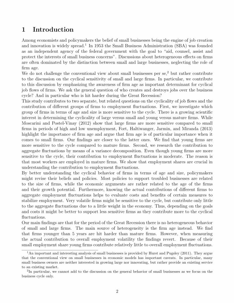
1. The only exception is the group of Y OUNG/LARGE firms, which we drop from the sample.Their rates are very jumpy, because there are not many firms entering the market with more than1000 workers. This problem is further aggravated because the BDS does not disclose informationin many years, because the data would rely on too few firms. Therefore, we decided to dropall job flow rates and employment of the Y OUNG/LARGE category from our analysis. As aconsequence, we re-compute all aggregates, neglecting the existence of Y OUNG/LARGE firms inthe economy.12

Figure 1: Job Flows by AGE/SIZE over Time

The graph plots the BDS job flow rates by AGE/SIZE. NBER recessions are plotted in shaded gray areas. Thegroup of Y OUNG/LARGE firms is dropped from the analysis.

Figure 1 shows that the job flow rates for MATURE firms are within a small bandwidth.13 Onaverage they are negative, meaning that employment is decreasing once firms are growing older.This finding is in line with the findings of Pugsley and Sahin (2015) who show an increase in the em-ployment share of MATURE firms. It indicates that firms grow when they are Y OUNG/SMALLand in particular when they enter the market and destroy jobs on average afterwards. When weinvestigate this issue further by dropping the job flows due to entering firms, we observe that all

12This does not bias our results much as they account for only about 1 percent of overall job flows and employment.13This finding is not dependent on the size cut-offs. Figure 29 in appendix 15 reveals the same patterns for the

size cut-offs of Fort et al. (2013).

6

net job creation rates are on average negative as shown in 20 in appendix 8. This finding highlightsthe importance of the entry margin for overall job creation.Nevertheless, the average job flows of different groups of firms are not at the focus of this study.We are only interested in their cyclical properties. Figure 1 shows that most series are relativestable, but slight trends are visible as well. Therefore, we generally de-trend the data series –unless specified differently. Our preferred method is to linearly de-trend the series.14 For any jobflow rate Xt, denote Xt the trend, we define the cyclical component as deviation from the trend,i.e.:

Xt = Xt −Xt (2)

2.3 Entry and Exit

A particular emphasis is given to the job creation and destruction due to entry and exit as theyaccount for a substantial part of overall job flows.15 When economists or politicians think of entryand exit they usually have in mind firms that enter or exit the market. We extend this view andadd an additional margin as will be clear soon. The BDS reports establishment-level job flows inentering and exiting establishments. But in addition we know whether these establishments belongto continuing firms or to firms that enter and exit the market as well. This helps to further breakdown job flows.All jobs created at entering establishments in period t are captured by JCRNEW

t .16 Part of thesejob flows are created by brand new firms, JCRNEW,FIRMS

t , and the remaining share by existingfirms that set up new establishments, JCRNEW,ESTABS

t . The analogue holds for job destructionflows. Thus, we label flows associated with actual firm entry and exit with FIRMS, while thoseflows that are related to the creation and destruction of establishments by existing firms are labeledESTABS.17

JCRNEWt = JCRNEW,FIRMS

t + JCRNEW,ESTABSt (3)

JDRDEADt = JDRDEAD,FIRMS

t + JDRDEAD,ESTABSt (4)

The literature usually neglects this distinction between FIRMS and ESTABS and looks atthe job flows of all entrants or exiters, i.e. JCRNEW and JDRDEAD.18 But there are good reasons

14Moscarini and Postel-Vinay (2012) in contrast HP-filter the job flow rates with a high smoothing parameterof 390.625, which is related to the work of Shimer. They argue that this filter is necessary to make sure that nocyclicality is visible in the trend. Our results for HP-filtered rates both, on the cyclicality as well as on the variancedecomposition, are robust to this higher smoothing parameter.

15While having only an average employment share of around 3.1 percent and 2.6 percent, they contribute 37percent to job creation and 35 percent to job destruction respectively.

16Note that for job flows of entrants and exiters, the previous definition of equation (1) is slightly changed.Instead of dividing by the average employment of the specific group of firms, we divide by the average number ofemployment in the economy. The rates can be seen as weighted where the weight is given by the employment share

in the economy. Take for instance JCRNEWt , which is defined as

JCNEW

t1

2(Et+Et−1)

=1

2(ENEW

t+ENEW

t−1)

1

2(Et+Et−1)

JCNEW

t1

2(ENEW

t+ENEW

t−1).

The latter term is 2 by definition (employment of NEW in period t − 1 is 0), while the former term yields theemployment share of new establishments in the economy.

17Note that even though some job flows are labeled with FIRMS they are still reported on the establishment-level.

18A notably exception is the work of Pugsley and Sahin (2015). They make a distinction between entrants and

focus on what we label JCRNEW,FIRMSt as they are interested in “true firm startups rather than new locations of

an existing firm”.

7

for why these two entry/exit margins are not identical, such as financial constraints that are verydifferent for expanding existing firms or entering firms.In a further step, we decompose the actual entry of establishments into an entry rate and aaverage size with respect to the existing establishments in the economy, i.e. a decompositioninto an extensive and an intensive margin.19. The entry rate, entryt is simply defined as thenumber of establishments of the respective group that enter divided by the number of all existingestablishments in the economy. Similar, the average size, sizet, is given by the average number ofemployees in a new establishment divided by the average number of employees in establishmentsin the overall economy. By construction the average size of entrants is therefore given by half theirend of period size. The job creation rate of the two types of entrants can be decomposed as:

JCRNEW,FIRMSt = entryNEW,FIRMS

t

sizeNEW,FIRMSt

sizet(5)

JCRNEW,ESTABSt = entryNEW,ESTABS

t

sizeNEW,ESTABSt

sizet(6)

In the same way, we decompose the job destruction rate of exiting firms into an exit rate andan average size. The exit rate is given by the number of establishments that exit over the overallnumber of establishments in the economy. The average size is determined by the average numberof jobs destroyed by exiting establishments divided by the average size of establishments in theeconomy.20

JDRDEAD,FIRMSt = exitDEAD,FIRMS

t

sizeDEAD,FIRMSt

sizet(7)

JDRDEAD,ESTABSt = exitDEAD,ESTABS

t

sizeDEAD,ESTABSt

sizet(8)

Figure 2 plots the decompositions of job creation and job destruction rates of entering andexiting establishments broken down into the components as defined above.

When we focus on the left plots of the figure we observe that the average size of establishmentsdiffer depending on whether they belong to a continuing firm or to a firm that enters or exitthe market. On average the size of plants that belong to continuing firms is much closer to theaverage size in the economy. If we assume that all entering establishments reach roughly theaverage size at some point this indicates a limited growth potential of NEW,ESTABS comparedto NEW,FIRMS. Existing firms seem to set up new establishments already with their optimalsize. The size difference between the exiting establishments can be related to the up or out dynamic

19An alternative decomposition is to decompose the job creation of NEW and DEAD firms at the firm level,similar to Pugsley and Sahin (2015). As we are interested in differences between newly opened establishments bynew versus existing firms, the establishment level is the right measure, but a decomposition on the firm level revealsthe same pattern as shown in appendix 9. Note further that when computing the contribution to employment

growth, Pugsley and Sahin (2015) define a startup growth rate as gst =E0

t−E0

t−1

E0

t−1

that is very different compared

to our cyclical measure, which is JCRNEW,FIRMS

. The most important difference is that our measure will revealpercentage point differences from the trend while their measure shows percentage differences from last period.

20Again the definition implies that the average size of the exiting establishments is only one half of their employ-ment. However, the employment is measured at the beginning of the period, while employment of entrants wasmeasured at the end of the period. Thus, the only way to get a consistent measure for both job flows is to take intoaccount the average size of establishments in a given period.

8

Figure 2: Average Size and Entry/Exit Rates

The figure plots the average size and the entry/exit rates of establishments by new/dying firms and continuing

firms based on BDS data. The actual definition of the series are defined in equation (5) to (8).

in which many young firms either grow or fail and exit the market. Therefore, part of the differenceis due to the firms that did not reach their optimal size yet, but failed in the process.At the same time, entry and exit rates of establishments belonging to entering or exiting firms arehigher. But the time series reveal also some trends. In particular the entry rate for NEW,FIRMSindicate a strong decline in the dynamics of startups as discussed by Pugsley and Sahin (2015).The entry rate roughly halved over the period of observation.Last, we add the job creation and destruction rates for the continuing establishments to thoseof the entering and exiting establishments. Those establishments that increase their employmentstock are called EXP , while those that decrease their number of employees are called CONT .The overall job creation or destruction rate is then given by the following equations:

JCRt = JCRNEWt + JCREXP

t (9)

JDRt = JDRDEADt + JDRCONT

t (10)

9

2.4 Cyclical Indicators

Wemeasure the cyclicality of job flow rates in terms of their correlations with either real GDP or theunemployment rate as cyclical indicators. In general we are interested in the differential behavior ofheterogeneous types of firms, either in terms of AGE, or in terms of SIZE, or both. Therefore, wecorrelate the difference of the de-trended job flows with the aggregate cyclical indicator. In doing so,we focus on the contemporaneous correlations and compute the significance of the correlations. Animplicit assumption is that the life-cyle dynamics and the business cycle properties of our groups offirms are virtually unchanged over the time period as shown by Pugsley and Sahin (2015). Instead,only compositional changes occurred in which more mature and large firms increased their overallshare in employment. These long terms trends are captured by the trend.For output we use the seasonally adjusted GDP in chained 2005 prices from FRED (series code:GDPC96).21 Data is reported on a quarterly level. To get a comparable time horizon, GDP inperiod t is defined as the annual value between the second quarter in t − 1 and the first quarterin t (remember that the BDS uses the 12th of March as reporting date). The actual numbers arearithmetic means of the four respective quarters (The US reports GDP as yearly values so onedoes not have to add up four quarters). Cyclical GDP is represented by growth rates as shown infigure 3.Following Moscarini and Postel-Vinay (2012), the unemployment rate in time t is defined over theperiod March t − 1 to February in period t. Again, the data is downloaded from FRED and isaveraged over the year (series code: UNRATE).22 The cyclical unemployment rate is described bythe first differenced data series and plotted in figure 3.Our business cycle indicators reflect periods in which the economy expands or contracts. Thegrowth rate of GDP as well as the changes in the unemployment rate are also related to turningpoints of NBER recessions as they are defined based on them.

Figure 3: Aggregate Cyclical Indicators

Cyclical GDP Cyclical Unemployment Rate

The left graph plots the de-meaned growth rates of real GDP. The right graph shows the first differences of theunemployment rate. Data are downloaded from FRED. Exact sources and computations are written in the

accompanying text.

21https://research.stlouisfed.org/fred2/series/GDPC9622https://research.stlouisfed.org/fred2/series/UNRATE

10

When checking for dynamic correlations between the unemployment rate and GDP, we findthat the usual lead of GDP with respect to unemployment is not strongly pronounced on an annualfrequency. In our sample the contemporaneous correlation is by far larger with a coefficient of -0.88(compared to -0.54 for the lead of GDP).

2.5 Variance Decomposition

To study the contributions of individual rates to aggregate fluctuations we decompose the varianceinto contributions of individual components. For most decompositions – such as decompositionsinto individual AGE, SIZE, and AGE/SIZE contributions – one has to deal with employmentweights.23 For example, decomposing the sum X = (

∑ni=1 ωiX

i) involves the time varying weightsω as well:24

V (X) =n∑

i=1

n∑

j=1

Cov(ωiXi, ωjX

j) =n∑

i=1

V ar(ωiXi) +

∑

i 6=j

Cov(ωiXi, ωjX

j) (11)

If the shares were constant, one could simply take them out of the terms and compute thecontributions of the variables of interest, but in principle weights can fluctuate over the cycle. Toovercome this problem, we apply the first order Taylor expansion of X around the trend X as:

Xt ≈ Xt +n∑

i=1

[ωi,t(X

it −X i

t) +X it(ωi,t − ωi,t)

](12)

Rearranging terms leads to

Xt =n∑

i=1

ωi,tX it +X i

t ωi,t (13)

The overall variance of Xt is therefore approximated by:

V (Xt) ≈n∑

i=1

Cov(Xt, ωi,tX it) + Cov(Xt, X i

t ωi,t) (14)

1 ≈n∑

i=1

Cov(Xt, ωi,tX it)

V (Xt)︸︷︷︸βωi,t

˜Xi,t

+Cov(Xt, X i

t ωit)

V (Xt)︸︷︷︸βXi

tωi,t

(15)

Our main decomposition exploits the fact that the net job creation rate is composed of the differenceof individual job creation and destruction rates, i.e.

NJCR = JCRNEW + JCREXP − JDRDEAD − JDRCONT ,

23For example, the net job creation rate is defined as NJCt1

2[Et+Et−1]

= ωs NJCs

t

1

2 [Est+Es

t−1]+ωm NJCm

t

1

2 [Emt

+Em

t−1]+ωl NJCl

t

1

2 [Elt+El

t−1],

where the employment share ωx is defined as1

2 [Ex

t+Ex

t−1]1

2[Et+Et−1]

.24For decompositions in which the weights do not play a role, we can just think of ω = 1 in the following equations.

11

and all these individual rates can be decomposed further into the contributions of our previouslydefined AGE/SIZE group. We will neglect the contribution of the weights, i.e. β

Xit ωi,t

, throughout

the analysis, because their contribution is empirically not meaningful as we show in appendix 13.

1 ≈∑

i∈AGE/SIZE

Cov(NJCR, ωi ˜JCRNEW,i

)

V(NJCR

)

︸︷︷︸βωi ˜

JCRNEW,i

+Cov

(NJCR, ωi ˜JCREXP,i

)

V(NJCR

)

︸︷︷︸βωi ˜

JCREXP,i

−Cov

(NJCR, ωi ˜JDRDEAD,i

)

V(NJCR

)

︸︷︷︸βωi ˜

JDRDEAD,i

−Cov

(NJCR, ωi ˜JDRCONT,i

)

V(NJCR

)

︸︷︷︸βωi ˜

JDRCONT,i

(16)

This decomposition will yield 20 (5 categories25 of firms times four rates) coefficients for the con-tributions to overall fluctuations in the net job creation rate. Out of these 20 coefficients, we canconstruct all relevant contributions by aggregating and re-basing.For example, the group of Y OUNG/SMALL contributes through EXP , NEW , CONT , andDEAD to the overall net job creation rate. If we want to measure the contribution of Y OUNG/SMALLto the net job creation we therefore add the four individual contributions. If instead we are in-terested in the contribution of Y OUNG/SMALL to the job creation rate we have to add thecontributions of EXP and NEW , but also re-base the variable. Thus, for the denominator wecompute the contribution of all groups to job creation, i.e. summing the ten AGE/SIZE contri-butions to EXP and NEW . As will be clear from the tables of the variance decomposition lateron, we can easily compare the contributions across all SIZE and AGE groups in this way.26

We deviate from this strategy only for the decomposition of JCRNEW and JDRDEAD into sizeand entry/exit rates of firms and establishments. For those rates we run separate decompositionsinstead of summing individual components.

3 Results

3.1 Cyclicality in the Great Recession

During the Great Recession many jobs were destroyed and fewer jobs than usual were created,leading to a net loss of jobs. What we want to understand better is what type of firms areparticularly hit in terms of the net job creation rate, the job creation rate, and the job destructionrate. Among other frictions, financial constraints might have had heterogeneous effects on firms.The data allows us to distinguish effects of size and age so that we can contribute to the discussionon whether small firms or rather young small firms are hit harder. In addition, we will investigatethe job creation and job destruction due to entry and exit as well. Unfortunately, the empiricalanalysis is limited to few annual observations available for the period of the Great Recession. In a

25Keep in mind that we dropped the group of Y OUNG/LARGE firms from the analysis. Therefore, we onlytake into account 5 groups.

26Alternatively we could directly decompose the job creation rate into the Y OUNG/SMALL. By doing this wewould get different approximation errors for every decomposition and the contributions would not exactly add up.

12

first part we focus on plots of differential job flow rates between different groups of firms and theircorrelation with aggregate measures. In a second part we evaluate the importance of individualtypes of firms for the aggregate fluctuations in job flows. In each part we focus separately on therole of age and size as well as entry and exit.

3.1.1 The Role of Age and Size

Based on the BDS we plot job flow rates for the period 2005 to 2013 in figure 4. We focus ondeviations of the job flow rates from their linear trend, computed over the entire sample periodfrom 1982 to 2013.27 By doing so we construct a counter-factual series for each job flow rate thattakes into account long term trends. Apparently these trends play only a minor role as we haveseen already in figure 1 in section 2.2. Therefore, simple de-meaned results are very similar, but inour view still inferior as they are not capturing any longer term trends and are stronger impactedby the job flows during the recession period. The official NBER recession period is graphed bya shaded gray area and lasts from December 2007 to June 2009. The overall figure reveals thepatterns for the general job flows in the United States as well as job flows broken down by SIZEand AGE.Figure 4 indicates that the behavior of the general job flow rates is in line with the behavior ofthe job flow rates broken down by SIZE and AGE. All series are peaking in 2009 at the troughof the Great Recession. The net job creation rate as well as the job creation rate go down, whilethe job destruction rate spikes up, indicating a pro-cyclical behavior for the former rates and acounter-cyclical behavior for the latter rate.

When comparing the plots for SMALL and LARGE we observe that SMALL reveal a slightlystronger reaction in their job flows during the Great Recession. The difference, however, seemsmore pronounced when comparing Y OUNG and MATURE firms.The heterogeneous behavior of firms can be better understood by plotting the differential job flowsinstead of comparing job flows across graphs. We therefore compute the differentials by taking thedifference between the de-trended job flows of the respective groups.28 Therefore, we direct theattention towards four differentials in figure 5. From the top left to the bottom right we compare

• SMALL and LARGE firms to investigate the role of SIZE

• Y OUNG and MATURE firms to understand the importance of AGE

• MATURE/SMALL and MATURE/LARGE firms to investigate the role of SIZE condi-tional on AGE

• Y OUNG/SMALL and MATURE/SMALL firms to see the role of AGE conditional onSIZE.

From these plots in figure 5 our first set of result for the cyclicality during the Great Recessionemerges. Y OUNG firms react stronger than MATURE firms in their job flow rates during the

27Alternatively one could focus on deviations from an HP-trend. However, we would face the end point problemof the HP-filter, which could become relevant as we only focus on the last nine years of the sample. We will showin appendix 10 that the job flows do not differ between linear de-trended, HP-filtered, and de-meaned data series.The cyclical correlations, however, give different predictions as we will discuss later on.

28Note that due to the linearity we could also take the differences of the job flows first and then de-trend withthe linear trend. However, this is not true for the HP-filtered differentials for which it is important to first HP-filterbefore taking the differences.

13

Figure 4: Job Flows during the Great Recession

The graph plots the Job Creation Rate of different groups of firms. From the first top left to bottom right panelwe look at SIZE, AGE, SIZE conditional on AGE = MATURE, AGE conditional on SIZE = SMALL, and

MATURE/LARGE − Y OUNG/SMALL. All series are linearly de-trended.

Great Recession. This is true for the JCR, JDR, and the NJCR. The result holds also indepen-dently of de-meaning or HP-filtering the rates as appendix 10 shows. Quite surprisingly, SIZEitself does not play a role. SMALL firms are slightly more sensitive than LARGE in the top leftplot. But the differential reaction is mainly driven by AGE as becomes clear when conditioning on

14

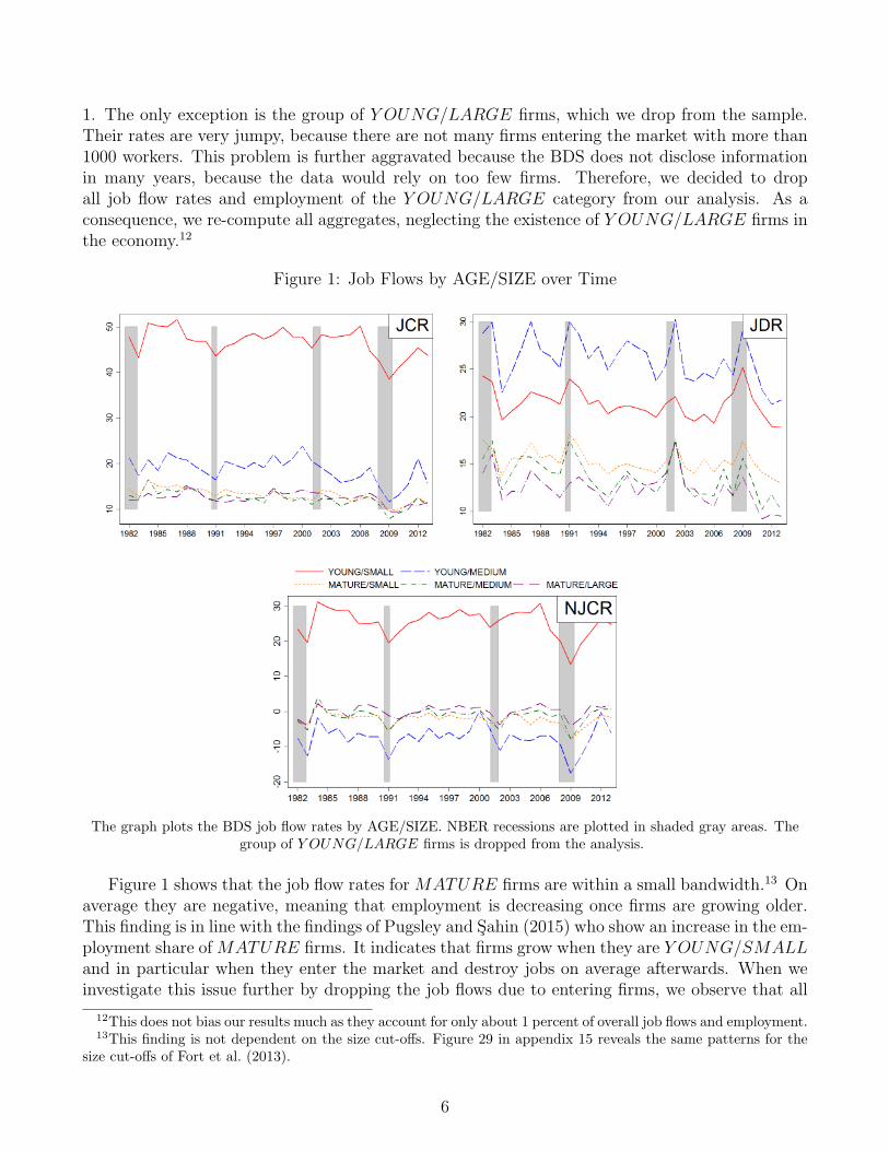
Figure 5: Differential Job Flows during the Great Recession

The graph plots the Differential Job Flows of different groups of firms. From the first top left to bottom rightpanel we look at SIZE, AGE, SIZE conditional on AGE = MATURE, AGE conditional on SIZE = SMALL,and MATURE/LARGE − Y OUNG/SMALL. Differentials are computed by subtracting the respective series.The differentials for JCR, and NJCR can be read in the same way, the one for JDR is consistent when going in

the opposite direction. All series are linearly de-trended.

MATURE. Among MATURE firms no clear difference emerges between MATURE/SMALLand MATURE/LARGE firms. Thus, the result on LARGE firms being cyclically more sensitivethan SMALL firms (Moscarini & Postel-Vinay, 2012) does not hold during the Great Recession.29

The heterogeneous reaction of Y OUNG and MATURE firms is slightly stronger pronounced inthe JCR compared to the JDR.When looking at the contemporaneous correlations of job flow differentials with aggregate GDPand unemployment we get further support for our findings. Table 2 reports the correlation coeffi-cients and their significance level. Even though we base the correlations only on nine observations,many coefficients are statistical significant. The correlations of the SMALL − LARGE differ-ential indicate that SMALL are more sensitive, but with low statistical power. In contrast, theY OUNG − MATURE differential reveals what we have seen in the plots before. Y OUNG arereacting more than MATURE, indicated by the positive correlation with GDP and the negative

29When defining the size cut-off according to Fort et al. (2013) in section 15.1 we verify the results conditionalon MATURE.

15

correlation with unemployment. This result can be found for the results of AGE conditional onSMALL firms in the last column. The correlations of SIZE conditional on MATURE are notsignificant.

Table 2: Contemporaneous Correlations of Differentials with GDP and Unemployment Rate

MATURE : SMALL :SMALL Y OUNG SMALL Y OUNG

−LARGE −MATURE −LARGE −MATURE

JCR GDP 0.34 0.66* -0.38 0.78**(0.38) (0.05) (0.31) (0.01)

U -0.24 -0.51 0.20 -0.54(0.54) (0.16) (0.60) (0.13)

JDR GDP -0.23 -0.60* 0.10 -0.69**(0.55) (0.09) (0.79) (0.04)

U 0.37 0.60* 0.10 0.52(0.33) (0.09) (0.80) (0.15)

NJCR GDP 0.39 0.67* -0.45 0.77**(0.30) (0.05) (0.23) (0.02)

U -0.38 -0.56 0.13 -0.55(0.31) (0.11) (0.74) (0.13)

The table reports correlation coefficients and p-values of differential job flow rates with the cyclical aggregatemeasure (Unemployment Rate or GDP). The differential is computed by simply subtracting the two respective job

flow rates. Data series are linearly de-trended.

3.1.2 Entry and Exit

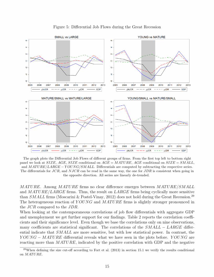
In this section we will document evidence on the behavior of job creation and job destruction atthe entry and exit margin. When interpreting the rates in this section we should keep in mind thatthe definition of the rates deviates from the previous definitions of SIZE and AGE groups. Theusual definition in which we define the job flow by the average employment of a given categorywould yield rates of plus and minus 200 for entry and exit. Therefore, the literature defines theserates in terms of aggregate employment of the economy. When interpreting the job flow rates wecan think of them as weighted rates where the weight is given by the employment share in theeconomy.Before we start analyzing the job flows due to actual entry and exit we will study expanding andcontracting establishments. This will help to better understand the importance of the entry andexit margin as these margins are related to the remaining source of job creation and destruction.The left plot of figure 6 shows the time series of the overall job creation rate and the job creationrate related to the expansion of existing establishments and the setup of new establishments. Thelatter two series add up to the former one by definition. In a similar way, the right graph plotsthe overall job destruction rate of the economy together with the destruction rate of contractingestablishments as well as dead establishments. The figure shows that the lion’s share of job

16

creation and job destruction stems from firms that expand and contract existing establishments.New establishments contribute a smaller share to job creation while the exiting establishmentsalmost do not contribute to the job destruction rate. Surprisingly, the job destruction rate ofexiting establishments seems very flat over time and does not increase much during the GreatRecession. This could be an outcome of policies that were implemented to avoid closure of firms,but also a direct result of lower entry. In normal times the up or out dynamic contributes to thejob destruction. With less entry a drop in exit is therefore an immediate consequence.

Figure 6: Job Creation and Job Destruction during the Great Recession

The left plot shows the JCR broken down by JCREXP and JCRNEW . The right plot shows the JDR brokendown by JDRCONT and JDRDEAD. All rates are linearly de-trended.

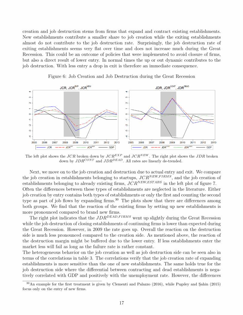
Next, we move on to the job creation and destruction due to actual entry and exit. We comparethe job creation in establishments belonging to startups, JCRNEW,FIRMS, and the job creation ofestablishments belonging to already existing firms, JCRNEW,ESTABS in the left plot of figure 7.Often the differences between these types of establishments are neglected in the literature. Eitherjob creation by entry contains both types of establishments or only the first and counting the secondtype as part of job flows by expanding firms.30 The plots show that there are differences amongboth groups. We find that the reaction of the existing firms by setting up new establishments ismore pronounced compared to brand new firms.

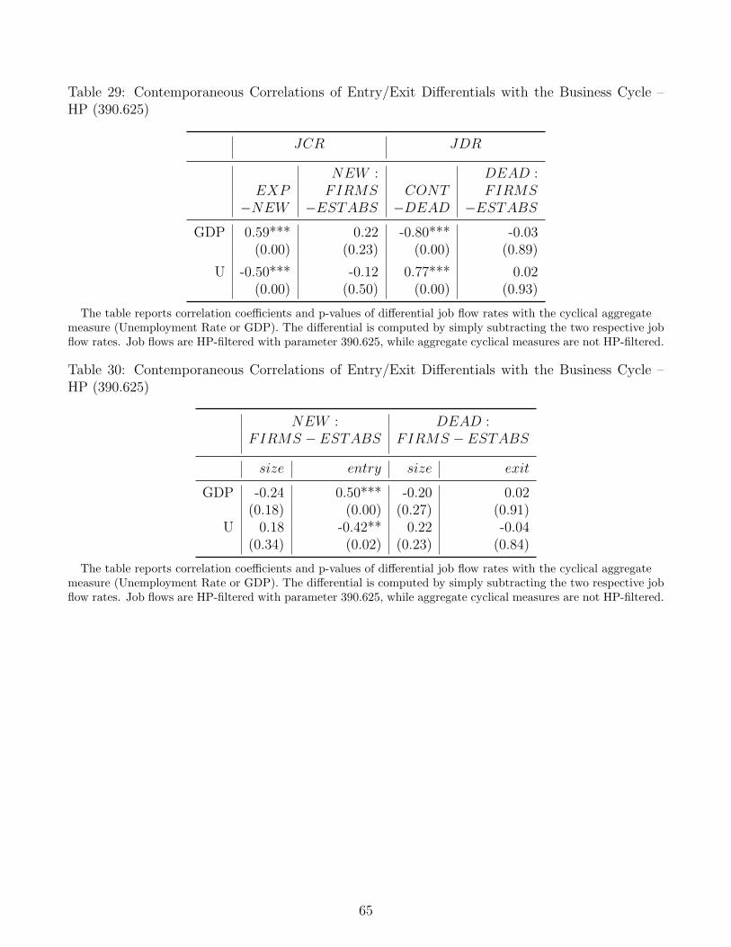
The right plot indicates that the JDRDEAD,FIRMS went up slightly during the Great Recessionwhile the job destruction of closing establishments of continuing firms is lower than expected duringthe Great Recession. However, in 2009 the rate goes up. Overall the reaction on the destructionside is much less pronounced compared to the creation side. As mentioned above, the reaction ofthe destruction margin might be buffered due to the lower entry. If less establishments enter themarket less will fail as long as the failure rate is rather constant.The heterogeneous behavior on the job creation as well as job destruction side can be seen also interms of the correlations in table 3. The correlations verify that the job creation rate of expandingestablishments is more sensitive than the one of new establishments. The same holds true for thejob destruction side where the differential between contracting and dead establishments is nega-tively correlated with GDP and positively with the unemployment rate. However, the differences

30An example for the first treatment is given by Clementi and Palazzo (2016), while Pugsley and Sahin (2015)focus only on the entry of new firms.

17

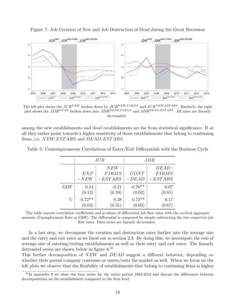
Figure 7: Job Creation of New and Job Destruction of Dead during the Great Recession

The left plot shows the JCRNEW broken down by JCRNEW,FIRMS and JCRNEW,ESTABS . Similarly, the rightplot shows the JDRDEAD broken down into JDRDEAD,FIRMS and JDRDEAD,ESTABS . All rates are linearly

de-trended.

among the new establishments and dead establishments are far from statistical significance. If atall they rather point towards a higher sensitivity of those establishments that belong to continuingfirms, i.e. NEW,ESTABS and DEAD,ESTABS.

Table 3: Contemporaneous Correlations of Entry/Exit Differentials with the Business Cycle

JCR JDR

NEW : DEAD :EXP FIRMS CONT FIRMS

−NEW −ESTABS −DEAD −ESTABS

GDP 0.54 -0.21 -0.76** -0.07(0.13) (0.59) (0.02) (0.85)

U -0.72** 0.38 0.72** 0.17(0.03) (0.31) (0.03) (0.67)



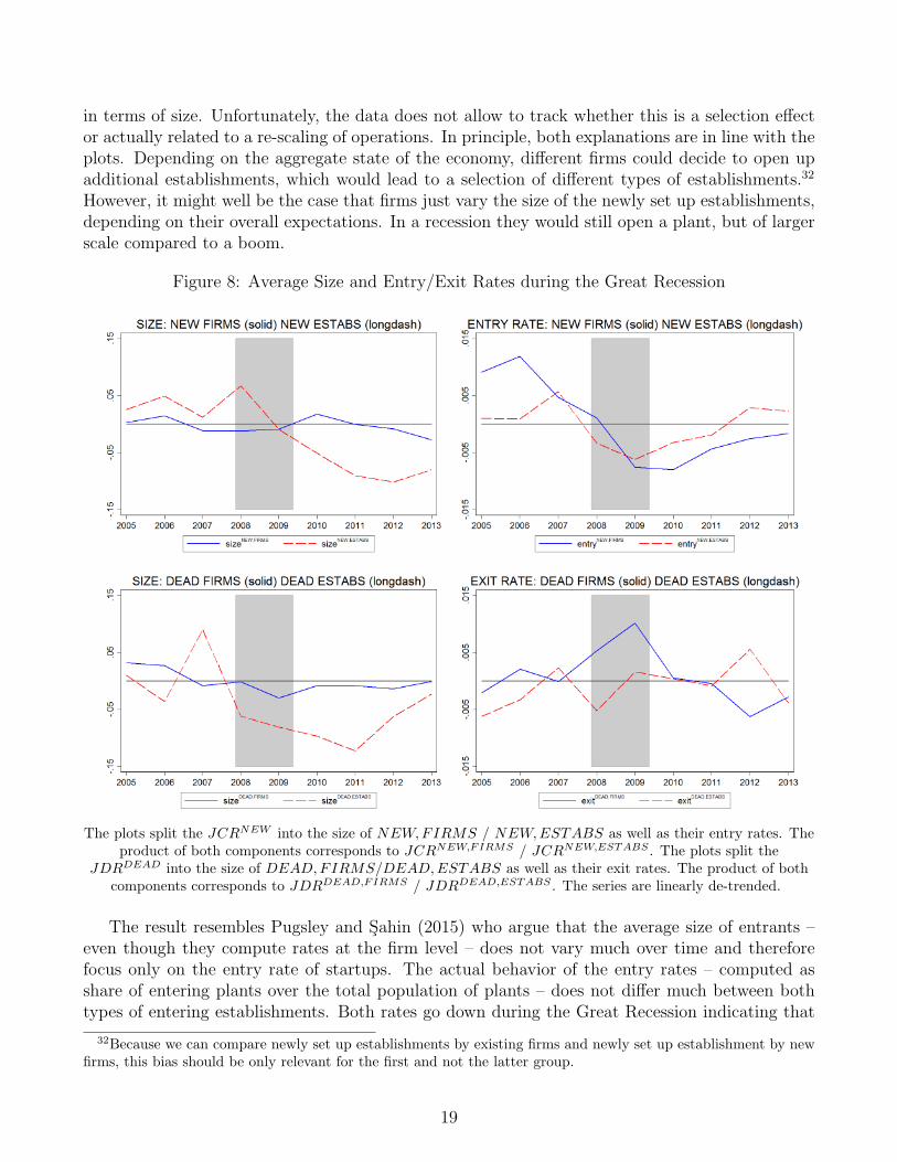
In a last step, we decompose the creation and destruction rates further into the average sizeand the entry and exit rates as we lined out in section 2.3. By doing this, we investigate the role ofaverage size of entering/exiting establishments as well as their entry and exit rates. The linearlydetrended series are shown below in figure 8.31

This further decomposition of NEW and DEAD suggest a different behavior, depending onwhether their parent company continues or enters/exits the market as well. When we focus on theleft plots we observe that the flexibility of establishments that belong to continuing firms is higher

31In appendix 9 we show the time series for the entire period 1982-2013 and discuss the differences betweendecompositions on the establishment compared to the firm level.

18

in terms of size. Unfortunately, the data does not allow to track whether this is a selection effector actually related to a re-scaling of operations. In principle, both explanations are in line with theplots. Depending on the aggregate state of the economy, different firms could decide to open upadditional establishments, which would lead to a selection of different types of establishments.32

However, it might well be the case that firms just vary the size of the newly set up establishments,depending on their overall expectations. In a recession they would still open a plant, but of largerscale compared to a boom.

Figure 8: Average Size and Entry/Exit Rates during the Great Recession

The plots split the JCRNEW into the size of NEW,FIRMS / NEW,ESTABS as well as their entry rates. Theproduct of both components corresponds to JCRNEW,FIRMS / JCRNEW,ESTABS . The plots split the

JDRDEAD into the size of DEAD,FIRMS/DEAD,ESTABS as well as their exit rates. The product of bothcomponents corresponds to JDRDEAD,FIRMS / JDRDEAD,ESTABS . The series are linearly de-trended.

The result resembles Pugsley and Sahin (2015) who argue that the average size of entrants –even though they compute rates at the firm level – does not vary much over time and thereforefocus only on the entry rate of startups. The actual behavior of the entry rates – computed asshare of entering plants over the total population of plants – does not differ much between bothtypes of entering establishments. Both rates go down during the Great Recession indicating that

32Because we can compare newly set up establishments by existing firms and newly set up establishment by newfirms, this bias should be only relevant for the first and not the latter group.

19

less establishments are created. In contrast, the exit rates differ. While the exit of firms goes up,the closure of establishments that belong to continuing firms does not change much.As a last check we look at the actual correlations between the entry/exit rates and average sizewith the aggregate measures. As indicated in table 4 establishments of existing firms react strongerin their size. However, the correlations are not statistically significant. The entry and exit ratesreveal the opposite pattern, i.e. a higher sensitivity of establishments belonging to new or deadfirms. But unfortunately, also these correlations are statistically not significant.


NEW : DEAD :FIRMS − ESTABS FIRMS − ESTABS

size entry size exit

GDP -0.27 0.56 -0.19 -0.11(0.48) (0.11) (0.63) (0.78)

U 0.18 -0.31 0.34 0.22(0.65) (0.41) (0.37) (0.58)



3.2 Contribution to Aggregate Fluctuations in the Great Recession

The previous analysis for the cyclicality of different types of firms during the Great Recession canhelp to understand which firms are hit harder. A potentially more interesting question is howmuch the different groups of firms contribute to the aggregate employment fluctuations during theGreat Recession. The most cyclical firms do not have to be those that contribute most to theaggregate fluctuations in the economy as well. It is a matter of relative and absolute contributionand it turns out that the employment weights are crucial for the contribution to employmentfluctuations. This means that the cyclical analysis does not imply which firms contribute most toaggregate fluctuations during the Great Recession. It might well be that Y OUNG contribute morethan proportional, but the bulk of variance stems from MATURE simply because they representa much larger fraction of employment in the economy. Thus, in this section the overall importanceof the different categories of firms during the Great Recession is evaluated.The approach we use is close to the actual variance decomposition that we described in section2.5. But instead of computing the contribution to the variance of the overall job flows, we simplyexploit the approximation of overall cyclical changes in the job flow into contributions of rates andweights. Because we show in appendix 13 that the variation of the employment weights do not playa role for the cyclical contributions, we only plot the values for the cyclical rates, weighted by theiremployment shares. In this sense we could speak of “weighted” contributions as the deviations ofthe job flows from their linear trend are multiplied by the trend of the employment share, i.e.:

Xt ≈∑

i∈GROUPS

ωitX i

t , (17)

20

where X = {NJCR, JCR, JDR} and GROUPS = {SIZE,AGE,AGE/SIZE}. When wemove to the entry and exit we do not have to additionally weight the rates as they are alreadyweighted. Therefore, those results are in line with the previous findings from the cyclical analysis.


We will start out by investigating the role of the different groups in terms of AGE and SIZEseparately and then discuss the combined AGE/SIZE contributions. Because there are no visibledifferences across the job flow rates we decided to focus only on the NJCR in this section andrefer the interested reader to appendix 11 for the contributions to JCR and JDR.Figure 9 plots the annual contributions to the net job creation rate of AGE (left) and SIZE groups(right). The left plot reveals that the lion’s share of contribution stems from MATURE and notfrom Y OUNG firms. This indicates that the employment weights matter a lot. The results fromthe cyclical analysis showed that the NJCRY OUNG

t is more responsive than the NJCRMATUREt .

Thus by equation (17) we know that the difference in the contributions stems from the employmentweights. Y OUNG firms account to roughly 11 percent of the employment stock, while MATUREfirms employ the remaining workers. This means that even though Y OUNG firms show a strongerreaction during the Great Recession, this behavior is buffered, because of their small employmentshare. In absolute terms their contribution is found to be much less important.33

Figure 9: Contribution to NJCR by AGE and SIZE – Great Recession

The graph plots the weighted contributions of individual job flow rates to overall NJCR. The left plot shows the

contributions broken down by AGE, the right plot is broken down by SIZE. The procedure follows equation

(17).

The right plot of figure 9 in contrast does not show strong heterogeneity for the differentSIZE groups. The bar chart shows that LARGE contributed slightly more to aggregate job flows

33It is important to keep in mind that the contribution we measure here is only related to the direct and immediateeffect. There are additional effects that we do not take into account. For example, less entry and less growth ofY OUNG firms has additional effects when they are supposed to grow older. Pugsley and Sahin (2015) show adirect relation between the decline in the startup rate and the gradual shift of employment towards more maturefirms. Also Sedlacek and Sterk (2014) focus on the impact of recessions for life cycle patterns of firms and aggregateimplications.

21

compared to SMALL.34 The employment shares of the SIZE groups are quite close with SMALL,MEDIUM and LARGE at 29 percent, 27 percent, and 44 percent respectively. Together withthe previous findings that there was no strong difference in terms of the cyclical behavior thisexplains the results.The last decomposition is along the AGE/SIZE dimension at once. Figure 10 shows that amongthe MATURE mainly the LARGE and MEDIUM size firms contribute to overall job flows.Among the Y OUNG it is mainly the SMALL that contribute.

Figure 10: Contribution to NJCR by AGE/SIZE – Great Recession

The graph plots the weighted contributions of individual job flow rates to overall NJCR. The procedure follows

equation (17).

This means that relative and absolute contributions are different for the job flows according toAGE and SIZE. Taking into account the employment weights overturns the cyclical results.


The contributions by entry and exit confirm the cyclical results. Since there is no additionalweighting applied, this section adds mainly to the understanding of the different contributionsover time.Again, we start by studying also those establishments that expand and contract. As shown byfigure 11, the lion’s share of aggregate fluctuations comes from JCREXP and JDRCONT . When

34The results of appendix 15.2, which are based on the cut-offs of Fort et al. (2013) shows a larger contributionof LARGE compared to SMALL, which is mainly a consequence of the smaller employment share for SMALLdue to the different size cut-offs.

22

it comes to entry and exit, it is mainly the entering establishments that contribute to the net jobcreation rate. In particular during the Great Recession the job creation of NEW contributed abigger share, but still not much compared to the contribution of continuing firms. Interestingly,the contribution of JDRDEAD is quite negligible during 2009, meaning that very few jobs weredestroyed because of establishments that actually had to leave the market. This could be an effectof supportive policies that were targeting the survival of firms during the Great Recession.

Figure 11: Contribution to NJCR by Entry and Exit – Great Recession

The graph plots the contribution of JCRNEW , JCREXP , JDRDEAD, and JDRCONT to NJCR. The procedure

follows equation (17). Rates are linearly de-trended.

Next we look at the actual entry and exit of firms and decompose the JCRNEW and JDRDEAD

further into contributions of size and entry/exit rates. We thereby distinguish between the contri-butions that stem from entering and exiting firms, i.e. NEW,FIRMS and DEAD,FIRMS, andcontinuing firms that set up or close establishments, i.e. NEW,ESTABS and DEAD,ESTABS.It can be seen that the role of size of the latter group contributes substantially.The decline of the JCRNEW is partially due to the lower entry rate of new establishments, par-ticularly in 2009. But we observe an additional phenomenon starting from 2009. The average sizeof sizeNEW,ESTABS is declining over the subsequent years, indicating that firms open up smallerplants than before. At the same time this could be an indication that certain frictions make itharder for those firms that want to open up relatively large establishments.One of the reason why the overall JDRDEAD did not contribute much to the NJCR in 2009 isdue to a compositional effect. Although the exit rates of DEAD,FIRMS and DEAD,ESTABSwent up, the overall impact was buffered because the average size of exiting plants was smallerthan usual.

23

Figure 12: Contribution to JCRNEW and JDRDEAD Flows – Great Recession

The graphs decompose the entry, JCRNEW , and exit margin, JDRDEAD, into contributions of size and

entry/exit. The procedure follows equation (17). Rates are linearly de-trended.

3.3 Cyclicality over the Business Cycle

While the previous part focused only on the period of the Great Recession, we now move towardsthe full sample period between 1982 and 2013. The longer sample period allows us to take intoaccount also the 1981/82, 1990/91, and 2001 recession periods and verify our previous findings ina more general context. We focus on heterogeneous cyclical reactions of different groups of firms,similar to Moscarini and Postel-Vinay (2012) and Fort et al. (2013). First, we analyze the SIZEand AGE groups and then investigate the entry and exit of establishments.The longer time series allows us to compute meaningful correlations of differentials with the aggre-gate measures. We will focus on deviations from a linear trend.35 So we measure for instance thecorrelation between the de-trended growth rate of GDP and the differential of the net job creationrate over time:

Corr( ˜log(GDPt), ˜NJCRSMALLt − ˜NJCRLARGE

t ) (18)

Similarly, we will look at differences between various groups on the entry and exit margin.


This section contributes to the discussion on AGE versus SIZE for heterogeneous responses overthe cycle. While Moscarini and Postel-Vinay (2012) highlight the heterogeneous response betweenSMALL and LARGE firms and conclude a higher sensitivity of LARGE firms during periods ofhigh and low unemployment, Fort et al. (2013) put forward the importance of AGE and particularlyY OUNG/SMALL firms.

Based on the BDS data we plot the linearly de-trended job flows in figure 13. NBER recessionsare plotted in shaded gray areas. Starting from the first plot in which we include the overallNJCR, JCR, and JDR, we focus on SMALL and LARGE firms in the middle and Y OUNG

35The main reason of why we de-trend linearly and do not focus simply on the untreated rates is that in some ofthe more disaggregated series we observe trends over time.

24

Figure 13: Job Flows over the Business Cycle

The graph plots the Job Creation Rate of different groups of firms. From the first top left to bottom right panelwe look at SIZE, AGE, SIZE conditional on AGE = MATURE, AGE conditional on SIZE = SMALL, and


and MATURE at the bottom. All plots show a pro-cyclical behavior of the NJCR and the JCR,while JDR behaves counter-cyclical.The graphs allow to compare the behavior across different recessions, the behavior of differentjob flows, and the behavior of different types of firms. While the previously mentioned pro-

25

and counter-cyclicality of the job flows is a general feature that consistently shows up across allrecessions, the magnitudes of cyclical deviations vary across time. A feature of the Great Recessionis that it is the recession with the biggest negative drop in the NJCR over the entire sample period.This is not generally true for the individual JCR and JDR. Other recessions episodes played acrucial role as well. The 2001 recession is the one with the highest peak of the overall JDR andwas particularly harsh for LARGE and MATURE firms. Y OUNG and SMALL were actuallyhit harder on the destruction side during the Great Recession. The drop in the JCR is of similarmagnitude as in the 1981/82 recession, especially for the SMALL and Y OUNG firms.

Figure 14: Differential Job Flows over the Business Cycle

The graph plots the Differential Job Flows of different groups of firms. From the first top left to bottom rightpanel we look at SIZE, AGE, SIZE conditional on AGE = MATURE, AGE conditional on SIZE = SMALL,and MATURE/LARGE − Y OUNG/SMALL. Differentials are computed by subtracting the respective series.The differentials for JCR, and NJCR can be read in the same way, the one for JDR is consistent when going in


To understand the actual differences between SMALL and LARGE, and Y OUNG andMATUREwe plot the differentials in figure 14. Besides plotting the two unconditional differentials in the up-per graphs, we include the SIZE differential conditional on MATURE and the AGE differentialconditional on SMALL at the bottom.For each of these differentials we correlate the differential with the business cycle measure. Sogenerally speaking, each graph corresponds to a correlation coefficient for each job flow differen-

26

tial. In addition to the pure correlation coefficient, the graphs might be interesting to analyzespecific periods of booms and recessions. But in the end the correlation coefficient is our statisticof interest to measure the cyclicality. Therefore, we abstain from plotting all individual graphs forcorrelations with the unemployment rate or GDP and set up a table with correlation coefficientsinstead. In addition to the correlation coefficients, we compute the p-values for the coefficients,which are displayed in parentheses in table 26.


MATURE : SMALL :SMALL Y OUNG SMALL Y OUNG−LARGE −MATURE −LARGE −MATURE

JCR GDP 0.13 0.54*** -0.24 0.69***(0.49) (0.00) (0.19) (0.00)

U -0.15 -0.48** 0.17 -0.58***(0.42) (0.01) (0.35) (0.00)

JDR GDP -0.11 -0.34* -0.03 -0.42**(0.54) (0.06) (0.87) (0.02)

U -0.08 0.19 -0.16 0.38**(0.66) (0.30) (0.39) (0.03)

NJCR GDP 0.19 0.56*** -0.19 0.64***(0.30) (0.00) (0.31) (0.00)

U -0.05 -0.45** 0.30* -0.55***(0.79) (0.01) (0.09) (0.00)



Table 26 reports the correlation coefficients based on linearly de-trended job flow rates. Asshown by the first column, we do not find any statistical support for the result of Moscariniand Postel-Vinay (2012), i.e. LARGE being more sensitive than SMALL related to cyclicalunemployment.36 However, when conditioning on MATURE firms, we find their SIZE result.As seen in column 3, the correlation between the differential NJCR and cyclical unemploymentis 0.30 (p-value 0.09).37

The strongest results, however, are related to AGE. The results in columns 2 and 4 are fully inline with the previous findings for the period of the Great Recession. Y OUNG firms are cyclically

36The results of Moscarini and Postel-Vinay (2012) were found for the period 1979-2009 on a slightly olderversion of the BDS and with HP-filtered aggregate measures. Our codes give a correlation coefficient for the NJCRdifferential and cyclical unemployment of 0.38 (p-value 0.03) for the same period, using the HP filter with parameter390.625, which is in line with their findings. For an extensive discussion of the relation to the results of Moscariniand Postel-Vinay (2012) see appendix 18.

37When we investigated the correlations of the linearly de-trended job flow rates with HP-filtered aggregates onlythe higher cyclical sensitivity of MATURE/LARGE compared to MATURE/SMALL for the JCR and NJCRis found as well.

27

more sensitive than MATURE, indicated for example by the positive correlation of the NJCRdifferential with GDP (0.56).


This section aims to better understand how sensitive job creation and destruction due to entryand exit is over the cycle. Arguments for policies that try to avoid large fluctuations on the entryand exit margin are often mixing up the disproportionate role that entry and exit play in generaland the cyclical role of it.We start again with a wider view and take into account expanding and contracting establishmentsas well. Table 6 reports the differential for EXP −NEW and CONT −DEAD establishments.When focusing on deviations from a linear trend, we find a stronger sensitivity of the establishmentsthat expand and contract.


JCR JDR



GDP 0.58*** 0.15 -0.81*** -0.09(0.00) (0.41) (0.00) (0.61)

U -0.51*** -0.11 0.77*** 0.03(0.00) (0.56) (0.00) (0.88)



Next we investigate differences between those new establishments that belong to brand newfirms and those that are part of continuing firms. The linear de-trending does not indicate anyheterogeneous behavior.Table 7 goes a step further and decomposes the job creation and job destruction rates of NEW andDEAD establishments into the size and entry/exit rates. The results indicate thatNEW,ESTABSreact stronger in terms of establishment size, while NEW,FIRMS show a stronger reaction inthe entry rate. On the destruction side we again find a stronger reaction of DEAD,ESTABS interms of size, but no evidence related to the exit rate.

28


NEW : DEAD :

FIRMS − ESTABS FIRMS − ESTABS


GDP -0.32* 0.51*** -0.31* 0.03(0.07) (0.00) (0.08) (0.88)

U 0.18 -0.41** 0.24 -0.06(0.33) (0.02) (0.19) (0.76)



3.4 Contribution to Aggregate Fluctuations over the Business Cycle

The cyclical sensitivity of different groups of firms that we have documented helps to understandthe relative impact that these groups have. The total impact, however, is strongly related tothe employment share of the individual groups of firms as we have seen for the Great Recession.Therefore, we decompose the variance of aggregate fluctuations into contributions of groups offirms and relate the results with the findings in the Great Recession.38

Pugsley and Sahin (2015) show that the life-cycle dynamics did not change over the period weare investigating. Therefore, changes in the overall employment dynamics are mainly driven bycompositional effect that we take into account by de-trending the variables.We describe the role of AGE and SIZE first and then discuss the contributions that stem fromthe entry and exit of establishments. The results for the Great Recession period are generallyconfirmed.


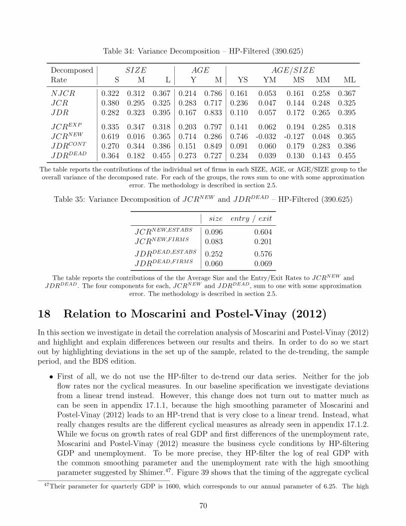
Figure 15 visualizes the contributions of job flow rates of AGE/SIZE groups to overall NJCR.As described in section 2.5 we decompose the NJCR into the AGE/SIZE contributions accordingto JCRNEW , JCREXP , JDRDEAD, and JDRCONT . Therefore, the 20 contributions from figure15 add up to unity with some approximation error.39 The approximation error stems from the factthat we implement a Taylor expansion around the trend. In addition, we neglect the contributionsof cyclical employment weights in this analysis. Those contributions are reported in appendix 13,but are negligible.

Figure 15 shows that the two left plots, i.e. the expansion (34.9 %) and contraction (51.9 %) ofexisting establishments, contribute the lion’s share to aggregate job fluctuations. The destructionside is dominating this decomposition with an overall share of 58.3 %. The plot reveals already

38In principle, cyclical variations can stem from changes of the job flow rates of a group or by compositionalchanges due to changes in the employment weights. We neglect the latter contributions of the weights, becauseweights contribute only a tiny share to aggregate fluctuations as shown in appendix 13. General trends in theemployment weights, however, are taken into account as described by our methodology in section 2.5.

39Remember that we dropped the Y OUNG/LARGE firms from our analysis.

29

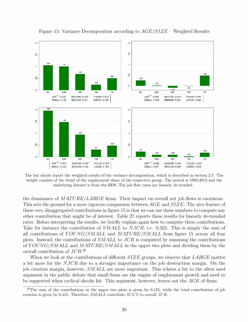
Figure 15: Variance Decomposition according to AGE/SIZE – Weighted Results

The bar charts report the weighted results of the variance decomposition, which is described in section 2.5. Theweight consists of the trend of the employment share of the respective group. The period is 1982-2013 and the

underlying dataset is from the BDS. The job flow rates are linearly de-trended.

the dominance of MATURE/LARGE firms. Their impact on overall net job flows is enormous.This sets the ground for a more rigorous comparison between AGE and SIZE. The nice feature ofthese very disaggregated contributions in figure 15 is that we can use these numbers to compute anyother contribution that might be of interest. Table 27 reports these results for linearly de-trendedrates. Before interpreting the results, we briefly explain again how to compute these contributions.Take for instance the contribution of SMALL to NJCR, i.e. 0.323. This is simply the sum ofall contributions of Y OUNG/SMALL and MATURE/SMALL from figure 15 across all fourplots. Instead, the contributions of SMALL to JCR is computed by summing the contributionsof Y OUNG/SMALL and MATURE/SMALL in the upper two plots and dividing them by theoverall contribution of JCR.40

When we look at the contributions of different SIZE groups, we observe that LARGE mattera bit more for the NJCR due to a stronger importance on the job destruction margin. On thejob creation margin, however, SMALL are more important. This relates a bit to the often usedargument in the public debate that small firms are the engine of employment growth and need tobe supported when cyclical shocks hit. This argument, however, leaves out the AGE of firms.

40The sum of the contributions in the upper two plots is given by 0.155, while the total contribution of jobcreation is given by 0.415. Therefore, SMALL contribute 37.3 % to overall JCR.

30

Table 8: Variance Decomposition of Job Flows

Decomposed SIZE AGE AGE/SIZERate S M L Y M YS YM MS MM ML

NJCR 0.323 0.311 0.367 0.216 0.784 0.162 0.054 0.160 0.257 0.367JCR 0.373 0.292 0.335 0.284 0.716 0.234 0.051 0.140 0.241 0.335JDR 0.286 0.324 0.389 0.168 0.832 0.111 0.057 0.175 0.268 0.389

The table reports the contributions of the individual set of firms in each SIZE, AGE, or AGE/SIZE group tothe overall variance of the decomposed rate. For each of the groups, the rows sum to one with some

approximation error. The methodology is described in section 2.5.

Comparing Y OUNG and MATURE firms reveals a very clear picture that MATURE contributearound three quarters to the overall cyclical job flows. This is not surprising as MATURE firmsemploy about 85 percent of the overall workforce. Thus, it is quite natural that they play a crucialrole for the overall job flows. Again, we observe differences on the job creation and destructionmargin. While MATURE contribute 83.2% to the JDR, they contribute substantially less toJCR with 71.6%.The last five columns of the table show the contributions of all AGE/SIZE categories. AmongY OUNG mainly Y OUNG/SMALL contribute to cyclical fluctuations. They contribute a verydisproportional share to the cyclicality of overall job flows. In terms of individual groups that con-tribute most to aggregate fluctuations, we can see thatMATURE/LARGE andMATURE/MEDIUMplay a crucial role and in sum matter for more than half of the overall cyclical job flows.An important point, however, that the decomposition illustrates is that policies that might helpSMALL and in particular Y OUNG/SMALL can obviously have a disproportionate effect on theoverall cyclicality of job flows, but are limited at the same time. Overall, any policy tool thatsupports for instance Y OUNG/SMALL is limited to affect a small fraction of overall net jobcreation, while a policy that targets large mature firms can act on a much larger share of thecyclical NJCR. Thus, this exercise helps to better understand the angle that policies are workingon and their limitations when it comes to the stabilization of overall employment fluctuations.In a last step, we compute “unweighted” contributions. This will highlight the relative contribu-tion as it takes into account the employment weights. We divide the “weighted” contributions byaverage employment shares over the period, reported in table 9.41

Figure 16 plots the unweighted contributions of the different AGE/SIZE groups. The plotsshow the crucial role of Y OUNG/SMALL businesses at the entry and exit margin and Y OUNGfirms in general. The actual numbers do not have a precise meaning, but can be interpreted asrelative contributions compared to other categories. The results also relate to the standard devi-ations for the de-trended rates. Those categories with a higher relative contribution to aggregatevolatility feature higher standard deviations for their de-trended rates as well.

41A problem that we face in this respect is that we can only divide by the average employment share andtherefore might face a bias. Since the cyclical behavior did not change significantly over time as found by Pugsleyand Sahin (2015), we do not face a general problem with the variance decomposition. However, when dividing bythe employment share of LARGE firms, for instance, we will over-state the importance at the beginning and under-state the importance towards the end of the period. Similarly for groups that faced a decrease in the employmentshare over time we will face the opposite pattern.

31

Table 9: Average Employment Weights

Y OUNG MATURESMALL MEDIUM SMALL MEDIUM LARGE

Employment Share 10.4% 3.7% 20.5% 23.1% 42.3%

The table reports the average employment shares of the firm groups in the economy over the period 1982-2013.Young Large firms were completely dropped from the analysis and therefore do not contribute to overall

employment.

Figure 16: Variance Decomposition according to AGE/SIZE – Unweighted Results

The bar charts report the results of the variance decomposition, which is described in section 2.5. The period is1982-2013 and the underlying dataset is from the BDS. The job flow rates are linearly de-trended. Actual

contributions are unweighted as the weighted contributions are divided by the average employment share over theobservation period, shown in table 9.


The job creation and job destruction of NEW and DEAD as well as EXP and CONT establish-ments are reported in table 10. We have seen already from figure 15 that the margin of expansionand contraction plays a more important role than the actual entry and exit.In general MATURE firms are dominating the decomposition with a contribution that is aroundfour times higher than the one of Y OUNG firms. The only exception where the pattern is reversedis the JCRNEW .

32

When it comes to SIZE the expansion and contraction of existing establishments is quite evenlycaused by all three size categories. In contrast, the opening and closing of new establishmentsis dominated by one group. While SMALL are responsible for about three quarters of overallcyclical JCRNEW , about half of the JDRDEAD is due to LARGE.

Table 10: Variance Decomposition of Job Flows at Entry/Exit Margin


JCREXP 0.335 0.347 0.318 0.206 0.794 0.143 0.063 0.192 0.284 0.318JCRNEW 0.576 0.000 0.424 0.697 0.303 0.712 -0.015 -0.136 0.015 0.424JDRCONT 0.270 0.343 0.387 0.150 0.850 0.091 0.060 0.179 0.283 0.387JDRDEATH 0.422 0.172 0.406 0.313 0.688 0.281 0.031 0.141 0.141 0.406



Next we decompose the JCRNEW and the JDRDEAD further into contributions of size andentry/exit rates. The results of the linearly de-trended rates confirm what we observed for theperiod of the Great Recession. Continuing firms are more flexible when it comes to adjustingthe size of new establishments and closing establishments. The size of JCRNEW,ESTABS andJDRDEAD,ESTABS contributed significantly to overall fluctuations. In addition, most of the con-tribution to the overall rates is caused by NEW and DEAD establishments of continuing firms.The actual entry and exit of firms contributes mainly through the entry and exit rate as arguedby Pugsley and Sahin (2015).

Table 11: Variance Decomposition of JCRNEW and JDRDEAD

Decomposed Rate size entry / exit

JCRNEW,ESTABS 0.198 0.506JCRNEW,FIRMS 0.098 0.208

JDRDEATH,ESTABS 0.355 0.468JDRDEATH,FIRMS 0.076 0.068

The table reports the contributions of the the Size and the Entry/Exit Rates to JCRNEW and JDRDEAD. The

four components for each, JCRNEW and JDRDEAD, sum to one with some approximation error. The

methodology is described in section 2.5.

33

4 Discussion of Policies

Discussing policies on small and large firms is a highly controversial field in the political domain.The accusations and arguments start already with defining the “right” measurement of the eco-nomic importance of small businesses and the frictions that affect them. Some policy research evendemands the end of all subsidies to small businesses (Rugy, 2005). At the same time, ongoing dis-cussions about the impact of political lobbying or the recent focus on tax evasion of multi-nationalenterprises are related to large corporations. It is argued that policy-makers care too much aboutbig businesses and do not acknowledge the importance of small businesses.We want to contribute to this discussion by giving a brief overview of current policies in place andrelating them to our empirical findings. By doing so we cannot challenge any results related to theinnovative capacities of certain groups of firms or their overall contribution to economic growth.Instead we add to the discussion by providing information on the role of different groups of firmsfor the cyclical behavior of job flows.An important information to start with is that it is very different what we describe as small andwhat the political process defines as small. For many industries the threshold of small businessesis set to 500 workers by the Small Business Administration (SBA) and therefore much higher thanour size cut-off.The general belief of advocates of small firms is that these small firms are the engines of (job)growth and the place in which most of innovation takes place.42 Often mentioned examples are ITcompanies starting in garages, such as Google or Apple, and then heavily innovate and create jobsand value over time. But due to frictions not enough resources are allocated to these small firms.Potential frictions are the access to credit, externalities of technological spill-overs that are notinternalized, and fixed costs due to regulations. That not all small firms are necessarily Google orApple and could be also the entry of a real estate agent, the coffee shop around the corner, or theopening of a new barber shop is often downplayed.There are several policies in place to support small businesses in the United States.43 Many ofthose are taken care of by the SBA. In general they could be classified into direct and indirectsubsidies.The direct subsidies relate mainly to SBA programs related to the supply of credits. To facilitatethe access to credits and help the liquidity constrained firms, the SBA allows credits to smallbusinesses. Other forms of supporting small businesses are preferential treatments. Smaller firmsare exempted from taxation or face tax breaks. Many of the regulatory burden is given to biggerfirms, trying to lower the fixed costs of very small businesses by exempting them from certainrequirements. A non negligible amount of direct spending of public procurement on small firmsis also required by law. During the Great Recession various direct policies were implemented tosupport small businesses. By giving tax cuts to small businesses and increasing their access tofinance, these policies should help to dampen the negative shock to small businesses during theGreat Recession.44 The aim of these policies is to fuel the credit supply to small businesses by

42That this view on small businesses might have to be revised can be seen from research by Hurst and Pugsley(2011). Based on surveys they find that most small business owners do not have the intention to grow big, butrather serve an existing market with an existing product or service. This questions also the idea of small businessesbeing the cradle of innovation.

43A brief overview of different policies with exact criteria can be found in the discussion of Adam Looney in Hurstand Pugsley (2011).

44Policies were for example the “Small Business Jobs Act” in 2010, the “Hiring Incentives to Restore Employment(HIRE) Act” in 2010, the “Middle Class Tax Relief and Job Creation Act” in 2012. The “Red Tape Reduction and

34

giving government-backing for a fraction of the loans that partner banks give to these businesses.The indirect subsidies are mainly non-pecuniary benefits. And they are generally not taxed. Forexample, small business owners can benefit from being their own boss and have more flexibleworking hours. There is also evidence that small business owners under-report their income to taxauthorities (Hurst, Li, & Pugsley, 2010).All these aforementioned subsidies are often linked to firm size, based on head-count measuresof workers. This could actually inhibit growth by causing new distortions. Firms face additionalcosts when crossing these size thresholds. Therefore, they might prefer to stay slightly below thethreshold and still be eligible to receive certain subsidies instead of growing to their optimal size.But there is also a more fundamental problem with these policies. It seems that many policies areactually set up in the mindset of supporting firms that face frictions when growing or are negativelyimpacted by aggregate shocks. Whether policies should therefore relate to size or age is not clear.There is little empirical evaluation available to study the effectiveness of current policies. By im-precise targeting, new distortions could arise. Our analysis revealed that the usual size distinctionis not the relevant margin for business cycle fluctuations of job flows. Instead, the age of firms isfound to be a more relevant margin, independent of size. Young firms are more cyclically sensitiveto aggregate fluctuations. Thus, it seems to be a more relevant margin to include the firm age aswell.For policies that target the stabilization of aggregate employment over the business cycle our re-sults from the variance decomposition analysis are relevant.45 While young firms are more sensitiveto the cycle, they contribute only very little to overall fluctuations. During the Great Recessionthey caused roughly around 20 percent of overall fluctuations. Thus, policies supporting the jobs inmature firms can have more leverage as more than 80 percent of employment is in mature firms.46

5 Conclusion

This paper investigates the cyclical behavior of heterogeneous firms in their job flows and theircontribution to employment fluctuations. Of particular interest are firms of different size and ageas well as the entry and exit margin. The first part of the analysis focuses on the period of theGreat Recession, while the second investigates the behavior over multiple business cycles between1982-2013.For the period of the Great Recession we document important heterogeneity along the dimensionof firm age. We find that firms younger than 5 years are hit harder than mature firms. Wheninvestigating the role of firm size, we do not find evidence of a heterogeneous behavior of small andlarge firms in contrast. However, when measuring the actual contribution to overall employmentfluctuations the findings revert. Because of their small employment share, young firms contributerelatively little to overall employment fluctuations. Instead, mature firms contribute the lion’sshare.For the period from 1982-2013 results are more dependent on the data treatment. Linearly de-trended job flows confirm our findings for the Great Recession and show that young firms are more

Small Business Job Creation Act” of 2012 is a law that puts a stronger emphasis on the regulatory costs for smallbusinesses. The act tries to reduce regulations for small businesses to make it easier for them to hire new workers.

45Note that in principle job losses due to aggregate fluctuations could be an efficient outcome as well if they arecleansing.

46The results of our variance decomposition are only based on direct effects, while there might well be additionaldynamic effect that accumulate over time as shown by Sedlacek and Sterk (2014).

35

sensitive than mature firms.In general, we find the job creation and destruction due to actual entry and exit of establishmentsrelatively less important compared to the expansion and contraction of existing establishments.Our findings underline the importance of firm age for policies and general discussions on cyclicaleffects on heterogeneous firms. As shown, most policies are centered around the size dimension offirms. The conventional view of economists and policymakers sees small businesses as the engine ofgrowth with an important role for job creation and innovation. The cyclical sensitivity, however, isstronger related to firm age than to firm size. Therefore, it could be instructive to shift the focusmore towards the role of small and young firms instead of only small.This study also questions the argument of granularity, i.e. large firms driving the cycle, on thebasis of cyclical job flows. Taking the granular argument literally, we would not only see thatlarge firms are stronger correlated with the business cycle, but also that – as long as there is nofurther amplification – large firms contribute disproportionately to the aggregate fluctuations (asthey are partially caused by them). While we confirm the findings of Moscarini and Postel-Vinay(2012) that large firms are more sensitive to the cycle, we can definitely rule out that large firmscontribute disproportionally to aggregate fluctuations. Our variance decomposition shows thatlarge and mature firms contribute the lion’s share to aggregate fluctuations, but this is mainly dueto their large share in overall employment. Nevertheless, they contribute relatively less comparedto small and young firms.

36

References

Clementi, G. L., & Palazzo, D. (2016). Entry, Exit, Firm Dynamics, and Aggregate Fluctuations.American Economic Journal: Macroeconomics , forthcoming.

Davis, S., Haltiwanger, J. C., & Schuh, S. (1996). Job Creation and Destruction. MIT Press.Fort, T. C., Haltiwanger, J., Jarmin, R. S., & Miranda, J. (2013). How Firms Respond to Business

Cycles: The Role of Firm Age and Firm Size. IMF Economic Review , 61 (3), 520–559.Hurst, E., Li, G., & Pugsley, B. (2010). Are Household Surveys Like Tax Forms: Evidence from

Income Underreporting of the Self Employed (NBER Working Paper No. 16527). NationalBureau of Economic Research, Inc. 2016-01-30

Hurst, E., & Pugsley, B. W. (2011). What do Small Businesses Do? Brookings Papers on Economic

Activity , 43 (2 (Fall)), 73–142.Moscarini, G., & Postel-Vinay, F. (2012). The Contribution of Large and Small Employers to Job

Creation in Times of High and Low Unemployment. American Economic Review , 102 (6),2509–39.

Pugsley, B. W., & Sahin, A. (2015). Grown-Up Business Cycles (Working Paper No. 15-33).Center for Economic Studies, U.S. Census Bureau. 2016-01-30

Rugy, V. d. (2005). Are Small Businesses the Engine of Growth? (Working Paper No. 49882).American Enterprise Institute. 2016-01-26

Sedlacek, P., & Sterk, V. (2014). The Growth Potential of Startups over the Business Cycle

(Discussion Paper No. 1403). Centre for Macroeconomics (CFM). 2016-01-30

37

6 Distribution of Job Creation and Destruction across Firm

Groups

To better understand how job creation and destruction is divided across firms, we include thefollowing table. It reports the average shares of job creation and destruction shares due to varioussize and age categories. The last row reports the shares of small young firms without the newentrant firms.

Table 12: Average Job Creation and Job Destruction Shares of Different Groups

JOB CREATION JOB DESTRUCTIONNEW EXP TOTAL DEAD CONT TOTAL

Y OUNG .53 .22 .34 .31 .16 .21MATURE .46 .78 .66 .69 .84 .79

Y OUNG/SMALL .50 .17 .29 .23 .11 .15Y OUNG/MEDIUM .03 .05 .04 .08 .05 .06MATURE/SMALL .05 .23 .16 .22 .21 .21MATURE/MEDIUM .12 .21 .17 .18 .23 .21MATURE/LARGE .30 .34 .33 .29 .40 .36

Y OUNG/SMALLwithout Firm Entry .03 .17 .12 .23 .11 .15

The table reports the average shares for job creation and destruction as share of the respective column. Theunderlying data stems from the BDS and the period covers 1982-2013. The last row re-computes the average

shares for Y OUNG/SMALL firms, deducting the job creation caused by firm entry.

As can be seen from the second line of the table 12, MATURE create (66 percent) and destroy(79 percent) the bulk of all jobs. Most of this creation (74 percent) and destruction (70 percent)of MATURE stems from the intensive margin, i.e. expansion and contraction of already existingestablishments, as seen in table 13. In contrast, the creation and destruction shares for Y OUNGare almost balanced between the intensive margin – expanding/contracting existing establishments(42 percent / 50 percent) – and the extensive margin – opening/closing establishments (58 percent/ 50 percent).Next, we can look at the shares of different AGE/SIZE groups. For the job creation, mainlyMATURE/LARGE (33 percent) and Y OUNG/SMALL (29 percent) are important, while forthe job destruction MATURE/LARGE (36 percent), MATURE/MEDIUM (21 percent), andMATURE/SMALL (21 percent). The margins of adjustment of table 13 are different acrossSIZE groups. For job creation, with around 34 percent LARGE firms adjust more on the ex-tensive margin compared to medium (around 25 percent) and small firms (around 10 percent).In contrast, the extensive margin plays a more important role for job destruction at particularY OUNG/SMALL (52 percent) and Y OUNG/MEDIUM (44 percent).

In addition to the figures that are visible in the table, we looked into the entry and exit offirms as well. The job creation of new born firms represents 18 percent of total job creation and47 percent of all jobs created by newly created establishments. Similarly, 48 percent of all jobsdestroyed through establishments closing are due to firm closure. 17 percent of all destroyed jobs

38

Table 13: Distribution of Job Creation and Job Destruction across Extensive and Intensive Margins

JOB CREATION JOB DESTRUCTIONNEW EXP DEAD CONT

TOTAL

Y OUNG .58 .42 .50 .50MATURE .26 .74 .30 .70

Y OUNG/SMALL .63 .37 .52 .48Y OUNG/MEDIUM .26 .74 .44 .56MATURE/SMALL .12 .88 .36 .64MATURE/MEDIUM .25 .75 .29 .71MATURE/LARGE .34 .66 .28 .72

Y OUNG/SMALLwithout Firm Entry .09 .91 .52 .48

The table reports the distribution of job creation and job destruction across new/expanding anddying/contracting firms respectively. The underlying data stems from the BDS and the period covers 1982-2013.

are caused by exiting firms. In terms of firm age, Y OUNG and MATURE exiting firms contributeequally to job destruction. LARGE do not matter much as exit of LARGE is a very rare event.Jobs are mainly destroyed by SMALL. The individual contributions to overall job destruction aregiven by Y OUNG/SMALL (6 percent), MATURE/SMALL (6 percent), Y OUNG/MEDIUM(2 percent), and MATURE/MEDIUM (3 percent).

39

7 BDS Employment Shares over Time

A glance at the time series shows that the employment share of large firms is constantly increasingover time, while the share of small firms is decreasing. Pugsley and Sahin (2015) show that theincrease in employment of LARGE – and particularly MATURE/LARGE – firms is likely aconsequence of a decline in the startup rate.Besides these obvious trends in the data, there is a visible cyclicality in the employment shares.When focusing only on the NBER recession periods, shaded in gray, the importance of large firmsfor the aggregate employment seems to increase, while the one for small firms decreases.

Figure 17: Employment Share by SIZE

The gray lines represent the HP-trends of the data series. The shaded gray areas represent NBER recession

periods. Data stems from the BDS.

Even though, employment shares shifted towards more mature and large firms, one can observefrom the following graphs that employment of all firm sizes increased during the observed period.So the decline of small firms is only a relative trend.

Figure 18: Employment Levels by SIZE

Employment is measured in thousands of workers. Data stems from the BDS.

40

The employment shares of different AGE/SIZE groups seems more stable over time, butreveals opposing trends for young and mature firms. Between 1982 and 2013 the employmentshare of young firms decreased from overall 19.1 percent to 10.2 percent. Most of this change isdue to a decline of employment in Y OUNG/SMALL, which decreased from 13.6 percent to 7.3percent, which is related to a decline in entry as well as average entry size over time. All thesefindings are in line with Pugsley and Sahin (2015), even though they use a different size and agecut-off.

Figure 19: Employment Share by AGE/SIZE

The gray lines represent the HP-trends of the data series. The shaded gray areasrepresent NBER recession periods. Data stems from the BDS.

41

8 Job Flows without Firm Entry

This section is plotting the three different job flow rates over time, neglecting the existence of firmentry, i.e. 0 age firms from the BDS dataset. Obviously, the JDR is identical with the one shownin figure 1 in the main text. The JCR of Y OUNG/SMALL, however, is dropping strongly. Thisunterlines the importance of the entry margin for the job creation. However, these plots onlydescribe the behavior of job flow rates over time and do not indicate the cyclicality, which is ourresearch focus.

Figure 20: Job Flow Rates by AGE/SIZE over Time without Firm Entry


42

9 Entry/Exit at the Firm Level

In this section we plot the decomposition of the the job creation and destruction rate of new firmson the firm level, similar to Pugsley and Sahin (2015). The plots show that the pattern of entryand exit rates as well as size is the same for the firm and establishment level. Only the size differsslightly, because the number of establishments of new firms is larger than the number of new firmsitself and the same for exiting firms.The job creation rate of new firms is decomposed into the firm entry rate and the relative firmsize:

JCRNEW,FIRMSt =

#FIRMSNFt

#FIRMSt︸︷︷︸Firm Entry Rate NF

×

JCNFt

#FIRMSNFt

EMPt

#FIRMSt︸︷︷︸Relative Firm Size NF

(19)

Figure 21: Decomposing JCRNEW,FIRMS on the Firm and Establishment Level

The graph shows the relative firm and establishment size as well as the firm and establishment entry rates. The

vertical line in 2009 represents the trough of the Great Recession.

Similarly, the job destruction rate of dying firms is decomposed into the firm exit rate and therelative firm size:

JDRDEAD,FIRMSt =

#FIRMSDFt

#FIRMSt︸︷︷︸Exit Rate DF

×

JDDFt

#FIRMSDFt

EMPt

#FIRMSt︸︷︷︸Relative Firm Size DF

(20)

43

Figure 22: Decomposing JDRDEAD,FIRMS on the Firm and Establishment Level

The graph shows the relative firm and establishment size as well as the firm and establishment entry rates. The

vertical line in 2009 represents the trough of the Great Recession.

44

10 Differential Job Flows during the Great Recession –

Alternative Filters

Figure 23: Differential Job Flows during the Great Recession – Alternative Filters

Linear Trend De-Meaned HP-filtered (390.625)

45

11 Contributions to JCR and JDR during the Great Re-

cession

Figure 24: Contribution to JCR and JDR by SIZE – Great Recession

The graph plots the weighted contributions of individual job flow rates to overall JCR and JDR. The procedure

follows equation (17).

Figure 25: Contribution to JCR and JDR by AGE – Great Recession



46

Figure 26: Contribution to JCR and JDR by AGE/SIZE – Great Recession



In addition, we decompose the variance as outlined in section 2.5 even though we base theanalysis on only nine data points.

Table 14: Variance Decomposition – Great Recession


NJCR 0.322 0.307 0.371 0.203 0.797 0.155 0.048 0.167 0.259 0.371JCR 0.342 0.304 0.354 0.239 0.761 0.190 0.049 0.152 0.255 0.354JDR 0.302 0.310 0.387 0.168 0.832 0.121 0.047 0.182 0.263 0.387

JCREXP 0.267 0.350 0.383 0.152 0.848 0.096 0.055 0.171 0.295 0.383JCRNEW 0.550 0.176 0.275 0.481 0.519 0.450 0.031 0.099 0.145 0.275JDRCONT 0.269 0.350 0.381 0.132 0.868 0.081 0.051 0.187 0.299 0.381JDRDEATH 1.400 -1.000 0.600 1.333 -0.333 1.400 -0.067 0.000 -0.933 0.600

The table reports the contributions of the individual set of firms in each SIZE, AGE, or AGE/SIZE group to

the overall variance of the decomposed rate. For each of the groups, the rows sum to one with some


47

Table 15: Variance Decomposition of JCRNEW and JDRDEAD – Great Recession

size entry / exit

JCRNEW,ESTABS 0.005 0.632JCRNEW,FIRMS -0.037 0.386

JDRDEATH,ESTABS 0.542 0.649JDRDEATH,FIRMS -0.232 -0.008

The table reports the contributions of the the Size and the Entry/Exit Rates to JCRNEW and JDRDEAD. Thefour components for each, JCRNEW and JDRDEAD, sum to one with some approximation error. The

methodology is described in section 2.5.

48

12 Differential Job Flows over the Business Cycle – Alter-

native Filters

Figure 27: Differential Job Flows over the Business Cycle – Alternative Filters

Linear Trend De-Meaned HP-filtered (390.625)

49

13 Contribution of Employment Weights to Variance De-

composition

Figure 28: Variance Decomposition according to AGE/SIZE – Weighted Results for Weights

The bar charts report the weighted results of the variance decomposition, which is described in section 2.5. The

weight consists of the trend of the NJCR of the respective group. The period is 1982-2013 and the underlying

dataset is from the BDS. The job flow rates are linearly de-trended.

50

14 Robustness – HP-Filtered Aggregates

In this section we investigate the correlation patterns between linearly de-trended job flow ratesand HP-filtered aggregate measures.




JCR GDP 0.00 0.07 -0.28 0.20(0.98) (0.71) (0.13) (0.28)

U 0.15 0.13 0.32* -0.01(0.41) (0.48) (0.08) (0.95)

JDR GDP 0.22 0.10 0.20 -0.02(0.23) (0.60) (0.27) (0.91)

U -0.16 -0.16 -0.12 -0.14(0.38) (0.37) (0.53) (0.45)

NJCR GDP -0.17 0.01 -0.44** 0.17(0.34) (0.94) (0.01) (0.37)

U 0.25 0.17 0.39** 0.03(0.17) (0.36) (0.03) (0.88)

The table reports correlation coefficients and p-values of differential job flow rates with the cyclical aggregatemeasure (Unemployment Rate or GDP). The differential is computed by simply subtracting the two respective jobflow rates. Job flow rates are linearly de-trended, GDP (parameter 6.25) and the unemployment rate (parameter

390.625) are HP-filtered.


JCR JDR



GDP -0.03 -0.28 -0.27 -0.01(0.89) (0.12) (0.13) (0.94)

U 0.16 0.39** 0.06 0.04(0.38) (0.03) (0.73) (0.83)



51




GDP -0.09 -0.04 0.04 -0.06(0.61) (0.81) (0.82) (0.75)

U 0.15 0.14 0.01 0.01(0.41) (0.44) (0.95) (0.96)



52

15 Robustness – Alternative Size Cut-off

While we follow Moscarini and Postel-Vinay (2012) in defining small, medium, and large firms,Fort et al. (2013) as well as Pugsley and Sahin (2015) use different size cut-offs. Compared to ourdefinition (small: less than 50; medium: 50-1000; large: more than 1000), we apply the alternativesize cut-off in this section (small: less than 20; medium: 20-500; large: more than 500).Note that the aggregate job flow rates are the same as in the baseline case, i.e. all values fromfirms with more than 1000 employees and less than 5 years of age are dropped from the sample.Thus, the category of young large firms is only composed of young firms with 500-1000 employees.

Figure 29: Job Flow Rates by AGE/SIZE over Time – Alternative Size Cut-off


53

15.1 Cyclicality in the Great Recession

Figure 30: Job Creation Rate during the Great Recession

The graph plots the Job Creation Rate of different groups of firms. From the first top left to bottom right panel

we look at SIZE, AGE, SIZE conditional on AGE = MATURE, AGE conditional on SIZE = SMALL, and


54

Figure 31: Differential Job Flows during the Great Recession

The graph plots the Differential Job Flows of different groups of firms. From the first top left to bottom right

panel we look at SIZE, AGE, SIZE conditional on AGE = MATURE, AGE conditional on SIZE = SMALL,

and MATURE/LARGE − Y OUNG/SMALL. Differentials are computed by subtracting the respective series.

The differentials for JCR, and NJCR can be read in the same way, the one for JDR is consistent when going in


55

Figure 32: Job Creation and Job Destruction during the Great Recession by Entry and Exit

The plots show the job creation and destruction rates by expanding/contracting establishments of existing firms,

new or dying establishments of continuing firms, and new or dying establishments of those firms that enter or exit

the market. All rates are linearly de-trended.

15.2 Contribution to Aggregate Fluctuations in the Great Recession

Figure 33: Contribution to Job Flows by SIZE – Great Recession

The graph plots the weighted contributions of individual job flow rates to overall JCR, JDR, and NJCR

respectively. The procedure follows equation (17).

56

Figure 34: Contribution to Job Flows by AGE/SIZE – Great Recession

The graph plots the weighted contributions of individual job flow rates to overall JCR, JDR, and NJCR

respectively. The procedure follows equation (17).


Table 19: Contemporaneous Correlations of Differentials with GDP and Unemployment Rate –Alternative Size


JCR GDP 0.18 0.54*** -0.31* 0.65***(0.32) (0.00) (0.09) (0.00)

U -0.14 -0.48** 0.30 -0.58***(0.44) (0.01) (0.10) (0.00)

JDR GDP -0.00 -0.34* 0.11 -0.54***(1.00) (0.06) (0.54) (0.00)

U -0.17 0.19 -0.28 0.49***(0.35) (0.30) (0.13) (0.00)

NJCR GDP 0.13 0.56*** -0.34* 0.64***(0.46) (0.00) (0.06) (0.00)

U 0.02 -0.45** 0.47** -0.57***(0.93) (0.01) (0.01) (0.00)


flow rates. Data series are either linearly de-trended or HP-filtered with parameter 6.25.

57

Table 20: Contemporaneous Correlations of Entry/Exit Differentials with the Business Cycle –Alternative Size

JCR JDR



GDP 0.58*** 0.15 -0.81*** -0.09(0.00) (0.41) (0.00) (0.61)

U -0.51*** -0.11 0.77*** 0.03(0.00) (0.56) (0.00) (0.88)




NEW : DEAD :

FIRMS − ESTABS FIRMS − ESTABS


GDP -0.32* 0.51*** -0.31* 0.03(0.07) (0.00) (0.08) (0.88)

U 0.18 -0.41** 0.24 -0.06(0.33) (0.02) (0.19) (0.76)



58


Figure 35: Variance Decomposition according to AGE/SIZE – Weighted Results


weight consists of the trend of the employment share of the respective group. The period is 1982-2013 and the

underlying dataset is from the BDS. The job flow rates are Linearly De-Trended.

59

Figure 36: Variance Decomposition according to AGE/SIZE – Unweighted Results

The bar charts report the results of the variance decomposition, which is described in section 2.5. The period is

1982-2013 and the underlying dataset is from the BDS. The job flow rates are Linearly De-Trended. Actual

contributions are unweighted as the weighted contributions are divided by the average employment share over the

observation period, shown in table 9.

60

Table 22: Variance Decomposition – Alternative Size Cut-Off

Decomposed SIZE AGE AGE/SIZERate S M L Y M YS YM YL MS MM ML

NJCR 0.204 0.373 0.423 0.212 0.788 0.124 0.083 0.006 0.081 0.290 0.417JCR 0.263 0.344 0.393 0.276 0.724 0.190 0.080 0.005 0.073 0.263 0.388JDR 0.163 0.393 0.444 0.168 0.832 0.077 0.084 0.007 0.086 0.309 0.437



Table 23: Variance Decomposition – Alternative Size Cut-Off

Decomposed SIZE AGE AGE/SIZERate S M L Y M YS YM YL MS MM ML

JCREXP 0.195 0.430 0.375 0.206 0.794 0.100 0.100 0.006 0.095 0.330 0.370JCRNEW 0.656 -0.148 0.492 0.672 0.328 0.705 -0.033 0.000 -0.049 -0.115 0.492JDRCONT 0.143 0.412 0.445 0.150 0.850 0.058 0.085 0.008 0.085 0.328 0.437JDRDEATH 0.328 0.234 0.438 0.313 0.688 0.234 0.078 0.000 0.094 0.156 0.438



61

16 Robustness - Alternative Age Cut-Off

16.1 Y OUNG (0-4 years); MATURE (5+ years)

In this robustness sectoin we follow the AGE definition of Fort et al. (2013). This allows us tocover the time period 1981-2013. 12% of the workers are employed in Y OUNG firms, 88% inMATURE firms.



JCR GDP 0.21 0.51*** -0.08 0.62***(0.25) (0.00) (0.65) (0.00)

U -0.21 -0.44** 0.05 -0.53***(0.24) (0.01) (0.79) (0.00)

JDR GDP -0.20 -0.38** -0.14 -0.39**(0.26) (0.03) (0.44) (0.02)

U 0.00 0.23 -0.05 0.32*(0.99) (0.21) (0.78) (0.07)

NJCR GDP 0.31* 0.57*** 0.05 0.59***(0.08) (0.00) (0.77) (0.00)

U -0.15 -0.45** 0.08 -0.51***(0.40) (0.01) (0.66) (0.00)





NJCR 0.338 0.312 0.349 0.192 0.808 0.147 0.045 0.191 0.267 0.349JCR 0.383 0.296 0.322 0.253 0.747 0.208 0.045 0.175 0.251 0.322JDR 0.305 0.325 0.370 0.147 0.853 0.102 0.046 0.204 0.279 0.370



62

16.2 Y OUNG (0-10 years); MATURE (11+ years)

In this robustness sectoin we follow the AGE definition of Pugsley and Sahin (2015). This allowsus to cover the time period 1987-2013. 24% of the workers are employed in Y OUNG firms, 76%in MATURE firms.



JCR GDP -0.14 0.48** -0.54*** 0.75***(0.50) (0.01) (0.00) (0.00)

U 0.09 -0.31 0.40** -0.50**(0.67) (0.12) (0.04) (0.01)

JDR GDP -0.28 -0.38* -0.24 -0.22(0.16) (0.05) (0.23) (0.28)

U 0.05 0.20 0.01 0.22(0.81) (0.31) (0.95) (0.27)

NJCR GDP 0.12 0.49** -0.25 0.61***(0.54) (0.01) (0.21) (0.00)

U 0.02 -0.30 0.33* -0.45**(0.92) (0.12) (0.09) (0.02)





NJCR 0.311 0.323 0.367 0.303 0.697 0.201 0.102 0.110 0.221 0.367JCR 0.326 0.296 0.378 0.366 0.634 0.261 0.105 0.065 0.190 0.378JDR 0.300 0.341 0.359 0.260 0.740 0.161 0.099 0.139 0.242 0.359



63

17 Robustness - HP-Filtered Job Flow Rates


17.1.1 Standard Aggregate Measures

Table 28: Contemporaneous Correlations of Differentials with GDP and Unemployment Rate –HP (390.625)



JCR GDP 0.19 0.50*** -0.15 0.62***(0.31) (0.00) (0.40) (0.00)

U -0.18 -0.48** 0.16 -0.60***(0.33) (0.01) (0.39) (0.00)

JDR GDP -0.01 -0.31* 0.08 -0.40**(0.96) (0.08) (0.65) (0.02)

U -0.12 0.20 -0.21 0.38**(0.50) (0.26) (0.25) (0.03)

NJCR GDP 0.16 0.53*** -0.19 0.60***(0.39) (0.00) (0.30) (0.00)

U -0.06 -0.47** 0.30 -0.58***(0.76) (0.01) (0.10) (0.00)

The table reports correlation coefficients and p-values of differential job flow rates with the cyclical aggregatemeasure (Unemployment Rate or GDP). The differential is computed by simply subtracting the two respective jobflow rates. Job flows are HP-filtered with parameter 390.625, while aggregate cyclical measures are not HP-filtered.

64

Table 29: Contemporaneous Correlations of Entry/Exit Differentials with the Business Cycle –HP (390.625)

JCR JDR



GDP 0.59*** 0.22 -0.80*** -0.03(0.00) (0.23) (0.00) (0.89)

U -0.50*** -0.12 0.77*** 0.02(0.00) (0.50) (0.00) (0.93)





GDP -0.24 0.50*** -0.20 0.02(0.18) (0.00) (0.27) (0.91)

U 0.18 -0.42** 0.22 -0.04(0.34) (0.02) (0.23) (0.84)


65

17.1.2 HP-Filtered Aggregate Measures

Table 31: Contemporaneous Correlations of Differentials with GDP and Unemployment Rate –HP (390.625)



JCR GDP 0.00 0.07 -0.30* 0.22(0.98) (0.69) (0.09) (0.23)

U 0.16 0.17 0.46** -0.08(0.38) (0.34) (0.01) (0.67)

JDR GDP 0.27 0.12 0.25 -0.01(0.13) (0.52) (0.16) (0.94)

U -0.08 -0.04 -0.03 -0.03(0.67) (0.81) (0.85) (0.88)

NJCR GDP -0.20 0.01 -0.45** 0.18(0.28) (0.94) (0.01) (0.34)

U 0.19 0.16 0.40** -0.05(0.30) (0.39) (0.02) (0.77)

The table reports correlation coefficients and p-values of differential job flow rates with the cyclical aggregatemeasure (Unemployment Rate or GDP). The differential is computed by simply subtracting the two respective jobflow rates. Job flows and the unemployment rate are HP-filtered with parameter 390.625, GDP is HP-filtered with

parameter 6.25.


JCR JDR



GDP -0.02 -0.28 -0.29 -0.01(0.91) (0.11) (0.11) (0.95)

U 0.19 0.44** 0.10 0.07(0.30) (0.01) (0.59) (0.70)


parameter 6.25.

66




GDP -0.10 -0.05 0.06 -0.07(0.58) (0.78) (0.73) (0.72)

U 0.25 0.10 0.12 -0.04(0.16) (0.59) (0.51) (0.83)


parameter 6.25.

67


Figure 37: Variance Decomposition according to AGE/SIZE – Weighted Results – HP (390.625)


weight consists of the trend of the employment share of the respective group. The period is 1982-2013 and the

underlying dataset is from the BDS. The job flow rates are HP-filtered with parameter 390.625.

68

Figure 38: Variance Decomposition according to AGE/SIZE – Unweighted Results – HP(390.625)

The bar charts report the results of the variance decomposition, which is described in section 2.5. The period is

1982-2013 and the underlying dataset is from the BDS. The job flow rates are HP-filtered with parameter 390.625.

Actual contributions are unweighted as the weighted contributions are divided by the average employment share

over the observation period, shown in table 9.

69

Table 34: Variance Decomposition – HP-Filtered (390.625)


NJCR 0.322 0.312 0.367 0.214 0.786 0.161 0.053 0.161 0.258 0.367JCR 0.380 0.295 0.325 0.283 0.717 0.236 0.047 0.144 0.248 0.325JDR 0.282 0.323 0.395 0.167 0.833 0.110 0.057 0.172 0.265 0.395

JCREXP 0.335 0.347 0.318 0.203 0.797 0.141 0.062 0.194 0.285 0.318JCRNEW 0.619 0.016 0.365 0.714 0.286 0.746 -0.032 -0.127 0.048 0.365JDRCONT 0.270 0.344 0.386 0.151 0.849 0.091 0.060 0.179 0.283 0.386JDRDEAD 0.364 0.182 0.455 0.273 0.727 0.234 0.039 0.130 0.143 0.455

The table reports the contributions of the individual set of firms in each SIZE, AGE, or AGE/SIZE group to theoverall variance of the decomposed rate. For each of the groups, the rows sum to one with some approximation

error. The methodology is described in section 2.5.

Table 35: Variance Decomposition of JCRNEW and JDRDEAD – HP-Filtered (390.625)

size entry / exit

JCRNEW,ESTABS 0.096 0.604JCRNEW,FIRMS 0.083 0.201

JDRDEAD,ESTABS 0.252 0.576JDRDEAD,FIRMS 0.060 0.069

The table reports the contributions of the the Average Size and the Entry/Exit Rates to JCRNEW andJDRDEAD. The four components for each, JCRNEW and JDRDEAD, sum to one with some approximation

error. The methodology is described in section 2.5.

18 Relation to Moscarini and Postel-Vinay (2012)

In this section we investigate in detail the correlation analysis of Moscarini and Postel-Vinay (2012)and highlight and explain differences between our results and theirs. In order to do so we startout by highlighting deviations in the set up of the sample, related to the de-trending, the sampleperiod, and the BDS edition.

• First of all, we do not use the HP-filter to de-trend our data series. Neither for the jobflow rates nor the cyclical measures. In our baseline specification we investigate deviationsfrom a linear trend instead. However, this change does not turn out to matter much ascan be seen in appendix 17.1.1, because the high smoothing parameter of Moscarini andPostel-Vinay (2012) leads to an HP-trend that is very close to a linear trend. Instead, whatreally changes results are the different cyclical measures as already seen in appendix 17.1.2.While we focus on growth rates of real GDP and first differences of the unemployment rate,Moscarini and Postel-Vinay (2012) measure the business cycle conditions by HP-filteringGDP and unemployment. To be more precise, they HP-filter the log of real GDP withthe common smoothing parameter and the unemployment rate with the high smoothingparameter suggested by Shimer.47. Figure 39 shows that the timing of the aggregate cyclical

47Their parameter for quarterly GDP is 1600, which corresponds to our annual parameter of 6.25. The high

70

indicators is different.

Figure 39: Comparing the De-Trending of Aggregate Cyclical Indicators

Cyclical GDP Cyclical Unemployment Rate

The left graph plots the HP-filtered real GDP (parameter 6.25) as well as the growth rates of real GDP. Thegrowth rates are de-meaned. The right graph shows the HP-filtered unemployment rate (parameter 390.625) as

well as the first differences of the unemployment rate. Data are annual and downloaded from FRED.

• A further difference stems from the fact that Moscarini and Postel-Vinay (2012) do notinvestigate the role of firm AGE. Therefore, they start already in 1979 instead of 1982 anddo not exclude the group of Y OUNG/LARGE firms from the sample.

• The last difference is related to the edition of the BDS. While all their results are based onthe 2009 edition of the BDS, we rely on the updated 2013 edition. As we described in section2.1, there are possible differences between editions due to further knowledge of links overtime as well as re-balancing in census years.

In table 36 we report the coefficients of correlations with the HP-filtered cyclical measuresin the same way as Moscarini and Postel-Vinay (2012), i.e. high smoothing parameter for theunemployment rate and the standard parameter for real GDP. We start out from our baselinesample in column (1) in which we use our linear detrended job flow rates, but HP-filtered cyclicalmeasures. The results are very similar to the ones for the HP-filtered job flow rates in column (2),underlining that the de-trending does not matter much for the job flow rates. But at the sametime the results show that the findings of Moscarini and Postel-Vinay (2012) are not valid for oursample. The main coefficient of interest for Moscarini and Postel-Vinay (2012) is the correlationcoefficient between the cyclical size differential and the cyclical unemployment rate. In our casethis correlation is estimated insignificant with a coefficient of 0.19, which at least goes in the rightdirection, but still shows that their result is not found in our sample. In general, we do not findany significant differences in the cyclical sensitivity of large and small firms independent of thecyclical measure or the specific job flow rate.It turns out that the result is highly dependent on the period of observation. If we constrain oursample to the sample period of (Moscarini & Postel-Vinay, 2012), i.e. 1979-2009, in column (3)we find support for their result. And even more so when we also include the Y OUNG/LARGE

monthly smoothing parameter of 8.1E6, which was suggested by Shimer, corresponds to 390.625 on an annual level.

71

firms in column (4). However, even then the correlations with GDP are not statistically significant.Only when we move to the old 2009-edition of the BDS, we find stronger support for their results.In column (6) we redo their correlation analysis and find, as expected, almost exactly the samecoefficients. They estimate this correlation to be highly significant with a coefficient of 0.52.48 Theonly differences between column (3) and (5) as well as (4) and (6) are the BDS editions. Therefore,the results highlight that with the update of the BDS, the results of Moscarini and Postel-Vinay(2012) are weakened.

Table 36: Correlations of SMALL− LARGE-Differential with GDP and Unemployment Rate

(1) (2) (3) (4) (5) (6) (7)Period 1982-2013 1982-2013 1979-2009 1979-2009 1979-2009 1979-2009 1979-2009

Y OUNG/LARGEfirms included NO NO NO YES NO YES YES

De-Trending of Flows LT HP HP HP HP HP HP

Cyclical Indicator HP HP HP HP HP HP Standard

BDS Edition 2013 2013 2013 2013 2009 2009 2009

JCR GDP 0.00 0.00 -0.01 -0.01 0.03 0.06 0.20(0.98) (0.98) (0.95) (0.95) (0.89) (0.75) (0.29)

U 0.15 0.16 0.26 0.25 0.13 0.08 -0.21(0.41) (0.38) (0.15) (0.17) (0.49) (0.65) (0.26)

JDR GDP 0.22 0.27 0.36* 0.42** 0.48** 0.53*** 0.08(0.23) (0.13) (0.05) (0.02) (0.01) (0.00) (0.67)

U -0.16 -0.08 -0.30 -0.36* -0.45** -0.49** -0.29(0.38) (0.67) (0.10) (0.05) (0.01) (0.01) (0.11)

NJCR GDP -0.17 -0.20 -0.24 -0.29 -0.35* -0.39** 0.07(0.34) (0.28) (0.19) (0.11) (0.05) (0.03) (0.69)

U 0.25 0.19 0.38** 0.42** 0.43** 0.47** 0.10(0.17) (0.30) (0.03) (0.02) (0.01) (0.01) (0.61)

The table reports correlation coefficients and p-values of differential job flow rates with the cyclical aggregatemeasure (Unemployment Rate or GDP). The differential is computed by simply subtracting the two respective jobflow rates. Job flow rates as well as the unemployment rate are HP-filtered with parameter 390.625. log(GDP) is

HP-filtered with the standard parameter 6.25.

48Keep in mind that we defined the size differential in the opposite way, i.e. SMALL - LARGE, while Moscariniand Postel-Vinay (2012) defined it as LARGE - SMALL. Therefore, we flipped the signs of their correlationcoefficients. The remaining slight differences in the correlation coefficients could stem from the fact that we usemore recent time series for the aggregate variables from FRED. Furthermore, Moscarini and Postel-Vinay (2012)HP-filter the entire available time series for the aggregate variables and not only the sample period.

72

Date post:	02-May-2018
Category:	Documents
Upload:	hoangnhan
View:	217 times
Download:	1 times

Who Creates and Destroys Jobs over the Business...

Documents