Discussion Paper No. 213 Who is Afraid of Political Risk? Multinational Firms and their Choice of Capital Structure Iris Kesternich* Monika Schnitzer ** August 2007 *Iris Kesternich, University of Munich, Department of Economics, Ludwig Str. 28 Rg, 80539 Munich, Germany, Phone: +49-89-2180-3955, Fax: +49-89-2180-3954 [email protected]**Monika Schnitzer, University of Munich, Department of Economics, Akademiestr. 1/III, 80799 Munich, Germany, Phone: +49-89-2180-2217, Fax: +49-89-2180-2767 [email protected]Financial support from the Deutsche Forschungsgemeinschaft through SFB/TR 15 is gratefully acknowledged. Sonderforschungsbereich/Transregio 15 · www.gesy.uni-mannheim.de Universität Mannheim · Freie Universität Berlin · Humboldt-Universität zu Berlin · Ludwig-Maximilians-Universität München Rheinische Friedrich-Wilhelms-Universität Bonn · Zentrum für Europäische Wirtschaftsforschung Mannheim Speaker: Prof. Konrad Stahl, Ph.D. · Department of Economics · University of Mannheim · D-68131 Mannheim, Phone: +49(0621)1812786 · Fax: +49(0621)1812785
Transcript
Discussion Paper No. 213
Who is Afraid of Political Risk?
Multinational Firms and their Choice of Capital Structure
Iris Kesternich* Monika Schnitzer **
August 2007
*Iris Kesternich, University of Munich, Department of Economics, Ludwig Str. 28 Rg,
Financial support from the Deutsche Forschungsgemeinschaft through SFB/TR 15 is gratefully acknowledged.
Sonderforschungsbereich/Transregio 15 · www.gesy.uni-mannheim.de Universität Mannheim · Freie Universität Berlin · Humboldt-Universität zu Berlin · Ludwig-Maximilians-Universität München
Rheinische Friedrich-Wilhelms-Universität Bonn · Zentrum für Europäische Wirtschaftsforschung Mannheim
Speaker: Prof. Konrad Stahl, Ph.D. · Department of Economics · University of Mannheim · D-68131 Mannheim, Phone: +49(0621)1812786 · Fax: +49(0621)1812785
Who is Afraid of Political Risk?
Multinational Firms and their Choice of Capital Structure
Iris Kesternich∗ and Monika Schnitzer∗∗
August 2007
Abstract
This paper investigates how multinational firms choose their capital structure in
response to political risk. We focus on two choice variables, the leverage and the own-
ership structure of the foreign affiliate, and we distinguish different types of political
risk, like expropriation, corruption and confiscatory taxation, and In our theoretical
analysis we find that as political risk increases the ownership share always decreases
whereas leverage can both increase or decrease, depending on the type of political
risk. Using the Microdatabase Direct Investment of the Deutsche Bundesbank, we
find supportive evidence for these different effects.
Keywords: Multinational firms, political risk, capital structure, leverage, ownership
structure
JEL: F23, F21, G32
∗ University of Munich, Department of Economics, Ludwigstr. 28 Rg, D-80539 Munich,Germany. Phone: +49 89 2180 3955, Fax: +49 89 2180 3954,
∗∗ University of Munich, Department of Economics, Akademiestr. 1/III, D-80799 Mu-nich, Germany, and Centre for Economic Policy Research. Phone: +49 89 2180 2217,Fax: +49 89 2180 2767,
This paper has partly been written during visits of the authors to the research centre ofthe Deutsche Bundesbank. The hospitality of the Bundesbank as well as access to its Micro-database Direct Investment (MiDi) are gratefully acknowledged. The project has benefitedfrom financial support through the German Science Foundation under SFB-Transregio 15.The authors would like to thank Christian Arndt, Theo Eicher, Florian Heiss, MatthiasSchundeln, Joachim Winter, and Bernard Yeung for helpful comments and suggestions.
1 Introduction
Multinational enterprises (MNE) have to adapt their optimal investment strategy to local
conditions worldwide. Most notably, they have to respond to different political environ-
ments that may give rise to varying political risks at different locations. Political risk
encompasses ’sovereign risk’, the risk that the sovereign will interfere with a firm’s ability
to pay its investors as promised, but also other forms of political, economic and country
specific risks that affect the profitability of an investment in a foreign country and that
would not be present if the country had a more stable and developed business environment
and legal institutions (Hill (1998) and Buckley (1992)). It ranges from outright expropria-
tion to more subtle forms like confiscatory taxation, corruption or economic constraints like
exchange rate controls. MNE can try to insure against political risk, but they can never do
so fully 1
In this paper we investigate both theoretically and empirically how MNE choose their
capital structure in response to political risk. For this purpose we distinguish different
types of political risk. We find that it is important to identify which type prevails in a
particular country because different types of risk affect the optimal financing decision in
different ways.
We focus on two choice variables that determine the capital structure, the level of
leverage and the ownership structure of the foreign affiliate. A foreign investor chooses
his ownership share in order to maximize his expected payoff from the foreign investment,
taking into account that a larger ownership share means both more cash flow rights and
a larger amount of equity to be invested in the project. Less equity is needed if the firm
is more highly levered. The more levered the project, however, the more likely it is that
the credits cannot be served and the project has to file for bankruptcy, involving some
bankruptcy cost. The investor optimally balances the costs arising from equity and debt
financing. Therefore, the optimal capital structure has both ownership share and leverage
move together, i.e. larger ownership share goes hand in hand with higher leverage.
1First, the insurance market for political risk is incomplete because most types of political risk areincontractible and because the market suffers from severe asymmetric information (see for exampleDesai, Foley and Hines (2006)). Second, many investors are unaware of the existence of politicalrisk insurance and even those who are aware of its existence often do not hold such an insurance(www.political-risk.net).
1
Throughout the paper, we distinguish three prototypes of political risk.2 In Scenario I,
political risk takes the form of outright expropriation or nationalization where the investor
loses all assets and cannot serve his credits anymore. This type of political risk used to be of
significant importance in the past but is less prevalent nowadays (Kobrin (1980), Andersson
(1991)).
Scenario II captures political risk as a form of creeping expropriation that lowers the
expected returns of the project. Potential forms could be a lack of protecting intellectual
property rights or outright corruption, but also imposing economic constraints like currency
or exchange rate controls or particular regulatory requirements that can be directed at
foreign multinationals. Political violence that negatively affects market conditions and
hence expected revenues would be another example.
In Scenario III, we capture political risk that affects directly the profits of the invest-
ment, i.e. after serving potential debt payments. This type of political risk arises if the host
country imposes discriminating and confiscatory taxation or is blocking the repatriation of
funds from the host country to the home country.
Our analysis shows that these different forms of political risk affect the expected prof-
itability of the investment in very different ways and can therefore cause the multinational
to choose very different capital structures. We find that in all three scenarios the optimal
ownership share decreases as the level of political risk increases. But this is very different
for the leverage choice. The optimal debt level decreases with increasing political risk in
both Scenarios I and II but tends to increase with political risk in Scenario III.
We investigate further how the two choices, ownership share and leverage, interact. For
this purpose, we determine the direct effect of political risk on each of the two variables,
holding fixed the other variable. We then determine the total effect, that includes also the
indirect effect via the interaction with the other variable. As both variables tend to move
together, we find that the relative strength of the total effects are weaker than the direct
effects if the direct effects have opposite signs and hence mitigate each other. They are
stronger if the direct effects have the same sign and thus reinforce each other.
In our empirical analysis we use the Microdatabase Direct Investment (MiDi) of the
Deutsche Bundesbank to investigate the impact of political risk on both the choice of
ownership shares and leverage of foreign affiliates of German multinationals. The dataset
2For a description of various forms of political risks see Buckley (1992), Hill (1998)
2
contains balance sheet information on the foreign affiliates. German parents are by law
required to report this information when the balance sheet total of the affiliate and the
ownership share are larger than a certain threshold. As a measure for political risk we use
the time-varying, country specific index that is provided by the International Country Risk
Guide (ICRG).
In a first step, we estimate the impact of political risk on our two choice variables
separately. Our ownership regression indicates that MNEs hold a smaller share of the equity
of the foreign affiliate when political risk is high, confirming our theoretical predictions.
Regarding the leverage choice, we find that affiliates of MNE use a higher level of debt
in countries with a higher level of political risk, indicating the prevalence of Scenario III
type of political risk. Our theoretical model predicts, however, that ownership and leverage
are not independent of each other. Therefore, the coefficients in the seperate regressions
capture the sum of the direct effects of the covariates and the indirect effect via the left-out
variable.
To analyze both direct effects as well as the relationship between the ownership share
and the level of leverage, we include the level of leverage in the regression of the ownership
share. As the two variables are determined simultaneously, we use the technique of instru-
mental variables estimation to overcome potential biases that stem from this simultaneity.
Our instrumental variable analysis confirms that there is a positive relationship between
the level of leverage and the ownership share. As predicted by our theoretical model for all
types of political risk, the direct effect of political risk on ownership is negative also in our
data.
Finally, we attempt to capture the effects of different types of political risk. We find that
indeed for less severe types of political risk, leverage increases with political risk, whereas
it decreases with more severe types, as predicted by our theoretical analysis.
Our paper is related to two strands of literature, the literature on political risk and the
literature on the capital structure choice.
The first strand of literature studies the effects of political risk on foreign direct in-
vestment. The early theoretical papers were primarily concerned with the question how
foreign direct investment can be sustained if there is a risk of nationalization. The seminal
paper in this literature is Eaton and Gersovitz (1983) showing under what circumstances
reputation can sustain foreign direct investment. Other papers study how political risk
3
affects the multinational’s investment strategy. It may induce the investor to choose an
inefficient technology (Eaton (1995)), inefficient investment paths (Thomas and Worrall
(1994), and Schnitzer (1999)) or excess capacity (Janeba (2000)). More recent papers have
investigated the sale of shares to locals as a possible way to mitigate the risk of confiscatory
taxation or creeping expropriation (Konrad and Lommerud (2001), Mueller and Schnitzer
(2006)). However, none of these authors have allowed for different forms of political risk
to impact the investor’s decisions in different ways. Empirical studies have focussed on
the question how country characteristics affect the ownership structure in foreign direct
investment projects (Asiedu and Esfahani (2001)).
The second strand of literature has so far mainly focused on taxes as the driving force
behind the capital structure choice. It has been shown both empirically and theoretically
that tax incentives lead to national differences in the level of leverage of affiliates of MNE
(see for example Desai, Foley, and Hines Jr. (2004), Huizinga, Laeven, and Nicodeme (2006)
and Buettner, Overesch, Schreiber, and Wamser (2006)). However, there is much less
evidence on how differing levels of political risk may affect the capital structure of affiliates
that are located in different countries. Desai, Foley and Hines (2004) find for US data that
political risk increases affiliate leverage. Aggarwal and Kyaw (2004) also use US data, but
in a more aggregated level. However, in contrast to Desai, Foley and Hines they find that
political risk reduces affiliate leverage. They also find that higher political risk increases
local interest rates. Novaes and Werlang (2005) study foreign affiliates in Brazil and find
that they are more highly levered than their Brazilian counterparts and that the difference
increases with Brazil’s political risk.
This conflicting evidence suggests that the relationship between political risk and lever-
age is not straightforward and hence needs more examination. As our theoretical analysis
suggests, the coefficient may indeed change signs, depending on the type of political risk.
We find this possibility of different coefficients confirmed in our empirical analysis.
The remainder of the paper is organized as follows. Section 2 introduces our theoretical
model. In Section 3 we analyze the optimal financial structure in the baseline model.
Section 4 investigates the optimal financial structure in the presence of political risk. In
section 5, we derive empirical predictions. Section 6 introduces the data set. In Section 7
we present our empirical results. Section 8 concludes.
4
2 Model
Consider a multinational investor who intends to invest a fixed amount I in a foreign
location. The project generates a stochastic return R, with R being uniformly distributed
on the interval [0, R]. The investment can be financed with either debt, D, or equity, E, or
a combination of both, such that E + D = I.
The investor has to take two decisions, he has to choose how much debt finance D to
use and what share α of the equity to finance himself. With the latter decision the investor
simultaneously affects his equity cost and his share of cash flow rights. For any share α
of equity the investor contributes to the project he incurs capital cost C(αE). We assume
that C is convex in his share of equity. This assumption can be interpreted in two ways.
One interpretation is that of opportunity cost. The more equity the investor contributes to
the project, the more alternative projects the investor has to give up. If alternative projects
have different values, then a natural assumption is that the opportunity cost increases in
the number of projects not realized. A second interpretation is one of costly external finance
due to adverse selection or moral hazard problems. These kind of financing frictions can be
captured in a reduced form model like the one used here, as shown by Froot, Scharfstein,
and Stein (1993) and Stein (1998).3.
In case of debt financing D the investor’s liability is restricted to the investment project.
So if the investor takes up debt D, he has to repay (1 + r)D, but can do so only when the
project is sufficiently successful, i.e. generates returns R ≥ (1 + r)D. If the returns are
not sufficient to cover the repayment, the project is liquidated. In this case the bank has
the right to seize whatever returns are realized. We assume that during this bankruptcy
procedure transaction costs are incurred and inefficiencies arise that allow the bank to
seize only some share s of the returns that are generated, with s < 1. This assumption is
supposed to capture the dead weight loss that is associated with debt financing due to the
risk of bankruptcy.
Thus, both equity and debt financing are associated with increasing financing cost that
need to be optimally balanced. In case of equity financing, this is captured by the convex
cost function C, in case of debt financing, it arises due to the inefficient appropriation of
returns in case of bankruptcy, leading to dead weight losses that increase with the debt
3A detailed discussion of this kind of reduced form model of costly external finance can be foundin Stein (2003)
5
level chosen.
The investment project is subject to local taxation, with tax rate t being applied to the
project’s profits, after interest payments have been made. The investor thus maximizes the
following payoff function by simultaneously choosing α and D.
UMNE =∫ R
(1+r)Dα(1− t)[R− (1 + r)D]
1R
dR− C(αE) (1)
Banks are assumed to operate in a competitive market and to be risk neutral. Thus, for
any level of debt the investor wants to be financed by banks, the interest rate r is chosen
such that in expected terms the banks break even.
Thus ∫ R
(1+r)D(1 + r)D
1R
dR +∫ (1+r)D
0sR
1R
dR = D (2)
where s represents the share of returns that can be appropriated by the bank in case of a
bankruptcy procedure, as spelled out above.
The investment project is subject to political risk in the foreign location. To study how
political risk affects the firm’s financial structure we distinguish three different scenarios
that capture different forms of political risk.
Political Risk (1)
The first scenario models political risk in the form of expropriation or nationalization.
This is the classical form of political risk where a sovereign simply takes property without
compensation (Buckley, 1992, Hill, 1998). We capture this form of political risk by assuming
that with some probability π1 the investment is expropriated , i.e. the investor loses control
and cash flow rights from the investment. This leads to the following modified profit
function.
U1 = (1− π1)∫ R
(1+r)Dα(1− t)[R− (1 + r)D]
1R
dR− C(αE) (3)
Credits are served only in case the investment is not expropriated. So the zero profit
condition for banks needs to be modified as well.
Thus
(1− π1)
[∫ R
(1+r)D(1 + r)D
1R
dR +∫ (1+r)D
0sR
1R
dR
]= D (4)
6
Political Risk (2)
In the second scenario we model political risk as a form of creeping expropriation or polit-
ical violence that negatively affect the expected returns of the investment project. Other
examples would be currency or exchange rate restrictions, a failure to enforce or respect
agreed-upon property and contract rights, outright corruption and the need to pay bribes
(Buckley, 1992, Hill, 1998). We capture this by a reduction of the returns R that the in-
vestor is able to capture. R is now uniformly distributed on the interval [0, (1−π2)R]. This
leads to the following modified profit function.
U2 =∫ (1−π2)R
(1+r)Dα(1− t)[R− (1 + r)D]
1(1− π2)R
dR− C(αE) (5)
The expected returns of the investment project affect also the zero profit condition for
banks that needs to be modified in the following way.
∫ (1−π2)R
(1+r)D(1 + r)D
1(1− π2)R
dR +∫ (1+r)D
0sR
1(1− π2)R
dR = D (6)
Political Risk (3)
Our third scenario captures the type of political risk that affects directly the multinational’s
profits. Examples would be the blocking of the repatriation of funds from the host country
to the host country, or discriminating and confiscatory taxation that treats foreign firms
different than domestic firms (Buckley, 1992). We model this as a form of profit tax,
i.e. interest payments can be deducted and are not subject to taxation. This scenario
is particularly relevant if credits are taken locally and hence the local government has no
interest in jeopardizing the repayment of local credits.
U3 =∫ R
(1+r)Dα(1− t− π3)[R− (1 + r)D]
1R
dR− C(αE) (7)
This type of political risk has no impact on the zero profit condition for banks provided
the government indeed spares the interest payments from discriminating taxation.
Thus ∫ R
(1+r)D(1 + r)D
1R
dR +∫ (1+r)D
0sR
1R
dR = D (8)
7
3 The optimal financial structure: the base line
model
In this section we explore the base line model without political risk. The investor chooses
D and α to maximize his payoff
UMNE =∫ R
(1+r)Dα(1− t)[R− (1 + r)D]
1R
dR− C(αE) (9)
=α(1− t)
R
[12R2 − (1 + r)DR +
12(1 + r)2D2
]− C(αE) (10)
Recall that r is implicitly determined by the following condition that guarantees that
banks break even in in expected terms.
∫ R
(1+r)D(1 + r)D
1R
dR +∫ (1+r)D
0sR
1R
dR = D (11)
Solving and rearranging terms yields
12(1 + r)2D2 =
(1 + r)DR
2− s− RD
2− s(12)
Using this in the investor’s payoff function yields
UMNE = α(1− t)[12R− (1− s)(1 + r) + 1
2− sD
]− C(αE) (13)
where r is implicitly determined by equation (11).
The investor’s maximization problem is characterized by the following two first order
conditions.
dU
dα= (1− t)
[12R− (1− s)(1 + r) + 1
2− sD
]− (I −D)C ′ = 0 (14)
dU
dD= −α(1− t)
(2− s)
[(1− s)(1 + r) + 1 + (1− s)
dr
dDD
]+ αC ′ = 0 (15)
To guarantee that these first order conditions describe the solution to the investor’s
maximization problem we need to check that the determinant |F | > 0 which is done in the
8
Appendix.
Using the results of the first order condition for the optimal debt level we find that the
cross derivative is positive, indicating that profit maximization yields that a larger debt
level is associated with a larger ownership share and vice versa. I.e.
d2U
dαdD= − 1− t
2− s
[(1− s)(1 + r) + 1 + (1− s)
dr
dDD
]+ C ′
︸ ︷︷ ︸=0
+(I −D)αC ′′
= (I −D)αC ′′ > 0 (16)
4 The optimal financial structure and political risk
We now investigate how political risk affects the optimal financial structure. In each of the
three scenarios we distinguish direct and indirect effects of political risk. The direct effect
captures the effect on, say, ownership share for a given level of debt, i.e. ∂α∂π . But as the
level of debt changes as well, there is also an indirect effect due to the feedback effect of
the endogenous change of debt, i.e. ∂α∂D
dDdπ . The total effect captures both the direct and
the indirect effect.
dα
dπ=
∂α
∂π+
∂α
∂D
dD
dπ(17)
and vice versadD
dπ=
∂D
∂π+
∂D
∂α
dα
dπ(18)
Scenario (1) (Expropriation)
In this scenario, political risk is captured by the risk of expropriation. Recall that the
investor’s payoff function is given by
U1 = (1− π1)∫ R
(1+r)Dα(1− t)[R− (1 + r)D]
1R
dR− C(αE) (19)
=α(1− t)(1− π1)
R
[12R2 − (1 + r)DR +
12(1 + r)2D2
]− C(αE) (20)
and, as credits cannot be served when the project is expropriated, the break even
9
condition is given by
(1− π1)
[∫ R
(1+r)D(1 + r)D
1R
dR +∫ (1+r)D
0sR
1R
dR
]= D (21)
1− π1
R
[(1 + r)DR− 2− s
2(1 + r)2D2
]= D (22)
Solving for 12(1+r)2D2 and inserting into the payoff function yields the following payoff
function to be maximized.
U = α(1− t)(1− π1)[12R− 1− s
2− s(1 + r)D
]− α(1− t)
2− sD − C(αE) (23)
The following result describes how the investor chooses the optimal ownership share
and the optimal debt level as a function of political risk.
Result 1 Consider an increase in political risk π1 reflecting the risk of expropriation. Then
the direct effect on the ownership share is negative and on debt it is zero. The total effects
are both negative and smaller than the direct effects.
dα
dπ1<
∂α
∂π1< 0
dD
dπ1<
∂D
∂π1= 0
Proof: See Appendix
Not surprisingly, we find that the direct effect of political risk on the optimal ownership
share is negative. As the risk of expropriation makes the investment less worthwhile, the
investor is less interested in devoting costly equity to this project.4
The effects are less straightforward for debt. For any given interest rate, the fact
that debt is expected to be served with smaller probability increases the incentive to use
debt. However, since the banks need to break even, any decrease in the probability of debt
4This effect would be even more pronounced if the allocation of ownership rights can be usedas a means to influence the likelihood of nationalization. As Konrad and Lommerud (2001) andSchnitzer (2002) have shown, it could be in the interest of the investor to share ownership with hostcountry firms, even without compensation, if this makes the host country less prone to engage inexpropriation or confiscatory taxation.
10
repayment needs to be compensated by an adequate increase in interest rates. The overall
direct effect on debt is therefore zero. Through the positive interaction with the optimal
ownership share, the total effect on debt is negative, due to the negative response of the
optimal ownership share.
Desai, Foley, and Hines Jr. (2006), who find empirically that debt is higher in high
political risk countries, have argued that credits taken by local creditors may not react as
much to political risk as local creditors may be more restricted in their choice of investment
opportunities. The empirical evidence does however suggest that local interest rates react
positively to political risk (Desai, Foley and Hines, 2004, Aggarwal and Kyaw (2004)).
Scenario (2) Creeping expropriation
In this scenario, political risk is captured by the reduction of expected returns. Recall that
the investor’s payoff function is given by
U2 =∫ (1−π2)R
(1+r)Dα(1− t)[R− (1 + r)D]
1(1− π2)R
dR− C(αE) (24)
=α(1− t)
(1− π2)R
[12(1− π2)2R2 − (1 + r)D(1− π2)R +
12(1 + r)2D2
]− C(αE)
and the break even condition for banks is given by
∫ (1−π2)R
(1+r)D(1 + r)D
1(1− π1)R
dR +∫ (1+r)D
0sR
1(1− π2)R
dR = D (25)
1(1− π2)R
[(1 + r)D(1− π2)R− 2− s
2(1 + r)2D2
]= D (26)
Solving for 12(1+r)2D2 and inserting into the payoff function yields the following payoff
function to be maximized.
U = α(1− t)[12(1− π2)R− (1− s)(1 + r) + 1
2− sD
]− C(αE) (27)
The following result describes how the investor chooses the optimal ownership share
and the optimal debt level as a function of political risk.
Result 2 Consider an increase in political risk π2 reflecting the risk of diminished returns
11
due to creeping expropriation. Then the direct effect on the ownership share and on debt
are both negative. In both cases, the total effects are even more negative than the direct
effects.
dα
dπ2<
∂α
∂π2< 0
dD
dπ2<
∂D
∂π2< 0
.
Proof: See Appendix
The effects on the optimal ownership share are very similar to the ones described in
scenario 1. Also, like above, the political risk reduces the likelihood that credits can be
served. In contrast to scenario 1, however, political risk does not lead to outright but rather
creeping expropriation. This increases the likelihood that credits are not served, but when
this happens, banks can still use costly measures to secure part of the returns. It is this
efficiency loss due to s < 1 in case of bankruptcy that raises interest rates even more and
hence drives a wedge between what the firm expects to give up in order to serve its debts
and what the bank expects to receive. As a consequence the direct effect of political risk is
to lower the optimal size of debt. Finally, as both direct effects are negative and the two
effects reinforce each other, total effects are even more negative than direct effects.
Scenario (3) Confiscatory taxation
In this scenario, political risk reflects the risk of discriminating taxation or constraints on
repatriating profits. In this case, the investor’s payoff function is given by
U3 =∫ R
(1+r)Dα(1− t− π3)[R− (1 + r)D]
1R
dR− C(αE) (28)
=α(1− t− π3)
R
[12R2 − (1 + r)DR +
12(1 + r)2D2
]− C(αE) (29)
The break even condition for banks is not affected since political risk affects profits after
credits are served.
12
Thus
∫ R
(1+r)D(1 + r)D
1R
dR +∫ (1+r)D
0sR
1R
dR = D (30)
1R
[(1 + r)DR− 2− s
2(1 + r)2D2
]= D (31)
Solving for 12(1+r)2D2 and inserting into the payoff function yields the following payoff
function to be maximized.
U3 = α(1− t− π3)[12R− (1− s)(1 + r) + 1
2− sD
]− C(αE) (32)
The following result describes how the investor chooses the optimal ownership share
and the optimal debt level as a function of political risk.
Result 3 Consider an increase in political risk π3 reflecting the risk of discriminating
taxation or constraints on repatriating profits. Then the direct effect on ownership share is
negative and the direct effect on debt is positive. The total effects on ownership and debt
are ambiguous.
∂α
∂π3< 0
dα
dπ3> or < 0
∂D
∂π3> 0
dD
dπ3> or < 0
If the total effect on debt is positive, then the total effect on ownership is less negative than
the direct effect on ownership, i.e.
ifdD
dπ3> 0 then
dα
dπ3>
∂α
∂π3< 0 (33)
Proof: See Appendix
Like before, political risk lowers the optimal ownership share. The effects on debt are
now very different, however. In this case political risk lowers expected profits, but does not
directly affect the expected debt repayment. This gives an incentive to shift from equity to
debt financing, because whatever payment needs to be made to serve debt is not subject
to discriminating taxation. Since the direct effects on ownership and on debt now have
13
opposing signs, the total effects can be either positive or negative.
Note that this effect is equivalent to what we would expect in case of non-discriminating
taxation t. Thus, we will include local tax rates as one of the control variables in our
regressions.
We can summarize the findings from our theoretical analysis as follows: The direct
effect of political risk on ownership share is negative in all three scenarios. Thus, unless
the total effect of political risk on debt is positive and particularly strong, the total effect
of political risk on ownership is always negative.
For the optimal debt level we find that the direct and total effects depend on the type of
political risk. In scenario (1) and (2) the direct effects were either zero or negative. Thus,
the total effect of political risk on debt has to be negative, due to the indirect effect via the
ownership share. Only in scenario (3) did we find a positive direct effect of political risk
on the optimal debt level. Here the total effect can be positive, provided the indirect effect
via the ownership share is not too dominant.
We find further that the total effect of political risk on ownership share is less negative
than the direct effect, if the total effect on debt is positive.
5 Empirical predictions
In our empirical analysis, we examine both the direct effects and the total effects of political
risk on the financial structure of firms. We also investigate the relative strength of the
direct and total effects. Furthermore, we study how the effects depend on the severity
of the political risk, as captured by the different political risk scenarios. To isolate the
direct effects we use the technique of instrumental variables. This is possible in case of the
ownership share, but not in case of debt. Thus, we do not include predictions on the direct
effects of political risk on the optimal debt level.
We now turn to the predictions that can be derived from our theoretical analysis. The
first predictions are concerned with the optimal choice of ownership share. From Results
1-3 we derive the first hypothesis.
Hypothesis 1 The direct effect of political risk on the ownership share is negative for all
types of political risk.
14
In Results 1-3 we have also established the following for the total effects.
Hypothesis 2 The total effect of political risk on the ownership share is negative in Sce-
nario (1) and (2) and ambiguous in Scenario (3). Thus, the less severe the political risk
scenario, i.e. the more likely it is that Scenario (3) prevails, the less negative is the total
effect of political risk on the ownership share.
This is due to the fact that only in Scenario (3) political risk can have a positive total
effect on debt, which via the cross effect has a positive impact on the ownership share. This
in turn should also be reflected by the relative size of the total and direct effects political
risk has on the ownership share. The following hypothesis follows directly from Result 3.
Hypothesis 3 If the total effect of political risk on debt is positive the total effect of political
risk on the ownership share is less negative than the direct effect.
The next hypotheses capture the impact of political risk on the the optimal debt level.
As we have seen in Results 1-3, the total effects of political risk on the debt level can be
negative and positive, depending on the type of political risk. This is captured by our next
hypothesis.
Hypothesis 4 The total effect of political risk on the optimal debt level is negative in
Scenarios 1 and 2 and ambiguous in Scenario 3. Thus, the total effect of political risk is
less likely to be negative, the less severe the political risk scenario.
In the model, the optimal ownership share and the optimal debt level have positive cross
effects on each other, as shown in Section 3. This was implicit in some of the predictions
above, but is explicitly captured by the next prediction.
Hypothesis 5 The larger the debt level, the larger the ownership share.
Finally, we include one prediction about the impact of taxation on both the ownership
share and the level of debt, based on Result 3. As we have seen, for a multinational firm
the effects of non-discriminating taxation are equivalent to those of discriminating taxation.
Hence the direct effects of taxation are unambiguously negative for the ownership share and
positive for the debt level. The total effects are ambiguous. If the total effect on debt is
positive, it mitigates the negative direct effect on the ownership share. The following
hypothesis captures these effects.
15
Hypothesis 6 The direct effect of taxation on the ownership share is negative. If the total
effect on debt is positive, then the total effect of taxation on the ownership share is less
negative than the direct effect.
6 Data
The empirical analysis presented in section 7 is based on the Microdatabase Direct In-
vestment (MiDi) of the Deutsche Bundesbank. The database contains a panel dataset of
firm-level information on German parents and their foreign affiliates for the years 1996 -
2003. The parents are by law required to report information on their investments and
the financial characteristics of their foreign affiliates when the balance sheet total of the
affiliate and the ownership share are larger than a certain threshold that varies over time
(Lipponer 2006). We concentrate on directly held investment and use the strongest report-
ing requirements throughout our whole analysis.
We augment the MiDi dataset by country-level information. As a measure of political
risk, we use the time-varying index that is provided by the International Country Risk
Guide (ICRG). The index is made up from 12 weighted variables covering both political
and social attributes. We recode the index in such a way that an increasing index represents
higher political risk.
There are numerous indices that try to capture the quality of governance across coun-
tries. A good overview is provided by the World Bank (www.worldbank.org). For our
analysis, the ICRG index is the best possible choice for three reasons: First, it takes into
account many dimensions of political risk like corruption, bureaucratic quality, but also
ethnic and religious tensions and socioeconomic conditions. Second, while many indicators
only provide information on a selective sample of countries, the ICRG index has a very
wide coverage with information on more than 140 countries. Third, ICRG index is not only
time-varying, but provides information for all years that are covered in the MiDi dataset.
The source of information on GDP, GDP per capita and the rate of inflation is the Wold
Economic Outlook Database of the IMF (http://www.imf.org). The Private Credit variable
is based on Beck, Demirgc-Kunt, and Levine (1999). It measures the ratio of private credit
lent by deposit money banks to GDP. Statutory tax rates are taken from the Institute for
Fiscal Studies (http://www.ifs.org.uk), as well as from various issues of the Corporate Tax
16
Guides of Ernst&Young, KPMG and PricewaterhouseCoopers.
Table 1 provides descriptive statistics of the variables we use in our analysis. The
definitions of the variables are standard, and they are also presented in Table 1.
7 Econometric Analysis
In our empirical analysis, we investigate how MNE react to variations in political risk. The
two choice variables we consider are the ownership share and the level of leverage. The
level of leverage is defined here as debt over total assets, the ownership share as the share
of equity that the German parent holds in the foreign affiliate.
In all specifications we report below we include a set of controls that are standard in
the literature on the capital structure choice of MNE and that we do not account for in our
model. Throughout our analysis, the level of leverage and the ownership share are linear
functions of the covariates. All regressions presented in this paper are estimated by OLS
and include parent-fixed-effects to control for unobserved individual heterogeneity of the
parents. We therefore compare differences in the capital structure of affiliates of the same
parent in different countries. In all regressions, we use robust standard errors.
Empirically, the effects analyzed in a straightforward way are the total effects of the
exogenous variables on the level of leverage and the ownership share. In Table 2, we present
two separate regressions for the level of leverage and the ownership share. If leverage and
ownership are not independent of each other, then leverage is an omitted variable in the
ownership regression and vice versa. The reported coefficients therefore capture the sum
of the direct effects of the covariates on the dependent variable and the indirect effect via
the left-out variable. Thus, we can use these regressions to test our hypotheses on the total
effects of political risk on the capital structure choice of MNE.
Our leverage regression presented in Table 2 confirms what Desai, Foley, and Hines Jr.
(2004) find for US-American parents: affiliates of MNE are financed with a higher level of
debt in countries with a higher level of political risk. This finding, however, is only consistent
with our Scenario 3, political risk as confiscatory taxation, as specified in Hypothesis 4. The
prevailing scenario for MNE today therefore seems to be one of least severe political risk.
For the ownership share, we find that the total effect of political risk is negative, as
predicted in Hypothesis 2 for both Scenarios 1 and 2. However, a negative total effect of
17
political risk is also consistent with Scenario 3, as long as the indirect positive effect via
an increased level of leverage is smaller than the direct effect that is negative in all three
scenarios.
Next, we want to analyze the direct effects of the covariates on the dependent variables
and the relationship between leverage and ownership. To do this, we have to control for the
level of leverage in the ownership regression. However, our theoretical model predicts that
both leverage and ownership are determined endogenously. Therefore, simply including
leverage in the ownership regression might yield biased results. To overcome this problem,
we use the technique of two-step least squares. The share of retained profits over total
assets acts as an instrument for the level of leverage in the ownership regression.
Table 3 presents the results of this instrumental variables regression. All coefficients
in this table can be interpreted as the influence of the covariates on the ownership share
when leverage is held constant, that is to say, as the direct effects of the covariates on
ownership. First, we find that the direct effect of political risk on the ownership share is
negative. This is consistent with our Hypothesis 1. We expect this relationship to hold for
all types of political risk. Second, we can confirm our Hypothesis 5 : There is a positive
relationship between the level of leverage and the ownership share. Third, the direct effect
of nondisciminatory statutory taxation on the ownership share is negative. This confirms
the first part of Hypothesis 6.
We now compare the total effects of the covariates on the ownership share (Table 2 ) to
the direct effects (Table 3 ). The difference between total effects and direct effects is caused
by the indirect effects via a change in the level of leverage. Therefore, the relationship
between total and direct effects depends on the direction of change that political risk causes
in the level of leverage. We have found that the total effect of political risk on the level of
leverage is positive. Thus, we expect that the total effect of political risk on the ownership
share is less negative than the direct effect (Hypothesis 3 ). By comparing the coefficients
in Table 2 and Table 3, we can confirm this hypothesis. We further expect the total effect
of taxation on the ownership share to be less negative than the direct effect (Hypothesis 6 ).
Again, this hypothesis can be confirmed empirically.
To sum up, when we consider the average of all German MNEs, we find, first, that
the direct effect of political risk on the ownership share is negative, and that there is a
positive relationship between the level of leverage and the ownership share. This is what
18
we expect for alle types of political risk. Second, we find that the total effect of political
risk on the level of leverage is positive, while political risk has a negative total effect on the
ownership share. Thus, the type of political risk that seems to prevail for the aggregate
of MNE is the least severe form (Scenario 3). For the aggregate of MNE, the predictions
of our model regarding the direct and indirect effects of political risk and taxation on the
capital structure of MNE are consistent with our theoretical predictions when political risk
acts as confiscatory taxation.
In the remainder of the analysis, we attempt to capture the effects of different types
of political risk. Ideally, we would like to capture this directly by using a time-varying
country-specific indicator measuring each scenario of political risk separately. These in-
dices should be comparable in their coverage of countries and time and ideally even the
methodology used. There are some indicators measuring certain dimensions of political
risk like the Corruption Perceptions Index by Transparency International or the Heritage
Index. However, most of the indices do not cover the countries and time periods in our
dataset sufficiently (as it is the case with the Transparency International Index). The main
problem is that there are no three indices that act as proxy for each of the three political
risk scenarios seperately, while not being related to the other scenarios. So, capturing the
effects of different types of political risk directly is not a feasible option.
We therefore attempt to capture the effect of different types of political risk in an
indirect way. One possibility to do this it to divide the dataset at the median of political
risk. Table 4 and 5 show our regressions for enterprises that face a level of risk below the
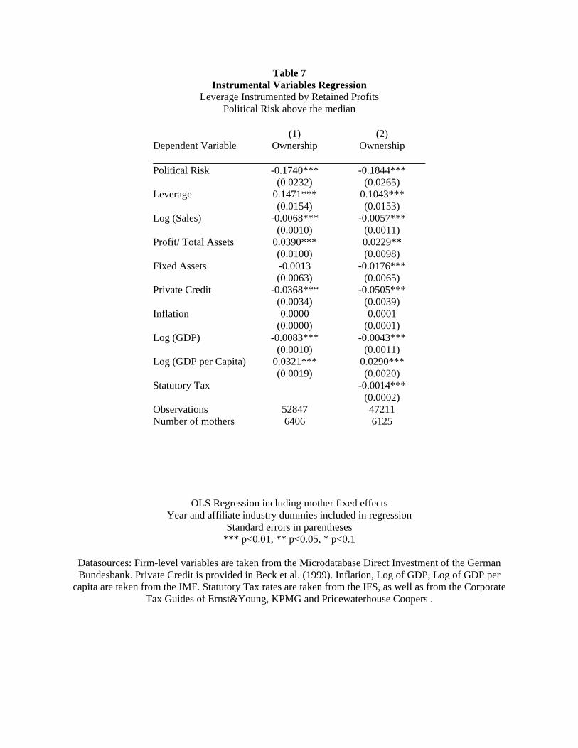
median, Table 6 and 7 for those enterprises facing a higher than average political risk.
When we compare the influence that political risk has on the capital structure in high
and low risk countries, our findings are the following: First, we find that the influence of
political risk on the level of leverage is more than twice as large when political risk is low
than when it is high. This is consistent with our Hypothesis 4 : In countries with less severe
political risk (Scenario 3), we expect the influence of political risk on the level of leverage
to be more positive than otherwise (Scenarios 1 and 2).
Second, we find that the influence of political risk on the ownership share is less sig-
nificant when political risk is is low as compared to when political risk is high. This is
consistent with our Hypothesis 2. The less severe is political risk (Scenario 3), the less
negative is its effect on the ownership share.
19
A second way to capture different types of political risk is by analyzing its interaction
with GDP per capita. In countries where GDP per capita is high we expect political risk
to act in its less severe form while in countries where GDP is low we expect that the
consequences of political risk on MNE are more severe.
In Table 8 and 9 we report the effects of political risk on leverage and ownership,
containing an interaction term between GDP per capita and political risk. While the effect
of both GDP per capita and statutory taxes on the level of leverage remain positive, there is
a drastic change in the coefficient of political risk in the leverage regression. This coefficient
is now negative and significant, while the coefficient of the interaction term between GDP
per capita and political risk is positive and significant.
Therefore, we find that the way MNE adapt their level of leverage in response to political
risk depends on GDP per capita. In countries where GDP per capita is low and we therefore
expect political risk to be severe, MNE lower their level of leverage in response to political
risk. In countries with higher GDP and less severe consequences of political risk, we find
that MNE finance their affiliates with a higher level of debt when political risk increases.
These findings again support our Hypothesis 4: the total effect of political risk is less likely
to be negative, the less severe the political risk scenario.
For the ownership share, we find that the coefficient of political risk remains negative
when the interaction term between political risk and GDP per capita is included. The
interaction term, however, has a positive and significant coefficient. Therefore, in countries
where GDP per capita is high, the influence of political risk on the ownership share is
less negative than when political risk is low. This supports our Hypothesis 2: The less
severe the political risk scenario, the less negative is the total effect on political risk. These
findings show that the the response of MNE to political risk is not at all homogenous, but
it strongly depends on the type of political risk present.
8 Conclusion
In this paper, we have investigated both theoretically and empirically how MNEs adapt
their capital structure choices in the presence of political risk. Not surprisingly, political
risk in general is bad for the profitability of a MNE as a whole. However, as our analysis has
shown, different types of political risk may have very different economic effects for different
20
stakeholders of the firm. Of course, equity holders as the residual claimants always suffer
from political risk and therefore want to reduce their exposure by limiting their ownership
share. Debt holders, in contrast, need not be affected in the same way. As a consequence,
the impact of political risk on debt financing may differ from that on equity financing.
This is why the effect of political risk on the optimal leverage turns out to be different for
different types of political risk.
Our analysis suggests that when it comes to assessing the potential effects of political
risk, it is important to distinguish different types of stakeholders and how they are affected
by different political measures. Only then is it possible to determine the optimal reaction
of the investor to this risky environment.
Another insight from our analysis is that the choices of ownership share and leverage are
interdependent and hence total effects of political risk may substantially differ from direct
effects. In particular, if leverage and ownership ratio are positively related, as observed,
then the total effects are smaller than direct effects. Thus, if one of the two choice variables
is not available, due to political restrictions on ownership shares or capital requirements, the
investor will react more strongly with the remaining choice variable. Suppose for example
that a government imposes a minimum capital rule to enforce more equity financing. Then
this will make the multinational investor limit his exposure by choosing an even smaller
ownership share. Governments need to be aware of this interaction when designing their
rules on multinational investments.
21
Mathematical Appendix
Solution of the base line model
The investor’s maximization problem is characterized by the following two first order con-
ditions.
dU
dα= (1− t)
[12R− (1− s)(1 + r) + 1
2− sD
]− (I −D)C ′ = 0 (34)
dU
dD= −α(1− t)
(2− s)
[(1− s)(1 + r) + 1 + (1− s)
dr
dDD
]+ αC ′ = 0 (35)
From the first order conditions we derive further
d2U
dα2= −(I −D)2C ′′ < 0 (36)
d2U
dαdD=
d2U
dDdα= − 1− t
2− s
[(1− s)(1 + r) + 1 + (1− s)
dr
dDD
]+ C ′
︸ ︷︷ ︸=0
+(I −D)αC ′′
= (I −D)αC ′′ > 0 (37)
d2U
dD2= −α2C ′′ − α(1− t)(1− s)
2− s
(2
dr
dD+
d2r
dD2D
)< 0 (38)
This gives us the following matrix
F =
∣∣∣∣∣∣∣−(I −D)2C ′′ (I −D)αC ′′
(I −D)αC ′′ −[α2C ′′ + α(1−t)(1−s)
2−s
(2 dr
dD + d2rdD2 D
)]
∣∣∣∣∣∣∣
It is straightforward to show that
|F | = (I −D)2C ′′α(1− t)(1− s)2− s
(2
dr
dD+
d2r
dD2D
)> 0 (39)
so that the first order conditions describe a maximum.
Proof of Result 1
The investor’s maximization problem is now characterized by the following two first order
conditions.
dU
dα= (1− t)(1− π1)
[12R− (1− s)(1 + r)
2− sD
]− 1− t
2− sD − (I −D)C ′ = 0 (40)
dU
dD= −α(1− t)(1− π1)(1− s)
(2− s)
[(1 + r) +
dr
dDD
]− α(1− t)
2− s+ αC ′ = 0 (41)
22
From the first order conditions we derive further
d2U
dα2= −(I −D)2C ′′ < 0 (42)
d2U
dαdD=
d2U
dDdα= −(1− t)(1− π1)(1− s)
2− s
[(1 + r) +
dr
dDD
]− 1− t
2− s+ C ′
︸ ︷︷ ︸=0
+(I −D)αC ′′
= (I −D)αC ′′ > 0 (43)
d2U
dD2= −α2C ′′ − α(1− t)(1− s)(1− π1)
2− s
(2
dr
dD+
d2r
dD2D
)− α(1− t)
2− s< 0(44)
This gives us the following matrix
F =
∣∣∣∣∣∣∣−(I −D)2C ′′ (I −D)αC ′′
(I −D)αC ′′ −[α2C ′′ + α(1−t)(1−s)(1−π1)
2−s
(2 dr
dD + d2rdD2 D
)+ α(1−t)
2−s
]
∣∣∣∣∣∣∣
It is straightforward to show that
|F | = (I −D)2C ′′α(1− t)2− s
[(1− π1)(1− s)
(2
dr
dD+
d2r
dD2D
)+ 1
]> 0 (45)
so that the first order conditions describe a maximum.
For our comparative statics analysis we need to determine
d2U
dαdπ1= −
[12R− 1− s
2− s(1 + r)D
]< 0 (46)
and
d2U
dDdπ1=
α(1− t)(1− s)2− s
[1 + r +
dr
dDD
]− α(1− t)(1− π1)(1− s)
2− s
[dr
dπ1+
d2r
dDdπ1D
]
(47)
Recall that r is implicitly determined by
(1− π1)(1 + r)− 2− s
21− π1
R(1 + r)2D − 1 = 0 (48)
Using the implicit function theorem we can derive from this
Schnitzer, M. (1999): “Expropriation and control rights: a dynamic model of foreign
direct investment,” International Journal of Industrial Organization, 17, 1113–37.
Stein, J. C. (1998): “An Adverse-Selection Model of Bank Asset and Liability Man-
agement with Implications for Transmission of Monetary Policy,” RAND Journal of
Economics, 29(3), 466–486.
(2003): “Agency, Information and Corporate Investment,” in Handbook of the
Economics of Finance, ed. by G. Constantinides, M. Harris, and R. Stulz. North Holland,
Amsterdam.
31
Thomas, J., and T. Worrall (1994): “Foreign direct investment and the risk of expro-
priation,” Review of Economic Studies, 61, 81–108.
32
Table 1 Descriptive Statistics
Definition Mean Std. deviation
Min* Max*
Dependent Variables Leverage Debt/ Total Capital 0.6112 0.3019 0.000 1.001Ownership Share Share of affiliate’s equity
held by German mother 0.7844 0.3447 0.000 1.000
Independent Variables (firm-level) Fixed/ Total Assets 0.2497 0.2695 0.0000 1.000Log( Sales) 9.1442 1.5031 6.9078 17.4813Profit/ Total Assets 0.0251 0.2379 -13.5080 27.4530Retained Profits/ Total Assets
0.0574 0.1393 0.0000 1.000
Independent Variables (country-level) Inflation 4.163699 15.1492 -29.2000 1061.2000Log(GDP) 6.1387 1.5981 -1.3174 9.3703Log(GDP per Capita) 9.6279 1.0499 4.4938 11.1656Political Risk Index between zero and one
with a higher index reflecting higher political risk.
0.1875 0.0880 0.0392 0.7474
Private Credit Ratio of private credit lent by deposit money banks to total GDP
0.8144 0.4090 0.0130 1.7850
Statutory Tax 33.7706 6.3533 10.0000 53.0000 *Averaged over three affiliates
Table 2 The Impact of Political Risk on Affiliate Leverage and Ownership Share
Year and affiliate industry dummies included in regression Standard errors in parentheses
*** p<0.01, ** p<0.05, * p<0.1
Datasources: Firm-level variables are taken from the Microdatabase Direct Investment of the German Bundesbank. Private Credit is provided in Beck et al. (1999). Inflation, Log of GDP, Log of GDP per
capita are taken from the IMF. Statutory Tax rates are taken from the IFS, as well as from the Corporate Tax Guides of Ernst&Young, KPMG and Pricewaterhouse Coopers .
OLS Regression including mother fixed effects Year and affiliate industry dummies included in regression
Standard errors in parentheses *** p<0.01, ** p<0.05, * p<0.1
Datasources: Firm-level variables are taken from the Microdatabase Direct Investment of the German Bundesbank. Private Credit is provided in Beck et al. (1999). Inflation, Log of GDP, Log of GDP per
capita are taken from the IMF. Statutory Tax rates are taken from the IFS, as well as from the Corporate Tax Guides of Ernst&Young, KPMG and Pricewaterhouse Coopers .
Table 4 The Impact of Political Risk on Affiliate Leverage and Ownership Share
Year and affiliate industry dummies included in regression Standard errors in parentheses
*** p<0.01, ** p<0.05, * p<0.1
Datasources: Firm-level variables are taken from the Microdatabase Direct Investment of the German Bundesbank. Private Credit is provided in Beck et al. (1999). Inflation, Log of GDP, Log of GDP per
capita are taken from the IMF. Statutory Tax rates are taken from the IFS, as well as from the Corporate Tax Guides of Ernst&Young, KPMG and Pricewaterhouse Coopers .
Table 5 Instrumental Variables Regression
Leverage Instrumented by Retained Profits Political Risk below the median
OLS Regression including mother fixed effects Year and affiliate industry dummies included in regression
Standard errors in parentheses *** p<0.01, ** p<0.05, * p<0.1
Datasources: Firm-level variables are taken from the Microdatabase Direct Investment of the German Bundesbank. Private Credit is provided in Beck et al. (1999). Inflation, Log of GDP, Log of GDP per
capita are taken from the IMF. Statutory Tax rates are taken from the IFS, as well as from the Corporate Tax Guides of Ernst&Young, KPMG and Pricewaterhouse Coopers .
Table 6 The Impact of Political Risk on Affiliate Leverage and Ownership Share
Year and affiliate industry dummies included in regression Standard errors in parentheses
*** p<0.01, ** p<0.05, * p<0.1
Datasources: Firm-level variables are taken from the Microdatabase Direct Investment of the German Bundesbank. Private Credit is provided in Beck et al. (1999). Inflation, Log of GDP, Log of GDP per
capita are taken from the IMF. Statutory Tax rates are taken from the IFS, as well as from the Corporate Tax Guides of Ernst&Young, KPMG and Pricewaterhouse Coopers .
Table 7 Instrumental Variables Regression
Leverage Instrumented by Retained Profits Political Risk above the median
OLS Regression including mother fixed effects Year and affiliate industry dummies included in regression
Standard errors in parentheses *** p<0.01, ** p<0.05, * p<0.1
Datasources: Firm-level variables are taken from the Microdatabase Direct Investment of the German Bundesbank. Private Credit is provided in Beck et al. (1999). Inflation, Log of GDP, Log of GDP per
capita are taken from the IMF. Statutory Tax rates are taken from the IFS, as well as from the Corporate Tax Guides of Ernst&Young, KPMG and Pricewaterhouse Coopers .
Table 8 The Impact of Political Risk on Affiliate Leverage and Ownership Share
Year and affiliate industry dummies included in regression Standard errors in parentheses
*** p<0.01, ** p<0.05, * p<0.1
Datasources: Firm-level variables are taken from the Microdatabase Direct Investment of the German Bundesbank. Private Credit is provided in Beck et al. (1999). Inflation, Log of GDP, Log of GDP per
capita are taken from the IMF. Statutory Tax rates are taken from the IFS, as well as from the Corporate Tax Guides of Ernst&Young, KPMG and Pricewaterhouse Coopers .
OLS Regression including mother fixed effects Year and affiliate industry dummies included in regression
Standard errors in parentheses *** p<0.01, ** p<0.05, * p<0.1
Datasources: Firm-level variables are taken from the Microdatabase Direct Investment of the German Bundesbank. Private Credit is provided in Beck et al. (1999). Inflation, Log of GDP, Log of GDP per
capita are taken from the IMF. Statutory Tax rates are taken from the IFS, as well as from the Corporate Tax Guides of Ernst&Young, KPMG and Pricewaterhouse Coopers .