Who should handle retail? Vertical contracts,

customer service, and social welfare in a Chinese

mobile phone market∗

Jia Li† Charles C. Moul‡

December 2014

Abstract

Using data on mobile phone handset sales from a single retail store, we examine

the impact of different retail responsibility designations and vertical contracts on seller

service provision, firm profitability, and social welfare. During our sample, this store

switched from retailer-managed retailing with linear pricing contracts to manufacturer-

managed retailing with revenue-sharing contracts. We estimate consumer demand and

manufacturer cost parameters. Demand estimates indicate a large positive shift that

coincided with the vertical change, consistent with improved retail customer service.

Welfare estimates suggest that consumers derived substantial surplus from the im-

proved customer service in addition to that from lowered prices.

Keywords: Marketing channel, vertical relationship, channel switch, revenue-sharing

contract, customer service, structural models, choice modeling, mobile phones

JEL codes: D43, L14, L63, L81, M31

Manufacturers selling directly to consumers in retail stores and compensating retailers

through revenue-sharing contracts has become common in the U.S.,1 and it is a long-standing

∗We thank James Reeder, Sangwoo Shin, Michael Walrath, participants at the 2010 International In-dustrial Organization Conference, several anonymous referees and the Editor for excellent comments and

suggestions. We are also grateful to Wenshu Zhang for excellent research assitance. Any remaining errors

are our own.†Purdue University Krannert School of Management, Department of Management (Marketing Area),

West Lafayette, IN 47907, USA. Tel: 765-496-1172. Email: jial@purdue.edu‡Corresponding author. Miami University Farmer School of Business, Department of Economics, Oxford,

OH 45056, USA. Tel: 513-529-2867. E-mail: moulcc@miamioh.edu1Louis Vuitton in Saks Fifth Avenue and Apple in Best Buy are two notable examples. In fact, the

cosmetics sections at almost all the major U.S. department stores (e.g., Bloomingdale’s, Macy’s, Neiman

Marcus, Nordstrom, and Saks Fifth Avenue) are managed under revenue-sharing contracts. The same

practice is also observed in the apparel category in the aforementioned stores (Jerath and Zhang, 2010).

1

practice in China and Japan.2 A similar arrangement is also popular in the online market

and the emerging mobile platform.3 In these scenarios, the manufacturer sets the retail price

of its product; retailer responsibilities, such as staffing and inventory management, are also

borne by the manufacturer. The manufacturer then pays the retailer a percentage of the total

sales revenue that it realizes in the store. The pricing implications of such revenue-sharing

contracts compared to traditional contracts in which retailers pay manufacturers per-unit

wholesale prices (linear pricing) have already received substantial theoretical and empirical

scrutiny.4 There has, however, been relatively little attention paid to the implications of

manufacturers shouldering traditional retailer responsibilities. This gap applies especially to

non-price margins of the retailer experience, broadly referred to in this study as customer

service.5

The impact of such a shift of retail responsibility and contractual type on service-quality

is ambiguous. A retailer performing the sales function might provide higher (e.g., more

objective) service than manufacturers could be expected to provide if they sold their products

to consumers themselves. Alternatively, the retailer might offer less in the way of service.

Tirole (1988, 177-8) shows that a monopolist retailer under linear pricing will provide less

than the industry profit-maximizing level of customer service; furthermore, a multiproduct

retailer knows that at least some lost sales of one brand arising from lower customer service

will be recaptured in sales of competing brands at the same store. Besides these incentive

issues, the relative cost advantage in the provision of service-quality may also be an important

determinant of customer service with respect to regime. In short, how consumer respond to

the retailing regime is an empirical question.

We address the question of how well manufacturers provide retail customer service by

examining a Chinese retailer’s policy shift in its contracts with all of its mobile phone handset

2A survey from 30 upscale department stores across major Chinese cities indicated that about 80 percent

of product categories were managed under this type of contract during our sample (Wu, 2005).3Amazon.com provides “marketplaces” where individual sellers can list their items and set prices. In

exchange for the hosting services, Amazon.com receives a percentage of the sales price (usually 10-15%) if

an item is sold. The online application stores (e.g., the Apple Store and Android Market) also adopt this

type of contract to sell applications from different developers. In Apple’s App Store, developers set the price

of the individual iOS app and share a percentage (usually 30%) of their revenues with Apple.4Dana and Spier (2001) and Cachon and Lariviere (2004) are prominent theory examples, and Mortimer

(2008) is a pioneering empirical example. Pricing has also been the primary focus in empirical work on

vertical relationships more generally. From industrial organization, see Villas-Boas (2007, 2009), Manuszak

(2010), Bonnet and Dubois (2010) and Ferrari and Verboven (2012), and from marketing see Chen, John,

and Narasimhan (2008), Kadiyala, Chintagunta, and Vilcassim (2000), Kim et al. (2001), and Sudhir (2001).5The literature on exclusive reselling and franchising (e.g., Desai and Srinivasan, 1995; Lafontaine and

Slade, 1997 and 2008) has long concerned itself with the provision of customer service, but this has not

generally spilled over into the context of retailers selling the goods of several distinct manufacturers.

2

manufacturers.6 Before the shift, the retailer and manufacturers engaged in retailer-managed

retailing with traditional linear pricing contracts. That is, the retailer was responsible for

retail prices and the staffing that handled all manufacturer brands. After the shift, the

retailer and manufacturers engaged in manufacturer-managed retailing with revenue-sharing

contracts. Under this regime, manufacturers operated their own booths and hired their own

sales staff to sell their products inside the store. This policy change thus facilitates a clean

before-and-after study of how consumers respond to changes in the retail-manager.

Figure 1 presents preliminary evidence that the retailing regime switch coincided with

an increase in quantities sold, an increase that we hypothesize stemmed from manufacturers

providing higher service quality. The figure shows brand-normalized weekly quantities for

the 70 weeks when our retailer’s phone-sales location was unchanged from when the regime

switch occurred (week 54).7 Estimates indicate an increase of one half of a brand standard

deviation ( = 049 5) in the last 17 weeks of the period (after the switch) compared

to the first 53 weeks. This happens despite the fact that phone sales at our retailer over

the entire sample tended to display no growth or a secular decline. This increase in sales,

of course, could stem from any number of sources besides our hypothesized higher service

quality, including but not limited to predictable seasonality, new and more preferred brand

characteristics, and lower prices that accompanied the regime switch.8 We therefore use data

surrounding this shift and vertical models appropriate to the regimes to structurally estimate

consumer demand and (inferred) marginal costs. After estimating the impact of any quality

changes that accompany the contractual switch, we then explore welfare considerations under

various counterfactual scenarios, enabling us to disentangle the various aspects of the vertical

contracts.

Available data are rarely ideal for structural applications, and our application is no dif-

ferent. In particular, our data come from a single retailer in the market. We lack information

on the number of retail competitors or the market structure, let alone competitors’ prices

and quantities. To address this concern, we assume an oligopoly of firms and estimate

6While phones and service plans in China were not bundled at the time of our sample, previous work

on mobile phones has focused on the U.S. model (in which phone bundling dominates) and thus taken the

service plan as the primary focus. See Xiao, Chan, and Narasimhan (2008), and Ascarza, Lambrecht, and

Vilcassim (2012).7Brand quantities differ sufficiently in their means and variances that standardizing by each is necessary

for a visual representation. Over this subsample, the plotted value for brand at week is =−√(−)2

.

8The impact of the regime change on pricing depends on the original wholesale price and the new rev-

enue shares and is thus also ambiguous. Liu and Shuai (forthcoming) thoroughly explore how demand

fundamentals and relative competitiveness determine the equilibrium impacts of such contractual shifts.

3

demand first in isolation and then jointly with cost, both conditional on the specific -firm

oligopoly assumption. As Moul (2012) points out, if the assumption on the value of is

innocuous, demand parameters should be similar across the isolated and joint estimations.

A significant divergence of demand-alone and joint estimates of demand then indicates a

contradiction of the maintained assumption on market structure. We are thus able to draw

some limited conclusions on market structure even in the absence of manufacturer cost data.

While we assume that these hypothetical firms are largely similar (essentially symmetric)

to our observed retailer, our model allows for our retailer to face idiosyncratic changes to

demand (e.g., relocating phone sales area within store). In such cases, we use our model and

its profit-maximizing conditions to construct the equilibrium prices that would have been

charged by other retailers.

Our estimates for demand and cost are plausible and consistent with our retailer facing

a reasonable degree of retail competition (at least three firms). Consumers respond to

touch screens, the presence of a second screen, the main display being in color, the quality of

playback, game capabilities, and camera capabilities.9 These characteristics are all associated

with higher costs of production. We also find that demand increased substantially when

retail responsibility was shifted from our retailer to manufacturers. This suggests that the

vertical contracts could have substantial impacts on not only the equilibrium retailer and

manufacturer prices, but also (through changed incentives for and differing costs of service

provision) demand itself. The solutions of various counterfactual scenarios indicate that

both consumer surplus and welfare increased by about 15% when the sector moved from

the original regime to the new regime. Furthermore, most of the additional market-wide

consumer surplus that was generated came from this improved customer service rather than

the lower prices that we observed. The retailer and manufacturer profits implied under

these counterfactuals suggest that, consistent with observations from the industry in China,

manufacturers have a sizable cost advantage in retail quality provision from training staff

and inventory management.

The paper is structured as follows. First, we describe our data and the circumstances

of the regime switch that shifted retail responsibilities from our retailer to manufacturers.

The second section presents a model of demand and price competition for manufacturers

and retailers in the Chinese mobile phone industry. We discuss details regarding the model

estimation in the third section. The fourth and fifth sections present estimates and counter-

9As Apple did not introduce the iPhone until June 2007, our sample (2003-2006) predates the smartphone

era, but our estimates foreshadow the product characteristics that the industry later emphasized.

4

factuals, while the final section concludes with suggestions for future research.

1 Phone Data in our Chinese Market

Our data come from a department store located in a Chinese city with five to ten million

residents. Like most other department stores in China but unlike most U.S. stores, the

store operated at a single very large location during the sample period (2003-2006). The

store is among the largest of its kind across China, selling products in many categories (e.g.,

apparel, apparel accessories, cosmetics, jewelry, watches, home furnishings, bed and bath

products, appliances, electronics, toys, food). There was only one other department store of

comparable size and product selection in our retailer’s city, but there were also many smaller

department stores and consumer electronics specialty stores and (later in the sample) mobile

phone specialty stores.

Within the store, the various categories and products are managed under two verti-

cal agreements between manufacturers and the retailer. As of 2011, about ten percent of

all products were managed by the traditional agreement of retailer-managed retailing with

linear pricing contracts. The majority of products, however, were managed by manufacturer-

managed retailing with revenue-sharing contracts. These products are sold in dedicated areas

in which display areas are placed. During the sample period, the mobile phone handset de-

partment occupied about 18,000 ft2 (one-third the area of an American football field). While

this area of the store was sometimes spaced with aisles to permit consumers to walk freely

within it, booths could also be placed immediately adjacent to each other with sales staff

away to the side until they were needed. Throughout our sample, sales staff received a base

salary and commissions on sales, with over 50% of ex post pay deriving from commissions.

While we do not have data on average commission per phone sold, information on typical

sales-staff incomes and work-weeks suggests that these per-phone commissions were small

relative to the retail prices of phones (about 1%).

We observe weekly transaction-level sales data of mobile phones including unit sales and

average retail price at the model level from January 2003 to December 2006 (208 weeks).

During this time frame, department stores such as our retailer were the primary place from

which Chinese shoppers bought their mobile phones. This mobile phone category saw a

store-driven shift from linear pricing to revenue sharing in early 2006. The store decided in

late February of 2006 to change its agreements with all brands in the category so that the

retail responsibilities were shifted to the individual manufacturers in the middle of April.

5

This decision was prompted by the discovery that our retailer’s foremost competitor had

recently decided to make the same switch, though it had not yet done so.10 Our model

therefore assumes that the vertical agreement change was not due to any external demand

shocks or the actions of the manufacturers. We further assume that all other retailers in

the market also switched to this type of vertical contract at the same time. While this is an

extreme assumption, store managers indicate that all relevant competing retailers did make

the contractual switch within a two-month window.

It is obvious that the regime switch might have prompted a change in pricing, but there

are also a few mechanisms by which customer service and inventory management may have

improved. Conversations with management indicated that total staffing did not appreciably

change with the regime switch, and contractual terms with sales staff were also invariant

to the regime. The most straightforward candidate mechanisms are therefore eliminated.

Economies of scale in training is perhaps the most direct remaining avenue. Each manu-

facturer has the opportunity to assemble and train the sales staff from all the retailers in a

(rather large) geographic area at the same time. A retailer, though, has only its own staff

against which to amortize the fixed cost of quality-training. The retailer also has no obvious

special knowledge regarding the brands and newly introduced models, a defect not shared

by the manufacturer. Last, manufacturer-managed retail makes it possible for the manufac-

turer to pool inventory at the city-level rather than at the retailer level as would be necessary

under retailer-managed retail. Stockouts and disappointed customers may therefore be less

likely occurrences.

The number of brands sold in the store during the entire sample period varied from 56

to 65; however, only 12 brands had a consistent presence in the store for the entire four year

period. These brands were the expected global leaders (e.g., Nokia, Samsung, Motorola)

accompanied by a few Chinese brands (e.g., Bird, Konko). A number of other brands were

only available in the store for one or two years before manufacturers decided to exit the

market or before the store replaced them with new brands. There were also mergers among

manufacturers. Asus, which had previously had minimal market presence, purchased the

Chinese rights to Siemens in 2005 and so is referenced throughout as Siemens/Asus.

10During our discussions with store managers, they stressed that this management change occurred quickly

and smoothly and confirmed that no major exogenous events such as changes in production and selling costs

or significant entry and exit in the industry had contributed to their decision. They viewed the management

change as consistent with the store policy and retailing trends in China. We heard no stories regarding how

the technological progress that prompted this switch might have affected the underlying sales technology or

market structure.

6

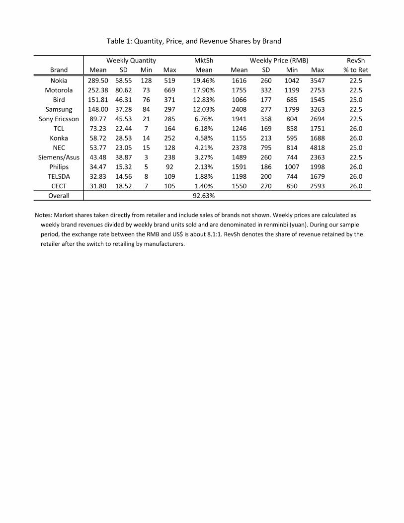
We consider the 12 brands that had a consistent presence in our sample. Table 1 provides

summary statistics for the brands’ weekly quantities sold, average retail prices of the brands,

and shares of revenue paid by manufacturer to retailer after the contract switch. Overall,

the 12 brands dominated category sales throughout the four years of the sample with an

average cumulative market share of about 93%. While five brands discontinued sales at the

retailer when the regime switch occurred, they were all quite small with cumulative market

share of 2.4%. This absence is therefore unlikely to be able to generate the demand increase

that we observe for the remaining brands. We also compared the pricing and sales trends

for the twelve brands with the overall category and did not find any significant difference.

Despite the fact that sales of these brands will be mistakenly aggregated with the choice of

consumers to buy no phone, we therefore believe that the exclusion of other brands should

not have a major impact on the empirical results.

The observed revenue shares that the retailer contracted with the manufacturers are con-

stant in our sample after they were introduced. Conversations with store managers indicate

that revenue shares were chosen in large part so that the new equilibrium prices would not

be too different from the old. Revenue shares do exhibit some slight cross-manufacturer

variation, as three manufacturers paid 22.5% of revenues, two paid 25%, and five paid 26%.

It appears that brands with higher sales were generally given more favorable (lower) revenue

shares than weaker brands. The broad similarity of the revenue shares’ levels somewhat miti-

gates the concern that endogenously determined revenue shares might corrupt our estimation

strategy.

Our empirical analysis employs brand-level weekly sales and average transaction prices,

both of which are constructed by aggregating the transaction-level (model-level) sales data

provided by the store.11 We used public websites to supplement the sales data with the

characteristics for each model sold in the store during the sample period.12 The collected

characteristics are fairly exhaustive, including form factor (shape of phone, e.g., flip), cellu-

lar radio frequencies, battery life (as measured in talk-time and standby-time), number of

available colors, size of internal memory, and video camera capabilities.13

We aggregate these model-level characteristics up to the brand-level to match our brand-

level sales and price data, weighting characteristics by a model’s units sold as a share of the

11This aggregation to the brand-level is necessary because many models of smaller brands earn no sales in

many weeks, even though they were presumably still available.12We specifically used http://www.3533.com/phone/ (in Chinese) and http://www.gsmarena.com/ (in

English).13A complete list of the product characteristics that we considered is available in Table A1 of the appendix.

7

brand’s total units sold. Unlike the brand fixed effects that we also include, these brand-level

characteristics vary over the sample, and we use them as regressors and then again when

constructing instruments. We also include variables that capture the breadth of a brand’s

portfolio, specifically the number of different models that a brand sold in a week and a

Herfindahl index of the concentration of those sales within particular models. Descriptive

statistics of brand-level characteristics are provided in Table 2.

There are three plausibly exogenous events that occur over the sample’s four years. In

addition to the critical policy switch from linear pricing to revenue sharing (Switch) in

April 2006 (Week 175 of our 208 week sample), there were two selling-area relocations.

The first relocation of the phone area to a more highly trafficked region of the store (1 st

Relocation) occurred in early May 2005 (Week 122). The other relocation of the phone area

(2 nd Relocation) occurred at the beginning of September 2006 (Week 192), leaving 17 weeks

of the sample for us to observe manufacturers selling in the new location. Discussions with

the retailer suggested that this second relocation was to an inferior location compared to the

first relocation.14

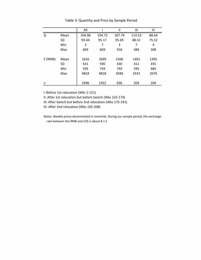
Table 3 displays summary statistics of quantities and retail prices at the brand level

for the sample and then across the four potentially distinct regimes: before 1 st Relocation,

after 1 st Relocation but before Switch, after Switch but before 2nd Relocation, and after 2 nd

Relocation. Over the entire sample, the average brand weekly units sold is about 105, but,

as evidenced by the standard deviation and range, there is substantial variability around

that mean. Final prices paid by consumers over the entire sample averaged U1616 or aboutUS$ 200 at the period’s exchange rate of $1 to U8.1.15 Average prices decline across all foursubsamples, and the average quantities are consistent with the relocations having impacts

as described by our retailer’s managers. The magnitude is not large, but the uptick in sales

following the switch to manufacturer-managed retailing is also apparent.

Descriptive estimation can shed light on the raw variation in the data, and Table 4

displays such estimates for quantity and price.16 All regressions include a second-order

polynomial of a time trend as well as 11 month and 12 brand dummies (not shown). Several

broad results are apparent. The estimated impacts of product characteristics on quantity

14According to store management, the first relocation occurred because the store decided to renovate the

floor where the mobile phone area was located; the second occurred because the store used its previous

location to build a new facility.15We reference the Chinese currency interchangeably as the yuan (U) and the renminbi (RMB).16The F-stats at the bottom of Table 4 test the null hypotheses that our instruments have no explanatory

power beyond the listed regressors. We consider them in greater length when we introduce our identification

strategy and exclusion restrictions.

8

sold tend to be superficially counterintuitive, specifically negative for favorable features.

This presumably stems from the fact that brands with such features also have higher prices

and consequently lower sales. The opposite relationship (that is, the intuitive one) holds

between these features and price. The significant positive estimated impact of mass on price

presumably stems from mass proxying for unobserved features of phones that consumers find

desirable, and we will interpret mass in this light for the rest of our analysis.

Both relocation indicators are highly significant in the quantity regression, with the first

relocation boosting sales and the second negating that increase. The first relocation is also

estimated to have had a significant increase on brand phone prices. While our paper’s

emphasis is the importance of vertical contractual switches, the estimated magnitudes on

quantity are a pointed reminder that product placement warrants coequal treatment.

Most importantly for our purposes, we see that quantities increased substantially with

the channel switch. Brands are estimated to have sold an additional 25 phones compared to

their weekly average sales of 108. Prices, however, did not fall by much beyond that captured

by the time trend; the estimated coefficient on the indicator, while negative, is small

(1% of mean price) and not statistically different from zero. This is preliminary evidence in

favor of our paper’s key result that increased consumer demand came at least in part from

higher customer service and not simply lower prices.

2 Model of Consumers, Retailers, and Manufacturers

In line with the above description, we consider a situation in which data are available from

one retailer ( = 1) for = 1 brands (in which a brand corresponds to a manufacturer)

over = 1 periods in a single market with potential consumers.17 While we observe

only our retailer, we assume that the market contains essentially symmetric retailers, each

of which sells the same set of brands as our observed retailer. For each brand, the data contain

the average retail transaction price , the quantity sold , brand characteristics that may

affect demand and costs ( and respectively), and retailer characteristics .18 We also

17We observe the city’s population in 2000 from the 5th China Census and linearly interpolate from the

estimated population in 2008. Given our weekly observations, we divide this population measure by 52

for our market size in an attempt to capture the durability of mobile phones. While the assumption

is arbitrary, our key result (demand increase coinciding with switch to manufacturer-managed retailing) is

robust across a wide array of population assumptions.18Our model is similar to Villas-Boas and Zhao (2005) in that both model a market taking into account

all parties involved: the manufacturer, the retailer, and the consumer. Both models are then estimated

using data from only one retailer in the market. Villas-Boas and Zhao, though, have micro-level household

purchase data and do not consider competition among retailers in the market. Another difference is that

9

observe the proportion of revenue retained by the retailer () after the regime-switch.

2.1 A model of demand for mobile phones

Unlike the U.S. market, the Chinese mobile phone market did not bundle phones and service

plans during our sample period. We therefore follow Berry (1994) and assume that each

consumer makes a relatively straightforward discrete choice among possible phone brands

and retailers, reflecting preferences over characteristics including price and features such

as ringtone, game, and camera capabilities. Formally (and suppressing time subscripts for

notational convenience), consumer has conditional indirect utility for brand from retailer

given by

= − + + (1)

From (1), is the mean utility from observable characteristics of brand at retailer

, − is the mean disutility associated with the price of brand at retailer , and

represents the mean valuation of characteristics that all agents in the market observe but the

econometrician does not. We test the demand-shifting effect of the regime switch by including

a binary indicator for whether the week falls before or after the move to manufacturer-

managed retailing under revenue sharing.19

Consumers also have a no-purchase option, and this outside option is denoted = 0.

The weekly probability of a consumer choosing each retailer-brand option is therefore em-

pirically constructed as =. This now-common framework is explained in detail in

the appendix. We accommodate potential seasonality by following Einav (2007), specifying

0 = + 0 which motivates our inclusion of month fixed effects. Regarding the dis-

tributional assumption of , we follow McFadden (1978) by using the generalized extreme

value (GEV) model that generates a nested logit allowing for consumers to be more likely

to substitute among brands than to the option of no-purchase. This form of segmentation

mitigates mismeasurement of market size and has been useful in prior research (Berry and

Waldfogel, 1999; Einav, 2007). It is operationalized by including information on a choice’s

market share as traditionally defined (e = ).20

product differentiation is arguably more important in the mobile phone category than in their category

(ketchup).19Our eventual estimate therefore reflects the average impact across brands and ignores the small differences

in the retained revenue shares.20Nests within the inside options (e.g., non-Chinese brands vs Chinese brands) are alternative specifications

and remain for future research.

10

Let a brand’s market share be defined as that brand’s units sold as a share of all units sold,

denoted e = =1

=1

. The nested logit model then has the convenient transformation

ln() − ln(0) = + ln(e), with lying on the unit interval and capturing the im-

portance of inside-outside segmentation.21 This simple (but adequate) demand specification

is driven by both the single-retailer limitation and the necessary brand-level aggregation.22

Given its direct implications, we are able to focus our attention on the more interesting

supply-side.

The essential symmetry assumption

As discussed above, we have data on only the one retailer, and so we do not observe

the total market quantity sold. We accommodate this limitation in our data by assuming

an essentially symmetric -firm oligopoly in which our retailer is a participant. By sym-

metric, we mean that there are − 1 other retailers (identical to each other and denotedas = 2, with the observed retailer denoted as = 1) that sell the same brands as our

retailer and share a common valuation of unobserved characteristics (i.e., = ∀ ).Our assumption of symmetry, though, is essential rather than total in that our model can

accommodate observed idiosyncratic shocks incurred only by the observed retailer. Specifi-

cally and as discussed above, our retailer twice relocated the selling areas for mobile phones

during the sample period. A total symmetry assumption would imply that other retailers

would experience the same shock from this counter relocation. Our essential symmetry as-

sumption, on the other hand, allows this observed shock to be idiosyncratic, and thus the

observed retailer and these other retailers may charge different prices in equilibrium. Under

this -firm oligopoly assumption and letting 1 be the vector of demand parameters, we

denote the purchase probability as ( ; 1).

Allowing for more than one retailer has two immediate demand-side implications on

which we expand to link more closely to the extant literature. First, it will affect the

observed likelihood of consumers choosing the outside option of no purchase. As the observed

total purchase probabilities at retailer areP

=1 , the market-wide probability of no

purchase will be 0 = 1−P

=1 1 − ( − 1)P

=1 2. When assuming a fixed population

of consumers, larger values of will then cause the implied number of consumers making no

21The robustness of our results to choice of market size M stems from this allowance of inside-outside

segmentation and the estimation of the parameter. The only change of note under different assumed

populations is the number of retailers () that is needed to maintain the result that isolated-demand

estimates are close to joint-demand estimates.22Recent work on upstream contracts (e.g., Chen, forthcoming; Conlon and Mortimer, 2014; Ho, Ho, and

Mortimer, 2012) has primarily employed similar nested logit models of demand.

11

purchase to decrease. Second, it will lower any retailer-brand’s true market share for a given

brand, as the retailer-brand-specific market share to be included in the demand regression

must now be constructed as

e1 = 1P

=1 1 + ( − 1)P

=1 2(2)

to reflect the retailer-brand’s share of the entire market.

We then take to the data the demand equation

ln (1)− ln (0) = 1 − 1 + ln (e1) + 1 (3)

in which 0 and e1 are both dependent upon the assumed number of retailers . In thecase of total symmetry in which our retailer incurs no idiosyncratic shocks and all retailers

are identical in equilibrium, the above becomes

ln (1)− lnÃ1−

X=1

1

!= 1 − 1 + ln

Ã1

P

=1 1

!+ 1 (4)

As we will assume that the -firm oligopoly is constant across the sample, the appearance

of on the right-hand side will be absorbed into the intercept. There is some superficial

identification of on the left-hand side, but we expect to find that is not empirically iden-

tified by demand estimation. As will also appear in firms’ profit-maximization conditions,

though, identification may come from the supply side. It is this supply-side identification

suggested by Moul (2012) that we hope to exploit in comparing demand-only estimates and

demand-joint-with-cost estimates in order to pin down plausible market structures. We will

further discuss this inference of market structure in the estimation results section.

2.2 The pricing problems of phone manufacturers and retailers

We next turn to the supply side of the model. As we have discussed, mobile phones in our

data were sold first under the linear-pricing contract and then under the revenue-sharing con-

tract. The retail price is set by the retailer and individual phone manufacturers respectively

under the two contract formats. Consequently, we must construct the pricing problems of

manufacturers and retailers separately for the two regimes. For notational convenience in

the supply model, it is useful to note consumer behavior with quantities demanded rather

than with purchase probabilities . The demand function for brand at retailer is then

= · ( ; 1) = ( ; 1) (5)

12

The pricing problem under linear pricing

Under linear pricing, manufacturers first simultaneously choose their wholesale prices.

Next, multibrand retailers simultaneously choose retail prices for their brands given the

wholesale prices and other costs. In this stage, retailers act independently of one another

even though they have the same upstream manufacturers. To analyze the subgame perfect

Nash equilibrium (SPNE) of this model, we begin with the retail market and then examine

the equilibrium among manufacturers.

In the downstream sector, retailer sets prices for all its brands to maximize

Π =

X=1

¡ · ( ; 1)−

( ( ; 1))¢−

(6)

in which superscript denotes retailer terms, () is retailer ’s variable cost of providing

units of brand , and are retailer ’s fixed costs. We assume that variable costs are

() =

¡ +

¢ (7)

so that retailer ’s marginal cost of brand is constant and can be decomposed into a

wholesale price () and other brand-specific retailing costs (). In what follows,

reflects variable costs set by the manufacturer of brand , while involves other variable

costs not determined by the manufacturer. Note that we must assume that manufacturers

charge a wholesale price that is common to all retailers in our market in order to recover the

equilibrium prices of the unobserved other retailers.23

Assuming the existence of a pure-strategy Nash equilibrium in prices, retail prices for

retailer must satisfy the first order conditions

( ; 1) +

X=1

¡ − −

¢ ( ; 1)

= 0 (8)

for = 1 and = 1 . In matrix notation, retailer ’s system of first order

conditions can be expressed as

( ; 1) +∆1 ( ; 1) ·¡ − −

¢= 0 (9)

in which , , , and ( ; 1) are × 1 vectors of retail prices, wholesale prices,

retailing marginal costs, and quantities. The () element of the × matrix ∆1 is

23While this assumption is impossible to verify with data from only one retailer, our retailer’s managers

believed that it was largely correct.

13

( ;1)

. Solving for and stacking these equations yields a system of pricing equations

characterizing the decisions of all price-setting retailers:

=f + − e∆1 ( ; 1)−1 · ( ; 1) (10)

in which the × 1 vector f denotes stacked wholesale prices and the × matrixe∆−11 denotes vertically stacked inverses of the above × matrices ∆−11 .

This expression relates observed retail prices to wholesale prices, retail costs, and markups

reflecting market power at the retail level. A standard model of retail competition (e.g.,

Berry, Levinsohn and Pakes, 1995) would end at this point with a specification for costs as

a function of observed characteristics and an unobservable component as described in Berry

(1994). This system of retail pricing equations could then be estimated jointly with the

demand model.

Our model, on the other hand, has the additional layer of manufacturers. As in any

SPNE model, we work backwards. Downstream competition implies equilibrium prices ∗ =

¡ ; 1

¢that depend on all wholesale prices and retail costs as well as all demand

variables. Thus, the manufacturer of brand faces derived demand

X=1

e ¡ ; 1¢=

X=1

¡¡ ; 1

¢ ; 1

¢(11)

in which ¡ ; 1

¢is the vector of retail equilibrium price functions. Letting

superscript denote manufacturer terms, the manufacturer of brand chooses its wholesale

price for all retailers in order to maximize

Π =

¡ −

¢Ã X=1

e ¡ ; 1¢!−

(12)

in which is the manufacturer’s constant marginal cost of brand and is manu-

facturer fixed costs. Following our essential (rather than total) symmetry assumption on

retailers and suppressing the arguments of the derived demand functions, this becomes

Π =

¡ −

¢(e1 + ( − 1) e2)−

(13)

When setting the wholesale price, manufacturers account for the impact of cost changes

on the retail equilibrium as required in a SPNE. Notationally suppressing the dependence

of derived demand on all variables except and assuming the existence of a pure strategy

Nash equilibrium, the wholesale price that manufacturer charges to all retailers must satisfy

e1 ( ) + ( − 1) e2 ( )+14

¡ −

¢Ã X=1

X=1

1 ( )

( )

( )

+ ( − 1)X=1

X=1

2 ( )

( )

( )

!= 0 (14)

in which the cumulative response of brand ’s quantity to a change in its wholesale price ac-

counts for the impact of changes on on all retail prices of all brands and for the associated

effect of those price changes on the quantity demanded of brand . The retail equilibrium

price responses,( )

, can be derived from the retail profit-maximizing equations in (8)

via Cramer’s Rule. Given our relatively sparse demand specification, analytical expressions

for these retail price responses have closed form solutions. Implementation details are given

in the appendix.

As in the case of the retail sector, these first order conditions can be expressed in matrix

notation as e1 ( ) + ( − 1) e2 ( ) +∆2

¡ −

¢= 0 (15)

in which , , and are ×1 vectors. The × matrix ∆2 is diagonal with element

1

+( − 1) 2, in which derivatives reflect cumulative equilibrium responses to a change

in the wholesale price. Rearranging terms yields a vector of wholesale pricing equations

= − (∆2 ( ))−1(e1 ( ) + ( − 1) e2 ( )) (16)

This expression relates (unobserved) wholesale prices and manufacturer costs to manufac-

turer markups.

The crucial components of the model that apply before the policy shift (i.e., the linear

pricing regime) are the retail and manufacturer pricing equations. The retail pricing equa-

tions are similar to those in other empirical studies of oligopolistic industries. The difference

is the interpretation of part of the marginal cost as the wholesale price. The manufacturer

model then provides a characterization of the wholesale prices. Letting ∆−111 now denote the

× submatrix that is specific to our retailer, these two sets of pricing equations can be

combined to yield (for our observed retailer)

1 = 1 + 1 −∆−111 1 −∆−12 (1 + ( − 1) 2) (17)

relating observed retail prices to costs and markups from both the manufacturing and retail

sectors. Assuming that the total marginal cost of brand can be expressed as a linear function

of observable cost characteristics , unknown cost parameters 2, and an unobserved cost

component so that

+ = 2 + (18)

15

the combined pricing equations can be rewritten as the × 1 vector

1 = 2 −∆−111 1 −∆−12 (1 + ( − 1) 2) + (19)

In general, we cannot separately identify retail and manufacturer marginal costs without

observing wholesale prices. If, however, we are willing to assume that retailers incur zero

marginal costs aside from wholesale prices ( = 0 ∀ so = ), then manufacturer

marginal costs are identified. We will follow Villas-Boas (2009) and take this approach. In

this setting, staffing costs, which are presumably increasing with both size of sales staff and

customer-service quality, are then treated as a fixed rather than variable cost. As such, they

cannot be inferred from pricing decisions, but they will affect inferences on profit, as we will

discuss later in our counterfactuals.

Treating staffing costs as fixed rather than variable is an onerous assumption, but perhaps

less so given the relative magnitude of commissions per phone to the retail price (about

1%) and that sales staff did not appreciably change with the regime switch. This concern is

further undercut by the fact that, conditioning on the size of sales staff, the costs of increasing

customer-service quality will presumably be incurred in training rather than depending on

quantity sold. If, however, retailing generates strictly positive marginal costs, our inferred

wholesale prices and marginal costs for manufacturers will be overstated. When demand

and cost are jointly estimated, this assumption can also be expected to make demand less

elastic in order to fit the observed price and quantity. This would bias downward and

upward and most likely inflate estimates of both demand and cost.

The pricing problem under revenue sharing

After the policy switch to manufacturer-managed retailing and revenue sharing in our

data, manufacturers pay a fixed proportion of revenue to retailers. We observe this proportion

for our retailer and assume that it applies to the other hypothetical retailers as well. We must

assume either that a manufacturer jointly manages its booths at all retailers or that each

manufacturer’s booth at each retailer is managed independently. As our empirical results

are robust to either choice, we employ the simpler independent-booths assumption.

Using the above notation and letting denote the revenue share that the manufacturer

of brand allows the retailer to retain, each manufacturer chooses a retail price for each

retailer to maximize

Π =

¡(1− ) −

¢ ( ; 1)−

(20)

16

The corresponding first order condition resembles the earlier retailer first order condition,

with the exception of the leading revenue-share term:

(1− ) ( ; 1) +

µ¡(1− ) −

¢

¶= 0

In vector notation for each manufacturer,

(1− ) ( ; 1) +∆3 ( ; 1)¡(1− ) −

¢= 0 (21)

in which and are × 1 vectors. The × matrix ∆3 then has the ( ) element

( ;1)

. The pricing equations under revenue sharing for the manufacturer of brand

are

=1−

−∆−13 ( ; 1) · ( ; 1) (22)

and are empirically implemented by substituting = 2 + for the manufacturer’s

marginal cost. We then employ the pricing equation appropriate for our observed retailer.

This statement of the manufacturer’s pricing problem again assumes that a firm incurs no

marginal costs from retailing. Within this context, one might also consider a less restrictive,

but still not completely benign, assumption that manufacturers and retailers face the same

marginal cost of retailing. To the extent that retailing marginal costs are strictly positive

but the same between retailers and manufacturers, problems with inferences will be limited

to how industry profits are distributed between retailers and manufacturers.

The above model makes strong assumptions on consumer and firm behavior, but the

payoffs are substantial. The solved model enables us to map observed prices and quantities

to unobserved wholesale prices and manufacturer marginal costs under linear pricing and

manufacturer marginal costs under revenue sharing. With those variables in hand, we can

then make inferences on not only the level of industry profits but also the distribution of

those profits between retailers and manufacturers. These distributional consequences are

likely to be decisive when considering what changes in vertical contractual terms will be

mutually acceptable to all parties.

3 Model Estimation

3.1 Estimation methodology and Identification

Following the suggestion of Berry (1994) and Berry, Levinsohn, and Pakes (1995), the previ-

ously presented model of price competition and costs can be estimated through Generalized

17

Method of Moments (GMM) either jointly with the demand model or separately after de-

mand estimates are obtained. Either approach requires some set of instruments that are

correlated with prices and quantities but uncorrelated with the demand unobservables ;

joint estimation also requires instruments that are uncorrelated with cost unobservables .

In particular, we must construct the set of instruments that have the property that

[1] = [2] = 0 (23)

in which 1 are instruments for the demand side of the model and 2 are instruments for the

pricing equations. Consider the broader case of joint estimation. Letting () and ()

denote the demand and cost unobservables implied by a value of = {1 2}, the GMMestimator is defined as

= argmin

()0−1 0 () (24)

in which is an appropriately constructed matrix of instruments, is a positive definite

weighting matrix, and () = [ ()0 ()

0]0 with () = [1 () ()] and () =

[1 () ()].

Like much of the preceding literature on differentiated products going back to Berry

(1994), our identifying assumption for demand and cost is that product characteristics are

exogenously determined. This implies that product characteristics are orthogonal to demand

and cost unobservables and permits the use of a good’s non-price product characteristics as

regressors without the need for instruments. When combined with the exclusion restric-

tion that consumer utility for a good does not depend on other goods’ characteristics, the

assumption also permits the use of other goods’ product characteristics as instruments for

the initial good’s price and conditional market share. A brand’s competitive environment

therefore can in principle trace out both the demand curve and the cost curve (through the

pricing equation implied by profit-maximization).

This identification strategy is not without defects given the circumstances of our appli-

cation. There are three potential criticisms of this strategy: 1) endogenous product char-

acteristics in a fast-changing industry, 2) the use of endogenous market shares within the

construction of brand-level instruments, and 3) the explicit omission of an endogenous vari-

able (customer service quality). We discuss each of these three issues, noting that our

inclusion of brand fixed effects as both demand and cost regressors mitigates these concerns,

especially regarding the possibility of endogenous product characteristics.24

24The inclusion of brand fixed effects implies that [ ] contain only the deviations of product quality and

cost from the brand mean.

18

First, assuming exogenous product characteristics in an industry for four years seems

at odds with the observed levels of innovation and product introduction in mobile phones.

This aspect of our identification strategy would be violated, for example, if a manufacturer

faced a rival selling models that were highly desirable in inimitable ways that our variables

could not capture and then the manufacturer responded by introducing new models with

superior characteristics that we do observe (e.g., battery life or camera capabilities). An-

other restatement of our identification strategy is therefore that manufacturers introduce

new features in their models when exogenously determined technology permits. While new

product introduction is common in the mobile phone industry, the substantial length of time

to move from concept to product suggests that this assumption may be relatively benign.

Second, we aggregate model-level characteristics up to brand-level characteristics using

each model’s share of brand sales. The use of endogenously determined model sales within

instruments may raise some concern. So long as one brand’s mean valuation of unobserved

characteristics () is uncorrelated to how another brand’s total sales are divided among its

several models, the moment condition will still be valid.

Third, the explicit omission of an endogenous variable (the quality of customer service)

complicates the above discussion somewhat. In such a situation, the above demand distur-

bance is the sum of an exogenous component and the utility impact of the unobserved

but endogenous customer service. This latter component may be systematically correlated

with both exogenous regressors and instruments. Assume that mean utility is increasing

in customer service and that the relevant section of demand is convex (2

2 0), as occurs

in the GEV family when purchase probabilities are relatively small. The retailer’s profit-

maximizing customer service level for a brand then increases with that brand’s favorable

characteristics and decreases with other brands’ favorable characteristics. Such a violation

of the exclusion restrictions would bias regressor coefficients away from zero (up for favor-

able characteristics), essentially attributing the attendant customer service entirely to the

exogenous variable. This concern will be mitigated somewhat under the original regime by

the retailer recognizing portfolio effects when choosing customer service levels as well as by

the fact that the retailer carries all models and brands.

Should our identification strategy be violated in any of these three ways, these biases will

generate overstatements of inside-outside segmentation and understatements of consumer

responsiveness to price. Each of these would in turn imply overstated estimates of the

impact on demand of switching between vertical regimes.

19

For the demand-side instruments, we include own-brand characteristics, , excluding

price and ln (e). We additionally employ instruments related to competing products in themarket. These variables include the total number of models offered by competitors as well

as the summed brand characteristics of competitors (e.g., summed percentage of sold phones

with a second screen). We have 56 exogenous demand regressors: 3 regime indicators (Switch,

1 Relocation, 2 Relocation), 28 product characteristics, 2 time trend variables (#

100

and¡#

100

¢2), 12 brand indicators, and 11 month indicators. Using all of our product

characteristics, we correspondingly have 28 non-regressor instruments in 1 in addition to

our 56 exogenous demand variables . Because the same type of competitive environment

variables should be related to market shares and markups, we use similar instruments to

construct 2. Specifically, we include both the 53 cost characteristics (excluding the

switch and relocation indicators) and the prior 28 instruments. Returning to the descriptive

results of Table 4, the bottom row shows that these instruments have significant power in

explaining variation in price and quantity beyond what is explained by the original regressors.

We believe that our retailer faces a reasonable level of retail competition within the

market, but we have no data on the number of retailers or on the prices that they charge.

These competing-retailer prices appear within our model, and so some treatment is required.

When our retailer does not face an idiosyncratic shock, we assume that other-retailers charge

the observed price in a symmetric equilibrium. We employ separate contraction-mapping

techniques that are appropriate for our two linear-pricing and revenue-sharing regimes when

our retailer faces idiosyncratic shocks such as relocating its mobile phone sales area. Our

linear-pricing algorithm first guesses at the common components of the mean utilities (s)

and the other-retailer prices of all brands sold in a week and then infers from our retailer’s first

order conditions the wholesale price that rationalizes the observed prices. We then examine

whether the guess at other-retailer prices and this inferred wholesale price satisfy the other-

retailer’s first order conditions and whether predicted quantities match observed quantities

for our retailer. Deviations from these first order conditions and quantity conditions are

used to update the other-retailer prices and common s, and the routine continues until

convergence. The demand-only estimation uses the resulting mean utilities under these

prices as the only dependent variables, while the joint demand-cost estimation uses the

inferred wholesale price to back out manufacturer marginal costs from the manufacturer first

order conditions. The revenue-sharing algorithm is similar but simpler, as the manufacturer

marginal cost is inferred at the first step. Both algorithms require a non-linear search over

20

parameters ({ 1 2}). Our Matlab code employs the fminsearch routine.25Evaluation of the objective function requires values of the demand and cost unobservables,

() and (), for a given value of . In the demand model presented earlier, one can solve

for the mean utility levels, ()0= [1 () ()], that equate the observed quantities

for all brands at our observed retailer to those predicted by the model, given a value of the

distributional parameter and the other-retailer prices implied by profit-maximization and

the -firm assumption. Suppressing the -argument, the demand unobservable for brand

is then 1 = 1 ()− 1 + 1, which notably depends only on 1 and is linear in and

.

Calculation of the cost unobservables requires both downstream and upstream markups.

As (10) suggests, our retailer’s markups are computed as(1) = −∆11 (1)−1

1 using

the observed quantities along with the demand derivatives implied by the current values

of () and the price coefficient to obtain ∆11 (1). The computation of manufacturer

markups under linear pricing is more involved. This markup depends on the derivatives of

derived demand facing manufacturers which in turn depend on the responsiveness of retail

prices to wholesale price changes. As discussed in the previous section, we apply Cramer’s

Rule to the retailer first order conditions to compute the derivatives of derived demand.26 We

can then calculate the manufacturer markups as(1) = −∆2 (1)−1(1 + ( − 1) 2)

as in (17). The cost unobservable for brand is therefore

() = − 2 −(1)−(1) (25)

The fact that () depends on both demand and cost parameters reveals the cross-equation

restrictions that joint estimation of demand and cost exploits.

4 Estimation Results

We begin by estimating OLS and 2SLS estimates of the logit and nested logit demand

parameters when our retailer is assumed to have a monopoly in the market (i.e., = 1).

These estimates (available in the online appendix, Table A2) indicate that our instruments

are able to address price endogeneity (logit’s price coefficient more than doubles) and that

25The inference of other-retailer prices within the model prevents the analytical gradients and Hessians

that would permit the more computationally efficient fminunc.26This is similar to the approach taken in Moul (2008), using Cramer’s Rule to determine the equilibrium

impacts of movie distributors’ choices of advertising and rental rates on the number of theaters showing

particular movies.

21

inside-outside segmentation is very important ( = 085 s.e. 006). Moving from OLS logit

to 2SLS logit to 2SLS nested logit, the mean own-price elasticities (in absolute value) rise

from 0.5 to 1.3 to 3.5. The signs and magnitudes of our later significant GMM demand

estimates under various -assumptions are all foreshadowed by their nested logit 2SLS

estimate counterparts.

The previous findings are based on the assumption that our retailer is a monopolist (i.e.,

= 1). While we have no precise information about the retail mobile phone sector’s market

structure in our city, conversations with store managers indicated that our retailer faces a

reasonable level of competition from other retailers of various sizes. We therefore would like to

gauge what market structures are consistent with our retailer’s pricing behavior. We do this

by assuming an oligopoly with essentially symmetric firms and then estimating demand-

in-isolation and demand jointly with cost under that assumption.27 If the particular -firm

assumption is innocuous, point estimates of demand parameters will be similar regardless

of whether demand is estimated in isolation or jointly with cost. Demand estimates that

differ substantially will reject that particular -firm assumption. This rejection generally

arises as demand-alone estimation implies pricing on inelastic segments of demand and the

joint-estimation remedies the problem by distorting estimates. The intuition of the Hausman

statistic, if not the statistic itself, applies. We provide Hausman statistics comparing the (,

) parameters when possible.28

This market structure inference is made possible only by the functional form restrictions

implied by the GEV model. For instance, a linear model in which a firm’s residual inverse

demand shifts down and flattens with the number of firms (e.g., = −

) will be unable

to identify from (price, quantity) observations, even with the additional assumption of

profit-maximization. To the extent that our particular functional form is motivated by the

innately discrete-choice problem faced by our consumers, this source of identification is not

too onerous.

Much of the power of the test comes from the retailer’s ability to exploit portfolio effects.

Even though demand estimates indicate that a brand is being priced on an elastic region of

its demand, a multibrand retailer may not be setting a high enough price to account for the

fact that some sales lost to higher prices will be captured by other brands. Such retailers

27We are unable to implement the perhaps most plausible model of a duopoly facing a competitive fringe.

This stems from our inability to infer anything about the slope of the fringe’s marginal cost curve from our

retailer’s sales and pricing given its constant marginal cost assumption.28No Hausman statistic is possible in cases for which the covariance matrix of the demand estimates under

joint estimation is “larger” than that of demand estimates when demand is estimated alone.

22

will be estimated to face negative marginal costs and will then be penalized in the cost side

of the joint estimation. Beyond monopoly, this portfolio effect is likely to be conflated with

the fierceness of competition among retailers, and so we expect most of the test’s power to

come with respect to the monopoly-retailer ( = 1) hypothesis.

Table 5 displays GMM demand estimates (both isolated and joint) of the parameters

(, , , 1Rel , 2

Rel) under the hypotheses of = 1 through = 6, as well as

= 8.29 We also show the implied own-price elasticities of residual demand, the average

implied wholesale price faced by the retailer, and the average implied marginal cost faced by

manufacturers before and after the contractual regime switch under each -firm assumption.

In all demand-alone estimations and any joint estimation with 2, the coefficient on

Switch is significantly greater than zero. Similar to the = 1 case, the high degree of

segmentation forces a large estimated impact of the contractual switch to attract consumers

who would otherwise not purchase. Regarding market structure inference, results are strongly

contrary to the monopoly hypothesis. The demand-in-isolation estimates under monopoly

in the linear pricing regime imply an average wholesale price of -U1264 (-$156) with about81% of observations having negative implied wholesale prices. Almost all of the implied

manufacturer marginal costs before the contractual switch are negative with the average

such cost being -U1729 (-$213).The joint model rationalizes the observed prices and quantities with the monopoly as-

sumption by making consumers highly price sensitive and making the segmentation between

phone-purchase and no-purchase nearly total ( ≈ 1). This effectively makes the aggregatephone demand faced by the retailer perfectly inelastic but makes the residual demands faced

by each manufacturer approach perfect elasticity. This is further illustrated by the virtu-

ally non-existent markup over marginal cost that manufacturers charge. The resulting joint

demand estimates succeed in raising the implied marginal cost before the switch to U975($120), but comparing the (, ) estimates across the demand-only and joint estimations

shows that it does so at the expense of very different demand estimates. A Hausman test of

even the (, ) parameters is precluded because the implied covariance matrix under joint

estimation is larger than the demand-alone covariance matrix.

Other -firm assumptions generate much smaller differences between the two sets of

demand estimates, though some additional inferences may be cautiously drawn. The duopoly

assumption generates results from joint estimation that are similar to the monopoly case but

29This estimation algorithm uses residuals recovered from simple 2SLS to construct the optimal GMM

weighting matrix (Newey-West with two weeks of lags).

23

much less extreme (e.g., only 14% of inferred manufacturer marginal costs are negative from

the entire sample). The gap between the implied own-price elasticities is also reduced but

still quite large. The simplified Hausman test allows rejection at the 99% confidence level.

The differences between the demand-only and joint (, ) estimates, however, are acceptably

small under the = 3 assumption, and those differences decrease with larger numbers of

firms. Moving to larger values of , though, has two drawbacks: precision decreases and

(more importantly) the estimated impact of the switch increases. This latter point arises from

the extent of segmentation between inside and outside options and from the assumption of

simultaneous regime-switching across retailers.30 Intuitively, the increase to our retailer and

all retailers that follows the common vertical regime switch must come from new consumers

rather than business-stealing. This also explains the diminishing estimates of the relocation

coefficients with larger , as a larger number of rivals permits easier business-stealing from

an asymmetric shock.

Given these trade-offs and our desire to construct our switch variable in the most con-

servative way, we judge the differences between the estimates of demand-in-isolation and

demand-joint-with-cost to be small enough to proceed under the = 3 assumption.31 Con-

ditioning on this = 3 assumption, we also split the sample into pre-Switch and post-Switch

samples and re-estimated the demand parameters 2SLS (results in Table A3 in appendix).

While the post-Switch estimates are generally imprecise, it appears that some of the ex-

treme estimated segmentation is caused by unifying the pre- and post-Switch subsamples

( = 084 = 068 = 050).32 That said, estimates using the full sample imply

larger own-price elasticities that are more easily reconciled with observed pricing behavior

than those implied by estimates from either sub-sample. Compared to the full sample’s

mean price elasticity of -3.5 (with no observations on the inelastic portion of demand), the

pre-Switch sample’s mean price elasticity is -1.8 (with 2% of observations inelastic) and the

post-Switch sample’s mean price elasticity is -1.5 (with 13% of observations inelastic).

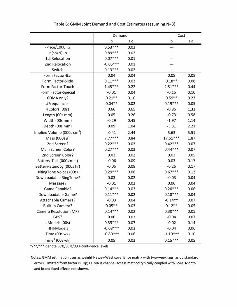
Table 6 displays the jointly estimated demand and cost parameters under our preferred

= 3 assumption. The demand estimates are qualitatively similar to previous estimates

under the monopoly hypothesis, in that consumers prefer brands with touch screens (com-

30We attempted to allow for non-simultaneous regime switches (e.g., one retailer switches two weeks before

our retailer and another retailer switches two weeks after our retailer). This, however, proved an exercise

too far for our one-retailer dataset, and estimates were unsatisfactory.31These -firm results are sensitive to the choice of market size , but estimation using different assumed

values of indicates that our results regarding the switch parameter are robust.32This imprecision is a direct result of the fact that identification stems from variation in the choice sets

and there is insufficient variation on this margin in the last months of the sample.

24

pared to flip phones), heavier phones, main displays with color, second screens, more ringtone

voices, more game capabilities, built-in camera resolution, and more models evenly spread

out within a brand’s portfolio. These estimated consumer preferences with respect to form

and function (especially camera and playback) largely anticipate the introduction of smart

phones that follows our sample. The secular and linear decline in phone demand given fixed

characteristics is also again apparent.

With a plausible price coefficient in hand, we can now put the impacts of the switch

and counter relocations into some perspective. The additional demand that came from the

switch was utility-equivalent to a price decline of U246(=

) or about $30. Because

our essential symmetry assumption has the relocations occurring only to our retailer, the

relocations could steal customers from (and lose customers to) other retailers. Despite the

comparable estimated descriptive impacts of the switch and relocations, the estimated struc-

tural impacts of relocations are much smaller than those of the switch, equivalent to U128($16) price decline for the first relocation and U95 ($12) price increase for the second. Costestimates are also as expected. Brands’ marginal costs are estimated to be significantly

higher for main display color, playback quality, and game/camera features. As one would

suppose given the speed of technological progress in the industry, these marginal costs ex-

hibit a secular decline over the sample. Conditional on the same characteristics, estimates

indicate that the marginal cost of producing a phone falls by U533 ($66) over the first yearbut only U287 ($35) over the fourth.Why would consumers respond to a change in the vertical contract between the retailer

and manufacturers? Theory predicts that manufacturers under revenue sharing may (de-

pending on the particular contracted revenue shares) charge lower final prices than the re-

tailer would charge under linear pricing. We have, however, controlled for consumer reaction

to any price changes. We have established that available brands are essentially unchanged

by the switch. Perhaps an improvement in brand characteristics coincided with the switch.

Changes in brand-level characteristics, though, are explicitly included. We are left with the

conclusion that manufacturers responded to the channel switch by improving the consumer’s

experience in some way. Given the relatively constant size of sales staff, the two obvious can-

didates are improved customer service (which might include better inventory management

and fewer stockouts, as well as higher quality staffing) and more (or better targeted) ad-

vertising. As we cannot distinguish between these explanations, we will henceforth combine

them into a generic customer service category.

25

Despite the structural foundation on which it was built, the above is essentially a reduced

form result, as it abstracts away from the mechanisms by which firms provide customer

service. We attempted the (heroic) task of estimating a model of demand in which consumers

respond to (unobserved) brand-specific customer service expenditures and those expenditures

are derived from profit-maximization conditions.33 In this case, the variable serves

as an instrument for the endogenous customer service variable. Estimates from such a model

could then be used to calculate the profit-maximizing expenditures on customer service under

any vertical contract and thus total profits (rather than variable profits) could be inferred.

While point estimates were significant and had the expected signs, magnitudes were highly

sensitive to the particular functional form by which customer service entered utility, and we

are unfortunately unable to make any robust claims from this approach.

5 Counterfactuals and welfare estimates

Using these estimates from our = 3 assumption, we now present five cases for the sam-

ple period after all retailers shifted from retailer-managed retailing with linear pricing to

manufacturer-managed retailing with revenue sharing (i.e., the last 34 weeks of 2006). In

each case, we use the inferred mean utilities without the price effects and marginal costs to

calculate the appropriate equilibrium prices and quantities using contraction mappings that

satisfy the first order necessary conditions. Specifically, for linear pricing, we use two nested

contraction mappings. Conditioning on specific wholesale prices, the interior routine is a

contraction mapping of own-retailer and other-retailer prices to the own-retailer and other-

retailer profit-maximization conditions. The outer routine then uses the comparative statics

implied by Cramer’s Rule and retailer first order conditions for a contraction mapping of

wholesale prices on manufacturer profit-maximization conditions. For revenue sharing, there

is a single contraction mapping of manufacturers’ own-retailer and other-retailer prices to

the manufacturers’ own-retailer and other-retailer profit-maximization conditions.

Means and standard errors of these implied prices and total quantities for our observed

retailer and other hypothetical retailers before and after the second relocation can be found

in Table 7. We then report industry cumulative variable profits captured by all retailers and

manufacturers as well as projected consumer surplus and welfare (sum of variable profits

and consumer surplus) in Table 8. Retailer ’s profits in each week are characterized as

33This is similar in spirit to Thomadsen (2005), in which unobserved quantities are inferred from observed

prices and profit-maximization conditions.

26

=

X=1

( −) , and manufacturer profits are =

¡ −

¢ X=1

We consider

variable profits in order to be consistent with the previous model, as retail costs (e.g., staffing)

are assumed to appear as fixed costs rather than variable.

Because our regime shift is market-wide and will presumably generate new equilibrium

prices across all retailers and brands, our measure of consumer surplus corresponds to the

hypothetical amount that consumers would pay for the entire retail mobile phone market to

exist at equilibrium prices. Referring to the expenditure function from classical consumer

theory and exploiting the assumption of no wealth effects in consumer demand for mobile

phones, (11 12 ) = (∞∞ ∞)− (11 12 ). We operationalize this

by sequentially increasing each brand-retailer’s price by U40 ($5) from its equilibrium price

and calculating consumer surplus until the brand-retailer’s choke-price is reached. That

brand-retailer’s price is then held at infinity, and the next brand-retailer is considered.34

Finally, while quality of customer service is presumably an endogenous and continuous vari-

able, we simplify the counterfactuals by imagining customer service as being either high (as

it was after the channel switch) or low (as it was before the switch). Standard errors are

calculated using finite perturbation and the delta method.

Case 1 reflects the actual manufacturer-managed retailing with revenue sharing. These

numbers therefore match the price-quantity observations of our retailer but reflect estimates

for other retailers’ prices and quantities, as well as variable profits, consumer surplus, and

welfare. Case 2 posits the counterfactual scenario that no retailers implemented the vertical

contracting change and that instead brands through the end of the sample were sold every-

where under the original regime of retailer-managed retailing with linear pricing. Cases 3

and 4 consider the counterfactuals of retailer-managed retailing with linear pricing and high

customer service and of manufacturer-managed retailing with revenue sharing and low cus-

tomer service. The final scenario (Case 5) considers the projected outcome if all retailers

had leased space to manufacturers for a fixed amount of rent rather than a share of revenue.

We set that rent amount to be roughly comparable to cumulative retailer variable profits

under the observed revenue-sharing agreement.

The features of the regime switch and the nested logit specification generate some unex-

pected outcomes that warrant upfront discussion. First, the revenue-shares returned to the

retailer are sufficiently large (over 20%) that competition among manufacturers is greatly

34Our use of the logit with its ready substitution across brands and retailers ensures that most of the

market’s consumer surplus is derived from the first brand-retailer phone being sold at the observed price.

27

dampened. When approached from the perspective of a standard pricing model, this leads

to the superficial appearance that manufacturers are leaving profits on the table by not

undercutting rivals’ prices. Second, the severe estimated inside-outside segmentation and

large implied probability of no purchase jointly generate the result that quantities expand

while firms’ prices are virtually unaffected by shocks that symmetrically affect all firms (e.g.,

switch that yields higher service quality). The graphical intuition from linear demand and

cost therefore does not apply.35

The implied prices and quantities of Table 7 show that linear pricing generates notably

higher prices than revenue sharing (Cols. (1) vs. (4) and Cols. (2) vs. (3)). Focusing

on the overall average weekly quantity sold (), the gain in units sold from the regime

switch (Cols. (2) vs. (1)) appear to come almost entirely from the increase in customer

service quality rather than the change from linear pricing to revenue sharing. The extreme

inside-outside segmentation is highlighted by the highly inelastic demand in this range of

prices. The relative importance of customer service and contract-type therefore stems at

least in part from our model’s lack of segmentation among inside options; consumers view

these brand-retailer options as close substitutes to each other. Moving away from revenue

sharing to simple rent (Cols. (1) vs. (5)) markedly lowers retail prices, as the positive

revenue shares faced by manufacturers dampened the payoffs of aggressive pricing. The

nested logit’s region of demand associated with such a price decline is much more elastic,

and this 10% price decline implies a 17% increase in quantity demanded. Standard errors of

this simple-rent counterfactual prices and quantities, however, are much larger.

Table 8 presents the variable profit, consumer surplus, and welfare implications (in thou-

sands of U) of these different regimes over the 34 weeks after the regime switch. Results arebroadly consistent with the story told by our managers, namely that retailers and manufac-

turers both benefited from the switch but that manufacturers’ gains were less. Given the fact

that staff-training costs are treated as fixed rather than variable, the relevant comparison

(Cols. (2) vs. (1)) understates the gains of the retailers and overstates those of the manu-

facturers. Consumers also markedly benefit from the switch, and consumer surplus rises by

15% and welfare by 17%. Both these level-increases are statistically significant (respective

t-stats of 6.8 and 9.0).

This comparison prompts the question of whether any cost advantage in staff-training by

manufacturers over retailers is required to explain the two aspects of our study. This could

35This result can also be shown numerically for nested-logit duopoly when inside-outside segmentation is

as severe ( ≈ 085) and the outside-option probability is as large (0 ≈ 095) as in our case.

28

alternatively be phrased as an investigation of retailers’ (manufacturers’) decision to provide

low (high) service quality before (after) the switch. Retail variable profits are estimated

to have risen by U3461K if retailers under linear pricing had provided high service qualityinstead of low service quality (Cols. (4) vs. (2)). This is a fixed cost within the model but,

when evaluated at the total quantity sold (averaged across the two hypothetical regimes),

works out to be approximately U38 ($4.7) per phone. The fact that retailers were notproviding high-quality service suggests that such service quality provision would have cost

retailers at least that amount. Likewise, manufacturer variable profits are estimated to have

risen by U1933K because manufacturers under revenue sharing provided high service qualityrather than low (Cols. (1) vs. (3)). This number then is an upper bound of what high

service quality provision cost manufacturers. Again evaluating at the average quantity sold

across the regimes, this yields U21 ($2.6) per phone.The relevant estimates are not calculated with sufficient precision to make any state-

ments with statistical confidence, but these results suggest a substantial cost advantage by

manufacturers in the provision of service quality. As previously discussed, this should come

as no surprise. Retailers in China’s one-megastore business culture lack the opportunities to

exploit scale economies in training when customer service quality is likely to be brand spe-

cific.36 Retailers in the Western economies with their multiple outlets may have such scale

opportunities, so we will defer on claiming that the service quality improvements observed in

our Chinese sample would also be generated by switches to manufacturer-managed retailing

in other countries.

None of the first four counterfactuals consider what might be the most obvious way to

sidestep the issues associated with vertical contracts, namely retailers charging manufacturers

fixed rent for the privilege of selling on the premises. We choose as our fixed rent an amount

that approximates the retailer profits under the original regime of linear pricing. Table 8’s

Col. (5) confirms the intuition that such a shift would be welfare-enhancing but also displays

why bargaining among manufacturers and retailers is unlikely to reach such an outcome. As

expected, consumer surplus is much higher (17%) under this straight-rent scenario than under

the hi-service quality/revenue-sharing scenario. Welfare, however, rises only modestly (3%),

as retailer profits fall slightly and manufacturers take a modest loss. This unusual result

is driven by the very high degree of segmentation between the inside and outside options

36This is also consistent with the idea that manufacturer-managed retail might make feasible the provision

of the full-line of products when costs of doing so under retailer-manged retailing would be prohibitive.

29

(i.e., close to 1).37 When our manufacturers exchange a variable cost (here the share

of revenues) for a fixed cost, their higher retained percentage of revenue incentivizes them

to compete more vigorously. This new Bertrand-like equilibrium yields outcomes at which

they are strictly worse off. Just as the portfolio effects of the retailer under linear pricing

retard fierce price-competition across brands, so too do the revenue shares. As this sharper

competition lowers the industry profits to be divided among retailers and manufacturers,

markets with many sellers of differentiated products are unlikely to evolve in this direction.

Conditioning estimation on assumed market structure is one of our more restrictive as-

sumptions, and so we also explore the implications of assuming = 4 retailers instead of

= 3. Recall from Table 5 that increasing the number of other retailers improved the match

between demand-alone and demand under joint estimation but also inflated the estimated

impact of the regime switch. Our counterfactuals for = 4 in the lower panel of Table 8

clearly reflect the latter point. The channel switch is estimated to have increased welfare by

22% instead of the 17% increase under the = 3 assumption. As joint estimation yielded

unsatisfactory matches with demand-alone estimation for the = 1 and = 2 cases,

we conclude that the above implications under the = 3 case are the most conservative

available.

6 Conclusions

In this paper, we consider how channel switches that shift retail responsibilities from retailers

to manufacturers affect customer service quality and ultimate market outcomes. Our results

show that manufacturers taking on responsibilities traditionally borne by retailers leads to

improved retail customer service. Customers benefit substantially from the channel switch

not only because of lowered prices but also because of this improved service. As such, this

paper is the first empirical study in the vertical-relationship literature to consider non-price

impacts in the context of retailers selling goods of several manufacturers. To this end, it

complements the fact that companies have long acknowledged that customers respond not

only to features and price but also a seller’s service effort (Rust and Chung, 2006). It also

contributes to the nascent body of rigorous empirical studies that document the importance

of service effort (e.g., Kim, 2014).

To the extent that such shifts continue and manufacturers take on responsibilities tradi-

tionally borne by retailers, our results suggest that consumers can benefit substantially. This

37Rey and Stiglitz (1995) derive a similar result after assuming perfectly inelastic market demand.

30

particular result of course hinges on much institutional detail, but our counterfactuals indi-

cate that manufacturers have a sizable cost advantage over retailers in the provision of high

service quality. The U.S. cosmetics industry with its tradition of revenue-sharing contracts

again comes to mind as exhibiting these same features.

While we believe our identification assumptions to be sound, the credibility of our core re-

sult (demand increasing under manufacturer-provided customer service) would be enhanced

by applications and tests that were able to use a different identification strategy. Many

channel changes have been observed in recent years. They may offer the opportunity for

datasets that sidestep some of the concerns that our data and setting raised. To the extent

that the analyst can control for institutional features, further research may be able to more

conclusively illuminate our findings.

One natural extension of this work is to consider the optimality of our retailer’s choice of

revenue shares. Higher revenue shares will presumably harm consumers through higher retail

prices, but it is possible that industry profits would rise as competition among manufacturers

is further dampened. Another extension gets back to our primary interest of vertical con-

tracts and customer service. Our inferences on retailer and manufacturer profits were limited

by the lack of data regarding expenditures on staffing and customer service, but analysis of

more detailed data on those margins could reveal the mechanism by which customer ser-

vice improves. Given the global importance of the retail sector, additional attention to this

contractual switch is warranted.

References

[1] Ascarza, Eva, Anja Lambrecht and Naufel Vilcassim. 2012. “When Talk is ‘Free’: An

Analysis of Subscriber Behavior Under Two- and Three-Part Tariffs,” Journal of Mar-

keting Research, 49(6): 882-99.

[2] Berry, Steven. 1994. “Estimating Discrete Choice Models of Product Differentiation,”

RAND Journal of Economics, 25(3): 242-62.

[3] ––, James Levinsohn, and Ariel Pakes. 1995. “Automobile Prices in Market Equilib-

rium,” Econometrica, 60(4): 889-917.

[4] ––, and Joel Waldfogel. 1999. “Free Entry and Social Inefficiency in Radio Broadcast-

ing,” RAND Journal of Economics, 33(3): 397-420.

31

[5] Bonnet, Celine, and Pierre Dubois. 2010. “Inference on Vertical Contracts betweenMan-

ufacturers and Retailers Allowing for Nonlinear Pricing and Resale Price Maintenance,”

RAND Journal of Economics, 41(1): 139-64.

[6] Cachon, Gerard P., and Martin A. Lariviere. 2004. “Supply Chain Coordination with

Revenue-Sharing Contracts,” Management Science, 51(1): 30-44.

[7] Chen, Chia-Wen. 2014. “Estimating the Foreclosure Effect of Exclusive Dealing: Ev-

idence from Entry of Specialty Beer Producers,” International Journal of Industrial

Organization (forthcoming).

[8] Chen, Xinlei, George John, & Om Narasimhan. 2008. “Assessing the Consequences of

a Channel Switch,” Marketing Science, 27(3): 398-416.

[9] Conlon, Christopher T., and Julie H. Mortimer. 2014. “Efficiency and Foreclosure Effects

of All-Units Discounts: Empirical Evidence,” manuscript, Boston College.

[10] Dana, James D., Jr., and Kathryn E. Spier. 2001. “Revenue Sharing and Vertical Control

in the Video Rental Industry,” Journal of Industrial Economics, 49(3): 223-45.

[11] Desai, Preyas, and Kannan Srinivasa. 1995. “Demand Signalling Under Unobservable

Effort in Franchising: Linear and Non-Linear Contracts,” Management Science, 41(10):

1608-23.

[12] Einav, Liran. 2007. “Seasonality in the U.S. Motion Picture Industry,” RAND Journal

of Economics, 38(1): 127-45.

[13] Ferrari, Stijn, and Frank Verboven. 2012. “Vertical Control of a Distribution Network -

An Empirical Analysis of Magazines,” RAND Journal of Economics, 43(1): 26-50.

[14] Ho, Justin, Katherine Ho, and Julie H. Mortimer. 2012. “The Use of Full-Line Forcing

Contracts in the Video Rental Industry,” American Economic Review, 102(2): 686-719.

[15] Jerath, Kinshuk, and Z. John Zhang. 2010. “Store-Within-a-Store,” Journal of Market-

ing Research, XLVII (August), 748-63.

[16] Kadiyali, Vrinda, Pradeep Chintagunta & Naufel Vilcassim. 2000. “Manufacturer-

Retailer Channel Interactions and Implications for Channel Power: An Empirical In-

vestigation of Pricing in a Local Market,” Marketing Science, 19(2): 127-48.

32

[17] Kim, Stephen K., Richard G. McFarland, Soongi Kwon, Sanggi Son, and David A.

Griffith. 2011. “Understanding Governance Decisions in a Partially Integrated Channel:

A Contingent Alignment Framework,” Journal of Marketing Research, 48(3): 603-16.

[18] Kim, Tongil. 2014. “When Franchisee Service Effort Affects Demand: An Application

to the Car Radiator Market and Resale Price Ceiling,” manuscript, Emory University.

[19] Lafontaine, Francine and Margaret Slade. 1997. “Retail Contracting: Theory and Prac-

tice,” Journal of Industrial Economics, 45(1): 1-25.

[20] –– and ––. 2008. “Exclusive Contracts and Vertical Restraints: Empirical Evidence

and Public Policy,” in Handbook of Antitrust Economics, ed. Paolo Buccirossi, MIT

Press.

[21] Liu, Qihong, and Jie Shuai. Forthcoming. “Reverse Pricing and Revenue Sharing in a

Vertical Market,” Managerial and Decision Economics.

[22] Manuszak, Mark. 2010. “Predicting the Impact of Upstream Mergers on Downstream

Markets with an Application to the Retail Gasoline Industry,” International Journal of

Industrial Organization, 28 (1): 99-111.

[23] McFadden, Daniel. 1978. “Modelling the Choice of Residential Locations,” in A. Kar-

lqvist et al., eds., Spatial Interaction Theory and Planning Models, Amsterdam: North-

Holland Publishing.

[24] Mortimer, Julie H. 2008. “Vertical Contracts in the Video Rental Industry,” Review of

Economic Studies, 75: 165-99.

[25] Moul, Charles C. 2008. “Retailer Entry Conditions and Wholesaler Conduct: The the-

atrical distribution of motion pictures,” International Journal of Industrial Organiza-

tion, 26(4): 966-84.

[26] ––. 2012. “A New Test for Monopoly with Limited Cost Data,” Economic Letters,

117: 891-4.

[27] Rey, Patrick, and Joseph Stiglitz. 1995. “The Role of Exclusive Territories in Producers’

Competition,” RAND Journal of Economics, 26 (3): 431-51.

33

[28] Rust, Roland T., and Tuck Siong Chung. 2006. “Marketing models of service and rela-

tionships,” Marketing Science, 25(6): 560-80.

[29] Sudhir, K. 2001. “Structural Analysis of Manufacture Pricing in the Presence of a

Strategic Retailer,” Marketing Science, 20(3): 244-64.

[30] Thomadsen, Raphael. 2005. “The Effect of Ownership Structure on Prices in Geograph-

ically Differentiated Industries,” RAND Journal of Economics, 36(4): 908-29.

[31] Tirole, Jean. 1988. The Theory of Industrial Organization. The MIT Press: Cambridge,

MA.

[32] Villas-Boas, J. Miguel and Ying Zhao. 2005. “Retailer, Manufacturers, and Individ-

ual Consumers: Modeling the Supply Side in the Ketchup Marketplace,” Journal of

Marketing Research, Vol. XLII (February 2005): 83-95.

[33] Villas-Boas, Sofia. 2007. “Vertical Relationships between Manufacturers and Retailers:

Inference with Limited Data,” Review of Economic Studies, 74: 625-52.

[34] ––. 2009. “An Empirical Investigation of the Welfare Effects of Banning Wholesale

Price Discrimination,” RAND Journal of Economics, 40 (1): 20-45.

[35] Wu, X. 2005. “A Survey of the Department Store Selling Mechanism,” Business Time,

27.

[36] Xiao, Ping, Tat Chan, and Chakravarthi Narasimhan. 2008. “Product Bundling under

Three-Part Tariffs in the Wireless Industry,” Working paper, SSRN 1125209.

34

                                        Table 1: Quantity, Price, and Revenue Shares by Brand

             Weekly Quantity MktSh              Weekly Price (RMB) RevSh

Brand Mean SD Min Max Mean Mean SD Min Max % to Ret

Nokia 289.50 58.55 128 519 19.46% 1616 260 1042 3547 22.5

Motorola 252.38 80.62 73 669 17.90% 1755 332 1199 2753 22.5

Bird 151.81 46.31 76 371 12.83% 1066 177 685 1545 25.0

Samsung 148.00 37.28 84 297 12.03% 2408 277 1799 3263 22.5

Sony Ericsson 89.77 45.53 21 285 6.76% 1941 358 804 2694 22.5

TCL 73.23 22.44 7 164 6.18% 1246 169 858 1751 26.0

Konka 58.72 28.53 14 252 4.58% 1155 213 595 1688 26.0

NEC 53.77 23.05 15 128 4.21% 2378 795 814 4818 25.0

Siemens/Asus 43.48 38.87 3 238 3.27% 1489 260 744 2363 22.5

Philips 34.47 15.32 5 92 2.13% 1591 186 1007 1998 26.0

TELSDA 32.83 14.56 8 109 1.88% 1198 200 744 1679 26.0

CECT 31.80 18.52 7 105 1.40% 1550 270 850 2593 26.0

Overall 92.63%

Notes: Market shares taken directly from retailer and include sales of brands not shown. Weekly prices are calculated as 

    weekly brand revenues divided by weekly brand units sold and are denominated in renminbi (yuan). During our sample 

    period, the exchange rate between the RMB and US$ is about 8.1:1. RevSh denotes the share of revenue retained by the 

    retailer after the switch to retailing by manufacturers.

                     Table 2: Brand‐Level Product Characteristics

Mean SD Min Max

Form Factor‐Bar 0.36 0.34 0 1

Form Factor‐Slide 0.06 0.14 0 1

Form Factor‐Touch 0.01 0.02 0 0.23

Form Factor‐Special 0.03 0.11 0 1

CDMA only? 0.01 0.04 0 0.42

#Frequencies 2.32 0.37 1.61 3.45

#Colors 2.34 0.64 1.00 5.25

Length (mm) 92.46 7.54 49.50 110.00

Width (mm) 45.22 2.57 35.72 91.00

Depth (mm) 20.62 2.12 10.80 27.20

Implied Volume (cm3) 85.74 11.26 48.38 145.65

Mass (g) 87.50 7.33 64.00 122.84

2nd Screen? 0.45 0.34 0 1

Main Screen Color? 0.81 0.28 0 1

2nd Screen Color? 0.16 0.21 0 1

Battery‐Talk (min) 272.83 110.10 65.56 706.83

Battery‐Standby (hr) 225.66 120.22 74.92 822.00

#RingTone Voices 33.02 16.70 1.00 73.85

Downloadable RingTone? 0.84 0.21 0 1

Message? 0.71 0.29 0 1

Game Capable? 0.93 0.12 0.13 1

Downloadable Game? 0.45 0.34 0 1

Attachable Camera? 0.08 0.16 0 0.89

Built‐In Camera? 0.49 0.36 0 1

Camera Resolution (MP) 0.33 0.41 0 2.27

GPS? 0.06 0.13 0 1

#Models 13.33 8.94 1 46

HHI‐Models 0.19 0.15 0.03 1

Notes: Omitted Form Factor is Flip (Clamshell); CDMA is a channel access method 

     that is typically coupled with GSM

                        Table 3: Quantity and Price by Sample Period

All I II III IV

Q Mean 104.98 104.72 107.74 114.53 88.64

SD 93.44 95.17 95.69 88.52 75.52

Min 3 7 3 7 4

Max 669 669 556 384 308

P (RMB) Mean 1616 1699 1566 1401 1395

SD 541 590 430 412 455

Min 595 744 744 595 685

Max 4818 4818 3584 2432 2676

n 2496 1452 636 204 204

I: Before 1st relocation (Wks 1‐121)

II: After 1st relocation but before Switch (Wks 122‐174)

III: After Switch but before 2nd relocation (Wks 175‐191)

IV: After 2nd relocation (Wks 192‐208)

Notes: Weekly prices denominated in renminbi. During our sample period, the exchange

    rate between the RMB and US$ is about 8.1:1

   Table 4: OLS Descriptive Estimation Results of Brand Weekly Variables (n=2496)

    DepVar ‐ Quantity DepVar ‐ Price (RMB)

b s.e. b s.e.

Switch 25.46*** 7.73 ‐15.22 42.54

1st Relocation 24.47*** 5.87 72.39** 35.87

2nd Relocation ‐26.11*** 5.94 9.44 30.36

Form Factor‐Bar 7.64 10.46 ‐12.56 92.46

Form Factor‐Slide 1.98 10.08 179.75** 83.71

Form Factor‐Touch ‐252.78*** 112.40 2204.22*** 451.35

Form Factor‐Special 12.34 11.05 ‐196.83* 117.57

CDMA only? ‐85.21** 42.36 463.55* 251.00

#Frequencies ‐25.01*** 6.32 188.13*** 54.73

#Colors 4.88** 1.92 ‐5.23 13.54

Length (mm) 2.00*** 0.75 ‐0.28 6.44

Width (mm) 2.81** 1.15 ‐9.44 12.62

Depth (mm) 5.89** 2.65 ‐8.89 24.58

Implied Volume (10 cm3) ‐11.62* 6.38 ‐13.54 61.39

Mass ‐1.19*** 0.25 17.87*** 2.18

2nd Screen? 2.44 7.30 390.69*** 75.77

Main Screen Color? ‐3.71 8.75 593.81*** 76.26

2nd Screen Color? 7.46 5.39 ‐0.17 59.38

Battery‐Talk (00s min) ‐9.12 27.07 ‐190.68 190.70

Battery‐Standby (00s hr) 69.05*** 22.71 1.93 179.81

#RingTone Voices ‐0.19 0.17 3.56** 1.40

Downloadable RingTone? 1.62 6.32 5.71 43.95

Message? ‐9.97 5.36 51.56 42.32

Game Capable? ‐22.09*** 7.78 178.09*** 64.17

Downloadable Games? 2.84 4.33 181.76*** 43.52

Attachable Camera? 13.22 9.88 ‐229.01*** 75.15

Built‐In Camera? ‐2.82 6.47 127.57** 60.37

Camera Resolution (MP) ‐6.75 4.96 297.38*** 55.82

GPS? 14.97** 6.95 51.38 79.02

#Models ‐0.42 0.26 0.15 1.33

HHI‐Models ‐28.85*** 7.66 ‐63.14 69.82

Time (00s wk) 16.88 15.96 ‐1109.83*** 124.62

Time2 (00s wk) ‐11.27 9.21 130.09* 67.53

R2

0.8548 0.8657

F‐stat on IVs

3.14 4.45

         */**/*** denote 90%/95%/99% confidence levels

Notes: Quantities are in singleton units, prices are in RMB. Regressions also include brand fixed effects and 

    month fixed effects; omitted form factor is Flip; CDMA is a channel access method typically coupled with GSM. 

    Standard errors reflect inefficient estimation and Newey‐West correction with two‐week lag.

 Test of null hypothesis that IVs have no predictive power beyond above regressors. F‐stat 99% confidence     threshold is 1.7.

               Table 5: Stand‐Alone and Joint‐with‐Cost GMM Demand Estimates & Implications under various N‐firm assumptions

           N=1            N=2            N=3            N=4            N=5            N=6            N=8

Alone Joint Alone Joint Alone Joint Alone Joint Alone Joint Alone Joint Alone Joint

‐Price/1000:  0.35 1.48 0.39 0.51 0.39 0.53 0.40 0.54 0.40 0.55 0.41 0.55 0.42 0.57

(0.08) (0.05) (0.07) (0.02) (0.07) (0.02) (0.08) (0.03) (0.08) (0.03) (0.08) (0.03) (0.08) (0.03)

ln(sh/N):  0.85 1.00 0.84 0.93 0.84 0.89 0.84 0.87 0.84 0.86 0.83 0.85 0.83 0.84

(0.06) (0.14) (0.06) (0.02) (0.06) (0.02) (0.06) (0.03) (0.06) (0.03) (0.06) (0.03) (0.06) (0.03)

Switch 0.23 0.20 0.12 0.03 0.16 0.13 0.19 0.17 0.21 0.19 0.23 0.21 0.24 0.23

(0.02) (0.17) (0.04) (0.02) (0.03) (0.02) (0.03) (0.02) (0.02) (0.02) (0.02) (0.02) (0.02) (0.02)

1st Relocation 0.24 0.34 0.12 0.09 0.08 0.07 0.07 0.06 0.06 0.06 0.05 0.06 0.05 0.05

(0.02) (0.12) (0.02) (0.01) (0.02) (0.01) (0.02) (0.01) (0.02) (0.01) (0.02) (0.01) (0.02) (0.01)

2nd Relocation ‐0.25 ‐0.22 ‐0.09 ‐0.06 ‐0.07 ‐0.05 ‐0.06 ‐0.05 ‐0.06 ‐0.05 ‐0.05 ‐0.05 ‐0.05 ‐0.05

(0.02) (0.66) (0.02) (0.01) (0.02) (0.01) (0.02) (0.01) (0.02) (0.01) (0.02) (0.01) (0.02) (0.01)

ObjFunc 5.30 20.79 198.50 325.93 196.62 316.57 195.26 311.15 195.97 308.12 196.05 305.94 196.13 303.18

Hausman N/A 10.10 7.53 6.75 6.36 6.15 5.94

Hausman p ‐‐‐ 0.006 0.023 0.034 0.042 0.046 0.051

E(D) ‐3.49 ‐10928 ‐3.81 ‐10.84 ‐3.87 ‐7.58 ‐3.86 ‐6.67 ‐3.92 ‐6.27 ‐3.96 ‐6.04 ‐4.00 ‐5.78

E(wp) ‐1264 975 924 1373 1076 1352 1128 1348 1179 1346 1202 1345 1217 1345

#wp<0 2018 0 6 0 0 0 0 0 0 0 0 0 0 0

E(mc|Switch=0) ‐1729 975 483 1218 637 1127 684 1092 739 1071 766 1059 723 1046

E(mc|Switch=1) 708 1059 737 945 743 898 743 877 748 864 751 857 754 848

#mc<0 2061 0 341 0 143 0 94 0 51 0 35 0 31 0

 Because of collinearity issues with the Newey‐West correction, the N=1 case displays 2SLS estimates with robust standard errors rather than GMM.

Notes: Standard errors in parentheses and reflect Newey‐West correction with two lags. Regressions also include product characteristics, quadratic time‐trends, brand

    fixed effects and month fixed effects). Hausman test based on difference between stand‐alone and joint estimates of only price and market share coefficients (, ).    Implied wholesale prices and marginal costs in RMB.

                      Table 6: GMM Joint Demand and Cost Estimates (assuming N=3)

          Demand                Cost

b s.e. b s.e.

‐Price/1000:  0.53*** 0.02 ‐‐‐

ln(sh/N):  0.89*** 0.02 ‐‐‐

1st Relocation 0.07*** 0.01 ‐‐‐

2nd Relocation ‐0.05*** 0.01 ‐‐‐

Switch 0.13*** 0.02 ‐‐‐

Form Factor‐Bar 0.04 0.04 0.08 0.08

Form Factor‐Slide 0.11*** 0.03 0.18** 0.08

Form Factor‐Touch 1.45*** 0.22 2.51*** 0.44

Form Factor‐Special ‐0.01 0.04 ‐0.15 0.10

CDMA only? 0.21** 0.10 0.59** 0.23

#Frequencies 0.04** 0.02 0.19*** 0.05

#Colors (00s) 0.66 0.65 ‐0.85 1.33

Length (00s mm) 0.05 0.26 ‐0.73 0.58

Width (00s mm) ‐0.29 0.45 ‐1.97 1.14

Depth (00s mm) 0.09 1.04 ‐3.31 2.21

Implied Volume (000s cm3) ‐0.41 2.44 5.63 5.51

Mass (000s g) 7.77*** 0.84 17.51*** 1.87

2nd Screen? 0.22*** 0.03 0.42*** 0.07

Main Screen Color? 0.27*** 0.03 0.44*** 0.07

2nd Screen Color? 0.03 0.02 0.03 0.05

Battery‐Talk (000s min) ‐0.06 0.09 0.03 0.17

Battery‐Standby (000s hr) ‐0.05 0.08 ‐0.25 0.17

#RingTone Voices (00s) 0.29*** 0.06 0.67*** 0.12

Downloadable RingTone? 0.03 0.02 ‐0.03 0.04

Message? ‐0.01 0.02 0.06 0.04

Game Capable? 0.14*** 0.03 0.20*** 0.06

Downloadable Game? 0.11*** 0.02 0.18*** 0.04

Attachable Camera? ‐0.03 0.04 ‐0.14** 0.07

Built‐In Camera? 0.05** 0.03 0.12** 0.05

Camera Resolution (MP) 0.14*** 0.02 0.30*** 0.05

GPS? 0.00 0.03 ‐0.04 0.07

#Models (00s) 0.35*** 0.07 ‐0.02 0.14

HHI‐Models ‐0.08*** 0.03 ‐0.04 0.06

Time (00s wk) ‐0.80*** 0.06 ‐1.10*** 0.10

Time2 (00s wk) 0.05 0.03 0.15*** 0.05

           */**/*** denote 90%/95%/99% confidence levels

Notes: GMM estimation uses as weight Newey‐West covariance matrix with two‐week lags, as do standard 

    errors. Omitted form factor is Flip; CDMA is channel access method typically coupled with GSM. Month 

    and brand fixed effects not shown.

               Table 7: Counterfactual Outcomes during Post‐Switch Period (assumes N=3)

(1) Reality (2) No change (3) Only Contract (4) Only Service (5) Rent

Contract†

RS‐MMR LP‐RMR RS‐MMR LP‐RMR Rent‐MMR

Service Hi Lo Lo Hi Hi

E(p11) 1429

1618 1429 1618 1279

(32) (36) (32) (36) (164)

E(p21) 1424 1566 1424 1566 1276

(33) (32) (33) (32) (162)

E(p*1) 1427 1588 1427 1588 1277

(33) (34) (33) (34) (163)

E(p12) 1424

1618 1424 1618 1305

(39) (33) (39) (33) (131)

E(p22) 1423 1605 1423 1605 1304

(39) (33) (39) (33) (130)

E(p*2) 1423 1610 1423 1610 1304

(39) (33) (39) (33) (130)

E(p) 1425 1599 1425 1599 1291

(34) (32) (34) (32) (146)

E(wp) ‐‐‐ 1300 ‐‐‐ 1300 ‐‐‐

(30) (30)

E(q11) 1374

1059 1211 1202 1601

(34) (26) (45) (21) (245)

E(q21) 764 734 673 833 892

(36) (17) (39) (10) (120)

E(q*1) 967 842 852 956 1128

(31) (17) (38) (8) (161)

E(q12) 1064

899 937 1020 1242

(32) (25) (39) (22) (196)

E(q22) 916 816 807 926 1070

(38) (19) (42) (10) (150)

E(q*2) 965 844 850 957 1128

(30) (18) (37) (9) (164)

E(q) 966 843 851 956 1128

(30) (17) (37) (7) (162)

Total Q sold 98549 85971 86845 97557 115051

(3060) (1745) (3797) (758) (16566)

†: Compensa on (RS ‐ revenue‐sharing, LP ‐ linear pricing, Rent ‐ simple rent) & Retail‐responsibility

Notes: Standard errors in parentheses beneath estimates,  matches mean from data. First subscript references retailer

    (1‐observed, 2‐other). Second subscript references before 2nd relocation (1) and after (2). All retail and wholesale price 

    averages reflect weighting by market shares conditional on purchase within week and then average across relevant

    weeks. All prices in RMB.

           Table 8: Profit, Consumer Surplus, and Welfare Estimates during Post‐Switch Period 

(1) Reality (2) No change (3) Only Contract (4) Only Service (5) Rent

Contract Type†

RS‐MMR LP‐RMR RS‐MMR LP‐RMR Rent‐MMR

Service Hi Lo Lo Hi Hi

N=3

Retail  32845 25648 28944 29109 30000

(1237) (4228) (1422) (4834) ‐‐‐

Manufacturer  16272 12415 14339 14091 ‐4969

(3025) (5288) (2821) (5849) (2467)

Consumer Surplus 189625 165186 166896 187680 221750

(3747) (6412) (3981) (8243) (38755)

Welfare 238742 203250 210179 230880 246782

(3777) (6428) (5998) (4292) (39728)

N=4

Retail  45266 34220 38302 40451 40000

(2054) (5476) (2066) (6188) ‐‐‐

Manufacturer  25223 20544 21343 24285 ‐1358

(4592) (7023) (4038) (9124) (3727)

Consumer Surplus 256446 212210 216511 251353 299430

(4259) (8086) (5259) (9740) (38742)

Welfare 326935 266974 276156 316089 338071

(6182) (8763) (8409) (6737) (38853)

†: Compensa on (RS ‐ revenue‐sharing, LP ‐ linear pricing, Rent ‐ simple rent) & Retail‐responsibility

Notes: Standard errors in parentheses beneath estimates. All figures reflect cumulative totals (in 1000 RMB) for all firms 

    (observed and assumed) over last 34 weeks of sample. Displayed profits are variable profits and do not reflect fixed costs 

    stemming from different service levels