Food Quality and Preference 31 (2014) 69–80

Contents lists available at ScienceDirect

Food Quality and Preference

journal homepage: www.elsevier .com/locate / foodqual

Why are discounted prices presented with full prices? The roleof external price information on consumers’ likelihood topurchase

0950-3293/$ - see front matter Crown Copyright � 2013 Published by Elsevier Ltd. All rights reserved.http://dx.doi.org/10.1016/j.foodqual.2013.08.003

⇑ Address: Department of Economics, University of Manchester, Oxford Road,Manchester M13 9PL, United Kingdom. Tel.: +44 (0) 161 306 6929.

E-mail address: luca.panzone@manchester.ac.uk

Luca A. Panzone ⇑Department of Economics and Sustainable Consumption Institute, University of Manchester, United Kingdom

a r t i c l e i n f o

Article history:Received 3 April 2013Received in revised form 26 July 2013Accepted 1 August 2013Available online 9 August 2013

Keywords:External Reference PricePrice–quality proxyDiscountsContingent valuationBivariate ordered probit

a b s t r a c t

Apart from being a cost, prices inform consumers on the quality of goods. To retain informative power,discounted prices are often presented together with their original value as an External Reference Price(ERP). Observing the impact of the ERP on consumer preferences using two contingent valuation surveysto wine consumers, the paper observes that the presence of both prices and ERPs guide consumer choices.In particular, ERPs shift the attention of consumers towards expensive products and high discounts, byproviding information on quality and allowing for time-efficient decisions. Results show that ERPs: (a)have a positive impact on preferences, but less (in absolute value) than prices; (b) stimulate the choiceof items with high price and large discounts; (c) make consumers revise their choices. The presence ofan ERP can, in certain conditions, lead to a positive response to high prices.

Crown Copyright � 2013 Published by Elsevier Ltd. All rights reserved.

1. Introduction

In modern markets consumers are often called to choose in con-ditions of risk and uncertainty about the intrinsic quality of goodsthey buy (Akerlof, 1970; Ariely & Norton, 2011). However, buyerscan use prices to determine the quality of goods and to rank differ-ent options by quality before a choice (Kirmani & Rao, 2000; Mon-roe, 1973; Rao, 2005; Rao & Monroe, 1989; Gerstner, 1985),assuming a positive price–quality correlation (Ding, Ross, & Rao,2010). This price–quality heuristic is based on the commonknowledge that high quality requires expensive inputs and canbe produced in limited quantity (Bagwell & Riordan, 1991). Fur-thermore, suppliers of high quality goods use high prices to signaltheir superior quality (Spence, 1973, 2002; Stiglitz, 1987) and cancount on future profits only if the high price-high quality relationtruly exists (Bagwell & Riordan, 1991; Cooper & Ross, 1984;Milgrom & Roberts, 1986).

While research has explored extensively this price–qualityproxy, there is little understanding of the cognitive distortion dis-counts may cause to the assumption of a positive price–qualitycorrelation (Palazon & Delgado-Ballester, 2009). For example, inthe occurrence of a temporary price change, a product worth £15and sold at £10 would be perceived to perform less well at the

discounted price compared to its full price if the latter is unknown.Any imperfect expectation should correct itself through repeatedconsumption, but quality distortions caused by price perceptionare not fully conscious (Plassmann, O’Doherty, Shiv, & Rangel,2008; Shiv, Carmon, & Ariely, 2005): they alter the experience per-formance of goods, limiting an effective learning process.

A common strategy to overcome this problem is to providequality cues. Retailers often provide consumers with External Ref-erence Prices (ERP) (Kalyanaram & Winer, 1995; Mazumdar, Raj, &Sinha, 2005). This piece of information refers to: the price of a di-rect substitute, referred to as a contextual reference price (Rajen-dran and Tellis, 1994), i.e. the price of a competing brand; or anadvertised reference price, i.e. the price of the same good in a dif-ferent location (e.g. a competing store), in a previous shopping trip(a temporal reference price), or from a different source (e.g. therecommended retail price) (Mazumdar et al., 2005). ERPs are calledexternal because they are not generated within the consumer’smind and represent pieces of information external to the bundleof attributes that are needed in a transaction (Mayhew & Winer,1992; Zeithaml, 1988; and Kopalle & Lindsey-Mullikin, 2003).

The primary objective of this article is to understand consumerbehaviour in the presence of an ERP. The literature on the subject iswell established (e.g. Mayhew & Winer, 1992; and Kopalle &Lindsey-Mullikin, 2003), but the mechanisms underlying theiruse are not yet fully understood. Current research indicates thatconsumers’ response to prices contains a significant behaviouralcomponent driven by a subjective cognitive interpretation of ERPs,

70 L.A. Panzone / Food Quality and Preference 31 (2014) 69–80

as well as feelings and emotions ERPs may evoke (Cheng & Monroe,2013; Thomas, 2013). Importantly, ERPs might induce an auto-matic consumer response, i.e. a positive prime, which makeschoices faster by reducing cognitive effort. Nevertheless, it remainsunclear whether ERPs direct and change consumer choices. To ex-plore this matter, this article estimates a utility function for wine, agood with high search costs, to understand whether choices withknowledge of an ERP differ from those without it. Using the samedataset, Panzone (2012) observes that exogenous changes in ERPalter the perceived quality of goods, but does not compare choiceswith and without ERPs.

Specifically, ERPs could cause an anchoring bias (Ariely, Loe-wenstein, & Prelec, 2003; Tversky & Kahneman, 1974), wherebyconsumers base their quality expectations on ERPs possibly per-ceiving them as more reliable than their own inference (see alsoKopalle, Kannan, Boldt, & Arora, 2012). Similarly, ERPs could causean attentional bias (Smith et al., 2006): by signalling quality, theymay make other pieces of information less relevant to the choicetask. Adaptation theory indicates that expectations over futureoutcomes depend on past experienced outcomes and current stim-uli (Chen, 2009), and because past hedonic performances uncon-sciously depend on ERPs (Plassmann, O’Doherty, Shiv, & Rangel,2008; Shiv et al., 2005) their presence is likely to reinforce a biasand make it automatic. The result of this inferential process maylead consumers to prefer an item when both expensive (i.e. highERP) and with a high discount (i.e. low price to pay), giving littleattention to other product characteristics.

Choices rely heavily on non-sensory information (Jaeger, 2006;Peri, 2006) such as contextual cues and marketing activities (Daw-son, 2013; Dhar & Novemsky, 2008), which are crucial in somewine segments (Lockshin, Jarvis, d’Hauteville, & Perrouty, 2006).ERPs anchor a consumer’s valuation to the extent that any priceinformation is assessed with respect to its original price. Economictheories of consumer behaviour allow for an impact of ERPs onchoices, but their presence would not be anticipated to affect pricesensitivity, because price alone determines the allocation ofmoney. Note that the ERP should be expected to restore the distor-tion of the price-quality proxy in the presence of discounts with anoverall neutral effect, and a high impact of ERPs on utility wouldentail consumers can be ‘‘nudged’’ into purchasing a good just byincluding an ERP.

A second objective is to understand how ERPs are used.Consumers use price to infer unobservable product quality (e.g.Kirmani & Rao, 2000; Monroe, 1973; Rao, 2005). However, pricesmay become (partially or fully) uninformative when an ERP ispresent, because quality is now communicated by another source.Furthermore, consumers gain positive feelings from the knowledgeof a discount, and the ERPs make this monetary reward salient(Kopalle & Lindsey-Mullikin, 2003; Mayhew & Winer, 1992).Knowledge of the discount then reduces the importance of the costcomponent of price, reducing price sensitivity. A final objective isto observe whether the presence of ERPs changes consumerchoices. By comparing consumers’ responses in the two CV sur-veys, it is possible to examine whether the same respondent re-vises her choice when the ERP is known. Data indicate 36% ofconsumers changed their initial decision, and inconsistency is afrequent outcome. Consumers revised their utility downwardsmore frequently than upwards, depending on the position of pricerelative to the ERP.

These research questions are explored through two contingentvaluation (CV) surveys to wine consumers. Albeit rarely used formarket goods (e.g. Park & MacLachlan, 2008), this technique isrecognised as reliable in the determination of consumerpreferences (Alberini, Boyle, & Welsh, 2003; Carson, Flores, &Meade, 2001; Hanemann, 1984; Wang, 1997). The use of statedpreferences allows estimating a utility function for wine removing

the collinearity between price and ERP, and the possible endogene-ity of discounts. In the first CV survey, respondents indicated theirintention to purchase an existing wine at a given randomlyallocated price. In the second survey, respondents repeated thetask in the presence of an advertised ERP. Because CV responsesare not fully incentive-compatible (Wertenbroch & Skiera, 2002),results are compared to estimates from revealed preference.

The remainder of the paper is as follows. Section 2 introducesthe econometric model used in the empirical analysis. Section 3presents the data collection process. The case study focuses onthe wine market because of its highly differentiated supply, andcommon use of price as quality proxy (Chaney, 2000; Drummond& Rule, 2005; Mitchell & Greatorex, 1989; Ritchie, 2007). Further-more, wine choices appear to be made in condition of risk anduncertainty over intrinsic quality (Drummond & Rule, 2005; Mitch-ell & Greatorex, 1989), making the context suitable for the pur-poses of this study. Results are presented in Section 4, whileSection 5 discusses the findings of the article and concludes.

2. Econometric model

The present section incorporates the ERP into a simple economicmodel of choice. In the market, a consumer j with income Yj is ex-pected to purchase a wine i with characteristics Xi sold at a marketprice Pi only if he expects a positive utility from the intrinsic qualityof the good, Si. The utility of the consumer corresponds to

Uij ¼ UðSiÞ ð1Þ

Si is unknown to consumers, and choices are risky and lead touncertain outcomes, particularly in information intensive markets.Consumers will then infer Si on the basis of information available.

2.1. Only price available

In the absence of an objective measure of Si, consumersestimate quality on the basis of observable characteristics(Broniarczyk & Alba, 1994) and price (Rao, 2005), through a subjec-tive process (Alba & Hutchinson, 2000). The estimated Sij can bespecified as

Sij ¼ gðXi; Pi;DjÞ ð2aÞ

where Dj are demographics. The resulting utility function can thenbe written as

Uij ¼ bo þ b1 � Xi þ b2 � Dj þ b3 � Pi þ b4 � Yj þ gij ð3aÞ

where gij are normally distributed residuals. The coefficient of price(b3) in Eq. (3a) refers to the utility of price as a cost, dC , and as infor-mation about product quality, dI , so that b3 ¼ ðdI þ dCÞ. A negative b3

indicates that the absolute value of the cost element is larger thanthe informational one. Conversely, the price coefficient is positivewhenever price as information is more important than price as acost (Basmann, Molina, & Slottje, 1988; Leibenstein, 1950; Veblen,1998). Finally, the equality jdC j ¼ jdIj implies b3 ¼ 0, a condition thatcan be misinterpreted with price non-attendance (Scarpa, Gilbride,Campbell, & Hensher, 2009).

2.2. Price and ERP available

Imagine now consumer j is presented with an ERP. This infor-mation indicates the actual valuation of the product before the dis-count, and can be used in the inferential process (Urbany et al.,1988; Mayhew & Winer, 1992). The quality-inference functionbecomes

Sij ¼ gðXi; Pi;Dj;ERPiÞ ð2bÞ

L.A. Panzone / Food Quality and Preference 31 (2014) 69–80 71

which leads to the utility function

Uij ¼ ao þ a1 � Xi þ a2 � Dj þ a3 � Pi þ a4 � ERPi þ a5 � Yj þ eij ð3bÞ

Expectedly, the inclusion of a further attribute impacts choices(Islam, Louviere, & Burke, 2007) because it reshapes the perceptionabout the relative price and quality of the product (a content as-pect). The ERP might also change the difficulty of making a decision(a process aspect), a feature the proposed models captures only un-der the assumption that the former is mediated by the latter, i.e.the change in difficulty is only caused by the different inferentialprocess when ERPs are provided.1

The literature provides no understanding of whether marketprice and ERP substitute or complement each other in the provi-sion of quality information. In other words, it is unclear whetherconsumers stop using market price as a quality cue when an ERPis available. Consequently, the price coefficient a3 might retainboth cost and some quality information, so that a3 ¼ ðdC þ dP

I Þ;while the coefficient of the ERP, a4 ¼ dERP

I , contains informationon quality measured as the monetary size of the savings (Kopalle& Lindsey-Mullikin, 2003; Mayhew & Winer, 1992). The ERP is ex-pected to contribute positively towards utility (a4 > 0).

2.3. The utility of price in the presence of discounts

To observe the influence of discounts on utility, the paper ex-ploits the relation between price and ERP. In particular, retailerschoose price as Pi ¼ ð1� piÞ � ERPi, where p is the rate of discount.Substituting this relation into Eq. (3b) leads to

Uij ¼ ao þ a1 � Xi þ a2 � Dj þ ½a3 � ð1� piÞ þ a4� � ERPi þ a5 � Yj

þ eij ð4Þ

In the absence of a discount (p = 0), Eq. (4) converges to Eq. (1).If consumers do not use ERPs (a4 ¼ 0) and prices convey no infor-mation (dP

I ¼ 0), the estimated price coefficient only reflects a re-sponse to changes in cost to the consumer (i.e. a pure Hicksianprice effect). In Eq. (4), a discount changes the sensitivity to the fullprice of a product: because ð1� piÞP 0, an increase in p reducesthe disutility of the cost component of price (a3 < 0), but not thatof the ERP (a4 > 0). The effect of price on choice is positive for suf-ficiently high discounts, precisely whenever ½�a3 � ð1� pÞ� < a4.

2.4. Estimation of the utility function

To estimate Eqs. (3a) and (3b) empirically, utility is treated as alatent construct U�ij, whose relation with Uij is defined as

Uij ¼ 1 if 0 < U�ij < þ1Uij ¼ 0 if �1 < U�ij 6 0

ð5Þ

The approach in Eq. (5) is typical of any binary choice model, forboth revealed and stated preferences (e.g. Lockshin, Jarvis, d’Haute-ville, & Perrouty, 2006). An estimation of the relation between ERPand price within the same utility function using revealed prefer-ences is affected by multicollinearity problems: the discountedprice is a function of the original price of the product; and priceis collinear with product characteristics. At the same time, retailersdecide price promotions based on the expected response of con-sumer segments (Kopalle, Mela, & Marsh, 1999), making discountsendogenous.

Consequently, a stated preference approach is more appropriatefor the objective of this research, and the empirical analysis uses aDouble Bounded Dichotomous Choice (DBDC) CV survey that ran-domly allocates bid values independent on ERP and wine charac-teristics. The same utility function could have been estimated

1 I am indebted to an anonymous referee for highlighting this point.

using a choice experiment (e.g. Lockshin, Jarvis, d’Hauteville, & Per-routy, 2006; Mueller, Lockshin, & Louviere, 2010), allowing respon-dents to compare different alternative products in the market andallowing for more realistic substitution patterns. However, a CVmethodology was preferred for its flexible implementation andthe simplicity of the task in the absence of an interviewer. More-over, the objective was to allow consumers valuing items in isola-tion to avoid a ‘‘Distinction bias’’ (Hsee & Zhang, 2004), wherebythe presence of other products leads to a biassed perception of dif-ferences between them. In a complex context as the wine market,the bias would overestimate the role of the ERP (i.e. large responseto ERP when products are similar). Results indicate that estimatesfor price and ERP from revealed preferences are comparable tothose of the CV.

The econometric approach used merges two branches of CV re-search: it integrates the simultaneous estimation of the two roundsof bidding (Cameron & Quiggin, 1994) with a utility scale incorpo-rating uncertainty (Wang, 1997). Specifically, the CV uses a 5-pointutility scale (Alberini et al., 2003; Welsh & Poe, 1998) with uncer-tainty points, ‘‘Unsure’’ and ‘‘Probably’’ options (Alberini et al.,2003; Wang, 1997; Welsh & Poe, 1998), which allow consumersto locate their preferences more accurately and reduce the hypo-thetical bias. The relation between U�ij and Uij becomes

Uij ¼ 4 ¼ Yes if l3 < U�ij < þ1Uij ¼ 3 ¼ ProbablyYes if l2 < U�ij 6 l3

Uij ¼ 2 ¼ Unsure if l1 < U�ij 6 l2

Uij ¼ 1 ¼ ProbablyNo if l0 < U�ij 6 l1

Uij ¼ 0 ¼ No if �1 < U�ij 6 l0

ð6Þ

where l indicates the average cut-off points of the utility scale.DBDC CV surveys ask consumers to state their preferences in

two subsequent rounds, differing only in the value of the randombid P. Each round gives indications on the underlying utility func-tion of consumers, and can be analysed by a two-equation systemof simultaneous regressions

U�1ij ¼ b1;o þ b1;1 � Xi þ b1;2 � Dj þ b1;3 � P1i þ b1;4 � Yj þ g1ij

U�2ij ¼ b2;o þ b2;1 � Xi þ b2;2 � Dj þ b2;3 � P2i þ b2;4 � Yj þ g2ij

ð7aÞ

and

U�1ij¼a1oþa1;1 �Xiþa1;2 �Djþa1;3 �P1iþa1;4 �ERPiþa1;5 �Yjþe1ij

U�2ij¼a2;oþa2;1 �Xiþa2;2 �Djþa2;3 �P2iþa2;4 �ERPiþa2;5 �Yjþe2ij

ð7bÞ

Residuals of both equations are assumed normally distributedand correlated, with a polychoric correlation coefficient q (Greene& Hensher, 2009, p. 225). Parameters are estimated using a bivar-iate ordered probit regression.

To further limit the occurrence of a hypothetical bias in this CVexercise, the survey uses a cheap-talk script (Cummings & Taylor,1999; Lusk, 2003). This step entails the presentation of a textcontaining clear instructions on the economic implications of theanswers to respondents (Lusk, 2003). These two steps have demon-strated effectiveness in moderating the hypothetical bias to a greatextent. The questionnaire also followed peer-reviewed guidelinesto minimise the potential impact of biases in CV surveys (i.e. Car-son, 2000; Carson et al., 2001; Venkatachalam, 2004). To assessthe robustness of the results, estimated coefficients from statedpreferences are compared with revealed preferences from a nestedlogit regression in the same study area from Panzone (2012). Be-cause of the nature of the models, revealed preferences estimatesegment choice parameters, while the CV task estimates brandchoice parameters.

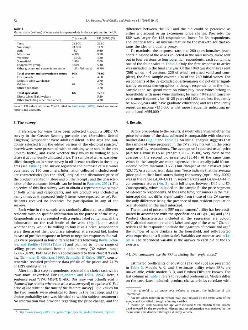
Table 1Market share (volume) of wine sales in supermarkets in the sample and in the UK.

This sample UK (2009) (%)

Tesco 28.80% 26.80Sainsbury’s 21.90% 14.90Asda 18% 9.60Morrisons 4.30% 9.10Waitrose 13.30% 3.80Somerfield 1.90% 2.00Cooperative group 4.60% 5.30Other grocery and convenience stores 1.2% (Aldi only) 6.70%

Total grocery and convenience stores 94% 78.00First quench – 4.60Majestic wine warehouse – 2.70Oddbins 6% 1.00Other specialists – 3.70

Total specialists 6% 12.10Direct wines (Laithwaites) – 5.20Other (including other mail order) – 4.70

Source: UK values are from Mintel, cited in Bainbridge (2009), based on annualreports and accounts.

3 I am grateful to an anonymous referee to suggest the inclusion of thisinformation.

4 Age for wines reporting no vintage year was replaced by the mean value of thesample and identified through a dummy variable.

72 L.A. Panzone / Food Quality and Preference 31 (2014) 69–80

3. The survey

Preferences for wine have been collected though a DBDC CVsurvey in the Greater Reading postcode area (Berkshire, UnitedKingdom). Respondent were adults resident in the area and ran-domly selected from the edited version of the electoral register.2

Interviewees were presented with an existing wine sold in the area(750 ml bottle), and asked whether they would be willing to pur-chase it at a randomly allocated price. The sample of wines was iden-tified through an in-store survey in off-licence retailers in the studyarea (see Table 1). The survey registered the purchase of 260 winespurchased by 160 consumers. Information collected included prod-uct characteristics (on the label), original and discounted price ofthe product (verified in store and on the receipt), and the character-istics of the consumer (details can be found in Panzone, 2012). Theobjective of this first survey was to obtain a representative sampleof both wines and respondents, and any product was included asmany times as it appeared (only 5 items were repeated twice). Par-ticipants received no incentive for participation in any of thesurveys.

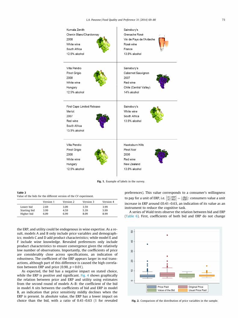
Each wine in the sample was randomly allocated to a differentresident, with no specific information on the purpose of the study.Respondents were presented with a replica label containing all theinformation on the real bottle of the wine (Fig. 1), and askedwhether they would be willing to buy it at a price; respondentswere then asked their purchase intention at a second bid, higherin case of positive response or lower to negative responses. Bid val-ues were prepared in four different formats following Rowe, Schu-lze, and Breffle (1996) (Table 2) and planned to fit the range ofselling prices obtained from a pilot survey (32 wines, range£2.68–£8.99). Bids have been approximated to their closest 9 end-ing (Schindler & Kibarian, 1996; Schindler & Kirby, 1997), consis-tent with revealed preference data (66.0% of the prices and 74.7%of ERPs ending in 9).

After this first step, respondents repeated the choice task with a‘‘was-now’’ advertised ERP (Rajendran and Tellis, 1994). Here, asentence read ‘‘TWO MONTHS AGO, this wine was actually sold in[Name of the retailer where the wine was surveyed] at a price of £ [Fullprice of the wine at the time of the in-store survey]’’. Bid values forthe two rounds were identical to those in the first step, and thechoice probability task was identical (a within-subject treatment).No information was provided regarding the price change, and the

2 http://www.ico.org.uk/for_the_public/topic_specific_guides/electoral_register.

difference between the ERP and the bid could be perceived aseither a discount or an exogenous price change. Precisely, theERP was larger for 123 respondents, lower for 64 respondents,and identical for 7, an unusual feature for the marketplace that re-tains the idea of a quality proxy.

To maximise the response rate, the 260 questionnaires (eachcontaining one of the wines collected in the mall survey) were sentout in four versions to four potential respondents, each containingone of the four scales in Table 2. Only the first response to arrivewas included in the final analysis. Of the 1040 questionnaires sent(260 wines � 4 versions, 226 of which returned valid and com-plete), the final sample covered 194 of the 260 initial wines. Therespondents of the 32 excluded questionnaires did not differ signif-icantly on most demographics, although respondents in the finalsample tend to: spend more on wine; buy more wine; belong tohouseholds with more wine drinkers; be men (10% significance le-vel); more frequently be 18–25 years old (10%) and less frequentlybe 46–55 years old; have graduate education; and less frequentlyreport an income <£15,000 whilst more frequently indicating in-come band >£55,000.3

4. Results

Before proceeding to the results, it worth observing whether theprice behaviour of the data collected is comparable with observedmarket data (Fig. 2 and Table 3). An initial analysis suggests thatthe sample of wine proposed in the CV survey fits within the pricerange used by respondents. The average self-reported usual pricepaid for a wine is £5.41 (range: £3.00–£15.00), very close to theaverage of the second bid presented (£5.44). At the same time,wines in the sample are more expensive than usually paid if con-sidered before discount (£6.79) but cheaper at their market price(£5.17). As a comparison, data from Tesco indicate that the averageprice paid in their local stores during the survey (April–May 2009)was in the range £4.30–£4.11 in supermarkets and £4.46–£4.44 inconvenience stores (Fig. 3), with full prices between £4.5 and £5.Consequently, wines included in the sample fit the price segmentof interest to respondents. At the same time, consumers in the mallintercept did not differ significantly from those of the CV survey,the only difference being the presence of non-resident population(e.g. students) in the mall intercept.

The impact of price and ERP on consumers’ utility has been esti-mated in accordance with the specifications of Eqs. (3a) and (3b).Product characteristics included in the regression are colour,AOC, alcohol content, retailer’s label, and age of the wine.4 Charac-teristics of the respondent include the logarithm of income and age,5

the number of wine drinkers in the household, and self-reportedwine expertise (on a 5-point scale). Variables are summarised in Ta-ble 4. The dependent variable is the answer to each bid of the CVexercise.

4.1. Did consumers use the ERP in stating their preferences?

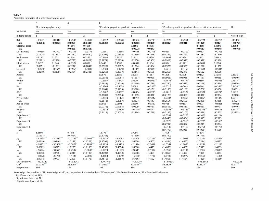
Estimated coefficients of equations (3a) and (3b) are presentedin Table 5. Models A, C, and E estimate utility when ERPs areunavailable, while models B, D, and F when ERPs are known. Thelast column in Table 5 refers to revealed preferences. Models differon the covariates included: product characteristics correlate with

5 Income (in 1000 pounds) and age were included as the median of the incomeband selected by the respondent. Missing income information was replaced by themean value and identified through a dummy variable.

Fig. 1. Example of labels in the survey.

Table 2Value of the bids for the different version of the CV experiment.

Version 1 Version 2 Version 3 Version 4

Lower bid 2.69 3.09 3.59 3.99Starting bid 3.99 4.59 5.39 5.99Higher bid 6.09 6.99 8.09 8.99

010

2030

4050

Price Paid Original PriceValue of the Bid Usual Price Paid

Fig. 2. Comparison of the distribution of price variables in the sample.

L.A. Panzone / Food Quality and Preference 31 (2014) 69–80 73

the ERP, and utility could be endogenous in wine expertise. As a re-sult, models A and B only include price variables and demograph-ics; models C and D add product characteristics; while model E andF include wine knowledge. Revealed preferences only includeproduct characteristics to ensure convergence given the relativelylow number of observations. Importantly, the coefficients of priceare considerably close across specifications, an indication ofrobustness. The coefficient of the ERP appears larger in real trans-actions, although part of this difference is caused the high correla-tion between ERP and price (0.90, p < 0.01).

As expected, the bid has a negative impact on stated choice,while the ERP is positive and significant. Fig. 4 shows graphicallythe relation between price and ERP and utility using estimatesfrom the second round of models A–B: the coefficient of the bidin model A sits between the coefficients of bid and ERP in modelB, an indication that price sensitivity mildly declines when theERP is present. In absolute value, the ERP has a lower impact onchoice than the bid, with a ratio of 0.41–0.63 (1 for revealed

preferences). This value corresponds to a consumer’s willingness

to pay for a unit of ERP, i.e. @U=@ERP@U=@Bid

���

��� ¼ @Bid

@ERP

��

��: consumers value a unit

increase in ERP around £0.41–0.63, an indication of its value as aninstrument to reduce the cognitive task.

A series of Wald tests observe the relation between bid and ERP(Table 6). First, coefficients of both bid and ERP do not change

Table 3Summary statistics of prices of the wines in the sample.

Last bid proposed Original price Price usually paid Market price

Mean £5.44 £6.79 £5.41 £5.17Median £6.09 £5.99 £5.00 £4.39Range £2.69–£8.99 £2.49–£46.49 £3.00–15 £2.37–£37.19

3

3.5

4

4.5

5

5.5

Price - Extra ERP - Extra Price - Express ERP - Express

Fig. 3. Trend in market price and ERP in Tesco stores by size in the study area, June2008–May 2009. Source: courtesy of Dunnhumby Ltd.

74 L.A. Panzone / Food Quality and Preference 31 (2014) 69–80

significantly across bidding rounds. Also, the estimated impact ofbids does not vary across models (a3 ¼ b3), implying that the totalimpact of price plus ERP on choice is larger than that of price alone(a3 þ a4 > b3). Finally, the ERP is as important as the bid in the firstround of bidding, but becomes significantly less important than thebid in the second round (a3 þ a4 < 0). These results indicate thatERPs adds significant information to consumers, but withoutreducing the importance of price. Consequently, the ERP does notseem to remove the informational content of price, but rather inte-grates it. The low number of observations could be responsible forthese conservative results.

Observing all other variables, the likelihood to purchase de-pends only on alcohol content, colour, and missing vintage year.The presence of the ERP might cause an informational bias (Smithet al., 2006): consumers stop using information on alcohol contentand missing year in the second CV, limiting their attention to the

Table 4Variables included in the estimation of the utility function.

Variable Description

ERP External reference price of the wineBid Value of the second bid offered to the respondent (the pr

Round 1 – No ERPRound 2 – No ERPRound 1 – With ERPRound 2 – With ERP

Alcohol Alcohol content of the wineWhite Dummy equal to one if the wine is white (baseline: rosé)Red Dummy equal to one if the wine is red (baseline: rosé)Private label Dummy equal to one if the wine is branded using the retAge of wine Age of the wine (years)No year Dummy equal to one if the wine does not report the vintAOC Dummy equal to one if the wine has an AOC (or equivaleAge Age of the person answering the surveyIncome Yearly household incomeNo income Dummy equal to 1 if the respondent did not report incomHh drinkers Number of wine drinkers in the householdKnowledge Self-reported knowledge, chosen amongst the following o

‘‘No knowledge at all’’‘‘Low knowledge’’‘‘Fairly good knowledge’’‘‘Very good knowledge’’‘‘Wine expert’’

colour of the wine. Changes in the coefficient of specific attributesare consistent with the interference of ERPs on hedonic taste per-ception (Plassmann, O’Doherty, Shiv, & Rangel, 2008), but couldbe partly due to collinearity between ERP and product characteris-tics. Coefficients of product attributes differ substantially in sizeand sign between revealed and stated preference, with alcoholbeing the only coefficient comparable in magnitude and sign acrosspreference type. The different structure imposed by each modelplays a major role in the different results. Apart from age and in-come, demographics contribute modestly to the model, while a sig-nificant q indicates unobservable tastes contained in the residualshave an important role.

To add consistency with existing research on reference pricing(Kalyanaram & Winer, 1995; Kopalle & Lindsey-Mullikin, 2003; Ku-mar, Hurley, Karande, & Reinartz, 1998; Mayhew & Winer, 1992;Mazumdar et al., 2005), the same model is estimated as asymmet-ric reference price model (Mazumdar & Papatla, 2000; Rajendranand Tellis, 1994; Mazumdar et al., 2005) to allow for a different re-sponse to ERP depending on whether it is larger or smaller thanprice. This model incorporates an Internal Reference Value (IRV)equal to the fitted utility from the first CV survey (models A, C,E). In fact, respondents could determine whether to make a pur-chase on the basis of their own inference (Lowe & Alpert, 2010),and the IRV could be the real driver of the previous results. To thisend, the estimated equation is

Uij ¼ uo þu1 � Pi þu2 � IRVij þu3 � Hj � ðERPi � BidiÞþu4 � Lj � ðERPi � BidiÞ þ uij ð8Þ

where H and L are functions equal to one only if the ERP is higher(H) or lower (L) than price.

Results (Table 7) confirm that ERPs influence choice probabilityprimarily when larger than price, while IRVs tend to have a nega-tive impact on choice when the ERP is known (the coefficient is not

Min Max Mean

£2.49 £46.49 £6.79ice to be paid)

3.59 5.99 4.972.69 8.99 5.503.59 5.99 4.992.69 8.99 5.449 14.9 12.810 1 0.370 1 0.55

ailer’s name 0 1 0.141 8 2.44

age year 0 1 0.18nt) denomination 0 1 0.25

3.06 4.17 3.822.01 4.09 3.60

e 0 1 0.081 7 2.03

ptions:0 1 0.130 1 0.580 1 0.230 1 0.060 1 0.00

Table 5Parameter estimation of a utility function for wine.

A B C D E F

SP – demographics only SP – demographics + product characteristics SP – demographics + product characteristics + experience RP

With ERP No Yes No Yes No Yes

Bidding round 1 2 1 2 1 2 1 2 1 2 1 2 Nested logit

Bid �0.3643*** �0.2817*** �0.2534*** �0.2883*** �0.3652*** �0.2928*** �0.2632*** �0.2733*** �0.3922*** �0.2961*** �0.2721*** �0.2759*** �0.3352***

S.E. (0.0754) (0.0282) (0.0961) (0.0431) (0.0828) (0.0325) (0.0988) (0.0459) (0.0832) (0.0316) (0.1029) (0.0471) (�0.0754)Original price 0.1584*** 0.1679*** 0.1166** 0.1735*** 0.1108** 0.1696*** 0.3380***

S.E. (0.0465) (0.0358) (0.0522) (0.0443) (0.0513) (0.0448) (�0.0770)Ln (income) �0.0258 �0.2547** �0.0386 �0.2176 �0.0181 �0.2865** �0.0158 �0.2705* 0.0421 �0.2310* 0.0312 �0.2329

S.E. (0.1224) (0.1291) (0.1432) (0.1450) (0.1296) (0.1354) (0.1460) (0.1479) (0.1289) (0.1341) (0.1481) (0.1510)No income �0.1761 0.1631 0.2056 0.3190 �0.1199 0.3020 0.1711 0.3829 �0.1058 0.3828 0.2362 0.4463

S.E. (0.2891) (0.2838) (0.2773) (0.2822) (0.2874) (0.2850) (0.2950) (0.2901) (0.2918) (0.2913) (0.2978) (0.2998)Hh drinkers 0.0477 0.1346 �0.0374 0.0876 0.0445 0.1587 �0.0318 0.1134 0.0984 0.1911* �0.0051 0.1376

S.E. (0.0951) (0.1081) (0.1232) (0.1047) (0.0928) (0.0997) (0.1204) (0.1064) (0.0925) (0.0995) (0.1226) (0.1052)Ln (age) �0.2540 �0.3545 �0.4955** �0.6089** �0.2969 �0.3750 �0.4841** �0.5823** �0.2215 �0.3450 �0.4681* �0.5819**

S.E. (0.2219) (0.2269) (0.2394) (0.2381) (0.2260) (0.2337) (0.2444) (0.2506) (0.2263) (0.2376) (0.2522) (0.2506)Alcohol 0.0876 0.1989** 0.0293 0.1117 0.1295 0.2198** 0.0462 0.1218 0.2836***

S.E. (0.0955) (0.0981) (0.1157) (0.0960) (0.0963) (0.0988) (0.1151) (0.0985) (0.0840)White �0.4650* �0.4778* 0.0529 �0.5917** �0.4878* �0.4777* 0.0480 �0.5935** 0.5313***

S.E. (0.2688) (0.2710) (0.3119) (0.2730) (0.2760) (0.2675) (0.3169) (0.2694) (0.0759)Red �0.3265 �0.5079 0.0685 �0.5565* �0.3713 �0.5014 0.0614 �0.5535* 0.5434***

S.E. (0.3104) (0.3159) (0.3618) (0.3151) (0.3180) (0.3163) (0.3706) (0.3158) (0.0901)AOC �0.2482 �0.0517 �0.0454 �0.2273 �0.2010 �0.0524 �0.0371 �0.2275 0.1412

S.E. (0.2101) (0.2036) (0.1999) (0.2030) (0.2128) (0.2069) (0.2030) (0.2064) (0.2118)Private label �0.2870 �0.1173 �0.0785 �0.1242 �0.2784 �0.1265 �0.0854 �0.1347 1.6241***

S.E. (0.2613) (0.2557) (0.2877) (0.3147) (0.2664) (0.2560) (0.2880) (0.3118) (0.3577)Age of wine 0.0866 0.0502 0.0300 �0.0317 0.0785 0.0487 0.0373 �0.0235 �0.0088

S.E. (0.0776) (0.0788) (0.0629) (0.0711) (0.0815) (0.0831) (0.0651) (0.0771) (0.0746)No year �0.5574*** �0.5126** �0.5140** 0.0024 �0.5551** �0.5126** �0.5378** �0.0148 1.2417***

S.E. (0.2113) (0.2053) (0.2494) (0.2720) (0.2196) (0.2102) (0.2476) (0.2755) (0.3763)Experience 2 �0.3282 �0.3276 �0.1406 �0.1244

S.E. (0.2446) (0.2404) (0.2915) (0.2915)Experience 3 �0.3976 �0.5215* �0.3725 �0.3565

S.E. (0.2787) (0.2892) (0.3219) (0.3264)Experience 4 �0.9140* �0.4413 �0.2751 �0.1769

S.E. (0.4772) (0.3938) (0.4980) (0.4586)q 1.1895*** 0.7645*** 1.1373*** 0.7256*** 1.1608*** 0.7204***

(0.1637) (0.1614) (0.1748) (0.1690) (0.1760) (0.1740)l1 �3.3235*** �3.7013*** �2.7783** �3.5603*** �2.7139* �1.8083 �2.5808 �2.7211* �2.0663 �1.5088 �2.3294 �2.5854*

S.E. (1.0919) (1.0846) (1.2189) (1.1223) (1.4794) (1.4091) (1.6600) (1.4505) (1.4834) (1.4495) (1.7214) (1.4992)l2 �2.8231*** �3.2309*** �2.3878* �3.1099*** �2.1858 �1.3125 �2.1824 �2.2499 �1.5341 �1.0066 �1.9281 �2.1122

S.E. (1.0902) (1.0717) (1.2235) (1.1199) (1.4790) (1.4074) (1.6680) (1.4473) (1.4859) (1.4465) (1.7315) (1.4969)l3 �2.6944** �3.0571*** �2.2597* �3.0042*** �2.0473 �1.1279 �2.0511 �2.1392 �1.3960 �0.8194 �1.7962 �2.0009

S.E. (1.0918) (1.0705) (1.2241) (1.1193) (1.4792) (1.4072) (1.6698) (1.4461) (1.4863) (1.4453) (1.7335) (1.4953)l4 �1.8878* �2.3758** �1.4425 �2.3809** �1.1884 �0.4049 �1.2160 �1.4780 �0.5406 �0.0977 �0.9568 �1.3355

S.E. (1.0914) (1.0703) (1.2290) (1.1178) (1.4815) (1.4187) (1.6786) (1.4552) (1.4868) (1.4554) (1.7420) (1.5080)Log likelihood �532.6229 �514.4241 �520.3779 �506.4257 �516.0834 �505.2144 �779.0324Chi2 25.7376*** 23.6095*** 51.5653*** 37.7547*** 58.2829*** 40.8127*** 43.51***

Respondents 194 194 194 194 194 194 260

Knowledge: the baseline is ‘‘No knowledge at all’’; no respondent indicated to be a ‘‘Wine expert’’. SP = Stated Preferences; RP = Revealed Preferences.* Significance levels at 10%** Significance levels at 5%*** Significance levels at 1%.

L.A.Panzone

/FoodQ

ualityand

Preference31

(2014)69–

8075

Util

ity

Price

ERP (model B)

Bid(model A)

Bid (model B)

Fig. 4. Graphical representation of the impact of price and ERP on utility.

Table 6Wald tests of equality of coefficients.

H0 A

Bid (round 1) = Bid (round 2) a3, b3 = k 1.56ERP (round 1) = ERP (round 2) a4 = kBid + ERP (round 1) = 0 a3 + a4 = 0Bid + ERP (round 2) = 0Bid + ERP B/D/F (round 1) = Bid A/C/E (round 1) a3 + a4 = b3

Bid + ERP B/D/F (round 2) = Bid A/C/E (round 2)Bid B/D/F (round 1) = Bid A/C/E (round 1) a3 = b3

Bid B/D/F (round 2) = Bid A/C/E (round 2)

All tests have one degree of freedom.* Significance levels at 10%** Significance levels at 5%*** Significance levels at 1%.

Table 7Relative importance of the ERP and IRP in the choice of wine.

A–B C–DDemographics only Demographics + product

Bidding round 1 2 1 2

Bid �0.2505 �0.2944*** �0.0702 �S.E. (0.3530) (0.0472) (0.1593) (

IRV 0.0595 �0.5393*** 0.5605 �S.E. (0.9490) (0.1541) (0.3544) (

ERP (>Bid) 0.0295 0.1016*** 0.0289 0S.E. (0.0257) (0.0360) (0.0248) (

ERP (<Bid) �0.1137* 0.0235 �0.1136 0S.E. (0.0598) (0.0785) (0.0730) (

Average price paid 0.0719 0.0194 0.0667 0S.E. (0.0657) (0.0817) (0.0647) (

q 0.7228*** �0.2944*** 0.5821*** �S.E. (0.1568) (0.0472) (0.2182) (

l1 �1.2628** �0.7337 �0.7891 �S.E. (0.5955) (0.4524) (0.6890) (

l2 �0.9002 �0.2761 �0.4133 �S.E. (0.5926) (0.4523) (0.6885) (

l3 �0.7805 �0.1700 �0.2882 �S.E. (0.5921) (0.4536) (0.6906) (

l4 �0.0211 0.4759 0.5097 0S.E. (0.5985) (0.4543) (0.7170) (

Log�likelihood �526.4878 �527.3043Chi2 15.2871*** 15.8535***

N = 194.* Significance levels at 10%** Significance levels at 5%*** Significance levels at 1%.

76 L.A. Panzone / Food Quality and Preference 31 (2014) 69–80

significant in the first round). As expected, the bid retains a signif-icantly negative coefficient, and results appear robust to variablespecification. The negative influence of IRV when ERPs are avail-able is consistent with Plassmann, O’Doherty, Shiv, and Rangel(2008): consumers give high scores to a low-price wine when priceis unknown, and to a high-price wine when price is known, expect-ing a hedonic performance increasing with price.

4.2. Does the ERP complement or substitute quality informationprovided by price?

Results from Table 5 indicate that consumers use both price andERP in their choices. This section explores whether price retains itsrole as quality proxy once the ERP is available. The same questioncan be asked as whether price and ERPs complement or substituteeach other in the provision of information on product quality. AWald test presented in Table 6 failed to reject the null hypothesis

B C D E F

0.17 1.01 0.01 1.74 0.000.06 1.60 1.800.77 1.68 1.957.95*** 3.13* 3.39*

6.21** 3.73* 3.99**

14.27*** 11.70*** 10.81***

1.33 1.06 1.360.02 0.18 0.18

E–Fcharacteristics Demographics + product characteristics + Experience

1 2

0.1799*** �0.1034 �0.1912***

0.0666) (0.1308) (0.0616)0.2915** 0.4831* �0.2693**

0.1391) (0.2652) (0.1361).1263*** 0.0297 0.1274***

0.0396) (0.0252) (0.0382).0688 �0.1034 0.05950.0864) (0.0725) (0.0857).0107 0.0787 0.00970.0852) (0.0651) (0.0854)0.1799*** 0.6318*** �0.1912***

0.0666) (0.2134) (0.0616)1.1175** �0.7549 �1.1579**

0.5069) (0.6641) (0.5086)0.6534 �0.3806 �0.7004

0.5095) (0.6626) (0.5090)0.5470 �0.2569 �0.5959

0.5104) (0.6635) (0.5089).1023 0.5345 0.03860.5147) (0.6853) (0.5119)

�527.172716.8322***

01

23

4Se

cond

cho

ice

- Firs

t rou

nd

0 1 2 3 4

First choice - First round

Fig. 6. Scatter diagram relating the answers to the two CV surveys (2nd biddinground). Note: The dashed triangle includes respondents reporting a higher utility intheir second choice compared to their first choice. The dotted triangle includesrespondents doing the opposite.

Fig. 5. Graphical representation of the impact of full price of the wine on utility atchanging levels of discounts.

Table 8Conditional log-odds ratios of revising utility and the relative position of the ERP.

ERP > Bid ERP < Bid

Revised up 6.4444*** 0.1648***

Revised down 0.1552*** 6.0677***

Adjusted by self-reported knowledge and purchase rate. Observations = 69(respondents who changed in the first choice across survey).

* Significance levels at 10** Significance levels at 10%

*** Significance levels at 1%

6 I am indebted to an anonymous referee for suggesting this point.

L.A. Panzone / Food Quality and Preference 31 (2014) 69–80 77

that the informational component of price remains the same whenthe ERP is known, so that ðdC þ dIÞ ¼ ðdC þ dP

I Þ. This point is sup-ported by a similar coefficient of price in the presence or absenceof ERPs (Table 5). Wald tests also determine that the ERP addsexplanatory power to the model, ðdC þ dP

I Þ þ ðdERPI Þ > ðdC þ dIÞ, and

the overall impact of bid and ERP is negative,ðdC þ dP

I Þ þ ðdERPI Þ < 0. These results imply that ERPs contribute

with new information, i.e. ðdERPI Þ > 0, but consumers keep using

price to infer information on quality. In other words, price doesnot seem to lose its role as quality proxy, and the ERP complementsit. A formal identification of each d requires an experimental set-ting and cannot be done using the present dataset.

4.3. What is the impact of the rate of discount on utility?

Besides communicating information, the ERP informs on thediscount rate p, which can impact price sensitivity. As mentionedabove, market price is a fraction of the original price:Bidi ¼ ð1� piÞ � ERPi, where 0 6 pi 6 1. Using the coefficients ofthe second bidding round of model B (Table 5, similar results areobtained from all other models), utility can be written as

Ui ¼ 0:1679� ERPi � 0:2883� Bidi

¼ 0:1679� ERPi � 0:2883� ½ð1� piÞ � ERPi�

which reduces to

Ui ¼ ½�0:1204þ ð0:2883� piÞ� � ERPi ð9Þ

Eq. (9) indicates that purchase probability is negatively relatedto price (�0.1204) in the absence of a discount (pi = 0). This prob-ability starts rising as discounts grow, reaching positive values fordiscounts larger than 41.76% (Fig. 5). The positive contribution ofdiscounts is caused by a decline in sensitivity to the cost compo-nent of price (as in Eq. (4)): money spent becomes relatively lessimportant when the ERP is available. This result also suggests thatconsumers might increase their attention to the potential moneysaved of price as discounts grow.

More generally, Fig. 5 shows that for sufficiently high discountsthe probability of a purchase increases with the original price, par-ticularly for expensive options with a large discount becauseUðERPi;piÞ > 0, ceteris paribus. This result suggest that in an ex-treme scenario consumers could purchase an item generating neg-ative utility in all other attributes, UðXi;DjÞ < 0, as long as totalutility is positive, i.e. UðERPi;piÞ þ UðXi;DjÞ > 0. This finding indi-cates that ERPs could lead to suboptimal choices that consumersmight fail to realise, i.e. the consumer might purchase somethingshe dislikes just because it is discounted. This cognitive shortcutcould conflict with policy instruments (alcohol taxes, see Panzone,2012), or stimulate the purchase of unnecessary goods and

increase waste. Indeed, high quality products tend to have highERP (Bagwell & Riordan, 1991) so that UðXi;DjÞ > 0 wheneverUðERPi;piÞ > 0, but future research should assess under which con-dition this relationship holds.

4.4. Did consumers revise their choice when the ERP was available?

The final step of this analysis explores how consumers used theinformation contained in the ERP. In particular, the data indicatesthat ERPs play a positive role in the probability of a purchasethrough several different channels. Firstly, ERPs could reduceuncertainty: in the second bidding round, 18 respondents (out of194) reported to be ‘‘Unsure’’ when the ERP was unavailable (15in the first bidding round), and only 9 when the ERP was supplied(both bidding rounds), with only 3 people reporting uncertainty inboth surveys (2 in the first round). Similarly, consumers might useERPs as anchor for their choices: decisions on whether to purchasean item or not might depend on the relative position of price. Infact, ERPs sets a reference point and prices lower than the ERPmight seem reasonable even if the price is still higher than whatthe wine is really worth. Importantly, part of this decline in uncer-tainty might have been caused by a repeated-choice task, whereconsumers gained knowledge (e.g. Hoeffler & Ariely, 1999) or bya testing effect (e.g., Porath, MacInnis, & Folkes, 2010), rather thanthe presence of an ERP.6

Consequently, it appears possible that ERPs constitute apossible source of adaptive bias: ERPs may be used to maketime-efficient choices, reducing the costs of cognitive errors rather

78 L.A. Panzone / Food Quality and Preference 31 (2014) 69–80

than their number (Haselton & Buss, 2003; Kool, McGuire, Rosen, &Botvinick, 2010). The correct determination of an adaptive biashinges on the knowledge of the real utility the consumer obtainsfrom a good, but it is impossible to establish which CV collectedthe ‘‘real’’ expected utility. On average, the stated utility in thetwo initial bidding rounds (which are strictly comparable) withand without knowledge of the ERP do not differ, going from 1.89(without ERP) to 1.91 (with ERP) (p = 0.90), and are strongly corre-lated (Pearson correlation = 0.75, p < 0.01). Nevertheless, 69 out of194 respondents (36%) revised their initial intention to purchasewhen the ERP was supplied, with 38 (55%) moving upwards and31 (45%) downwards (Fig. 6).

The odds of the probability of revising up or down were esti-mated for those 69 respondents who revised their choices usingthe following logistic regressions:

CUij ¼ kU0 þ kU

1 � KNi þ kU2 � PRij þ kU

3 � Hj þ kU4 � Lj þ eij ð10aÞ

CDij ¼ kD0 þ kD

1 � KNi þ kD2 � PRij þ kD

3 � Hj þ kD4 � Lj þ uij ð10bÞ

where CU and CD indicate a change up or down the utility scale, KNis self-reported knowledge, PR is the purchase rate, while H and Lindicate whether the ERP is higher or lower than the bid, respec-tively. Odd ratios (Table 8) indicate that the probability of a pur-chase increases significantly if ERP is larger than price, while theprobability of rejecting the purchase increases significantly if theERP is lower than price, in both cases of more than 600%. Very infre-quent is an increase in the likelihood of a purchase when ERP < bidor viceversa. Consequently, the presence of ERPs contributes to con-sumer choices by providing a reference against which price isevaluated.

5. Discussion and conclusions

The objective of this work is to understand the impact of ERPson consumer behaviour. In particular, the article explores whetherand to what extent the presence of ERPs influences consumerchoices. Compared to previous research (Kalyanaram & Winer,1995; Kopalle & Lindsey-Mullikin, 2003; Kumar et al., 1998; May-hew & Winer, 1992), the aim is to understand the informationaland priming role of ERPs, and in this respect the paper is novel. Thisarticle uses a stated preference approach (opposite to the generaluse of revealed preferences) to remove the correlation betweenERP and prices. Through a CV survey, consumers reported theirintention to purchase the same wine at a random bid twice, onceignoring and once knowing the full price of the wine some time be-fore the survey (a ‘‘Was-now’’ advertised ERP). The survey exploredpreferences for wine in the Greater Reading area (UK), using a rep-resentative sample of wines sold in supermarkets of the samestudy area. The small sample size and the narrow range of consum-ers in the survey from a geographical point of view substantiallylimit the generalisability of the findings of this article, but identifysignificant patterns of behaviour in a homogeneous market.

The overall picture drawn by the results section is an ‘‘ERP dom-inance’’: the presence of both ERP and price directs choices to-wards discounted expensive products. In fact, consumers: (a) relyimportantly on price and ERP in their choices; and (b) anchor theirexpectations to the ERP by evaluating price relative to this infor-mation. As a result, ERPs lead consumers to buy primarily on fulland discounted prices, paying less attention to other observablequality signals. In the extreme case where the utility for priceand discounts is sufficiently high, consumers could even chooseproducts with low or negative utility from other characteristics.This behaviour is indicative of adaptive reasoning: consumersaim at reducing the cognitive costs of errors rather than their num-ber when faced with risky decisions (Hilbert, 2012; Kool et al.,

2010). Consumers can then reduce search costs for informationby relying on high ERPs, willingly accepting the probability of mis-take (Haselton & Buss, 2003; Kool et al., 2010). These results arerelevant also in the use of price instruments in public policy, astaxation interacts with ERPs (see Panzone, 2012).

Four sets of results provide a picture that contributes to theunderstanding of how consumers use ERPs in their choices. Firstly,ERPs positively influence the probability of a purchase. Consumersare nudged into preferring high ERPs because they generate expec-tations on the unobservable quality that is imperfectly availablewhen price is alone. Importantly, the ERP anchors consumer pref-erences, leading consumers to evaluate the price to pay with re-spect to the full price of the same good. The impact of priceremains the same when the ERP is present, but ERPs provide anincentive towards a purchase by reducing the weight given to priceas a cost. Additionally, consumers seem to rely less on observablecharacteristics and unobservable preferences when ERPs areprovided.

Second, ERPs nudge consumers towards the purchase of goodswith high full price and low discounted price, possibly leading tooptimistic expectations over unobservable quality. In fact, ERPsprovide useful information regarding the quality of the marketedgood that complements the internal valuation of consumers. Thisfinding is consistent with existing reference price theory accordingto which acceptance of external price information is mediated byinternal quality valuation (e.g. Mazumdar et al., 2005). The ERPalso has an important role on the decision-making process becauseit induces consumers to revise their choice, particularly when theERP is greater than price. This ‘‘ERP dominance’’ is very likely astrategy that aims at reducing the cognitive costs of choices inmarkets with high information loads, where ERP is used as a qual-ity cue. The empirical fieldwork analysed the wine market (a rela-tive luxury) in the mass retail sector (a commodity market), whichis characterised by a large heterogeneity of supply. Results mightbe stronger in markets where prices have a strong informationalcomponent, such as luxury goods.

Third, ERPs seem to complement rather than reduce the infor-mational content of prices. This external stimulus has no signifi-cant impact on the coefficient of the bid: its value is notsignificantly different in the absence or presence of external priceinformation. The surprising result is that in absence of ERPs con-sumers appear optimistic in their price-quality inference, wherethe quality component of price seems not to vary too much oncethe ERP is known. This result is consistent with theories of com-pensatory reasoning (Chernev & Hamilton, 2008): the existenceof a good with undesirable features (such as price) can be justifiedonly on the grounds of desirable unobservable quality. Conse-quently, consumers might use ERPs to confirm the earlier qualityinference. At the same time, adaptation theory (Lee, Loewenstein,Ariely, Hong, & Young, 2008) indicates consumers may adapt byaccepting the quality of existing options, viewing available optionsoptimistically.

Finally, the ERP operates through a reduction in the relevance ofprice as a cost. As discounts increase, the relative importance ofprice as quality proxy increases, and the utility of price can becomepositive for high discounts. Hence, consumers can be nudged into apurchase by providing both full and discounted price. In an ex-treme case, consumers could purchase a good expecting negativeutility from observable product characteristic and positive utilityfrom price and discount. It is unclear whether consumersconsciously prefer products that happen to be on discount andpatiently wait for a lower price to purchase them; or subcon-sciously direct their attention to price rather than product charac-teristics in the presence of a discount. Answers to debriefingquestions suggest consumers are often aware that knowledge ofthe ERP changed their answer. However, it is unclear whether all

L.A. Panzone / Food Quality and Preference 31 (2014) 69–80 79

consumers are aware of this mechanism (Plassmann et al., 2008,suggests otherwise) and if they estimate correctly the magnitudeof the impact.

Before concluding, it is worth mentioning the caveats of thepresent work. The first important limitation is presenting two sur-veys consecutively within the same questionnaire. Apart fromlearning (e.g. Hoeffler & Ariely, 1999) and testing effects (e.g., Por-ath et al., 2010), respondents could have seen the ERP beforeanswering the first task, leading to similar coefficients for thebid. Different estimates for other attributes suggest this problemwas not fundamental. Equally, two surveys within the same ques-tionnaire might induce consumers to reflect on their willingness tobe consistent in their response, despite the questionnaire indicat-ing that the second task was intended as a completely new pur-chase (as in Bateman, Burgess, Hutchinson, & Matthews, 2008). Aconsistency bias should underestimate the number of consumersrevising choices, therefore providing a possible downward biasthat reinforces the findings of this article. At the same time, the dif-ferent coefficients for attributes in the two exercises suggest thatconsistency did not undermine the implications of this article.

A second caveat is methodological. The survey manipulated thepresence of ERP in a within-subject setting by always providing achoice task without an ERP first and then a choice task with anERP (no filler task between them). Accordingly, part of the resultsmight be a consequence of an ordering bias (Halvorsen, 1996) thatwould give an upward bias to the effects of the ERP. However,ordering bias tends to underestimate coefficients in the secondtask, partially compensating the bias from the design, and overes-timate coefficients in the first task, possibly providing optimisticestimates when ERPs were not available. Furthermore, consumersreact differently to different type of promotions (DelVecchio,2005): this analysis only focuses on absolute monetary savings,and results might not be transferable to non-price promotions ordifferent framing (e.g. percentages).

To conclude, results in this article provide useful insights on theability of the ERP to facilitate choices. Further research should ex-plore the generalisability of these results, as well as giving a betterinsight on the implications of the reliance on the ERP as a proxy ofquality can have on consumers’ choices, welfare, and informationexternalities.

Acknowledgements

I am thankful to Lorenza Quintaliani, Giacomo Zanello, VivianaAlbani, Ariane Kehlbacher, Noppamas Karoon, Elisabetta Pirodda,and Aurelia Samuel for their support in the data collection process.I am indebted to Richard Tiffin, Kelvin Balcombe, and Lucia Baldifor their extremely valuable inputs and support in the econometricanalysis. I am also grateful to: Ada Wossink, Garth Holloway, BruceTraill, and Iain Fraser for useful conversations; seminar partici-pants at the University of Milan and participants to the AAWE con-ference in Bolzano for their valuable insights on a previous versionof the paper; Carlo Reggiani, and Denton Marks for useful sugges-tions and encouraging comments. The author is the sole responsi-ble of the remaining errors.

Appendix A. Supplementary data

Supplementary data associated with this article can be found, inthe online version, at http://dx.doi.org/10.1016/j.foodqual.2013.08.003.

References

Akerlof, G. A. (1970). The market for ‘‘lemons’’: Quality uncertainty and the marketmechanism. The Quarterly Journal of Economics, 84(3), 488–500.

Alba, J. W., & Hutchinson, J. W. (2000). Knowledge calibration: What consumersknow and what they think they know. Journal of Consumer Research, 27(2),123–156.

Alberini, A., Boyle, K., & Welsh, M. (2003). Analysis of contingent valuation datawith multiple bids and response options allowing respondents to expressuncertainty. Journal of Environmental Economics and Management, 45(1), 40–62.

Ariely, D., Loewenstein, G., & Prelec, D. (2003). ‘‘Coherent arbitrariness’’: Stabledemand curves without stable preferences. The Quarterly Journal of Economics,118(1), 73–106.

Ariely, D., & Norton, M. I. (2011). From thinking too little to thinking too much: Acontinuum of decision making. Wiley Interdisciplinary Reviews: Cognitive Science,2(1), 39–46.

Bagwell, K., & Riordan, M. H. (1991). High and Declining Prices Signal ProductQuality. The American Economic Review, 81(1), 224–239.

Bainbridge, J. (2009). The future looks rosé. Marketing, 19, 26–27.Basmann, R. L., Molina, D. J., & Slottje, D. J. (1988). A note on measuring Veblen’s

theory of conspicuous consumption. The Review of Economics and Statistics,70(3), 531–535.

Bateman, I. J., Burgess, D., Hutchinson, W. G., & Matthews, D. I. (2008). Learningdesign contingent valuation (LDCV): NOAA guidelines, preference learning andcoherent arbitrariness. Journal of Environmental Economics and Management,55(2), 127–141.

Broniarczyk, S. M., & Alba, J. W. (1994). The role of consumers’ intuitions ininference making. Journal of Consumer Research, 21(3), 393–407.

Cameron, T. A., & Quiggin, J. (1994). Estimation using contingent valuation datafrom a ‘‘dichotomous choice with follow-up’’ questionnaire. Journal ofEnvironmental Economics and Management, 27(3), 218–234.

Carson, R. T. (2000). Contingent Valuation: A user’s guide. Environmental Science andTechnology, 34(8), 1413–1418.

Carson, R. T., Flores, N. E., & Meade, N. F. (2001). Contingent valuation: Controversiesand evidence. Environmental and Resource Economics, 19(2), 173–210.

Chaney, I. M. (2000). External search effort for wine. International Journal of WineMarketing, 12(2), 5–21.

Chen, C. Y. (2009). Who I am and how I think: The impact of self-construal on theroles of internal and external reference prices in price evaluations. Journal ofConsumer Psychology, 19(3), 416–426.

Cheng, L. L., & Monroe, K. B. (2013). An appraisal of behavioral price research (part1): Price as a physical stimulus. AMS Review, 1–27. http://link.springer.com/article/10.1007%2Fs13162-013-0041-1.

Chernev, A., & Hamilton, R. (2008). Compensatory reasoning in choice. In ArieKruglanski & Joseph Forgas (Eds.), The social psychology of consumer behavior,frontiers of social psychology. New York (NY): Taylor & Francis Group.

Cooper, R., & Ross, T. W. (1984). Prices, product qualities and asymmetricinformation: The competitive case. The Review of Economic Studies, 51(2),197–207.

Cummings, R. G., & Taylor, L. O. (1999). Unbiased value estimates for environmentalgoods: Cheap talk design for the contingent valuation method. The AmericanEconomic Review, 89(3), 649–665.

Dawson, J. (2013). Retailer activity in shaping food choice. Food Quality andPreference, 28(1), 339–347.

DelVecchio, D. (2005). Deal-prone consumers’ response to promotion: The effects ofrelative and absolute promotion value. Psychology and Marketing, 22(5),373–391.

Dhar, R., & Novemsky, N. (2008). Beyond rationality: The content of preferences.Journal of Consumer Psychology, 18(3), 175–178.

Ding, M., Ross, W. T., Jr., & Rao, V. R. (2010). Price as an indicator of quality:Implications for utility and demand functions. Journal of Retailing, 86(1), 69–84.

Drummond, G., & Rule, G. (2005). Consumer confusion in the UK wine industry.Journal of Wine Research, 16(1), 55–64.

Gerstner, Eiten. (1985). Do Higher Prices Signal Higher Quality? Journal of MarketingResearch, 22(2), 209–215.

Greene, William H., Hensher, David A. (2009). Modeling ordered choices. Availablefrom <http://pages.stern.nyu.edu/~wgreene/DiscreteChoice/Readings/OrderedChoiceSurvey.pdf>.

Halvorsen, Bente (1996). Ordering effects in contingent valuation surveys.Environmental and Resource Economics, 8(4), 485–499.

Hanemann, W. M. (1984). Welfare evaluations in contingent valuation experimentswith discrete responses. American Journal of Agricultural Economics, 66(3),332–341.

Haselton, M. G., & Buss, D. M. (2003). Biases in social judgment: Design flaws ordesign features? In J. Forgas, K. Williams, & B. von Hippel (Eds.), Responding tothe social world: Implicit and explicit processes in social judgments and decisions.New York, NY: Cambridge.

Hilbert, M. (2012). Toward a synthesis of cognitive biases: How noisy informationprocessing can bias human decision making. Psychological Bulletin, 138(2),211–237.

Hoeffler, S., & Ariely, D. (1999). Constructing stable preferences: A look intodimensions of experience and their impact on preference stability. Journal ofConsumer Psychology, 8(2), 113–139.

Hsee, C. K., & Zhang, J. (2004). Distinction bias: Misprediction and mischoice due tojoint evaluation. Journal of Personality and Social Psychology, 86(5), 680–695.

Islam, T., Louviere, J. J., & Burke, P. F. (2007). Modeling the effects of including/excluding attributes in choice experiments on systematic and randomcomponents. International Journal of Research in Marketing, 24(4), 289–300.

Jaeger, S. R. (2006). Non-sensory factors in sensory science research. Food Qualityand Preference, 17(1–2), 132–144.

80 L.A. Panzone / Food Quality and Preference 31 (2014) 69–80

Kalyanaram, G., & Winer, R. S. (1995). Empirical generalizations from referenceprice research. Marketing Science, 14(3), G161–G169.

Kirmani, A., & Rao, A. R. (2000). No pain, no gain: A critical review of the literatureon signaling unobservable product quality. Journal of Marketing, 64(2), 66–79.

Kool, W., McGuire, J. T., Rosen, Z. B., & Botvinick, Matthew M. (2010). Decisionmaking and the avoidance of cognitive demand. Journal of ExperimentalPsychology: General, 139(4), 665–682.

Kopalle, P. K., Kannan, P. K., Boldt, L. B., & Arora, N. (2012). The impact of householdlevel heterogeneity in reference price effects on optimal retailer pricing policies.Journal of Retailing, 88(1), 102–114.

Kopalle, P. K., & Lindsey-Mullikin, J. (2003). The impact of external reference priceon consumer price expectations. Journal of Retailing, 79(4), 225–236.

Kopalle, P. K., Mela, C. F., & Marsh, L. (1999). The dynamic effect of discounting onsales: Empirical analysis and normative pricing implications. Marketing Science,18(3), 317–332.

Kumar, V., Hurley, M., Karande, K., & Reinartz, W. J. (1998). The impact of internaland external reference prices on brand choice: The moderating role ofcontextual variables. Journal of Retailing, 74(3), 401–426.

Lee, L., Loewenstein, G., Ariely, D., Hong, J., & Young, J. (2008). If i am not hot, are youhot or not?: Physical-attractiveness evaluations and dating preferences as afunction of one’s own attractiveness. Psychological Science, 19, 669–677.

Leibenstein, H. (1950). Bandwagon, Snob, and Veblen effects in the theory ofconsumers’ demand. The Quarterly Journal of Economics, 64(2), 183–207.

Lockshin, L., Jarvis, W., d’Hauteville, F., & Perrouty, J.-P. (2006). Using simulationsfrom discrete choice experiments to measure consumer sensitivity to brand,region, price, and awards in wine choice. Food Quality and Preference, 17(3–4),166–178.

Lowe, B., & Alpert, F. (2010). Pricing strategy and the formation and evolution ofreference price perceptions in new product categories. Psychology andMarketing, 27(9), 846–873.

Lusk, J. L. (2003). Effects of cheap talk on consumer willingness-to-pay for goldenrice. American Journal of Agricultural Economics, 85(4), 840–856.

Mayhew, G. E., & Winer, R. S. (1992). An empirical analysis of Internal and ExternalReference Prices using scanner data. The Journal of Consumer Research, 19(1),62–70.

Mazumdar, T., & Papatla, P. (2000). An investigation of reference price segments.Journal of Marketing Research, 37(2), 246–258.

Mazumdar, T., Raj, S. P., & Sinha, I. (2005). Reference price research: Review andpropositions. Journal of Marketing, 69, 84–102.

Milgrom, P., & Roberts, J. (1986). Price and advertising signals of product quality.Journal of Political Economy, 94(4), 796–821.

Mitchell, V. W., & Greatorex, M. (1989). Risk reducing strategies used in the purchaseof wine in the UK. International Journal of Wine Business Research, 1(2), 31–46.

Monroe, K. B. (1973). Buyers’ subjective perceptions of price. Journal of MarketingResearch, 10(1), 70–80.

Mueller, S., Lockshin, L., & Louviere, J. (2010). What you see may not be what youget: Asking consumers what matters may not reflect what they choose.Marketing Letters, 21(4), 335–350.

Palazon, M., & Delgado-Ballester, E. (2009). Effectiveness of price discounts andpremium promotions. Psychology and Marketing, 26(12), 1108–1129.

Panzone, L. (2012). Alcohol tax, price–quality proxy and discounting: A reason whyalcohol taxes may rebound. Journal of Agricultural Economics, 63(3).

Park, J. H., & MacLachlan, D. L. (2008). Estimating willingness to pay withexaggeration bias-corrected contingent valuation method. Marketing Science,27, 691–698.

Peri, Claudio. (2006). The universe of food quality. Food Quality and Preference, 17(1–2), 3–8.

Plassmann, H., O’Doherty, J., Shiv, B., & Rangel, A. (2008). Marketing actions canmodulate neural representations of experienced pleasantness. Proceedings of theNational Academy of Sciences (PNAS), 105, 1050–1054.

Porath, C., MacInnis, D., & Folkes, V. (2010). Witnessing Incivility among employees:Effects on consumer anger and negative inferences about companies. Journal ofConsumer Research, 37(2), 292–303.

Rajendran, K. N., & Tellis, Gerard. J. (1994). Contextual and Temporal Components ofReference Price. Journal of Marketing, 58(1), 22–34.

Rao, A. (2005). The quality of price as a quality cue. Journal of Marketing Research,42(4), 401–405.

Rao, A. R., & Monroe, K. B. (1989). The effect of price, brand name, and store name onbuyers’ perceptions of product quality: An integrative review. Journal ofMarketing Research, 26(3), 351–357.

Ritchie, C. (2007). Beyond drinking: The role of wine in the life of the UK consumer.International Journal of Consumer Studies, 31(5), 534–540.

Rowe, R. D., Schulze, W. D., & Breffle, W. S. (1996). A test for payment card biases.Journal of Environmental Economics and Management, 31(2), 178–185.

Scarpa, R., Gilbride, T. J., Campbell, D., & Hensher, D. A. (2009). Modelling attributenon-attendance in choice experiments for rural landscape valuation. EuropeanReview of Agricultural Economics, 36(2), 151–174.

Schindler, R. M., & Kibarian, T. M. (1996). Increased consumer sales responsethrough use of 99-ending prices. Journal of Retailing, 72(2), 187–199.

Schindler, R. M., & Kirby, P. N. (1997). Patterns of rightmost digits used in advertisedprices: Implications for nine ending effects. Journal of Consumer Research, 24(2),192–201.

Shiv, B., Carmon, Z., & Ariely, D. (2005). Placebo effects of marketing actions:Consumers may get what they pay for. Journal of Marketing Research, 42,383–393.

Smith, N. K., Larsen, J. T., Chartrand, T. L., Cacioppo, J. T., Katafiasz, H. A., & Moran, K.E. (2006). Being bad is not always good: Affective context moderates theattention bias toward negative information. Journal of Personality and SocialPsychology, 90(2), 210–220.

Spence, M. (1973). Job market signaling. The Quarterly Journal of Economics, 87(3),355–374.

Spence, M. (2002). Signaling in retrospect and the informational structure ofmarkets. The American Economic Review, 92(3), 434–459.

Stiglitz, J. E. (1987). The causes and consequences of the dependence of quality onprice. Journal of Economic Literature, 25(1), 1–48.

Thomas, M. (2013). Commentary on behavioral price research: the role of subjectiveexperiences in price cognition. AMS Review, 1–5. http://link.springer.com/article/10.1007%2Fs13162-013-0044-y.

Tversky, A., & Kahneman, D. (1974). Judgment under uncertainty: Heuristics andbiases. Science, 185, 1124–1130.

Urbany, Joel. E., Bearden, William. O., & Weilbaker, Dan. C. (1988). The Effect ofPlausible and Exaggerated Reference Prices on Consumer Perceptions and PriceSearch. Journal of Consumer Research, 15(1), 95–110.

Veblen, T. (1998). The theory of the leisure class. Amherst, NY: Prometheus Books[Originally published in 1899].

Venkatachalam, L. (2004). The contingent valuation method: A review.Environmental Impact Assessment Review, 24(1), 89–124.

Wang, H. (1997). Treatment of ‘don’t-know’ responses in contingent valuationsurveys: A random valuation model. Journal of Environmental Economics andManagement, 32(2), 219–232.

Welsh, M. P., & Poe, G. L. (1998). Elicitation effects in contingent valuation:Comparisons to a multiple bounded discrete choice approach. Journal ofEnvironmental Economics and Management, 36(2), 170–185.

Wertenbroch, K., & Skiera, B. (2002). Measuring consumers’ Willingness to pay atthe point of purchase. Journal of Marketing Research, 39(2), 228–241.

Zeithaml, V. A. (1988). Consumer perceptions of price, quality, and value: Ameans-end model and synthesis of evidence. The Journal of Marketing, 52(3),2–22.