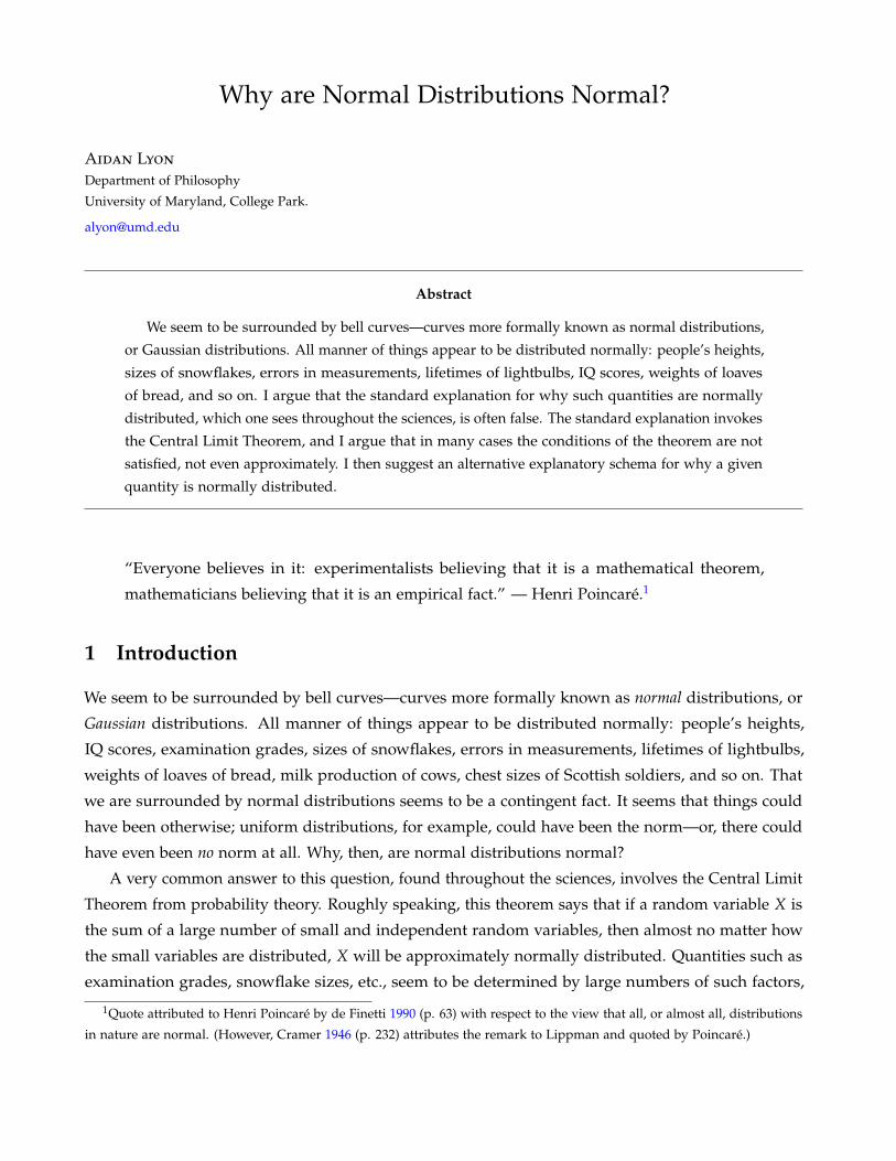
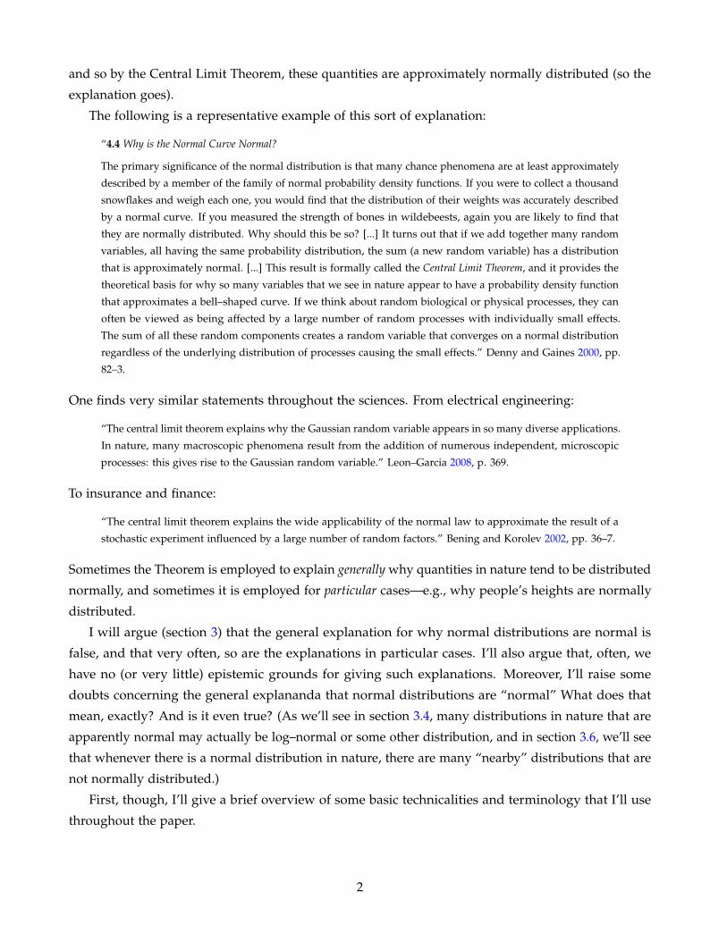
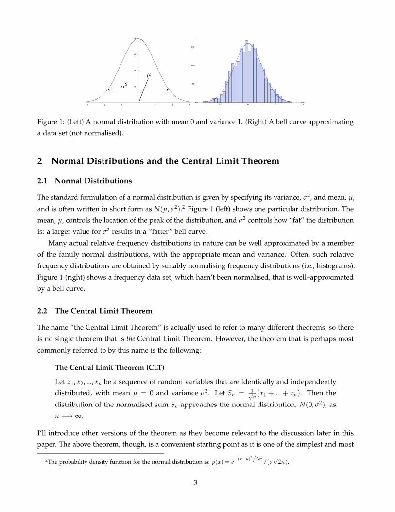
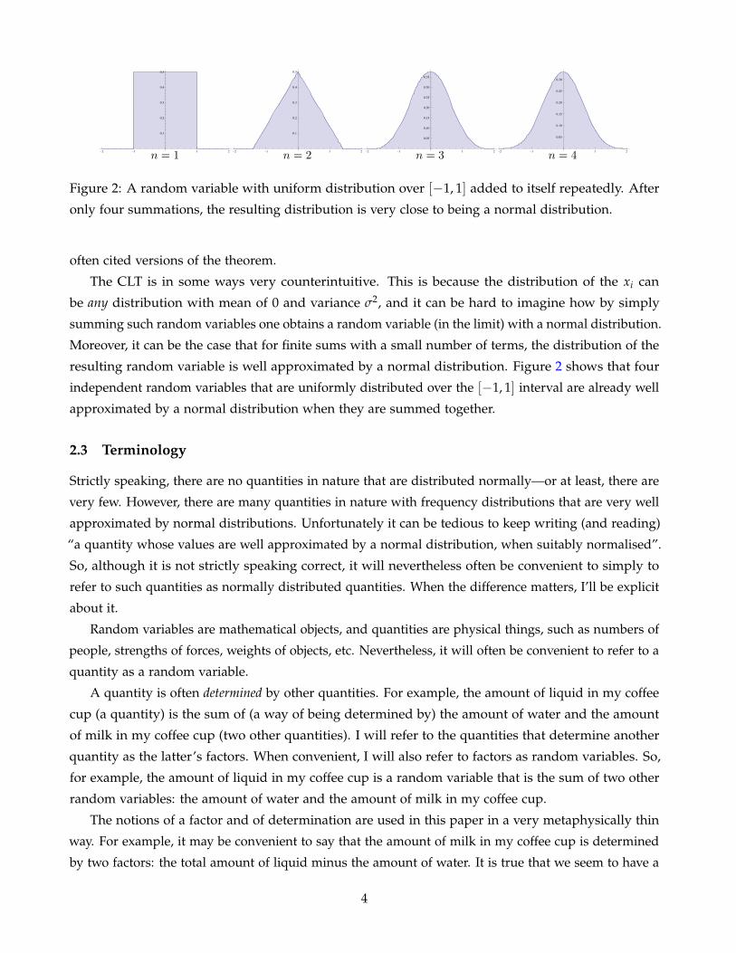
Why are Normal Distributions Normal? Aidan Lyon Department of Philosophy University of Maryland, College Park. [email protected]Abstract We seem to be surrounded by bell curves—curves more formally known as normal distributions, or Gaussian distributions. All manner of things appear to be distributed normally: people’s heights, sizes of snowflakes, errors in measurements, lifetimes of lightbulbs, IQ scores, weights of loaves of bread, and so on. I argue that the standard explanation for why such quantities are normally distributed, which one sees throughout the sciences, is often false. The standard explanation invokes the Central Limit Theorem, and I argue that in many cases the conditions of the theorem are not satisfied, not even approximately. I then suggest an alternative explanatory schema for why a given quantity is normally distributed. “Everyone believes in it: experimentalists believing that it is a mathematical theorem, mathematicians believing that it is an empirical fact.” — Henri Poincar´ e. 1 1 Introduction We seem to be surrounded by bell curves—curves more formally known as normal distributions, or Gaussian distributions. All manner of things appear to be distributed normally: people’s heights, IQ scores, examination grades, sizes of snowflakes, errors in measurements, lifetimes of lightbulbs, weights of loaves of bread, milk production of cows, chest sizes of Scottish soldiers, and so on. That we are surrounded by normal distributions seems to be a contingent fact. It seems that things could have been otherwise; uniform distributions, for example, could have been the norm—or, there could have even been no norm at all. Why, then, are normal distributions normal? A very common answer to this question, found throughout the sciences, involves the Central Limit Theorem from probability theory. Roughly speaking, this theorem says that if a random variable X is the sum of a large number of small and independent random variables, then almost no matter how the small variables are distributed, X will be approximately normally distributed. Quantities such as examination grades, snowflake sizes, etc., seem to be determined by large numbers of such factors, 1 Quote attributed to Henri Poincar ´ e by de Finetti 1990 (p. 63) with respect to the view that all, or almost all, distributions in nature are normal. (However, Cramer 1946 (p. 232) attributes the remark to Lippman and quoted by Poincar´ e.)
where ci is the actual mean of the random variable xi. If we can show that W − 1000 is normally
distributed, then we can conclude that W is normally distributed because normal distributions are
invariant under additions of a scalar.4Assuming we don’t use another version of the CLT, which would also be a way of dealing with the difficulty. We will
eventually have to do this anyway, and I discuss how one might use other versions of the CLT later in the paper.
6
3.2 Varying Variances and Probability Densities
It remains to be shown that the xi − ci are identically and independently distributed—for convenience,
I’ll call the new random variables x′i . Let’s first start with the identity of the distributions, which I’ll
call pi. By definition, their means exist and are all 0, but there is more to a distribution than its mean.
For example, there is its variance. Are the variances of each of the x′i all identical? It seems plausible
that in fact they are not. For example, the variance associated with the amount of salt is plausibly
smaller than the variance associated with the amount of flour. If the variances are not all identical,
then the CLT doesn’t apply, and the explanation doesn’t go through. Moreover, for all we know, it’s
possible that some of the pi have different functional forms. For example, the weight of flour used
(minus 625 g) may be a normal distribution, but the amount of water lost during the baking process
(minus its actual mean) might be a symmetric bimodal distribution, with probability mass heaped
over ±1 and almost entirely absent over 0.
Fortunately, there is a more complicated version of the CLT that relaxes the condition that the
distributions be of the same form (or have the same variance)—so long as they satisfy what is called
the Lindeberg condition.
Central Limit Theorem (Lindeberg–Feller): Let xi be mutually independent random vari-
ables with distributions pi such that E(xi) = 0 and Var(xi) = σ2i . Define s2
n = σ21 + ... + σ2
n .
Then, if
(Lindeberg condition) For every t > 0,√
sn
n
∑k=1
∫|y|≥tsn
y2 pi{dy} −→ 0
then the distribution of Sn = (x1 + ... + xn)/sn tends to the normal distribution with mean
of 0 and variance of 1. Feller 1971, p. 262.
The Lindeberg condition is complicated, but it entails a simpler condition that is easier to understand
and is still informative: it guarantees that the individual variances are small compared to their sum
(Feller 1971, p. 262–3).
Are the variances small with respect to their sum? It seems that they need not be. For example,
the variance associated with the weight of flour might be quite large compared with the sum of the
variances. One way for this to happen is if the baker has very precise instruments for measuring water,
sugar, yeast, salt, etc., but a fairly imprecise instrument for measuring flour (e.g., the baker “eye balls”
it). The resulting weights of the breads that the baker produces can be normally distributed in such a
scenario, and yet this latest version of the CLT won’t apply.
One option in response to this is to factor out the random variables with large variances.5 For
example, instead of trying to use the CLT to show that (W − 1000) is normally distributed, one might
try use the CLT to show that:
(W ′ − x′1 − x′2) = x′3 + ... + x′n5This method of factoring out problematic factors is very similar to Galton’s 1875 (p. 45) solution to a similar problem
involving the effect of aspect on fruit size.
7
is normally distributed—where x2 corresponds to the error in water and is assumed to also have a
reasonably large variance). Of course, it would then need to be the case that the variances of x′i for
3 ≤ i ≤ n are small compared to their sum. If not, one would need to also factor out those x′i with
large variances (relative to the new standard of “large”). However, there is the worry that once this
process is completed, we are left with only a few random variables—or even with no random variables.
We started with only six specified factors: the weights of flour, water, sugar, salt, yeast, and water
lost during the baking process, and are plausibly down to four.6 Of course, there will always be
some more factors that are not specified (e.g., water lost during the proofing process), but they will
be very small compared to those already listed, and their distributions will have little effect on the
total distribution. The CLT is about what happens in the limit, as n approaches infinity. In actual
cases, where n is finite but large, we might reasonably expect the CLT to show why the distribution
of interest is approximately normal. But if n is small, it’s hard to see how the CLT could apply even
approximately.
Moreover, since we have to apply a number of transformations after using the CLT, the approxima-
tion may get even worse. One now needs to include the additional premise into the explanation that,
e.g., deconvoluting the distributions of x′1 and x′2 from an approximate normal distribution results in
an approximate normal distribution.
3.3 Tensile Strengths and Problems with Summation
Consider the following:
“The [CLT] explains why many physical phenomena can be described, approximately, by a normal distribution.
For example, the tensile strength of a component made of a steel alloy can be considered to be influenced by
the percentages of the alloying elements such as manganese, chromium, nickel and silicon, the heat treatment
it received, and the machining process used during its production. If each of these effects tends to combine
with the others in determining the value of the tensile strength, then the tensile strength can be approximated
by a normal distribution according to the [CLT].” Roush and Webb 2000, p. 166.
Here, the quantity that is normally distributed (or supposed to be) is the tensile strength of a steel
alloy component (for some machine, perhaps). The factors that determine the tensile strength of such a
component are (among others): the percentages of manganese, chromium, nickel, and silicon that make
up the alloy; the heat treatment; and the machining process used during production. Again, for the
CLT to apply, we need to find a sequence of random variables that are identically and independently
distributed and that sum to the tensile strength of the component. Presumably, these would be random
variables naturally associated with the factors just mentioned.
Forget for the moment the issue of whether the factors are identically and independently distributed
(or satisfy the Lindeberg condition), and focus on just finding a set of factors that sum to the tensile
strength. Before, with the bread example, the corresponding task was easy. The factors that determined
6One response to this is factors such as the weight of flour break down into many sub–factors with small variances. I
discuss this sort of response in sections 3.5–3.8.
8
0 2 4 6 8 100.0
0.2
0.4
0.6
0.8
µ = 1,σ2 = 0.2
µ = 1,σ2 = 1.1
µ = 2,σ2 = 0.2
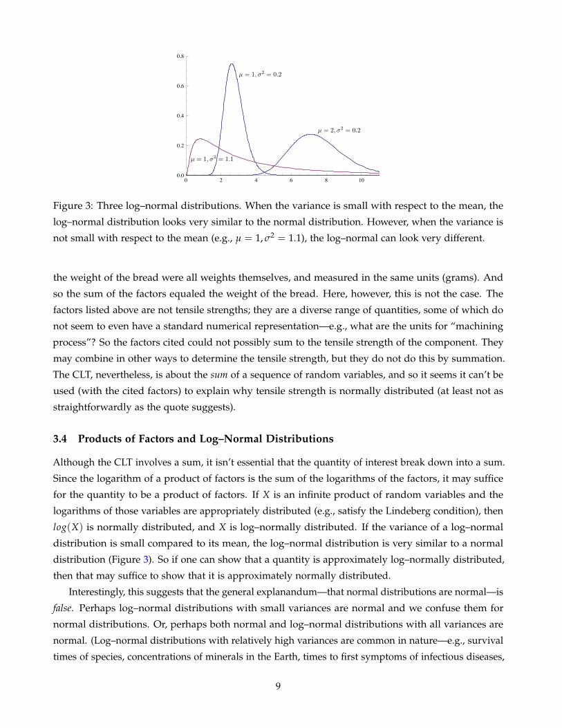
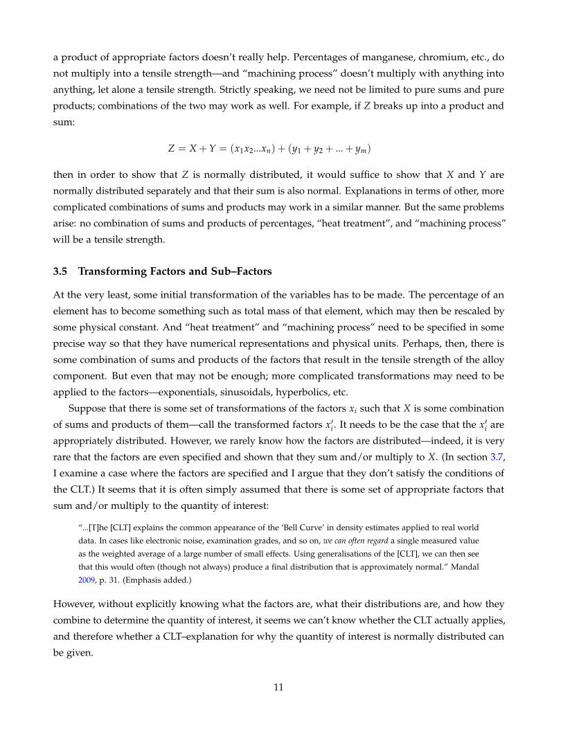
Figure 3: Three log–normal distributions. When the variance is small with respect to the mean, the
log–normal distribution looks very similar to the normal distribution. However, when the variance is
not small with respect to the mean (e.g., µ = 1, σ2 = 1.1), the log–normal can look very different.
the weight of the bread were all weights themselves, and measured in the same units (grams). And
so the sum of the factors equaled the weight of the bread. Here, however, this is not the case. The
factors listed above are not tensile strengths; they are a diverse range of quantities, some of which do
not seem to even have a standard numerical representation—e.g., what are the units for “machining
process”? So the factors cited could not possibly sum to the tensile strength of the component. They
may combine in other ways to determine the tensile strength, but they do not do this by summation.
The CLT, nevertheless, is about the sum of a sequence of random variables, and so it seems it can’t be
used (with the cited factors) to explain why tensile strength is normally distributed (at least not as
straightforwardly as the quote suggests).
3.4 Products of Factors and Log–Normal Distributions
Although the CLT involves a sum, it isn’t essential that the quantity of interest break down into a sum.
Since the logarithm of a product of factors is the sum of the logarithms of the factors, it may suffice
for the quantity to be a product of factors. If X is an infinite product of random variables and the
logarithms of those variables are appropriately distributed (e.g., satisfy the Lindeberg condition), then
log(X) is normally distributed, and X is log–normally distributed. If the variance of a log–normal
distribution is small compared to its mean, the log–normal distribution is very similar to a normal
distribution (Figure 3). So if one can show that a quantity is approximately log–normally distributed,
then that may suffice to show that it is approximately normally distributed.
Interestingly, this suggests that the general explanandum—that normal distributions are normal—is
false. Perhaps log–normal distributions with small variances are normal and we confuse them for
normal distributions. Or, perhaps both normal and log–normal distributions with all variances are
normal. (Log–normal distributions with relatively high variances are common in nature—e.g., survival
times of species, concentrations of minerals in the Earth, times to first symptoms of infectious diseases,
9
numbers of words per sentence, personal incomes.7) Or, perhaps it is only log–normal distributions, of
all variances, that are normal.
Limpert et al. 2001—a study of the use of both distributions in science—found no examples of
original measurements that fit a normal distribution and not a log–normal one (it’s trivial to find cases
of the opposite). The only examples of a normal distribution fitting data better than a log–normal
distribution were cases where the original measurements had been manipulated in some way (ibid, p.
350). Limpert et al. make a strong case that normal distributions are not as common as is typically
assumed, and that log–normal distributions may in fact be more common. They argue that the
multiplication operation is more common in nature than addition:
“Clearly, chemistry and physics are fundamental in life, and the prevailing operation in the laws of these
disciplines is multiplication. In chemistry, for instance, the velocity of a simple reaction depends on the product
of the concentrations of the molecules involved. Equilibrium conditions likewise are governed by factors that
act in a multiplicative way. From this, a major contrast becomes obvious: The reasons governing frequency
distributions in nature usually favor the log–normal, whereas people are in favor of the normal.” Limpert et al.
2001, p. 351.
(By referring to people’s preference for the normal distribution, Limpert et al. are alluding to its
mathematical and conceptual convenience/simplicity.) They also argue that quantities that can’t take
negative values (e.g., people’s heights) can’t be normally distributed, since any normal distribution
will assign positive probability to negative values; however, they can be log–normally distributed,
since log–normal distributions are bounded below by zero (ibid, p. 341 & 342). If they are correct,
then the explananda of the CLT–explanations that one finds in textbooks is false and all of the examples
mentioned so far—bread weights, human heights, bone strengths of wildebeests, tensile strengths,
etc.—are all wrong. All of these quantities would be log–normally distributed, and so, presumably,
their factors multiply together instead of sum together.
Moreover, there have been cases where data that was once thought to be normal actually turned
out to be better accounted for by some other distribution. For example, Peirce 1873 analysed 24 sets
of 500 recordings of times taken for an individual to respond to the production of a sharp sound,
and concluded that the data in each set were all normally distributed. However, Wilson and Hilferty
1929 conducted a reanalysis of the data and found that each of these data sets were not normally
distributed, for various reasons (see also Koenker 2009 for discussion). So the normal distribution may
not be as normal as people previously thought. Indeed, prior to 1900 it seems that it was commonly
accepted that normal distribution was practically universal and was labelled as “the law or errors”,
thus prompting the remark by Poincare quoted at the beginning of this paper. Nevertheless, for the
sake of argument, I will assume that the normal distribution is at least common in nature (see e.g., Frank
2009), and, unless otherwise specified, I will run normal distributions and log–normal distributions
together. My objections to CLT–explanations apply to both cases equally well.
Returning to the example of the tensile strength of the steel alloy, that tensile strength may be
7For more examples see Limpert et al. 2001.
10
a product of appropriate factors doesn’t really help. Percentages of manganese, chromium, etc., do
not multiply into a tensile strength—and “machining process” doesn’t multiply with anything into
anything, let alone a tensile strength. Strictly speaking, we need not be limited to pure sums and pure
products; combinations of the two may work as well. For example, if Z breaks up into a product and
sum:
Z = X + Y = (x1x2...xn) + (y1 + y2 + ... + ym)
then in order to show that Z is normally distributed, it would suffice to show that X and Y are
normally distributed separately and that their sum is also normal. Explanations in terms of other, more
complicated combinations of sums and products may work in a similar manner. But the same problems
arise: no combination of sums and products of percentages, “heat treatment”, and “machining process”
will be a tensile strength.
3.5 Transforming Factors and Sub–Factors
At the very least, some initial transformation of the variables has to be made. The percentage of an
element has to become something such as total mass of that element, which may then be rescaled by
some physical constant. And “heat treatment” and “machining process” need to be specified in some
precise way so that they have numerical representations and physical units. Perhaps, then, there is
some combination of sums and products of the factors that result in the tensile strength of the alloy
component. But even that may not be enough; more complicated transformations may need to be
applied to the factors—exponentials, sinusoidals, hyperbolics, etc.
Suppose that there is some set of transformations of the factors xi such that X is some combination
of sums and products of them—call the transformed factors x′i . It needs to be the case that the x′i are
appropriately distributed. However, we rarely know how the factors are distributed—indeed, it is very
rare that the factors are even specified and shown that they sum and/or multiply to X. (In section 3.7,
I examine a case where the factors are specified and I argue that they don’t satisfy the conditions of
the CLT.) It seems that it is often simply assumed that there is some set of appropriate factors that
sum and/or multiply to the quantity of interest:
“...[T]he [CLT] explains the common appearance of the ‘Bell Curve’ in density estimates applied to real world
data. In cases like electronic noise, examination grades, and so on, we can often regard a single measured value
as the weighted average of a large number of small effects. Using generalisations of the [CLT], we can then see
that this would often (though not always) produce a final distribution that is approximately normal.” Mandal
2009, p. 31. (Emphasis added.)
However, without explicitly knowing what the factors are, what their distributions are, and how they
combine to determine the quantity of interest, it seems we can’t know whether the CLT actually applies,
and therefore whether a CLT–explanation for why the quantity of interest is normally distributed can
be given.
11
140 150 160 170 180 190 200 210Height (cm)
0.000
0.005
0.010
0.015
0.020
0.025
0.030
0.035
0.040
0.045
Pro
babili
ty
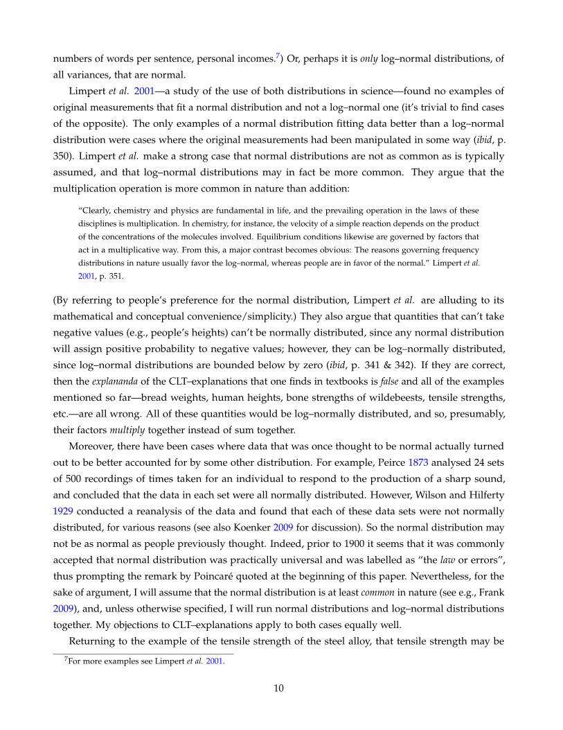
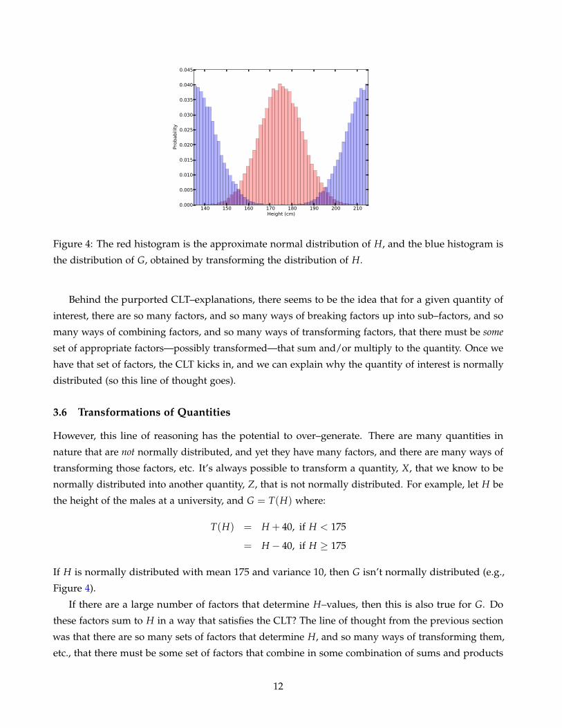
Figure 4: The red histogram is the approximate normal distribution of H, and the blue histogram is
the distribution of G, obtained by transforming the distribution of H.
Behind the purported CLT–explanations, there seems to be the idea that for a given quantity of
interest, there are so many factors, and so many ways of breaking factors up into sub–factors, and so
many ways of combining factors, and so many ways of transforming factors, that there must be some
set of appropriate factors—possibly transformed—that sum and/or multiply to the quantity. Once we
have that set of factors, the CLT kicks in, and we can explain why the quantity of interest is normally
distributed (so this line of thought goes).
3.6 Transformations of Quantities
However, this line of reasoning has the potential to over–generate. There are many quantities in
nature that are not normally distributed, and yet they have many factors, and there are many ways of
transforming those factors, etc. It’s always possible to transform a quantity, X, that we know to be
normally distributed into another quantity, Z, that is not normally distributed. For example, let H be
the height of the males at a university, and G = T(H) where:
T(H) = H + 40, if H < 175
= H − 40, if H ≥ 175
If H is normally distributed with mean 175 and variance 10, then G isn’t normally distributed (e.g.,
Figure 4).
If there are a large number of factors that determine H–values, then this is also true for G. Do
these factors sum to H in a way that satisfies the CLT? The line of thought from the previous section
was that there are so many sets of factors that determine H, and so many ways of transforming them,
etc., that there must be some set of factors that combine in some combination of sums and products
12
to equal H. However, this reasoning seems to apply equally well for G. How, then, can we justify
applying the line of argument to H and not to G?
We know that if H is normally distributed, then G isn’t, since G is T(H) and this transforma-
tion doesn’t preserve normality—nor even approximate normality. This transformation is the final
combination of sums and products of factors that determine G, and so it seems that it’s because
the transformation is part of what determines G that G is not normally distributed. Perhaps this
is what separates H and G. To complete the argument, we need to show that there are no similar
transformations in the determination of H. The problem, though, is that H can be defined in terms of
G as H = T−1(G), where:
T−1(G) = G + 40, if G < 175
= G− 40, if G ≥ 175
T−1 doesn’t preserve normality and it is part of the determination of H, so now the situation for H
and G is reversed. Therefore, there doesn’t seem to be any difference between H and G (that we know
about) that would allow us to justify assuming the conditions of the CLT are true for H and not true
for G. (At this point, one may be tempted to make an appeal to the principle of inference to the best
explanation. If so, see section 3.8.)
One difference between H and G is that H is in some sense “natural” whereas G isn’t.8 However,
the CLT makes no mention of naturalness, so it can’t be the naturalness of H and unnaturalness of G
alone that distinguishes the two quantities. The line of argument would have to be that at least one of
the conditions of the CLT is more plausibly true for a natural variable than for an unnatural one. I
don’t see how such an argument would go, however (similarly for other naturalness–like notions).9
Quantities in nature can always be transformed in these ways. Therefore, there is a sense in which
the very question we are trying to answer—why are normal distributions normal?—is wrong. All
distributions are normal. For every quantity that is normally distributed, there is a another quantity
that is a transformation of the first quantity and is distributed in some other way. The question,
therefore, probably ought to be formulated as something like: why do the quantities in nature that we
tend to focus on tend to be normally distributed? The answer to this question might plausibly involve
the “naturalness” of the quantities that we tend to focus on, and this might allow us to justifiably treat
H and G differently. However, it’s still not clear how the “naturalness” of a random variable could be
used to bolster a CLT–explanation.
8G is a grue–like quantity (Goodman 1955).9Even if such an argument could be made, there could still be a problem. Sometimes H and G will be equally natural
variables:
“[T]he weight of an object depends on the product of its three linear dimensions with its density. Necessarily, if the linear
dimension is precisely normally distributed, the triple product cannot be normally distributed and in fact the resultant
distribution approaches log normality.” Koch 1969, p. 254.
Restricting our attention to natural variables, therefore, doesn’t guarantee there won’t be problematic transformations. (Thanks
to [name removed for blind review] for pointing this out to me.
13
3.7 Quantitative Genetics
In sections 3.2 and 3.3, I discussed examples of CLT–explanations that make only a cursory reference
to the factors that are meant to sum to the quantity of interest and satisfy the conditions of the
CLT. I argued that if we use the factors mentioned in the explanations, then those explanations
simply don’t work. In sections 3.4 and 3.5, I considered two ways in which we might be able to
save—or at least help—the explanations (by allowing combinations of sums and products, and finding
alternative factors through transformations or breaking factors down into sub–factors). In section 3.6, I
discussed a problem with the second strategy for saving the explanations (the problem of potential
over–generation). These arguments, I believe, show that we have little epistemic grounds for giving
such explanations and that we are probably wrong in giving a CLT–explanation for the normality of a
given distribution.
The situation is worse for purported CLT–explanations that make explicit reference to the factors that
determine the quantity of interest. In these cases, very specific and salient factors are mentioned and
play a crucial and central role in their CLT–explanations. The clearest examples of such explanations are
the CLT–explanations for the normal distributions of various phenotypic traits studied in quantitative
genetics.
A common explanation for why people’s heights (for example) are normally distributed is that a
person’s height is largely determined by their genes, and that numerous genes contribute additively to
height, so by the CLT, heights are normally distributed:
“We will now consider the modern explanation of why certain traits, such as heights, are approximately
normally distributed. [...]
We assume that there are many genes that affect the height of an individual. These genes may differ in the
amount of their effects. Thus, we can represent each gene pair by a random variable xi, where the value of the
random variable is the allele pair’s effect on the height of the individual. Thus, for example, if each parent has
two different alleles in the gene pair under consideration, then the offspring has one of four possible pairs of
alleles at this gene location. Now the height of the offspring is a random variable, which can be expressed as
H = x1 + x2 + ... + xn + W
if there are n genes that affect height. (Here, as before, the random variable W denotes non-genetic effects.)
Although n is fixed, if it is fairly large, then Theorem 9.5 [a slightly weaker version of Lindeberg–Feller version
of the CLT] implies that the sum x1 + x2 + ... + xn is approximately normally distributed. Now, if we assume
that the xi’s have a significantly larger cumulative effect than W does, then H is approximately normally
distributed.” Grinstead and Snell 1997, p. 347–8.
Gillespie also sketches a similar explanation:
“There is one very important property of the two–allele model that does change when more loci are added:
The distribution of the genetic effects approaches a normal distribution. [...] There is no a priori reason why the
phenotypic [i.e., height] distribution should be so, well, normal. The Central Limit Theorem from probability
theory does provide a partial explanation. This theorem states that the distribution of the sum of independent
random variables, suitably scaled, approaches a normal distribution as the number of elements in the sum
increases. [...]
14
Of course, the phenotypic distribution also has an environmental component that must itself be approxi-
mately normally distributed if the phenotypic distribution is to be normally distributed. In fact, this appears
to be generally true as judged from an examination of the phenotypic distribution of individuals that are
genetically identical, as occurs, for example, in inbred lines. Perhaps the environmental component is also the
sum of many small random effects that add to produce their effects on the phenotype.” Gillespie 1998, pp.
129–30.
It’s a little difficult to read Gillespie here as it seems he is not completely convinced of this argument.
However, earlier he makes a reference to this two–allele model and writes:
“In the last section of this chapter, we will show how the one–locus model may be replaced with a more
realistic multilocus model, where each locus may have only a couple of alleles. The normality then comes, when
the number of loci is large, from the Central Limit Theorem.” Gillespie 1998, p. 106. (My emphasis.)
There are several reasons to be skeptical of such explanations.10 (I’ll focus on Grinstead and Snell’s
version since it’s more precise and uses a more general version of the CLT.)
First, there is a problem with the construction of random variables whose values are each “allele
pair’s effect on the height of the individual”. Consider an analogy with Wikipedia article lengths. For
some authors, it’s possible to isolate their contribution to the article (e.g., 5 lines of text). However, the
contributions of others cannot be isolated in this way. One author may write one line with completely
false information. This causes another author to delete that one line, and replace it with three more. If
the first author hadn’t written the false information, the second wouldn’t have added the three lines.
Because of this, we can’t associate random variables with each author’s contribution that all have the
same units and sum to the total length of the article. Genes can work in similar ways to determine a
phenotype such as height, and so for the same reason, we can’t associate random variables with each
allele pair’s effect on height that are all measured in the same way and sum to total height.11
The second problem is closely related to the first, but still distinct. Genes can regulate each
other’s expression through gene regulatory networks. They also interact through the developmental
mechanisms that convert gene products into the components of a trait (e.g., muscle tissue). This
means that a gene’s contribution to height can be strongly dependent on the expression of other genes.
However, independence of factors is required for the CLT to apply. Indeed, it’s striking that there
is no mention of the condition of independence in the above passage (or its surrounding text), even
though the version of the CLT that the authors cite (Theorem 9.5) requires it. There are generalisations
of the CLT that allow for some dependencies between factors, so long as other constraints are met
10They originate from, or at least are inspired by, Francis Galton’s work in this area. See Stigler 1986 (ss. 2–3) for a
historical account of the development of such explanations.11Interestingly, the size distribution of featured Wikipedia articles (in bytes) is very well approximated by a log–normal
distribution [url ref]. A standard CLT–explanation of this distribution might be that there are many factors that determine
the size of a featured article—say the contributions of different authors—and these factors are independent and multiply
together to form the total size of each article. Of course, this is not true; at best they might sum together. To run a CLT–style
explanation for the distribution of featured article size one would have to find some set of factors that are appropriately
distributed and multiply to the total byte size of the article (or something that could be transformed to total byte size without
destroying approximate log–normality). It’s not at all clear what those factors would be.
15
(e.g., Hoeffding and Robbins 1948). However, it is by no means clear that genetic factors satisfy these
constraints.
Third, it’s estimated that about 80% of human height is due to genetics (Visscher et al. 2006). The
remaining 20% or so is due to non–genetic factors, such as interactions with the environment and
perhaps epigenetic effects. This means that W’s contribution to H is by no means small. Of course, W
breaks down into sub–factors; however, the same worries apply to those as well—e.g., there might be
interactions between environmental factors and any epigenetic ones.
Fourth, as mentioned earlier, there is some reason to believe that the distribution of heights is better
accounted for by a log–normal distribution. Limpert et al. 2001 point out that quantities that can’t
take non–negative values can’t be normally distributed, and so are more likely to be log–normally
distributed. Heights—and many other traits studied in quantitative genetics—obviously don’t take
negative values, so they may be better understood as being log–normally distributed. In which case, it
might be more reasonable to suppose that at least some of the effects of the gene pairs are multiplicative,
rather than additive.
Some authors have noted that the conditions of the CLT do not generally apply for phenotypic
traits:
“If our random variable is the size of some specified organ that we are observing, the actual size of this organ
in a particular individual may often be regarded as the joint effect of a large number of mutually independent
causes, acting in an ordered sequence during the time of growth of the individual. If these causes simply add
their effects, which are assumed to be random variables, we infer by the central limit theorem that the sum is
asymptotically normally distributed.
In general it does not, however, seem plausible that the causes co–operate by simple addition. It seems
more natural to suppose that each cause gives an impulse, the effect of which depends both on the strength of
the impulse and on the size of the organ already attained at the instant when the impulse is working.” Cramer
1946, p. 219.12
By making some other assumptions, Cramer goes on to argue that the CLT can apply to these impulses
and explain the observed distribution of organ sizes—in particular, Cramer shows how the impulses
may generate a log–normal distribution. However, several of the assumptions that Cramer makes
seem implausible. For example, Cramer supposes that the impulses are independent of each other,
without telling us what they are. (This is also strange because Cramer introduces the argument as an
example of how the CLT can be extended to cases in which the factors are not independent (Cramer
1946, p. 219).)
Hartl and Clark are also aware that the conditions of the CLT are not always satisfied:
“Many measurable quantities in the real world are determined by such sums of independent causes. For exam-
ple, the multiple genetic and environmental factors that determine quantitative traits may be approximately
additive in their effects, so that the central limit theorem is expected to hold. For many characters, the factors
12However, Cramer later writes “[...] it often seems reasonable to regard a random variable observed, e.g., in some
biological investigation as being the total effect of a large number of independence causes, which sum up their effects”
(Cramer 1946, p. 232).
16
appear to multiply in their effects, and in these cases a logarithmic transformation gives a better approximation
to the normal distribution. [...]
The key factor in arriving at a normal distribution is the independence of the component normal factors.
Interdependence of causal factors does occur in quantitative genetics, and this can result in departure from the normal
distribution.” Hartl and Clark 1989, pp. 434–5. (My emphasis.)
They are correct to note that interdependence of causal factors does occur in quantitative genetics;
however, it doesn’t automatically follow that this results in a departure from the normal distribution.13
Interdependent causal factors doesn’t necessarily destroy normality: a quantity that is comprised of
factors that are dependent on each other can quite easily be normally distributed. Interdependence
does, however, have the potential to destroy the applicability of the CLT.
It’s worth noting that Hartl and Clark are perhaps a little optimistic in their claim that many
measurable quantities are determined by sums of independent causes. As an example, they cite genetic
and environmental factors that determined quantitative traits, but we know that such factors often not
independent of each other. Moreover, they seem to be overly optimistic when they write that such
factors “‘may be” approximately additive so the CLT can be “expected to hold”. Of course, the factors
may be approximately additive, but they also may not be. From the fact that they may be approximately
additive, it doesn’t follow that the CLT is expected to hold.
One way to potentially fix things so that the condition of independence is satisfied is to group
dependent terms together and consider them as single terms themselves.14 For example, if x1 and x2
are dependent on each other and so are x4, x5, and x6, then we might proceed as follows:
Then, by definition, the terms in the sum would be independent of each other, thus satisfying the
independence condition. This is the reverse of the proposal in section 3.5, which was to break factors
up into smaller sub–factors. Here, we are combining factors into sup–factors.
However, if there are large groups of factors that are dependent on each other, then some of the
sup–factors will be large, thus violating the Lindeberg condition. Moreover, there may be a “six
degrees of separation” effect that results in very large sup–factors.15 Even if x1 and x2 are independent,
they may nevertheless need to be grouped together. If x3 is dependent on both x1 and x2, then it needs
to be grouped with x1 and x2, which entails that x1 and x2 need to be grouped together (by transitivity
of grouping). In general, if the regulatory network is sufficiently connected in this way, all of the terms,
or at least large groups of them, would have to be grouped together.
One might reply that it may suffice if the independence condition is satisfied only approximately. If
there are only weak dependencies between the genetic factors, then it seems reasonable to expect that
13I don’t believe that Hartl and Clark think that this automatically follows. I’m only emphasising a point that can easily be
missed.14Thanks to Lekki Wood for pointing this out to me.15A.k.a. the Kevin Bacon Game, where in 6 movies or fewer, one links Bacon to another actor by the co–star relation.
17
the CLT applies approximately and that this would result in an approximately normal distribution.16
However, not all of the dependencies between genetic factors are weak; there are clearly some strong
dependencies and the structure of genetic regulator networks is incredibly complex (see e.g., Zhao
2008). So one could resort to the sup–factors argument, but it would also have to be established that
the strong dependencies are few enough and structured in the right way so that the sup–factors are
not so large as to violate the conditions of the CLT. This may in fact be the case; I’m only arguing that
this is what one would have to establish to maintain an approximate application of the CLT. (Note that
one still also has to show that the other conditions are satisfied—e.g., the additivity of the effects.)
3.8 Inference to the Best Explanation
One may respond to the problems that I’ve raised by an appeal to the principle of inference to the best
explanation. If we observe a normally distributed quantity that we know to be determined by a large
set of factors, then by inference to the best explanation, we should infer that those factors satisfy the
conditions of the CLT. In fact, this sort of reasoning can be crucial to understanding the processes that
generate the variety of patterns we observe in nature:
“In general, inference in biology depends critically on understanding the nature of limiting distributions. If a
pattern can only be generated by a very particular hypothesized process, then observing the pattern strongly
suggests that the pattern was created by the hypothesized generative process. [...]” Frank 2009, p. 1564.
Surely, then, it is reasonable to maintain that if we observe that a particular quantity is normally
distributed, and we have no reason to suppose otherwise, we ought to assume (at least as an initial
hypothesis) that the quantity is determined by a set of factors that satisfy the conditions of the CLT.
However, Frank continues:
“By contrast, if the same pattern arises as a limiting distribution from a variety of underlying processes, then
a match between theory and pattern only restricts the underlying generative processes to the broad set that
attracts to the limiting pattern. Inference must always be discussed in relation to the breadth of processes
attracted to a particular pattern.” Frank 2009, p. 1564.
And this is important because:
“We do not know all of the particular generative processes that converge to the Gaussian. Each particular
statement of the central limit theorem provides one specification of the domain of attraction—a subset of the
generative models that do in the limit take on the Gaussian shape.” Frank 2009, p. 1574.
We, therefore, can’t infer that the conditions of any given version of the CLT are satisfied simply on
the basis of observing a normal distribution. We also can’t infer that the conditions of some version of
the CLT are satisfied, because all of the versions of CLT do not exhaust the space of generative models
that lead to the normal (Gaussian) distribution.
16Thanks to Georges Rey and an anonymous reviewer for bringing this reply to my attention.
18
4 Maximum Entropy Explanations
If the previous sections are correct, then the CLT doesn’t explain why normal distributions are normal.
Indeed, it is questionable whether normal distributions really are all that normal: for every normal
distribution, there is a cluster of other distributions that are not normal distributions (section 3.4),
and in many cases throughout the sciences, data that was once thought to be normal turns out to
actually be better accounted for by some other distribution, such as the log–normal (section 3.6). In
addition to this, I’ve argued that in many cases, the CLT fails to explain why particular distributions
are normal—e.g., if heights are normally distributed, then the standard CLT explanations do not work,
and it’s not clear how they could.
Although normal distributions may not be as normal as we once thought they were, they do appear
to be quite common—especially when we restrict our focus to quantities that tend to interest us. The
CLT doesn’t seem to be able to explain this weaker claim, but could there be some other explanation?
Or is it just a coincidence, or simply due to our predilection for simple and symmetric distributions?
Similarly, could there be an interesting explanation for why a given distribution in nature is normal?
One intriguing alternative explanation involves an important mathematical property that the
normal distribution has:
“A further fact, which serves to ’explain’ why it is that this ’order generated out of chaos’ often has the
appearance of a normal distribution, is that out of all distributions having the same variance the normal has
maximum entropy (i.e. the minimum amount of information).” de Finetti 1990, p. 62.
Put more formally: out of all distributions with mean µ, variance σ2, and support over all of R, the
normal distribution, N(µ, σ2), maximises entropy. And the class of normal distributions N(−, σ2) all
maximise entropy subject to the constraints of a fixed variance σ2 and support over R.17
Entropy is a notoriously slippery notion. Its main claims to fame are its roles in information
theory, thermodynamics, and statistical mechanics—although, it’s not clear that it is the one concept
appearing in all of these theories (e.g., Popper 1982, §6). Even as a purely mathematical property of a
probability function, entropy is difficult to define. Perhaps the standard definition is: the entropy of
a continuous distribution p is H(p(x)) = −∫ ∞
∞ p(x) log p(x)dx (e.g., Frank 2009). However, this is a
special case of a more general definition, which includes an (arguably) arbitrary measure function,
m(x): Hm(p(x)) = −∫ ∞
∞ p(x) log p(x)/m(x)dx (see e.g., Jaynes 1968 for a discussion of this definition).
For present purposes, I’ll assume that the entropy of p(x) is H(p(x)). In rough and intuitive terms:
the entropy of a distribution is a measure of how flat and smooth that distribution is; the fatter and
smoother a distribution, the higher its entropy. The flattest and smoothest distribution over R is the
uniform distribution, and the flattest and smoothest distribution over R with a given finite mean and
variance is the normal distribution with that mean and variance.17For more on the history of the normal distribution and its maximum entropy property, see Jaynes 2003, Ch. 7, and
Stigler 1986.
19
This maximum entropy property of the normal distribution makes it an important kind of an
attractor: if we start with some arbitrary distribution and repeatedly perform operations on it so
that it increases in entropy but maintains its mean and variance, then the distribution will approach
the normal distribution. The evolution of the distribution of Sn in the CLT is exactly like this. It
starts off as simply the distribution of x1, but then after the addition of x2 it becomes the distribution
of S2 = (x1 + x2)/√
2, then S3 = (x1 + x2 + x3)/√
3, and so on. Each time another (independent
and identically distributed) xi is added, the entropy is increased, and since there is always the
normalising factor 1/√
i, the variance is maintained, and so the distribution of Sn approaches the
normal distribution. In short, the CLT specifies one particular way in which a sequence of distributions
increase in entropy and remain constant in mean and variance, and thus get attracted to a normal
distribution (Jaynes 2003, p. 221). In fact, as we saw in the previous section, the different versions of
the CLT specify different ways in which distributions can approach the normal distribution (Frank
2009, p. 1574). Each version of the CLT identifies a set of operations (a “generative model”) that
increase entropy and preserve variance (preserving the mean is not necessary since this only controls
the location of the peak of the resulting normal distribution).
As an example of how an ME–explanation might work, consider the tensile strengths from section
3.3 and suppose that they are, in fact, normally distributed. There are many factors that determine
the tensile strength of a component, and they do so in many different and complicated ways. All of
these factors and their interactions are determined by some machining process, which is designed
by some engineers for the purpose of building the components. However, the engineers are not just
interested in building the components, they are also interested in quality control. No machining
process is perfect, so there will always be some error about the desired tensile strength. When building
the machine that produces the components, the engineers will make sure that these errors are within
some acceptable range—they don’t need perfection, just something close to it. This amounts to fixing
the mean (the desired the tensile strength), and the variance (the acceptable range of errors) of the
distribution of tensile strengths. Apart from that, the engineers don’t care what the machine does, and
it will naturally tend to a state of maximal disorder—i.e., a state of maximum entropy—subject to its
engineered constraints. (This is an appeal to something like the second law of thermodynamics, and I
discuss this in more detail below.) The distribution of tensile strengths that maximises entropy subject
to those constraints is a normal distribution, and so that is why the tensile strengths are normally
distributed.
It’s worth considering another example of a completely different kind. Let’s assume that the heights
of a particular human population are normally distributed. There are many factors that determine
a person’s height, and they do so in many different and complicated ways. All of these factors and
their interactions are determined by some evolutionary selection process (natural, sexual, etc.), which
is determined by the population’s environment. The overall selection pressure determines an ideal
20
height,18 but the selection pressure is not perfect, some variability about the ideal won’t matter very
much. In fact, there may even be a selection pressure to maintain some variability to hedge against
fluctuating circumstances in the environment. This amounts to fixing the mean (the ideal height), and
an upper bound on the variance (the variation in the population) of the distribution of heights. Apart
from that, there is no other relevant selection pressure, and the population will naturally tend to a
state of maximal disorder—i.e., a state of maximum entropy—subject to its selection constraints. (This
is another appeal to something like the second law of thermodynamics.) The distribution of heights
that maximises entropy subject to those constraints is a normal distribution, and so that is why the
heights in the population are normally distributed.
If such ME–explanations could be made to work, they would enjoy at least two virtues over CLT
explanations. Firstly, ME–explanations would be more modally robust than an CLT–explanation, in that
the ME–explanations could support a wider range of counterfactuals. This is because ME–explanations
are less committal to the precise details of the aggregation process that converts the factors into the
quantity of interest. Secondly, ME–explanations appear to be appropriately sensitive to one’s choice of
variables. This is because the entropy of a distribution depends on one’s choice of variables—at least
according to the standard formulation, H(p(x)). This causes problems for the Principle of Maximum
Entropy that some have used to determine objective Bayesian priors (see e.g., van Fraassen 1989, p.
303). However, in this context, such dependence on one’s choice of variables may be a virtue, since the
explanandum itself appears to be dependent on one’s choice of variables—i.e., normal distributions
are common only if we carve up the world in the right way.
The are important obstacles that need to be overcome before we can conclude that ME–explanations
save the day, however. Firstly, the examples I gave above assumed that the quantities in question
are normally distributed. But what if they are log-normal, or something else? It seems that ME–
explanations ought to explain other common distributions in nature. Frank 2009 has made a lot
of progress in this direction, demonstrating that several common distributions in nature can be
modeled in terms of processes maximising entropy. However, Frank doesn’t cover an important class
of distributions: the log-normals. One might hope that these could be accounted for by transforming
the log-normal distribution in question into a normal and arguing that entropy is maximised subject
to the appropriate constraints on the transformed variable. It’s not clear how such a story would go,
however, for a quantity such as human height, H—one would have to argue that the variance of ln(H)
is fixed, that the distribution of ln(H) is expected to maximise entropy, and that there are no other
constraints on ln(H).
Secondly, it is by no means clear what entropy is. There are number of interpretations of entropy,
and it is not clear how they can play the appropriate explanatory role. Perhaps the most popular
interpretation is that the entropy of a probability distribution is a measure of the information that an
agent with that distribution has (Frank 2009 appears to have this interpretation in mind). This renders
18In fact, a range of ideal heights would be enough for this example to work.
21
entropy as a property of a subjective probability distribution. But what does how much information
an agent has got to do with distributions of actual frequencies in nature? Something is conceptually
amiss. Since our goal is to explain an actual frequency distribution—e.g., the approximately normal
distribution of human male heights—it’s not clear that this way of thinking about entropy and
probability is satisfactory. (Popper 1982, p. 109, makes a similar point about the explanatory role of
entropy in statistical mechanics.) Whatever the appropriate understanding of entropy is, it seems that
it has to be a physical property and that it can be a property of a diverse range of physical things—from
tensile strengths, to human heights, to bread weights. Moreover, the interpretation of entropy needs to
make it the sort of thing that tends to be maximised. In the examples I gave earlier, I made an appeal
to the tendency of things in nature to increase in disorder, i.e., the second law of thermodynamics.
However, it is not at all clear that the entropy of thermodynamics is the same entropy that normal
distributions maximise.19 One reason to think that it might be, however, is that the Maxwell–Bolztmann
velocity distribution law is the law that the velocities of particles of an ideal gas in a maximum entropy
state are normally distributed. This is by no means a knockdown argument, but it is suggestive.
These issues require much more space than which is available here. ME–explanations may be a way
forward, but much more work needs to be done. My goal is not to argue that ME–explanations are
the correct explanations for why particular distributions are normal/log-normal/etc., or why normal
distributions are common in nature. I only intend to point out that developing ME–explanations in
detail may be a promising alternative explanatory strategy.
5 Conclusion
I began this article with a famous remark regarding the different attitudes experimentalists and
mathematicians have (or at least had) towards the normality of normal distributions. At the end of his
chapter on the normal distribution, Cramer writes of this remark:
“It seems appropriate to comment that both parties are perfectly right, provided that their belief is not too
absolute: mathematical proof tells us that, under certain qualifying conditions, we are justified in expecting a
normal distribution, while statistical experience shows that, in fact, distributions are often approximately normal.”
Cramer 1946, p. 232. (Emphasis in original.)
I have argued that the “certain qualifying conditions” are not satisfied in important cases—e.g., in
quantitative genetics. For other examples (e.g., tensile strengths), I’ve argued that we often have little
reason for assuming that the qualifying conditions are satisfied. I’ve also argued that distributions
are “often approximately normal” only if we carve up the world the right way with our variables.
Any explanation for the normality of normal distributions should take this into account, and CLT–
explanations do not. Moreover, it appears that normal distributions are not as normal as we once
thought they were. There are many documented cases of data initially thought to be normally
19Thanks to Craig Callender for pointing this out to me.
22
distributed turning out to be log-normally distributed (Limpert et al., 2001), or distributed in some
other way (e.g., Wilson and Hilferty 1929).
All of this is not to say that CLT–explanations are never true. To the contrary, the CLT probably
explains why, for example, sample averages tend to be normally distributed. However, note that
sample averages are clearly sums of factors, and are often designed so that those factors are as close to
being independent and identically distributed as possible. My arguments are only intended to show
that often our CLT–explanations fail to be veridical—typically when the quantities in question are more
naturally occurring (e.g., human heights) and have a composition much more complicated than that of
simple sample averages.20
Finally, I’ve suggested that a promising alternative way to explain why a particular quantity is
normally distributed is to appeal to the maximum entropy property that normal distributions have.
This, in turn, may generalise into an explanation for why normal distributions, and many other
distributions, are common in nature.
Acknowledgements
Thanks to Marshall Abrams, Alan Baker, Frederic Brouchard, Rachael Brown, Brett Calcott, Craig
Callender, Lindley Darden, Kenny Easwaran, Branden Fitelson, Alan Hajek, Philippe Huneman, Hanna
Kokko, Roberta Millstein, Georges Rey, Neil Thomason, Lekki Wood, and two anonymous reviewers
for this journal. Special thanks to Branden Fitelson for very detailed and insightful comments on
earlier versions of this paper.
References
Baker, A. (2005). Are There Genuine Mathematical Explanations of Physical Phenomena? Mind 114(454),
223.
Baker, A. (2009). Mathematical Explanation in Science. The British Journal for the Philosophy of Science.
Baker, A. (201X). Science–Driven Mathematical Explanation. Mind. (forthcoming).
Bening, V. and V. Korolev (2002). Generalized Poisson Models and their Applications in Insurance and
Finance, Volume 7. Vsp.
Cramer, H. (1946). Mathematical Methods of Statistics. Asia Publishing House. (Ninth Printing, 1961).
de Finetti, B. (1990). Theory of Probability, Volume 2. John Wiley & Sons Ltd., Chichester.
20Incidentally, that some normal distributions are not explained by the CLT should not be news. For example, the position
of a free particle governed by the Schrodinger equation is a normally distributed variable. Yet there are no factors that
determine the particle’s position (at least, according to “no hidden variables” interpretations of quantum mechanics), let
alone factors that are appropriately distributed, etc.
23
Denny, M. and S. Gaines (2000). Chance in Biology: Using Probability to Explore Nature. Princeton
University Press.
Feller, W. (1971). An Introduction to Probability Theory and its Applications, Volume 2. John Wiley & Sons
and Mei Ya Publications.
Frank, S. A. (2009). The Common Patterns of Nature. Journal of Evolutionary Biology 22.
Galton, F. (1875). Statistics by Intercomparison, with Remarks on the Law of Frequency of Error.
Philosophical Magazine 4(49), 33–46.
Gillespie, J. H. (1998). Population Genetics: A Concise Guide. John Hopkins University Press.
Goodman, N. (1955). Fact, Fiction, and Forecast (1st ed.). Cambridge, MA: Harvard University Press.
Gregersen, E. (Ed.) (2010). The Britannica Guide to Statistics and Probability. Rosen Education Service.
Grinstead, C. and J. Snell (1997). Introduction to Probability. Amer Mathematical Society.
Hartl and Clark (Eds.) (1989). Principles of Population Genetics. Sunderland.
Hoeffding, W. and H. Robbins (1948). The Central Limit Theorem for Dependent Random Variables.
Duke Mathematical Journal 15(3), 773–780.
Jaynes, E. (1968). Prior probabilities. Systems Science and Cybernetics, IEEE Transactions on 4(3), 227–241.
Jaynes, E. (2003). Probability Theory: The Logic of Science. Cambridge University Press Cambridge.
Koch, A. (1969). The logarithm in biology II: Distributions simulating the log-normal. Journal of
Theoretical Biology 23(2), 251–268.
Koenker, R. (2009). The median is the message: Wilson and hilfertys experiments on the law of errors.
The American Statistician 63(1), 20–25.
Leon-Garcia, A. (2008). Probability, Statistics, and Random Processes for Electrical Engineering. Pear-
son/Prentice Hall.
Limpert, E., W. A. Stahel, and M. Abbt (2001). Log–Normal Distributions across the Sciences: Keys
and Clues. BioScience 51(5).
Lyon, A. (201X). Mathematical Explanations of Empirical Facts, and Mathematical Realism. Australasian
Journal of Philosophy. (forthcoming).
Mandal, B. (2009). Global Encyclopaedia of Welfare Economics. Global Vision Publishing House.
Mlodinow, L. (2008). The Drunkard’s Walk. Pantheon Books, New York.
24
Peirce, C. S. (1873). On the theory of errors of observation. Report of the Superintendent of the U.S. Coast
Survery, 200–224.
Popper, K. (1982). Quantum Theory and the Schism in Physics. New Jersey: Rowman and Littlefield.
Roush, M. and W. Webb (2000). Applied Reliability Engineering. Riac.
Stigler, S. (1986). The History of Statistics: The Measurement of Uncertainty Before 1900. Belknap Press.
van Fraassen, B. (1989). Laws and Symmetry. Oxford: Oxford University Press.
Visscher, P., S. Medland, M. Ferreira, K. Morley, G. Zhu, B. Cornes, G. Montgomery, and N. Martin
(2006). Assumption–Free Estimation of Heritability from Genome–Wide Identity–by–Descent Sharing
Between Full Siblings. PLoS Genet 2(3), e41.
Wilson, E. and M. Hilferty (1929). Note on C.S. Peirce’s experimental discussion of the law of errors.
Proceedings of the National Academy of Sciences of the United States of America 15(2), 120.
Zhao, W., E. Serpedin, and E. Dougherty (2008). Inferring connectivity of genetic regulatory networks
using information-theoretic criteria. Computational Biology and Bioinformatics, IEEE/ACM Transactions