Why Are Recessions Associated

With Financial Crises Different?∗

Luca Benati

University of Bern†

Abstract

We use Bayesian time-varying parameters structural VARs with stochastic

volatility to investigate the specific dimensions along which recessions associ-

ated with severe financial crises have historically been different from ‘normal’

recessions, and standard business-cycle fluctuations, in the post-WWII U.S.,

Japan, Euro area, Sweden, and Finland. We identify four structural shocks by

combining a single long-run restriction, to identify a permanent output shock as

in Blanchard and Quah (1989), with three sign restrictions to identify demand-

and supply-side transitory shocks.

Evidence suggests that severe financial crises have systematically been char-

acterized by a negative impact on potential output dynamics, which in two

cases–Japan, following the collapse of the asset prices bubble of the second

half of the 1980s, and Finland, in the early 1990s–appears to have been noth-

ing short of dramatic. With the single exception of the Euro area during the

recent crisis, all financial crises analyzed herein have also been characterized by

a specific pattern of demand non-policy shocks, expansionary during the years

leading up to the crisis, and contractionary following its outbreak. On the

other hand, no other macroeconomic feature has exhibited any systematically

different pattern, during financial crises, compared to standard macroeconomic

fluctuations. Our main conclusion is therefore that, once controlling for the size

of the shocks, financial crises appear to have been broadly similar to standard

macroeconomic fluctuations along many, but not all, dimensions.

Keywords: Financial crises; Bayesian VARs; stochastic volatility; time-varying

parameters; structural VARs; long-run restrictions; sign restrictions; mon-

etary policy; monetary regimes.

∗This paper is an outgrowth of my discussion of M. Bordo and J. Haubrich (2011), ‘Deep Re-cessions, Fast Recoveries, and Financial Crises: Evidence from the American Record’, at the Swiss

National Bank ’s research conference ‘Policy Challenges and Developments in Monetary Economics’

(Zurich, 23-24 September, 2011). I wish to thank Joseph Haubrich for useful conversations. Usual

disclaimers apply.†Department of Economics, University of Bern, Schanzeneckstrasse 1, CH-3001 Bern, Switzer-

land. Email: luca.benati@vwi.unibe.ch

1

1 Introduction

Reinhart and Rogoff’s work on the history of financial crises1 has established two

key facts. First, financial crisis, which, during the years leading up to the Great

Recession, had routinely been regarded as a largely ‘out-of-date’ topic, have been a

regular feature of macroeconomic fluctuations for hundreds of years. Second, severe

financial crises have typically had dramatic and long-lasting macroeconomic effects,

with large and protracted falls in output, and sizeable increases in the unemployment

rate. As Reinhart and Rogoff (henceforth, RR) put it,2

‘[...] the aftermath of banking crises is associated with profound declines

in output and employment. The unemployment rate rises an average of 7

percentage points during the down phase of the cycle, which lasts on average

more than four years. Output falls (from peak to through) more than 9 per

cent on average, although the duration of the downturn, averaging roughly two

years, is considerably shorter than that of unemployment.’

Although groundbreaking, RR’s work, being exclusively based on either the analy-

sis of the raw data, or simple regression techniques, cannot provide answers to impor-

tant questions concerning the specific dimensions along which recessions associated

with financial crises have historically been different from ‘normal’ recessions and,

more generally, from standard business-cycle fluctuations. In particular,

• ‘Have financial crises simply been characterized by larger shocks, or is it possibleto detect changes in the relative importance of different types of shocks?’

• ‘Once controlling for the size of the shocks, is it possible to detect differencesin the transmission mechanism, compared to standard macroeconomic fluctua-

tions?’

• ‘More generally, is it possible to detect a set of features which have consistentlybeen common to all financial crises, across countries and, possibly, across mon-

etary regimes?’

The very nature of these questions implies that the methodology to be used in

order to successfully tackle them should allow for time-variation in both the size of

the shocks, and the way in which they propagate through the economy, and it should

allow for the identification of a set of structural shocks.

1See, first and foremost, Reinhart and Rogoff (2009).2See RR (2009, p. 224).

2

1.1 This paper: methodology and main results

In this paper we use Bayesian time-varying parameters structural VARs with stochas-

tic volatility to investigate the specific dimensions along which recessions associated

with severe financial crises have historically been different from normal recessions, and

from standard business-cycle fluctuations, in the post-WWII United States, Japan,

Euro area, Sweden, and Finland. We identify four structural shocks by combining

a single long-run restriction, to identify a permanent output shock as in Blanchard

and Quah (1989), with three sign restrictions to identify demand- and supply-side

transitory shocks.

Our main results can be summarized as follows.

First, a consistent feature among all the severe financial crises considered herein

is a non-negligible negative impact on potential output dynamics.3 In two cases–

Japan and Finland in the early 1990s–the impact appears to have been nothing short

of dramatic, with an obvious, significant decrease in Japan’s trend output growth

following the crisis; and a sizeable permanent output loss, but no significant change

in trend output growth, in Finland. As for the recent crisis, its impact appears

to have been comparatively mild in the United States and Sweden, and to have

instead been quite significant in Japan, with (based on median estimates) a sizeable

one-off permanent output loss equal to 3.6 per cent of potential GDP. The impact

on the Euro area’s potential output dynamics, on the other hand, appears to have

been intermediate between these extremes, with potential GDP estimated to have

temporarily decreased by 2.3 per cent from the peak of 2008Q1 to the trough of

2009Q1, before resuming its upward trend. An important point to stress, however,

is that–with the single exception of Japan’s crisis of the early 1990s–our evidence

does not suggest that, under this respect, financial crises are in any way ‘special’,

compared to normal recessions. Rather, our results are compatible with the notion

that financial crises have been characterized by sizeable negative effects on potential

output dynamics simply because, historically, the have been associated with extremely

deep recessions, which have ended up ‘blasting away pieces of the economy’. Both in

the United States and in the Euro area, for example, the recessions associated with the

disinflations of the early 1980s, which had been significantly less severe than those

associated with the recent financial crisis, had indeed exhibited, according to our

results, vastly milder, but still statistically significant negative effects on potential

output dynamics. To put it differently, with the single exception of the Japanese

3Although, throughout the entire paper, we talk about the ‘negative impact’ of financial crises on

potential output dynamics, it is important to keep in mind that, strictly speaking, the methodology

used herein does not allow us to establish a causal relationship between the crisis and concurrent

and/or subsequent developments in the evolution of potential output. Our circumstantial evidence,

however–with all the financial crisis analyzed herein having systematically been associated with

either a temporary or a permanent deterioration in the evolution of potential output–is remark-

ably strong, and it naturally suggests that financial crises have been the underlying cause of such

deterioration.

3

financial crisis of the early 1990s–which impacted on potential output growth, and is

therefore in a league of its own–what seems to matter is the depth of the recession,

rather than the fact that it has been associated with a financial crisis.

Second, in most, but not all cases (with the most notable exception being the

Euro area during the recent crisis), demand non-policy shocks–which, within the

present context, should be expected to capture credit market disturbances–displayed

a consistent pattern, expansionary in the run-up to the crisis, and contractionary

following its outbreak.

Third, quite surprisingly, a temporary increase in macroeconomic volatility does

not appear to have been a robust common feature of financial crises. For example, for

neither Japan, Finland, nor Sweden the financial crises of the early 1990s had been

associated with any significant change in the volatility of reduced-form innovations

to real GDP growth. This is especially noteworthy for Japan and Finland, which,

during those years, experienced a dramatic deceleration in potential output growth,

and a prolonged and sizeable fall in the level of potential output, respectively.

Fourth, in a few cases, severe financial crises appear to have been characterized by

a temporary increase in the persistence of output growth. This is especially apparent

for the U.S. during the recent crisis, and for Sweden in the early 1990s. This implies

that these crises have been associated with deep and prolonged recessions not only

because (trivially) they have been characterized by a sequence of comparatively large

negative shocks, but also because–conditional on those shocks–output growth has

exhibited a systematic tendency to revert to the mean more slowly than under normal

circumstances. On the other hand, once again, a temporary increase in output growth

persistence has clearly not been a robust common feature of financial crises.

Fifth, in the majority of cases impulse-response functions to the identified struc-

tural shocks do not exhibit any systematically different pattern compared to normal

periods, thus suggesting that, historically, financial crises have not been associated

with changes in the way structural disturbances propagate through the economy.

Overall, international evidence for the post-WWII period therefore suggests that,

beyond having been characterized by sequences of comparatively large contractionary

shocks, severe financial crises have not exhibited a widespread pattern of systematic

differences compared to standard macroeconomic fluctuations: as we pointed out,

once controlling for the size of the shocks the only features that still stands out

is a non-negligible, and sometimes significant negative impact on potential output

dynamics.

1.2 Related literature

In recent years, the persistent, negative impact on output of traumatic macroeconomic

events such as banking and currency crises has been extensively documented in the

literature. Based on data for 190 countries for the period 1960-2001, Cerra and

Saxena (2008) showed how banking crises have uniformly been associated with large

4

and prolonged falls in output for all the country groups and geographical areas they

considered. In particular, based on their full sample they estimated the change in

output following a banking crisis to reach a plateau equal to almost -8 per cent at the

10-year horizon. An intrinsic limitation of Cerra and Saxena’s work, however, is that,

being based on reduced-form methods, it can only estimate the average magnitude,

within a specific group of countries, of the fall in output associated with a financial

crisis, but it cannot identify either the nature of the shocks at the origin of the crises

themselves, or the specific dimensions along which recessions associated with financial

crises differ from ‘normal’ recessions (apart from the size and duration of the fall in

output).

In their influential history of financial crises over the last several centuries, RR

(2009) documented systematic, large and persistent falls in real per capita GDP in the

immediate aftermath of severe banking crises, equal, on average, to -9.3 per cent.4 As

previously pointed out, however, RR’s entire work is based on the analysis of the raw

data, and, exactly as Cerra and Saxena (2008), it cannot therefore provide answers

to the three questions we posed at the beginning.

Two papers have questioned, for the United States, RR’s contention that financial

crises have historically been fundamentally different from normal recessions. Based on

both the analysis of the raw data, and simple reduced-form regressions, Lopez-Salido

and Nelson (2010) argued that one of RR’s two previously mentioned key findings–

recessions associated with financial crises have been especially prolonged and drawn-

out–does not hold for the post-WWII U.S.. A limitation of Lopez-Salido and Nelson’s

(henceforth, LSN) analysis, beyond being based on very simple regression methods,

is however that they do not consider the Great Recession (which, at the time of their

writing, was still ongoing). Indeed, as I discuss more extensively in Section 3 below,

for the post-WWII U.S. before the Great Recession I estimate, in line with LSN,

essentially no change over time in the persistence of output growth, but crucially,

and in line with RR, I identify a sizeable increase in persistence associated with the

Great Recession.

Bordo and Haubrich (2011)’s work is, both conceptually and methodologically,

very close to LSN’s, with the key difference being that it analyzes U.S. data since the

second half of the XIX century. Their main conclusion is that ‘[. . . ] recessions asso-

ciated with financial crises are generally followed by rapid recoveries..’ They identify

three exceptions to this pattern: ‘[...] the recovery from the Great Contraction in the

1930s; the recovery after the recession of the early 1990s and the present recovery

[that is, the recovery from the Great Recession].’ As for LSN, an intrinsic limita-

tion of Bordo and Haubrich’s analysis is that, being based on very simple regression

methods, it cannot either identify structural shocks, or explore the specific dimensions

along which recessions associated with financial crises have been idiosyncratic.

Finally, Stock and Watson (2012) focus on the 2007-2009 U.S. recession based

on a fixed-coefficients dynamic factor model with 200 variables. One of their key

4See RR (2009, pages 229-230, and in particular Figure 14.4).

5

conclusions is that

‘[...] although many of the events of the 2007-2009 collapse were unprece-

dented, their net effect was to produce macro shocks that were larger versions

of shocks previously experienced, to which the economy responded in an his-

torically predictable way.’

As previously pointed out, this is in line with most (but not all) of the results of

the present work. An intrinsic limitation of either LSN (2010), Bordo and Haubrich

(2011), or Stock and Watson (2012) is their exclusive focus on the United States. It

is indeed an open question to which extent the U.S. experience can be regarded as

representative of the broader experience with financial crises worldwide. Along one

conceptually related dimension–the size of the unit root in GNP–Cogley (1990)

showed for example that the U.S. should be regarded, when seen from an interna-

tional perspective, as an outlier, with the size of the permanent component of output

estimated to have been markedly smaller than for all other countries he considered.

This implies that exploring this issue also based on data for countries other than the

U.S. should be regarded, at the very least, as a robustness check on the results one

obtains based on U.S. data. This is the fundamental reason why, in the spirit of

RR (2009), in the present work I have chosen to use data for as many countries as

possible.

The only other paper I am aware of to adopt an international perspective is Papell

and Prodan (2011). Papell and Prodan (henceforth, PP) apply break tests within a

univariate context in order to investigate whether severe recessions associated with

financial crises have a permanent impact on output, and, if they don’t, whether under

these circumstances output returns to potential more slowly than during ‘normal’

recessions. Overall, evidence for episodes comparable with the U.S. Great Recession

suggests that, although output ultimately returns to the pre-crisis trend, on average

slumps last about nine years.

The paper is organised as follows. The next section describes the Bayesian

methodology we use to estimate the time-varying parameters VARs with stochas-

tic volatility, the identification strategy, and the methodology for computing the

structural VAR’s impact matrix. Section 3 discusses the set of features which have

historically been common across most severe financial crises, whereas Section 4 fo-

cuses on individual financial crises’ idiosyncratic aspects. Section 5 concludes, and

discusses directions for future research.

6

2 Methodology

2.1 A Bayesian time-varying parameter VAR with stochastic

volatility

In what follows we will work with the following time-varying parameters VAR(p)

model:

= 0 +1−1 + +− + ≡ 0 + (1)

where the notation is obvious, and is defined as ≡ [∆ ]0, where is

the logarithm of real GDP; is inflation, computed as the log-difference of the GDP

deflator; is a short-term interest rate (in the case of the United States, the Federal

Funds rate), which is quoted at a non-annualized rate in order to make its scale exactly

comparable to that of inflation;5 and is a stationary variable capturing the state of

the business-cycle. For the United States, following Blanchard and Quah (1989), is

the civilian unemployment rate. For all other countries, for which the assumption of

stationarity of the unemployment rate is questionable,6 is the consumption/output

ratio.7 The key rationale for including in the VAR either the unemployment rate or

the consumption/output ratio is in order be able to effectively disentangle permanent

and transitory output shocks. The VAR we estimate for the U.S. is an expanded

version of the one originally estimated by Blanchard and Quah (1989), which only

included the log-difference of output and the unemployment rate, whereas the one we

estimate for all other countries is an expanded version of one of the models estimated

by Cochrane (1994), which only included the log-difference of output and the log

of the consumption/GDP ratio.8 In both papers, the unemployment rate and the

log of the consumption/output ratio, respectively, were included because of their

strong informational content on the state of the business cycle and, therefore, on the

5So, to be clear, if is the relevant short-term rate–with its scale such that, e.g., a ten per

cent rate is represented as 10.0– is computed as =(1+/100)14-1.

6Although the unemployment rate is bounded between 0 and 1, so that, strictly speaking, it

cannot be non-stationary, first, for all the countries considered herein (except the United States),

bootstrapped p-values for Augmented Dickey-Fuller tests without trend clearly point towards the

unemployment rate being I(1). (These results are not reported here for reasons of space, but they

are available from the author upoin request.) Second, even based on simple ‘eyeball econometrics’,

for all countries except the U.S. the unemployment rate exhibits an obvious extent of permanent

variation. In the Euro area, for example, it has increased from about 2-3 per cent in the early 1970s

to a new equilibrium around 9-10 per cent which has prevailed over the last 2 decades.7Results based on the logarithm of the consumption/output ratio are near-identical to those

based on the consumption/output ratio. These results are not reported here for reasons of space,

but they are available from the author upon request.8As discussed by Cochrane (1994, see in particular the Appendix) the benchmark model he esti-

mates in the paper–a cointegrated VAR for the log-differences of real GNP and real consumption–

can be re-cast in several alternative ways. One of them is as a VAR for the log-difference of real GNP

and the logarithm of the consumption/output ratio. See also Cogley (2005), who, conceptually in

line with the present work, estimated a Bayesian time-varying parameters VAR for output growth

and the logarithm of the consumption/output ratio.

7

transitory component of output.9 For a complete description of the data and of their

sources, see Appendix A.

The overall sample periods are 1954Q3-2012Q1 for the United States, 1963Q1-

2012Q1 for the Euro area, 1970Q1-2011Q4 for Finland, 1955Q2-2011Q4 for Japan,

and 1980Q1-2011Q4 for Sweden. For all countries, however, we use the first 10 years

of data in order to compute the Bayesian priors, so that the effective sample periods

start in 1964Q3 for the United States, in 1980Q1 for the Euro area and Finland, in

1965Q2 for Japan, and in 1990Q1 for Sweden. As it is customary in the literature on

Bayesian time-varying parameters VARs,10 we set the lag order to p=2.

The VAR’s time-varying parameters, collected in the vector , are postulated to

evolve according to

( | −1, ) = () ( | −1, ) (2)

with () being an indicator function rejecting unstable draws–thus enforcing a

stationarity constraint on the VAR–and with ( | −1, ) given by = −1 + (3)

with ∼ (0 ). The VAR’s reduced-form innovations in (1) are postulated to

be zero-mean normally distributed, with time-varying covariance matrix Ω which,

following established practice, we factor as

Var() ≡ Ω = −1 (−1 )

0 (4)

The time-varying matrices and are defined as:

≡

⎡⎢⎢⎣1 0 0 0

0 2 0 0

0 0 3 0

0 0 0 4

⎤⎥⎥⎦ ≡

⎡⎢⎢⎣1 0 0 0

21 1 0 0

31 32 1 0

41 42 43 1

⎤⎥⎥⎦ (5)

with the evolving as geometric random walks,

ln = ln−1 + (6)

For future reference, we define ≡ [1, 2 3 4]0. Following Primiceri (2005),we postulate the non-zero and non-one elements of the matrix –which we collect

in the vector ≡ [21, 31, ..., 43]0–to evolve as driftless random walks,

= −1 + , (7)

9As extensively discussed by Cochrane (1994), the strong informational content of the consump-

tion/output ratio for the transitory component of output is a direct consequence of the permanent

income hypothesis under the assumption of rational expectations, and of frictionsless access to bor-

rowing on the part of consumers.10See e.g. Cogley and Sargent (2002), Cogley and Sargent (2005), Primiceri (2005), Benati (2008),

and Benati and Goodhart (2011).

8

and we assume the vector [0, 0,

0,

0]0 to be distributed as⎡⎢⎢⎣

⎤⎥⎥⎦ ∼ (0 ) , with =

⎡⎢⎢⎣4 0 0 0

0 0 0

0 0 0

0 0 0

⎤⎥⎥⎦ and =

⎡⎢⎢⎣21 0 0 0

0 22 0 0

0 0 23 0

0 0 0 24

⎤⎥⎥⎦(8)

where is such that ≡ −1 12 . As discussed by Primiceri (2005), there are

two justifications for assuming a block-diagonal structure for . First, parsimony, as

the model is already quite heavily parameterized. Second, ‘allowing for a completely

generic correlation structure among different sources of uncertainty would preclude

any structural interpretation of the innovations’.11 Finally, following, again, Primiceri

(2005) we adopt the additional simplifying assumption of postulating a block-diagonal

structure for , too–namely

≡ Var ( ) = Var ( ) =⎡⎣ 1 01×2 01×302×1 2 02×303×1 03×2 3

⎤⎦ (9)

with 1 ≡ Var( 21), 2 ≡ Var([ 31 32]0), and 3 ≡ Var([ 41 42 43]0), thusimplying that the non-zero and non-one elements of belonging to different rows

evolve independently. As discussed in Primiceri (2005, Appendix A.2), this assump-

tion drastically simplifies inference, as it allows to do Gibbs sampling on the non-zero

and non-one elements of equation by equation.

2.2 Estimation

We estimate (1)-(9) via standard Bayesian methods. Appendix B discusses our choices

for the priors–which are standard–and the Markov-Chain Monte Carlo (henceforth,

MCMC) algorithm we use to simulate the posterior distribution of the hyperparame-

ters and the states conditional on the data.

2.2.1 Imposing constraints on the VAR’s time-varying means

The fact that both the unemployment rate and the consumption/output ratio are,

by construction, bounded between 0 and 1, whereas the short rate cannot take neg-

ative values, automatically implies that the corresponding time-varying means (that

is: local equilibrium levels) implied by the VAR ought to satisfy those very same con-

straints at each point in time. In estimation we impose such constraints by rejecting

each MCMC draw for which either (i) the VAR’s mean for the unemployment rate

11Primiceri (2005, pp. 6-7).

9

(or the consumption/output ratio) is outside the [0, 1] interval for at least one quar-

ter, or (ii) the mean for the short rate is negative for at least one quarter.12 This

way of imposing constraints on the VAR’s means was used by Cogley and Sargent

(2002) to impose a non-negativity constraint on the mean for the short rate, and,

from a conceptual point of view, it is akin to the previously discussed imposition of

a stationarity constraint on the VAR on a period-by-period basis.

An alternative way of imposing the relevant constraint on the means for the unem-

ployment rate and the consumption/output ratio would have been to work with their

logit transformations.13 For the consumption/output ratio this would have produced

results near-identical to those reported below, since, for all countries we consider,

the consumption/output ratio and its logit transformation–once demeaned, and di-

vided by their respective standard deviations–are near-numerically identical to each

other. Intuitively, this is due to the fact that, for values which are sufficiently far

away from either 0 or 1, the logit transformation is very close to being linear, and

only for values close to the two boundaries it becomes highly non-linear. For the U.S.

unemployment rate, however, results would likely have been different, because, even

when standardized, the unemployment rate and its logit transformation differ from

each other to a non-negligible extent for several quarters. (This is due to the previ-

ously mentioned high non-linearity of the logit transformation for values sufficiently

close to either 0 or 1.) In particular–and crucially for the present purposes–during

the Great Recession the logit of the U.S. unemployment rate increased proportion-

ally less than the unemployment rate itself, which would have misleadingly pointed

towards a milder recession than it actually was the case. As a consequence, had we

worked, for the United States, with the logit of the unemployment rate, we would

likely have under-estimated the extent of the transitory fluctuation of output dur-

ing that episode, and we would therefore have likely over-estimated the relevance of

permanent output shocks.

2.3 Identification

2.3.1 The permanent output shock

We identify four shocks. Following Blanchard and Quah (1989), the first shock is

defined as the only one exerting a permanent impact on log output, and it is identified

via a long-run restriction.

Given the key role played by such permanent-transitory decomposition in our

analysis, it is important to have some corroborating evidence on the reliability of the

12So, to be clear, given the sequential nature of the MCMC algorithm used herein, if all of the

relevant constraints are satisfied for the j -th draw we move to (j+1)-th draw. Otherwise, we reject

the j -th draw and we keep drawing until we get a draw which satisfies all of the relevant constraints

on the VAR’s means for each quarter. Only at that point we move to (j+1)-th draw.13Indeed, Cogley and Sargent (2002) impose such a constraint on the unemployment rate’s mean

by working with the logit of the unemployment rate.

10

Blanchard-Quah identification scheme when applied to our time-varying parameters

VARs. To put it differently, what are the properties of the identified permanent and

transitory output shocks? Do they look ‘reasonable’ when seen from the perspective

of reliable information extraneous to the VARs? The left-hand side panel of Figure 1

provides informal evidence on this, by showing, for the United States, the median and

the one-standard deviation percentiles of the posterior distribution of the estimated

transitory components of log real GDP, together with the output gap estimate implied

by the Congressional Budget Office (henceforth, CBO) estimate of potential GDP.14

The CBO and VAR-implied estimates of the output gap strongly co-move and are,

most of the time, numerically quite close. The main exceptions are the second half

of the 1960s, when the CBO estimate, peaking at around 6 per cent, is significantly

larger than the one generated by the VAR, and the period following the collapse of

Lehman Brothers, with the VAR pointing towards a smaller transitory fluctuation

(and therefore, a correspondingly larger permanent one) than the one implied by the

CBO estimate. As we will discuss in Section 3, indeed, a non-negligible impact on

potential output dynamics appears to have been, historically, a feature common to

all the severe financial crises analyzed herein.

Overall, we regard the evidence reported in the left-hand side panel of Figure 1 as

reassuring, as, for the only country for which there exists an authoritative output gap

estimate which can be used as a benchmark,15 the transitory component of output

generated by the Blanchard-Quah decomposition applied to the time-varying VAR

appears as entirely reasonable.

The other two panels of Figure 1 report estimates of the transitory component of

output for Japan and the Euro area, whereas the second column of Figure 2 shows the

corresponding estimates for Finland and Sweden. Overall, VAR-generated estimates

of the output gap appear as entirely reasonable, and they accord well with post-

WWII macroeconomic history. For Japan, for example, we estimate (based on median

estimates) a sizeable output gap, equal to about 3 per cent, at the peak of the bubble,

at the end of the 1980s-beginning of the 1990s, and, in line with the conventional

wisdom of a prolonged recession during subsequent years, a consistently negative

output gap for most of the quarters between the early 1990s and the beginning of the

financial crisis. For the Euro area, the output gap is estimated to have decreased,

during the financial crisis, from a peak of 1.6 per cent in 2008Q1 to a trough of -2.6

per cent in 2010Q2, and to have subsequently increased, reaching a value of -1.6 per

14So, to be clear, what is labelled in the Figure as the ‘CBO estimate of the output gap’ has

been computed as the percentage difference between GDPC96 (‘Real Gross Domestic Product, 3

Decimal, Seasonally Adjusted Annual Rate, Billions of Chained 2005 Dollars’) and GDPPOT (‘Real

Potential Gross Domestic Product, U.S. Congress: Congressional Budget Office, Billions of Chained

2005 Dollars’). It is important to stress that both GDPC96 and GDPPOT are expressed in the

same units, and so they are exactly comparable.15For the Euro area, the only output gap estimate we are aware of is the European Central Bank ’s

own internal estimate, which, however, is not disseminated externally. For other countries, we are

not aware of any available official estimate.

11

cent at the end of the sample, in 2012Q1.

2.3.2 The three transitory output shocks

The other three shocks–which, by construction, only exert a transitory impact on

output–are identified based on the standard set of sign restrictions reported in the

following table.

Shock:

Variable: Output growth ≤ 0 ≥ 0 ≥ 0

Inflation ≤ 0 ≥ 0 ≤ 0Unemployment rate, or

consumption/output ratio ≥ 0 ≤ 0 ≤ 0Short rate ≥ 0 ≥ 0 ?

? = left unconstrained

An interest rate shock ( ) is identified based on the restriction that it exerts

a non-negative impact on both the interest rate and either the unemployment rate

or the consumption/output ratio, and a non-positive impact on inflation and output

growth. A demand non-interest rate shock ( ) is postulated to have a non-negative

impact on either output growth, inflation, and the interest rate, and a non-positive

impact on either the unemployment rate or the consumption/output ratio. Finally,

a transitory supply shock ( ) is disentangled from the other two because it is

postulated to be the only shock inducing a negative co-movement between inflation

and output growth, and a positive co-movement between inflation and either the

unemployment rate or the consumption/output ratio.

In what follows we impose these sign restrictions only on impact. The reason for

doing this is that, as stressed by Canova and Paustian (2011), whereas sign restrictions

on impact are, in general, robust–in the specific sense that they hold for the vast

majority of sub-classes within a specific class of DSGE models, and for the vast

majority of plausible parameters’ configurations–restrictions at longer horizons are

instead, as they put it, ‘whimsical’, meaning that they are hard to pin down, and in

general, they are not robust across sub-classes of models, and for alternative plausible

parameters’ configurations.16

16One obvious limitation of imposing the sign restrictions only on impact is that we are here using

a comparatively limited amount of information in order to achieve identification. As a consequence,

our results necessarily end up being less sharp than they could have been had we been reasonably

confident about imposing a specific pattern of sign restrictions at horizons greater than zero. This

compounds a well-known limitation of sign restrictions which has been extensively discussed by

Fry and Pagan (2007): as these authors stress, sign restrictions are intrinsically ‘weak information’,

since they are based on the notion of uniquely imposing a specific pattern of signs on the IRFs.

The rationale behind our decision of imposing sign restrictions only on impact is that it is better to

12

2.3.3 Rationale behind the postulated sign restrictions

Transitory output shocks should logically be expected to move output and the unem-

ployment rate in opposite directions–for evidence supporting this position, see the

IRFs of output and the unemplyment rate to a transitory output shock estimated by

Blanchard and Quah (1989). As for the response of the consumption/output ratio,

the negative co-movement of this variable with output in response to transitory out-

put shocks is a direct consequence of the permanent income hypothesis (on this, see

the extensive discussion in Cochrane, 1994).17 This implies that, in discussing the

rationales behind the postulated sign restrictions, we can ignore, from now on, the

unemployment rate and the consumption/output ratio, and we can exclusively focus

on output growth, inflation, and the short rate.

The sign restrictions reported in the previous table are the same used, e.g., by

Benati (2008), Benati and Goodhart (2011), and Benati and Lubik (2012), and can

be motivated in two diffent ways. First, they naturally arise from a simple aggre-

gate demand-aggregate supply framework. Second, they are the same as the ‘robust

sign restrictions’ reported by Canova and Paustian (2011) in their Table 2 for their

benchmark DSGE model featuring sticky prices, sticky wages, and several standard

frictions (see the column labelled as ‘M ’). Specifically, the signs we impose for the

impacts of on the short rate, inflation, and output growth are the same as those

for Canova and Paustian’s ‘monetary shock’, whereas the signs we impose for are

the same as those for their ‘taste shock’. Finally, as for , the opposite pattern of

signs it induces on impact on inflation and output growth holds for either of Canova

and Paustian’s ‘markup’ and ‘technology’ shocks.18

2.3.4 What about credit market disturbances?

As I also discuss in Section 2.5 below, credit market disturbances should logically

be expected to end up being classified, within the present taxonomy of shocks, as

demand non-interest rate shocks.19 A positive shock to credit spreads, for example,

impose a limited amount of information about which we can be reasonably confident than a greater

amount of information about which we have limited confidence.17Whereas a permanent output shock moves output and consumption in lockstep, thus leaving

their ratio unaffected, a transitory shock only impacts upon output, and it instead leaves consump-

tion unaffected. As a result, transitory output shocks, whatever their specific nature and origin,

necessarily induce a negative co-movement between output and the consumption/output ratio.18Canova and Paustian’s Table 2 also reports robust sign restrictions for the impacts of the

‘markup’ and ‘technology’ shocks on the short rate. However, since such restriction is not necessary

in order to disentangle from the other two transitory output shocks (as we pointed out, is

the only shock inducing a negative co-movement between inflation and outpout growth), we have

preferred not to impose it.19On the other hand, credit market disturbances associated with financial institutions going out

of business, or even with a permanent ‘shrinking’ of the size of the financial sector (which appears

to have been the case, e.g., in the United Kingdom during the recent financial crisis) would have

a permanent impact on output, and would therefore end up being classified as permanent output

13

should be expected to have a non-positive impact on both inflation and output growth.

As for the short rate, the impact should also be expected to be non-positive, based

on the rationale that, facing such a shock, the central bank may choose to to do

nothing–in which case the short rate would remain unchanged–or (which is more

likely, especially in the light of the recent financial crisis) it may decide to counter

the contractionary impact of the increase in credit spreads by cutting the policy rate.

On the other hand, it is highly implausible that, in the face of such a shock, the

monetary authority may somehow decide to compound its contractionary impact by

increasing the policy rate.

This implies that, e.g., if credit market disturbances played a ‘dominant’ role

during financial crises–in terms of the fractions of the forecast error variance of

macroeconomic variables explained by such shocks–this should be expected to show

up in an increase in the importance of demand non-policy shocks. On the other hand,

if, once controlling for changes in the volatility of all shocks, features pertaining to

demand non-policy shocks did not exhibit, during financial crises, significant differ-

ences compared to standard busines cycle fluctuations, this would suggest that, under

this specific dimension, financial crises differ from normal periods only in terms of

the greater volatility of shocks.

2.4 Computing the VAR’s structural impact matrix

For each quarter, and for each draw from the ergodic distribution, we compute the

time-varying structural impact matrix, 0 by combining the methodology proposed

by Rubio-Ramirez, Waggoner, and Zha (2005) for imposing sign restrictions 20 and

the procedure proposed by Gali and Gambetti (2009) to impose long-run restrictions

within a time-varying parameters VAR context. Specifically, let Ω = 0 be the

eigenvalue-eigenvector decomposition of the VAR’s time-varying covariance matrix

Ω, and let 0 ≡ 12 . We draw an × matrix, , from the (0, 1) distri-

bution, we take the decomposition of –that is, we compute matrices and

such that = · –and we compute the time-varying structural impact matrixas 0=0 ·0. Following Gali and Gambetti (2009, Section II), we then computea local approximation to the matrix of the cumulative impulse-response functions

(henceforth, IRFs) to the VAR’s structural shocks as21

∞ = [ −1 − −]−1| z

0

0 (10)

shocks.20See at http://home.earthlink.net/~tzha02/ProgramCode/SRestrictRWZalg.m.21The only difference between Gali and Gambetti (2009, Section II) and the present work is that

they compute the local approximation to the matrix of the cumulative IRFs based on the companion

form of the VAR, whereas we compute it directly based on the VAR itself.

14

where is the × identity matrix. We then rotate the matrix of the cumulative

impulse-response functions via an appropriate Householder matrix22 in order to

introduce zeros in all of the first row of ∞–that is, the row corresponding to logreal GDP–except for the (1,1) entry, so that the first row of the resulting local

approximation to the matrix of the cumulative impulse-response functions,

∞ = ∞ = 00 = 00 (11)

is given by 1·∞ = [ 00(−1)×1], with 0(−1)×1 being a vector of (-1) zeros, and

being a non-zero entry. This imples that the first shock is the only one exerting a

long-run impact on the level of log output. If the resulting structural impact matrix

0 = 0 satisfies all the sign restrictions we keep it, otherwise we discard it and

we repeat the procedure until we obtain an impact matrix which satisfies both the

sign restrictions and the long-run restriction at the same time.

2.5 A possible limitation of the present work

As extensively discussed by DelNegro (2003), time-varying parameters VARs suffer

from a ‘curse of dimensionality’, in the specific sense that imposing upon them a sta-

tionarity constraint23 on a period-by-period basis becomes progressively more difficult

as the number of variables entering the VAR increases.24 This is the key reason why,

in the present work, we have chosen to limit ourselves to output growth, inflation,

a short rate, and either the unemployment rate or the consumption/output ratio.

Although the rationale for doing so is a compelling one, our analysis suffers from

the potential drawback that, by eschewing variables such as credit spreads, we are

disregarding information which may be important for the purpose of correctly iden-

tifying the dimensions along which recessions associated with financial crises differ

from ‘normal’ business-cycle fluctuations.

Although potentially relevant in principle, this problem should be put into per-

spective. As we previously discussed in Section 2.3.2, within the present taxonomy

of shocks credit market disturbances should be expected to end up being classified as

demand non-interest rate shocks, thus implying that any ‘anomalous feature’ of reces-

sions associated with financial crises pertaining to such disturbances should manifest

itself in a corresponding anomalous feature for demand shocks. This means that the

present analysis should be perfectly capable of providing answers to the questions

listed in the three bullet points in the Introduction.

22We compute the Householder matrix via Algorithm 5.5.1 of Golub and VanLoan (1996).23Within the present context, imposing such a constraint is necessary in order to be able to (i)

meaningfully compute IRFs to the structural shocks, and (ii) Fourier-transform the VAR at each

point in time. Further, as argued by Cogley and Sargent (2002), the notion that an advanced

country’s economy might be non-stationary should be rejected on logical grounds.24Based on my own experience, in practice it is not possible to estimate time-varying VARs with

more than five variables, and indeed we are not aware of anybody who has ever been able to do

that.

15

Ideally, we would have preferred to also include variables containing direct infor-

mation on credit market developments in terms of both prices and quantities (e.g.,

credit spreads and credit supply growth). This, however, would have required us

to work with at least two additional series, with the result that we would not have

been able to estimate the VAR.25 Although unwillingly, we have therefore resorted to

working with the present specification, which–in our own view–effectively balances

the ineludible constraint of computational feasibility with the ability to provide an

answer to the questions we are exploring.

2.6 Identifying severe financial crises

The financial crises we classify as ‘severe’ are those which have been thus identified

by RR (2009), that is, for the countries and sample period considered herein, Finland

and Sweden in the early 1990s; Japan’s bursting of the credit and real estate bubble

in those very same years; and, for the United States and the Euro area, the recent

financial crisis. Altough neither Japan nor Sweden have been at the epicenter of the

recent crisis–so that they have mostly been affected by it via trade channels, but they

have not experienced severe stresses in their banking systems–we have chosen to also

report results for these two countries by way of comparison. The fact that, during

the recent crisis, we identify a negative impact on potential output dynamics also for

Japan and Sweden provides prima facie evidence that such an impact–which, as we

discuss in the next section, is the only feature we identify to have been common across

all financial crises analyzed herein–does not pertain to financial crises per se, and,

most likely, is simply the consequence of the extraordinary depth of the recessions

associated to such crises.

3 A Feature Common to All Severe Financial Crises:

The Negative Impact On Potential Output Dy-

namics

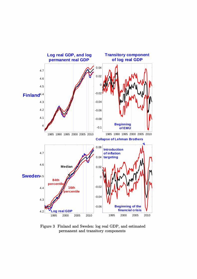
Figure 2 shows log real GDP, together with the median and the one-standard devia-

tion percentiles of the posterior distribution of its estimated permanent component,

for the U.S., the Euro area, and Japan, whereas the left-hand side column of Figure

3 shows the same objects for Finland and Sweden. Even the simple ‘eyeball metric’

clearly suggests that all severe financial crises considered herein have been character-

ized by a non-negligible negative impact on potential output dynamics, which in two

25Since one of our key results pertains to the impact of severe financial crises on potential out-

put dynamics, being able to effectively identify a permanent output shock is here of paramount

importance. This implies that, beyond output growth, inflation, and the short rate–which provide

a ‘minimal statistical summary’ of any economy, and should therefore be there–we need a fourth

variable with a strong informational content on the state of the business cycle.

16

cases–Japan, following the collapse of the asset prices bubble of the second half of

the 1980s, and Finland, in the early 1990s–appears to have been nothing short of

dramatic.

Figure 4 provides statistical evidence on this, by showing the posterior distrib-

utions of the difference between the annualized change in the estimated permanent

component of GDP from the temporary peak to the temporary trough associated

with the crisis,26 and the annualized change in the same object during the previous

five years.27 The only exception is Japan’s crisis of the early 1990s, for which we show

the posterior distribution of the difference between the annualized change in potential

output during the period following that crisis and up to the beginning of the most

recent crisis, and the annualized change in potential output during the entire period

before the first crisis. We do this in order to capture and characterize the obvious

decrease in the rate of growth of Japan’s potential output following the collapse of

the bubble of the second half of the 1980s. Finally, as for Sweden’s crisis of the first

half of the 1990s, the sample period is too short to allow us to make any comparison

between potential output dynamics before and during the crisis, and so we simply ig-

nore it. The visual evidence from the bottom-left panel of Figure 3, however, suggests

that, around the time of that crisis, potential output growth had been temporarily

depressed compared to the pace of growth potential output had exhibited during the

subsequent period, and up to the most recent crisis.

Overall, the evidence reported in Figure 4 paints a consistent picture, with all the

financial crises analyzed herein having systematically been associated with either a

temporary or–in the case of Japan’s crisis of the early 1990s–a permanent deteri-

oration in the evolution of potential output. Two things, in particular, ought to be

stressed about the evidence reported in the Figure.

First, statistical significance is very strong, with the fraction of draws from the

posterior distribution for which the impact of the financial crisis on potential output

dynamics is estimated to have been negative being greater than, or equal to 99 per cent

for all countries and all crises, with the single exception of the United States during

the most recent episode, for which ‘only’ 93.9 per cent of the draws are associated

with a temporary deterioration of potential output growth.

Second, the estimated magnitudes are definitely not negligible, with median esti-

mates of the impacts, in terms of the (temporary) change in the annualized growth

rate of potential output, ranging from -3.4 per cent for Sweden during the recent

26Temporary peaks and troughs in potential output have been identified based on the median

estimates of the permanent component of log real GDP. The dates of the peaks and troughs are

the following: for the United States, 2008Q3 and 2009Q1; for the Euro area, 2008Q1 and 2009Q1;

for Japan, 2008Q1 and 2009Q1 for the most recent recession, whereas for the previous episode we

compare the period from the beginning of the sample up to 1990Q4 and the period from 1991Q1 to

2007Q2; for Finland, 1990Q2 and 1993Q2 for the first crisis, and 2008Q1 and 2009Q3 for the most

recent; and for Sweden, 2008Q2 and 2009Q1.27We take, as a benchmark, the previous five years, rather than a longer period, in order to take

into account of the possibility of slow, secular changes in the rate of growth of potential output.

17

crisis, to a remarkable -6.2 per cent for Finland during the three years between the

potential output peak of 1990Q2 and its subsequent trough of 1993Q2, when (based

on median estimates) potential GDP decreased by 7.6 per cent.

The results shown in Figure 4 complement, and expand upon, RR’s findings on the

macroeconomic impact of financial crises. Not only, as they have documented, such

episodes have consistently been characterized by dramatic falls in actual output: our

findings point towards a similarly consistent and sizeable impact on potential output

dynamics. It is also to be stressed that these results are by no means incompatible

with PP’s (2011) finding, based on break tests applied within a univariate context,

that in most cases, following a financial crisis, output ultimately returns to the pre-

crisis trend. As PP point out, the average slump associated with such crises lasts

about nine years, so the fact that that the pre-crisis potential output trend reasserts

itself over such a long horizon is not incompatible with the notion that, at much

shorter horizons, potential output dynamics is negatively affected to a non-negligible

extent.

In the light of Athanasios Orphanides’ work on output gap mismeasurement, and

its role in inducing policy mistakes which contributed to igniting the U.S. Great Infla-

tion,28 our findings have an obvious policy relevance. To the extent that policymakers

interpreted the fall in actual output associated with financial crises as entirely due

to a decrease in the transitory component of output, they would over-estimate the

size of the output gap, and would therefore end up over-estimating the disinflationary

pressures in the economy.

3.1 Are financial crises special, or is it just the depth of the

recession?

Although a negative impact on potential output dynamics appears to have been a

feature common to all crises and all countries analyzed herein, this does not neces-

sarily imply that such a feature is specific to financial crises per se: an alternative,

plausible interpretation in indeed that such an impact is simply the consequence of

the extraordinary depth of the recessions associated with severe financial crises, so

that such contractions end up ‘blasting away pieces of the economy’, thus negatively

impacting potential output dynamics.

Prima facie evidence in favor of such a position is provided by the fact that,

during the recent crisis, both Japan and Sweden–neither of which has been at the

epicenter of the crisis, so that they have mostly been affected via trade channels, but

they have not experienced severe stresses in their banking systems–have nonethe-

less exhibited non-negligible, and highly statistically significant negative impacts on

potential output dynamics. The case of Sweden is, under this respect, especially in-

teresting, since (i) following the financial crisis of the early 1990s, its financial system

28See in particular Orphanides (2002), Orphanides (2003b), Orphanides (2001), and Orphanides

(2003a).

18

had been largely revamped and made significantly more resilient, and, most likely as

a result of this, (ii) as we write (July 25th, 2012) it has not exhibited, so far, any

problem comparable to those which have instead bedevilled (first and foremost) the

United States and the Euro area. By the same token, Finland–which belongs to

the Euro area, but, apart from having experienced a deep recession, it has been, so

far, only marginally affected by the financial crisis–has exhibited a dramatic and

highly statistically significant negative impact on potential output dynamics. The

experience of these three countries during the recent crisis therefore naturally sug-

gests that the negative impact on potential output dynamics we previously identified

has nothing to do with financial crises per se, and it rather likely originates from the

fact that–as extensively documented by RR (2009), such crises have been character-

ized by extremely deep recessions. Evidence for the United States is compatible with

this position. Before the recent crisis, the deepest post-WWII contraction had been

the Volcker recession, which had been characterized by a trough in annual real GDP

growth equal to -2.75 per cent (in 1982Q3), compared to the recent crisis’ trough of

-5.15 per cent in 2009Q2. And in fact, compatible with our conjecture, the Volcker

recession had indeed been characterized by a comparatively mild negative impact on

potential output dynamics. By the same token, the evidence reported in the second

panel of Figure 2 shows how, in the Euro area, the comparatively mild recession of

the first half of the 1990s was associated with a temporary deceleration in the rate of

growth of potential output, but no decrease in its level.

The main exception to the argument that financial crises are not special, in terms

of their negative impact on potential output dynamics, is provided by Japan’s crisis

of the early 1990s, which was associated with a sizeable decrease in trend output

growth, and is therefore, in a real sense, ‘in a league of its own’.

Let’s now turn to a discussion of the features which have been idiosyncratic to

individual crises.

4 Features Idiosyncratic to Individual Financial

Crises

4.1 A temporary increase in macroeconomic volatility

Figure 5 reports evidence on changes over time in macroeconomic volatility, by show-

ing the median and the one-standard deviation percentiles of the posterior distribu-

tions of the standard deviation of reduced-form innovations to the log-difference of

real GDP (in the top row), and of the log-determinant of Ω (in the bottom row),

which, following Cogley and Sargent (2002), we interpret as a measure of the VAR’s

‘total prediction variance’, that is, of the total amount of noise hitting the system at

each point in time.

For both the United States and the Euro area, the recent crisis has been charac-

19

terized by sizeable increases in both features.29 This is especially apparent for the

Euro area, where the standard deviation of reduced-form shocks to real GDP growth

has temporarily increased reaching (marginally) the highest value in the entire sample

period, whereas the VAR’s total prediction variance has interrupted the long-run sec-

ular decline it had been experiencing since the mid-1970s, returning, in the aftermath

of the collapse of Lehman Brothers, to values it took in the early 1990s.

The experience of the other three countries, however, shows that sizeable, tempo-

rary increases in macroeconomic volatility are not a robust common feature across

all financial crisis. First, for neither Japan, Finland, nor Sweden the financial crises

of the early 1990s were associated with any significant change in the standard de-

viations of reduced-form shocks to GDP growth. This is especially noteworthy for

Japan and Finland, which, during those years, experienced a dramatic deceleration

in potential output growth, and a prolonged and sizeable fall in the level of potential

output, respectively. Second, the evolution of the VAR’s total prediction variance is

even more intriguing: whereas Finland’s crisis of the early 1990s was characterized by

a temporary increase in the log-determinant of Ω, the corresponding crises in Japan

and Sweden were associated with no significant change, and a sizeable decrease, re-

spectively.

4.2 The persistence of output growth

By the same token, the evidence reported in Figure 6 shows that a temporary increase

in the persistence of real GDP growth–which, intuitively, we might be induced to

expect, in the light of RR’s finding about the length and depth of downturns associ-

ated with financial crises–has not been, in fact, a robust common feature of financial

crises. The top row shows the median and the one-standard deviation percentiles of

the posterior distribution of the fraction of variance of real GDP growth pertaining

to the frequency band [0, 16], which, at the quarterly frequency, is associated with

fluctuations with a frequency of oscillation slower than eight years. The bottom row

shows, for each quarter t, the fraction of draws from the posterior distribution for

which the fraction of variance of real GDP growth pertaining to the frequency band

[0, 16] in a quarter of reference30 is greater than it is in quarter t.31

29For either the U.S. or the Euro area, both the standard deviation of reduced-form innovations

to the log-difference of real GDP, and the log-determinant of Ω, clearly appear to have started

increasing well before the beginning of the crisis, in August 2007. The simplest and most logical

explanation for this result is that the estimates produced by the Gibbs sampler are, by construction,

two-sided, and in the case of processess experiencing sharp breaks they therefore tend to inevitably

smooth the break, thus ‘mixing the future with the past’, and giving the misleading impression that

the change took place before it actually did.30The quarters of reference are those corresponding to the maximum values taken by the medians

shown in the first row.31Evidence based on the normalized spectrum of output growth at =0 is very similar to that

shown in Figure 6. These results are not shown here for reasons of space, but they are available

20

Only for two countries severe financial crises clearly stand out, compared to stan-

dard business-cycle fluctuations, for being characterized by sizeable, temporary in-

creases in the persistence of output growth. The first is the United States, where,

during the recent crisis, the fraction of variance of real GDP growth pertaining to the

frequency band [0, 16] increased (based on median estimates) from 17 per cent in

2007Q2 to a peak of 36 per cent in the quarter following the collapse of Lehman Broth-

ers, 2008Q4. Since then it has been steadily decreasing, reaching about 22 per cent in

the last quarter of the sample. The fraction of draws for which the fraction of variance

of real GDP growth pertaining to the band [0, 16] in 2008Q4 is greater than in

quarter t paints a similar picture, falling from 84 per cent in 2007Q2 to slightly below

50% in 2009Q1, and then rebounding over subsequent quarters. The second country

is Sweden, where, during the crisis of the early 1990s, the fraction of variance of real

GDP growth associated with the low frequencies experienced a similar, but milder

temporary increase, and the fraction of draws, swiftly decreased from 78 per cent

in 1990Q4 to 50% in the quarter of reference, 1992Q4, and then quickly rebounded,

reaching 90 per cent in 1994Q1. This implies that these two episodes have been as-

sociated with deep and prolonged recessions not only because (trivially) they have

been characterized by comparatively large contractionary shocks, but also because–

conditional on those shocks–output growth has exhibited a systematic tendency to

revert to the mean more slowly than under normal circumstances.

For all other countries, on the other hand, evidence does not support the notion

that a temporary increase in the persistence of real GDP growth is a robust feature

of severe financial crises. For Japan, for example, the dramatic crisis of the early

1990s was not associated with any perceptible change in output growth persistence,

whereas the recent crisis has been characterized by a comparatively mild increase.

By the same token, Finland’s crisis of the early 1990s was not accompanied by any

significant change in output growth persistence. Evidence for the Euro area is more

complex. On the one hand, following the collapse of Lehman Brothers output growth

persistence appears indeed to have increased, although a proper interpretation of the

evidence is complicated by the fact that years immediately preceding the crisis had

been characterized by a decrease roughly of the same magnitude. The counterargu-

ment to the notion that a large increase in output growth persistence is a typical

feature of financial crises is provided by the recession of the early 1980s, which was

characterized by an extent of real GDP growth persistence just marginally lower than

the one associated to the recent crisis.

4.3 The role of individual structural disturbances

Let’s now turn to the role played by individual structural disturbances. The next two

sub-sections explore the specific sign pattern exhibited by such disturbances within

the context of individual financial crises, and the counterfactual paths the economy

from the author upon request.

21

would have travelled had individual shocks been absent.32

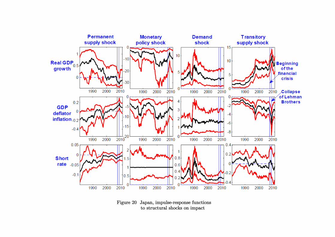
4.3.1 The sign pattern of structural shocks

Figures 7 to 9 show, for either country, and for either quarter, the fractions of draws

from the posterior distribution for which the four identified structural shocks are

estimated to have been positive.33 Within each panel, the red broken line represents

the average value taken by such a fraction over the entire sample period. The reason

for reporting this object is in order to be able to more precisely characterize to which

extent specific periods have been anomalous compared to the ‘normal’ pattern of

shocks’ signs for the entire sample period.34

Starting from the United States, the years immediately preceding the recent crisis

had been characterized by predominantly expansionary demand non-policy shocks,

and by predominantly contractionary supply shocks (either permanent or transitory),

and, marginally, by predominantly expansionary monetary policy shocks. Results for

the permanent supply shocks between the beginning of the century and the onset

of the financial crisis resonate with the well-known productivity slowdown which

took place during those years,35 whereas the weak evidence of expansionary mone-

tary policy shocks is incompatible, e.g., with John Taylor’s criticism of the Federal

Reserve’s monetary policy during those years,36 and is instead compatible with the

FED’s often-stated position that, in the run-up to crisis, its monetary policy had

not been especially expansionary.37 Particularly interesting is the reversal of the

sign pattern for the demand non-policy shocks, which are estimated to have been

most likely contractionary between the early 2000s and mid-2004, and most likely

expansionary between mid-2004 and the begining of the crisis. Since, as previously

32On the other hand, we eschew the issue of the volatility of individual structural shocks since, in

order to identify such volatilities, we would need to impose a set of normalizations on the impacts

of the shocks (see, e.g., Gambetti, Pappa, and Canova (2006))). Since any such normalization is

essentially arbitrary, we prefer to simply ignore the issue, rather than presenting results we would

regard as questionable.33It is to be noticed how such fractions fluctuate quite significantly over the interval [0, 1], with

the single exception of the permanent output shock. Intuitively, this is due to the fact that potential

output is estimated to have evolved very smoothly, so that the fraction of draws for which permanent

output shocks are estimated to have been positive has consistently remained close to one half.34Although such averages have almost uniformly been near-identical to 0.5, in a few instances

they have clearly been either slightly higher or slightly lower, thus suggesting that the corresponding

shocks have been, on average, either expansionary or contractionary. This has marginally been the

case for the potential output and monetary policy shocks for the Euro area, which are estimated to

have been, on average, mostly contractionary; and of the demand non-policy shocks for the U.S.,

Japan, and Sweden, which have been, instead, mostly expansionary.35E.g., the annual rate of growth of output per hour in the non-farm business sector decreased

from an average value of 3.6 per cent over the period 2000Q1-2004Q4, to an average value of 1.1 per

cent over the period 2005Q1-2007Q2.36See e.g. Taylor (2009).37 [Here put references: Bernanke’s speech at the AEA meetings, and the work of Kiley et al.]

22

discussed, credit market shocks should be expected to end up being classified, within

the present taxonomy, as demand non-policy shocks, this suggests that such shocks

played most likely an expansionary role in the run-up to the crisis. Since August

2007, on the other hand, the sign pattern has once again reversed, and, consistent

with what we would expect just based on (say) reading the financial press, it has

been most likely negative. Potential output shocks have been most likely negative

between the beginning of the crisis and 2009Q4, but over subsequent quarters the

sign pattern has most likely switched to positive.38 Finally, monetary policy shocks

have been most likely expansionary between mid-2007 and the collapse of Lehman

Brothers, but they have been most likely contractionary during subsequent quarters.

Interestingly, Gali, Smets, and Wouters (2012) obtain the same result based on an

estimated DSGE model, and interpret it as the logical consequence of the zero lower

bound having been binding during that period.

For other countries, the structural shocks’ sign patterns do not exhibit any con-

sistent similarity compared to the United States. For the Euro area, for example,

neither the monetary policy nor the demand non-policy shocks display any clear-cut

consistent sign pattern during the recent crisis, whereas, in line with the discussion of

Section 3, the negative impact on potential output dynamics is largely concentrated

in the quarters between the beginning of the crisis and the collapse of Lehman Broth-

ers. Consistent with the U.S.’ recent crisis, Japan’s crisis of the early 1990s had been

characterized by most likely expansionary demand non-policy shocks in the run-up

to the crisis, and by most likely contractionary shocks over the subsequent period.

Monetary policy shocks had been most likely expansionary around the mid-1990s

and in the run-up to the recent crisis, but other than that they have not exhibited

any clear-cut sign pattern. Likewise, transitory supply shocks have been most likely

expansionary in the run-up to both crises, but again, other than that, they have not

displayed any consistent pattern. Finally, given the dramatic slowdown in Japan’s

potential output growth starting in the early 1990s, the lack of any consistent sign

pattern in permanent output shocks over the entire sample period may appear, at

first sight, as puzzling. It is important to stress, however, that given the permanent

nature of the slowdown in real GDP growth, the time-varying VAR has captured it

by means of a permanent decrease in the VAR-generated unconditional mean for the

log-difference of GDP. To put it differently, since the slowdown in output growth has

been permanent, the VAR has ‘allocated’ it its time-varying unconditional mean vec-

tor, rather than to the permanent output shocks. Turning to Finland and Sweden’s

crises of the early 1990s, the pattern for demand non-policy shocks is in line with

that for Japan’s crisis during the same period, and for the United States during the

recent crisis: for Finland, shocks had been most likely positive in the run-up to the

crisis, and negative therefore; for Sweden, on the other hand, we can’t say anything

about the run-up to the crisis, which was before the start of the sample period, but

38Once again, this resonates with the evolution of the rate of growth of output per hour in the

non-farm business sector, which, likewise, exhibited a dramatic peak in 2009Q4.

23

following the outbreak of the crisis shocks had most likely been negative. For both

countries, monetary policy shocks are were most likely positive during the quarters

immediately following the outbreak of that crisis, whereas potential output shocks

had been most likely negative for Finland, but, quite strikingly, most likely positive

for Sweden. Finally, during the recent crisis, the most clear-cut sign pattern per-

tains potential output shocks in Finland, and, to a slightly lesser extent, in Sweden,

which, as expected, have been almost uniformly negative, whereas other shocks do

not exhobit any clear pattern.

Overall, the sign pattern of structural shocks in the run-up to, and during financial

crises has no exhibited any clear-cut consistent behavior. It is to be noticed, however,

that in most cases–with the most notable exception being the Euro area during the

recent crisis–demand non-policy shocks, which should here be expected to capture

credit market disturbances, did indeed display a consistent pattern, expansionary in

the run-up to the crisis, and contractionary following its outbreak. So, although,

strictly speaking, our results do not point towards a universal, consistent pattern for

structural shocks’ signs, for demand non-policy shocks we come quite close to that.

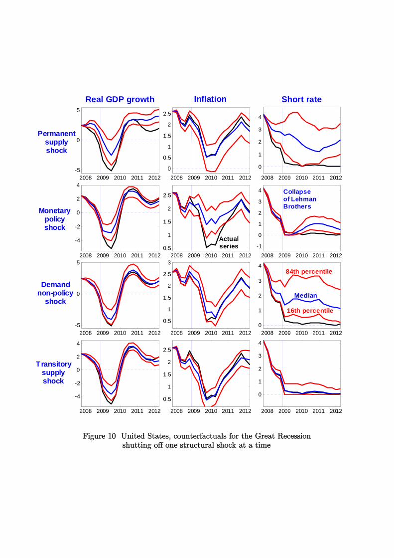
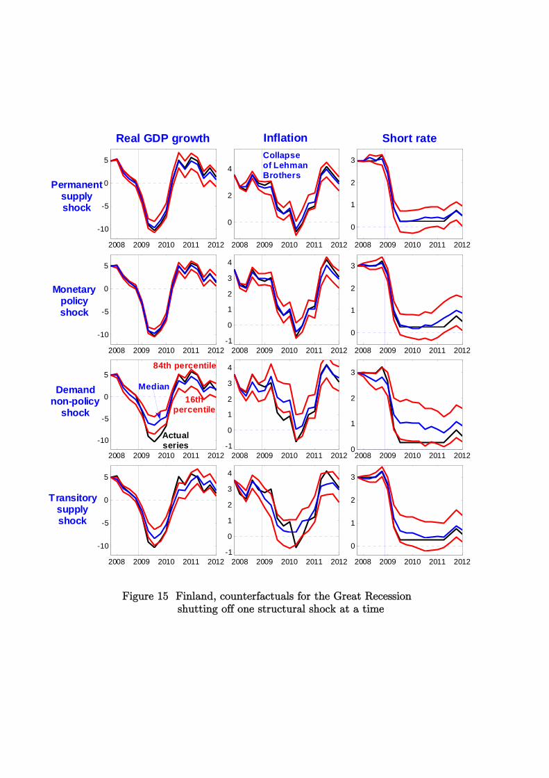
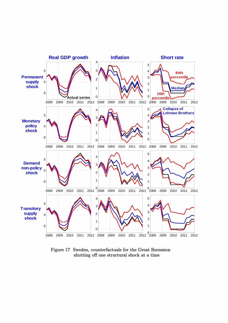
4.3.2 Counterfactuals shutting off individual structural shocks39

An alternative way of assessing the role played by individual structural disturbances

is to explore what the time path of the endogenous variables would have been had

one of those disturbances been absent. Figure 10 to 17 provide evidence on this,

by showing, for each country, and for all the financial crises considered herein, the

actual paths of annual real GDP growth, annual inflation, and the short rate, together

with the median and the 16th and 84th percentiles of the posterior distributions of the

counterfactual paths obtained by setting to zero one structural shock at a time.40 For

reasons of space, in what follows I will mostly discuss results for real GDP growth, and

I will only mention results for other variables when I deem them to be of particular

interest.

Starting from the United States, the results shown in the first column of Figure

10 highlight how, within the context of the recent crisis, all shocks have played an

overall contractionary role, as setting to zero either of them systematically generates a

higher counterfactual path for real GDP growth. At the same time, it is apparent how

39For reasons of space we do not discuss results for the fractions of forecast error variance of

individual series at the various horizons attributable to individual structural disturbances. Unsur-

prisingly, these results are, conceptually, essentially the same as those discussed in this sub.section.

All of these additional results are available from the author upon request.40So, to be clear, each counterfactual has been computed by taking as given the evolution of the

log-differences of real GDP and the GDP deflator, of the short rate, and of either the unemployment

rate or the consumption-output ratio up to a quarter -1. Then, starting from quarter , marking

the beginning of the financial crisis of interest, we ‘re-run history’ by setting to zero one structural

shock at a time. As for the recent crisis, is set to 2007Q3 for all countries. As for the financial

crises of the early 1990s, on the other hand, is set to 1989Q4 for Finland and Japan, and to 1991Q4

for Sweden.

24

setting to zero demand non-policy shocks only produces a slightly higher counterfac-

tual path–thus pointing towards a comparatively limited role played by such shocks

within the context of the recen crisis–whereas, by the same token, the role played

by transitory supply shocks has been only marginally more important. On the other

hand, evidence suggests that permanent output shocks and monetary policy shocks

have played a dominant, and roughly equal role, with the counterfactual paths for real

GDP growth being significantly higher than the actual, historical path. Consistent

with the discussion of the previous sub-section, the fact that ‘killing off’ monetary

policy shocks generates a higher counterfactual path for real GDP growth derives

from the fact that, within the context of the Great Recession, the zero lower bound

has been binding. In turn, this implies that, for the most recent period, the struc-

tural VAR necessarily ends up estimating positive monetary policy shocks, so that,

setting them to zero in the counterfactual, automatically produces a higher paths for

output growth. Interestingly, as far as inflation is concerned the only counterfactual

to produce materially different results–specifically, a higher inflation path–is the

one in which the monetary policy shock is set to zero.

Turning to the Euro area, the key finding emerging from Figure 11 is the dominant

role played by the permanent output shock within the context of the recent crisis.

Whereas setting to zero either of the other three shocks produces counterfactual paths

for the three series of interest which are only marginally different from the actual,

historical paths, killing off the permanent output shock generates significantly higher

counterfactual paths for all series. In particular, based on median estimates real GDP

growth would have experienced a trough equal to -2.3 per cent in 2009Q2, as opposed

to an actual trough of -5.5 per cent in the previous quaretr, whereas inflation would

have experienced a modest fall, with a counterfactual trough equal to 1.5 per cent,

compared to the actual trough of 0.3 per cent. As a result of this, the short rate

would have remained systematically higher, and instead of rapidly falling towards,

and then remaining close to zero following the collapse of Lehman Brothers, it would

have reached a trough of 2.1 per cent in 2010Q2, and it would have then edged slightly

upwards over subsequent quarters.

In spite of the dramatic deceleration in real GDP growth following Japan’s crisis

of the early 1990s, killing off permanent output shocks would have produced an only

marginally higher counterfactual path for output growth. This originates from the

fact that, as we pointed out in the previous sub-section, the permanent decrease in

output growth has been captured by the VAR by means of a permanent decrease

in the VAR-implied time-varying mean for this series, thus automatically minimizing

the role played by permanent output shocks. By the same token, setting to zero either

of the other shocks would have produced the same result. As for the recent crisis, the

most interesting result is that, in spite of the previously discussed temporary decrease

in potential output associated with the crisis, killing off permanent output shocks does

not produce a huge increase in real GDP growth. This originates from the fact that,

as it is apparent from Figure 2, the peak-to-trough decrease in actual output during

25

the crisis was significantly larger than the corresponding peak-to-trough decrease in

potential output, which implies that, different from the Euro area, transitory output

shocks played a dominant role. As the remaining three panels of the first column of

Figure 13 show, in fact the key role was played by transitory supply shocks, whereas

the two demand-side shocks’ role has been essentially negligible.

Permanent output shocks played on the contrary a dominant, and dramatic role

within the context of Finland’s crisis of the early 1990s. Consistent with the potential

output estimates reported in Figure 3, killing off such shocks would have generated

a significantly higher counterfactual path for output growth. In particular, based on

median estimates, first, real GDP growth would have reached a trough of -3.9 per

cent in 1991Q1, as opposed to the actual trough of -7.1 per cent in 1991Q4. Second,

the median counterfactual path for output growth is so much higher than the actual

one that the recession would have ended (that is: GDP growth would have turned

positive) in 1992Q2, five quarters before it actually did. By contrast, the counter-

factual paths for output growth obtained by setting to zero either of the other three

shocks are only marginally different from the actual one. Whereas the counterfactual

paths for inflation are only slightly different from the actual path–with the possible

exception of the one obtained by killing off demand non-policy shocks–those for the

short rate exhibit two interesting results. First, absent permanent output shocks, the

short rate would have been uniformly lower, thus reflecting a policy, on the part of

Finland’s monetary authority, of accomodating benign permanent supply shocks.41

Second, by the same token, eliminating demand non-policy shocks generates a higher

counterfactual path for the short rate, reflecting the standard reaction, on the part of

central banks, to the previously discussed series of negative demand shocks (see the

the third panel of the second row of Figure 8).

Finally, Figure 16 shows how Sweden’s recession of the early 1990s was due to a

combination of al shocks, with a dominant role of permanent output shocks, and a

negligible role for demand non-policy shocks. The same holds true for the most recent

crisis, with, again, a dominant role of permanent output shocks, and a negligible role

played instead by monetary policy shocks.

4.4 Impulse-response functions to structural innovations

Figures 18 to 22 show the normalized IRFs42 on impact of real GDP growth, inflation,

and the short rate to each of the four identified structural shocks.43 The IRFs to

a permanent output shock are normalized so that, for each single IRF, the long-

41This is conceptually in line with, e.g., the Federal Reserve’s accomodation, under Alan

Greenspan, of the productivity acceleration of the second half of the 1990s, by keeping the Fed-

eral Finds rate comparatively low.42We compute the IRFs via the Monte Carlo integration procedure described in Appendix C, which

allows us to tackle the uncertainty originating from future time-variation in the VAR’s structure.43For reasons of space we only show IRFs on impact, but the full set of results for IRFs at horizons

up to five years after the impact are available upon request.

26

run impact of log real GDP is equal to one, whereas those for the monetary policy

shock have been normalized so that, for each quarter, the median of the posterior

distribution of the impact on the short rate at zero is equal to one (which is apparent

from the bottom panel of the second column of either figure). Since for neither of the

other two shocks there exists such a natural normalization, we have normalized them

by setting, for each quarter, the median of the posterior distribution of the impact

at zero on the cyclical variable (either the unemployment rate, or the consumption-

output ratio) equal to one. Once again, for reasons of space in what follows we are

going to focus on the IRFs for real GDP growth, and we are going to discuss those

for the other two series only when they exhibit especially interesting features.

Starting from the United States, the key feature emerging from Figure 18 is the

absence of any clear-cut peculiarity of the recent financial crisis compared to the rest

of the sample period. For example, although the impact of a permanent output shock

on real GDP growth at zero appears to have fallen compared to the years immediately

preceding the crisis, such a decrease is well within the bounds of historical variation

exhibited between the mid-1960s and the onset of the financial crisis. The same

holds true for the Euro area: although, following August 2007, the impact on GDP

growth of a permanent output shock appears to have slightly increased, the extent

of variation is nowhere near that experienced during the decade of the 1980s. For

the Euro area, too, it is not possible to identify any obvious peculiarity of the recent

crisis, compared to the rest of the sample period, for any variable and any shock.

Turning to Japan, the crisis of the early 1990s was marked by a sizeable decrease

of the impact of permanent output shocks on GDP growth at zero, and by a corre-

sponding increase of the impact of transitory supply shocks. By the same token, the

reaction of the short rate to demand non-policy shocks exhibited a large, temporary

increase around the time of the crisis, likely reflecting the more aggressive monetary

policy stance adopted by the Bank of Japan in its attempt to forestall the negative

headwinds generated by a series of negative demand shocks (see the third panel of

the first row of Figure 8). This finding gains additional relevance in the light of

the analogous temporary increase in the impact of such shocks on real GDP growth.

Overall, our results paint therefore a picture in which the impact of demand shocks

(normalized on the consumption-output ratio) temporarily increased during the cri-

sis, thus spurring the central bank to increase, likewise, the strength of its reaction

to such shocks. As for the recent crisis evidence is weaker, and it suggests that the

impact of supply-side shocks, both permanent and transitory, has been qualitatively

the same as during the same as, but milder than during the previous crisis.

As for Finland, the crisis of the early 1990s does not exhibit any clear-cut peculiar

feature. The impact of demand non-policy shocks on real GDP growth, for example,

would appear to have increased around the time of te crisis, but once again, such

an increase is well within the bounds of normal, secular variation in the rest of the

sample. As for the recent crisis, the most notable features are (i) a decrease in the

impact on GDP growth of permanent output shocks; (ii) temporary increases in the

27

magnitude of the impacts of transitory supply shocks on either variable; and (iii)

sizeable temporary increases of the impact of demand non-policy shocks on output

growth and the short rate, with peaks corresponding to the quarter of the collapse

of Lehman Brothers. An important point to stress, however, is that since Finland

has been, since January 1999, part of the Euro area, the reaction of the short rate to

structural shocks specific to Finland–which the VAR just produces ‘mechanically’–

does not have a straighforward interpretation, especially in the light of the fact that

Finland represents, in terms of GDP, a very small fraction of the entire Euro area, so

that the European Central bank’s monetary policy reacts to Finland-specific shocks to

a very limted extent. On the other hand, it is important to keep in mind that, within

the context of the recent crisis, structural shocks should logically be expected to have

been very strongly synchronized across Euro area countries, which implies that the

evidebnce reported in the bottom row of Figure 21 is not, in fact, meaningless, and

it rather difficult to interpret.

Finally, as for Sweden, evidence does not point towards obviously distinctive fea-

tures associated to financial crises, with the exception of a sizeable decrease in the

magnitude of the impact of transitory supply shocks on inflation during the crisis

of the early 1990s, and of the impact of supply-side shocks, both permanent and

transitory, on GDP growth during the most recent one.

5 Conclusions

In this paper we have used Bayesian time-varying parameters structural VARs with

stochastic volatility to investigate the specific dimensions along which recessions asso-

ciated with severe financial crises have historically been different from ‘normal’ reces-

sions, and standard business-cycle fluctuations, in the post-WWII U.S., Japan, Euro

area, Sweden, and Finland. We have identified four structural shocks by combining

a single long-run restriction, to identify a permanent output shock as in Blanchard

and Quah (1989), with three sign restrictions to identify demand- and supply-side

transitory shocks.

Evidence suggests that severe financial crises have systematically been character-

ized by a negative impact on potential output dynamics, which in two cases–Japan,

following the collapse of the asset prices bubble of the second half of the 1980s, and

Finland, in the early 1990s–appears to have been nothing short of dramatic. On

the other hand, with very few exceptions, neither the relative importance of the dif-

ferent types of shocks, the way they have been propagating through the economy,

the persistence of output growth, or the fractions of forecast error variance explained

by individual shocks have exhibited any systematic difference compared to standard

macroeconomic fluctuations. Our main conclusion is therefore that, once controlling

for the size of the shocks, financial crises appear to have been broadly similar to

standard macroeconomic fluctuations along most, but not all, dimensions.

28

A The Data

Here follows a detailed description of the dataset.

A.1 United States

Quarterly seasonally adjusted series for real GDP (‘GDPC96: Real Gross Domestic

Product, 3 Decimal, Seasonally Adjusted Annual Rate, Billions of Chained 2005 Dol-

lars’) and the GDP deflator (‘GDPCTPI: Gross Domestic Product: Chain-type Price

Index, Seasonally Adjusted’) are from the U.S. Department of Commerce: Bureau of

Economic Analysis. A monthly seasonally adjusted series for the civilian unemploy-

ment rate (‘UNRATE: Civilian Unemployment Rate, Seasonally Adjusted, Percent’)

is from the U.S. the Department of Labor: Bureau of Labor Statistics, and it has

been converted to the quarterly frequency by taking averages within the quarter. A

monthly seasonally adjusted series for the 3-month Treasury Bill (‘TB3MS: 3-Month

Treasury Bill: Secondary Market Rate’) is from Board of Governors of the Federal

Reserve System, and it has been converted to the quarterly frequency by taking av-

erages within the quarter. The quarterly series for potential GDP (‘GDPPOT: Real

Potential Gross Domestic Product, Quarterly, Billions of Chained 2005 Dollars’) is

from the U.S. Congressional Budget Office, Budget and Economic Outlook.

A.2 Euro area

Quarterly, seasonally adjusted series for real GDP, the GDP deflator, and real con-

sumption expenditure are from the European Central Bank’s database. For all series,

the sample period is 1963Q1-2012Q1. A monthly series for a short rate, available for

the period January 1970-December 2011, is from the European Central Bank’s data-

base, and it has been converted to the quarterly frequency by taking averages within

the quarter. The series has been extended backwards in time to 1963Q1 by linking

it to a weighted average of short rates for nine Euro area countries, with weight set

to 0.3 for Germany, 0.2 for both France and Italy, and to 0.05 for the remaining six

countries. Since the first ten years of data (that is, 1963Q2 to 1973Q2) are used to

compute the (comparatively loose) priors, the fact that, up to 1969Q4, we rely on a

reasonable proxy for the authentic, unavailable synthetic Euro area short rate is to

be regarded, in our own view, as entirely legitimate.

A.3 Japan

Quarterly, seasonally adjusted series for real GDP, the GDP deflator, and real con-

sumption expenditure are from the OECD’s Quarterly National Accounts, and are

available for the period 1980Q1-2011Q4 (their acronyms are QNA.Q.JPN.CMPGDP.

VIXOBSA.2000_S1, QNA.Q.JPN.CMPGDP.DOBSA.2000_S1, andOT.Q. JPN. CMPPC.

VIXOBSA.2000. S1.VAL respectively). A monthly series for a short rate (‘Official

29

discount rate, rate for commercial bills discounted by financial institutions for loans

secured by the government’) is from the Bank for International Settlements database,

and is available for the period April 1955-December 2011.

A.4 Sweden

Quarterly, seasonally adjusted series for real GDP, the GDP deflator, nominal GDP,

and nominal private final consumption expenditure are from the International Mon-

etary Fund’s International Financial Statistics. The series for real GDP is available

for the period 1970Q1-2011Q4, whereas the other three series are available for the

period period 1980Q1-2011Q4. The consumption-output ratio has been computed as

the ratio between nominal consumption expenditure and nominal GDP. A monthly

series for a short rate (‘Interest Rates, Discount Rate, Percent per Annum’) is from

the International Monetary Fund’s International Financial Statistics, and is available

for the period January 1960-December 2011.

A.5 Finland

Quarterly, seasonally adjusted series for real GDP, the GDP deflator, nominal GDP,

and nominal private final consumption expenditure are from the International Mon-

etary Fund’s International Financial Statistics, and are all available for the period

1970Q1-2011Q4. The consumption-output ratio has been computed as the ratio be-

tween nominal consumption expenditure and nominal GDP. A monthly series for a

short rate (‘Interest Rates, Discount Rate, Percent per Annum’) is from the Inter-

national Monetary Fund’s International Financial Statistics, and is available for the

period January 1960-December 2011.

B Details of the Markov-Chain Monte Carlo Pro-

cedure

We estimate (1)-(8) via Bayesian methods. The next two subsections describe our

choices for the priors, and the Markov-Chain Monte Carlo algorithm we use to sim-

ulate the posterior distribution of the hyperparameters and the states conditional

on the data, while the third section discusses how we check for convergence of the

Markov chain to the ergodic distribution.

B.1 Priors

For the sake of simplicity, the prior distributions for the initial values of the states–

0 and 0–which we postulate all to be normal, are assumed to be independent

both from each other, and from the distribution of the hyperparameters. In order to

30

calibrate the prior distributions for 0 and 0 we estimate a time-invariant version of

(1) based on the first 10 years of data, and we set

0 ∼ h 4 · ()

i(B1)

where () is the estimated asymptotic variance of . As for 0, we proceed

as follows. Let Σ be the estimated covariance matrix of from the time-invariant

VAR, and let be its lower-triangular Cholesky factor–i.e., 0 = Σ. We set

ln0 ∼ (ln0 10× ) (B2)

where 0 is a vector collecting the logarithms of the squared elements on the diagonal

of . As stressed by Cogley and Sargent (2005), ‘a variance of 10 is huge on a

natural-log scale, making this weakly informative’ for 0.

Turning to the hyperparameters, we postulate independence between the parame-

ters corresponding to the two matrices and –an assumption we adopt uniquely

for reasons of convenience–and we make the following, standard assumptions. The

matrix is postulated to follow an inverted Wishart distribution,

∼ ¡−1 0

¢(B3)

with prior degrees of freedom 0 and scale matrix 0. In order to minimize the

impact of the prior, thus maximizing the influence of sample information, we set

0 equal to the minimum value allowed, the length of plus one. As for , we

calibrate it as = × Σ, setting =1.0×10−4, the same value used in Cogley andSargent (2005), and a slightly more ‘conservative’ prior (in the sense of allowing for

less random-walk drift) than the 3.5×10−4 used by Cogley and Sargent (2005). Asfor , we postulate it to be normally distributed with a ‘large’ variance,

() = (0, 10000·(−1)2) (B4)

Finally, as for the variances of the stochastic volatility innovations, we follow Cogley

and Sargent (2002, 2005) and we postulate an inverse-Gamma distribution for 2 ≡Var():

2 ∼

µ10−4

21

2

¶(B5)

B.2 Simulating the posterior distribution

We simulate the posterior distribution of the hyperparameters and the states con-

ditional on the data via the following MCMC algorithm, as found in Cogley and

Sargent (2005). In what follows, denotes the entire history of the vector up to

time –i.e. ≡ [01, 02, , 0]0–while is the sample length.

31

(a) Drawing the elements of Conditional on , , and , the observation

equation (1) is linear, with Gaussian innovations and a known covariance matrix.

Following Carter and Kohn (2004), the density ( | ) can be factored as

( | ) = ( | )

−1Y=1

(|+1 ) (B6)

Conditional on and , the standard Kalman filter recursions nail down the first

element on the right hand side of (A6), ( | ) = ( ), with being

the precision matrix of produced by the Kalman filter. The remaining elements in

the factorization can then be computed via the backward recursion algorithm found,

e.g., in Kim and Nelson (2000), or Cogley and Sargent (2005, appendix B.2.1). Given

the conditional normality of , we have

|+1 = | + |−1+1| (+1 − ) (B7)

|+1 = | − |−1+1|| (B8)

which provides, for each from -1 to 1, the remaining elements in (1), (|+1, ,

, ) = (|+1, |+1). Specifically, the backward recursion starts with a drawfrom ( ), call it Conditional on , (A7)-(A8) give us −1| and −1| ,thus allowing us to draw −1 from (−1| −1| ), and so on until =1.(b) Drawing the elements of Conditional on

, , and , the orthogonalised

innovations ≡ (-0), with Var()=, are observable. Following Cogley and

Sargent (2002), we then sample the ’s by applying the univariate algorithm of

Jacquier, Polson, and Rossi (1994) element by element.44

(c) Drawing the hyperparameters Conditional on , , , and , the innova-

tions to and to the ’s are observable, which allows us to draw the hyperparameters–

the elements of and the 2–from their respective distributions.

(d) Drawing the elements of Finally, conditional on and the ’s are

observable, satisfying

= (B9)

with the being a vector of orthogonalized residuals with known time-variying vari-

ance . Following Cogley and Sargent (2005), we interpret (B9) as a system of

unrelated regressions. The first equation in the system is given by 1 ≡ 1, while

the following equations can be expressed as transformed regressions as³− 12

2 2

´= −21

³−12

2 1

´+³− 12

2 2

´(B10)³

− 12

3 3

´= −31

³−12

3 1

´− 32

³− 12

3 2

´+³−12

3 3

´44For details, see Cogley and Sargent (2005, Appendix B.2.5).

32

³− 12

(−1)2(−1)2´= −(−1)21

³− 12

(−1)21´−

− (−1)2(−1)2³− 12

(−1)2(−1)2´+³−12

(−1)2(−1)2´

where the residuals are independent standard normal. Assuming normal priors for

each equation’s regression coefficients the posterior is also normal, and can be com-

puted via equations (77) of (78) in Cogley and Sargent (2005, section B.2.4).

Summing up, the MCMC algorithm simulates the posterior distribution of the

states and the hyperparameters, conditional on the data, by iterating on (a)-(d). In

what follows, we use a burn-in period of 50,000 iterations to converge to the ergodic

distribution, and after that we run 10,000 more iterations sampling every 10th draw

in order to reduce the autocorrelation across draws.45

C Computing Generalised Impulse-Response Func-

tions

Here we describe the Monte Carlo integration procedure we use in Section 4.4 in order

to compute the generalised IRFs to the structural shocks.

Randomly draw the current state of the economy at time from the Gibbs sam-

pler’s output. Given the current state of the economy, repeat the following procedure

100 times.

• Draw four independent (0, 1) variates (the four structural shocks), and basedon the relationship = 0, with ≡ [ , ,

,

]

0–where ,

, , and are the permanent output shock, and the interest rate, de-

mand non-interest rate, and transitory supply structural shocks, respectively–

compute the reduced-form shocks at time .

• Simulate both the VAR’s time-varying parameters and the covariance matrixof its reduced-form innovations, Ω, 40 quarters into the future. Based on the

simulated Ω, randomly draw reduced-form shocks from +1 to +40. Based

on the simulated , and on the sequence of reduced-form shocks from to

+40, compute simulated paths for the four endogenous variables. Call these

simulated paths as

+40, with = 1, .., 100.

• Repeat the same procedure based on exactly the same simulated paths for theVAR’s time-varying parameters, the ; the same reduced-form shocks at times

+1 to +40; and the same structural shocks , , , and at time ,

with the only difference that, in order to compute the GIRF to shock , with

45In this we follow Cogley and Sargent (2005). As stressed by Cogley and Sargent (2005), however,

this has the drawback of ‘increasing the variance of ensemble averages from the simulation’.

33

= , , , , you set = 1. Call these simulated paths as

+40, with

= 1, .., 100.

For each of the 100 iterations define

+40 ≡

+40−

+40. Finally, compute

each of the 1,000 generalised IRFs as the mean of the distribution of the

+40’s.

34

References

Benati, L. (2008): “The Great Moderation in the United Kingdom,” Journal ofMoney, Credit, and Banking, 39(1), 121—147.

Benati, L., and C. Goodhart (2011): “Monetary Policy Regimes and EconomicPerformance: The Historical Record, 1979-2008,” in B. Friedman, B., and Wood-

ford, M. (eds.), Handbook of Monetary Economics, Volume 3, North Holland.

Benati, L., and T. Lubik (2012): “Sales, Inventories, and Real Interest Rates:A Century of Stylized Facts,” University of Bern and Federal Reserve Bank of

Richmond, mimeo.

Blanchard, O. J., and D. Quah (1989): “The Dynamic Effects of AggregateDemand and Supply Disturbances„” American Economic Review, 79(4), 655—673.

Bordo, M. D., and J. G. Haubrich (2011): “Deep Recessions, Fast Recoveries,and Financial Crises: Evidence from the American Record,” Rutgers University

and Federal Reserve Bank of Cleveland, mimeo.

Canova, F., and M. Paustian (2011): “Measurement with Some Theory: Us-ing Sign Restrictions to Evaluate Business Cycle Models,” Journal of Monetary

Economics, 58, 345—361.

Carter, C. K., and R. P. Kohn (2004): “On Gibbs Sampling for State SpaceModels„” Biometrika, 81, 541—553.

Cerra, V., and S. C. Saxena (2008): “Growth Dynamics: The Myth of EconomicRecovery,” American Economic Review, 98(1), 439—457.

Cochrane, J. H. (1994): “Permanent and Transitory Components of GNP andStock Prices,” Quarterly Journal of Economics, 109(1), 241—265.

Cogley, T. (2005): “How Fast Can the New Economy Grow?,” Journal of Macro-economics, 27(2), 179—207.

Cogley, T., and T. J. Sargent (2002): “Evolving Post-WWII U.S. InflationDynamics,” in B. Bernanke and K. Rogoff, eds. (2002), NBER Macroeconomics

Annuals 2001.

(2005): “Drifts and Volatilities: Monetary Policies and Outcomes in the

Post WWII U.S.,” Review of Economic Dynamics, 8(April), 262—302.

Cogley, T. W. (1990): “International Evidence on the Size of the Random-Walkin GNP,” Journal of Political Economy.

35

DelNegro, M. (2003): “Discussion of Cogley and SargentŠs ’Drifts and Volatilities:Monetary Policy and Outcomes in the Post WWII U.S.’,” Federal Reserve Bank of

Atlanta, Working Paper 2003-26.

Fry, R., and A. Pagan (2007): “Some Issues in Using Sign Restrictions for Iden-tifying Structural VARs,” NCER Working Paper n. 14, April 2007.

Gali, J., and L. Gambetti (2009): “On the Sources of the Great Moderation,”American Economic Journal: Macroeconomics, 1(1), 26—57.

Gali, J., F. Smets, and R. Wouters (2012): “Slow Recoveries: A Structural

Investigation,” Journal of Money, Credit, and Banking, forthcoming.

Gambetti, L., E. Pappa, and F. Canova (2006): “The Structural Dynamicsof U.S. Output and Inflation: What Explains the Changes?,” Journal of Money,

Credit, and Banking, 40(2-3), 369—388.

Golub, G., and C. VanLoan (1996): Matrix Computations, III Edition. JohnsHopkins University Press, Baltimore.

Jacquier, E., N. G. Polson, and P. Rossi (1994): “Bayesian Analysis of Stochas-tic Volatility Models„” Journal of Business and Economic Statistic, 12, 371—418.

Kim, C. J., and C. Nelson (2000): State-Space Models with Regime Switching.Cambridge, Mass., The MIT Press.

Lopez-Salido, D., and E. Nelson (2010): “Postwar Financial Crises and Eco-nomic Recoveries in the United States,” Federal Reserve Board, mimeo.

Orphanides, A. (2001): “Monetary Policy Rules Based on Real-Time Data,” Amer-ican Economic Review, 91(4), 964—985.

Orphanides, A. (2002): “Monetary Policy Rules and the Great Inflation,” Ameri-can Economic Review, 92(May 2002), 115—120.

Orphanides, A. (2003a): “Historical Monetary Policy Analysis and the TaylorRule,” Journal of Monetary Economics, 50, 983—1022.

(2003b): “The Quest for Prosperity Without Inflation,” Journal of Monetary

Economics, 50(April 2003), 633—663.

Papell, D. H., and R. Prodan (2011): “The Statistical Behaviour of GDP Fol-lowing Financial Crises and Severe Recessions,” University of Houston, mimeo.

Primiceri, G. E. (2005): “Time Varying Structural Vector Autoregressions andMonetary Policy,” The Review of Economic Studies, 72, 821—852.

36

Reinhart, C., and K. Rogoff (2009): This Time Is Different. Princeton Univer-sity Press.

Rubio-Ramirez, J., D. Waggoner, and T. Zha (2005): “Structural Vector Au-toregressions: Theory of Identification and Algorithms for Inference,” Review of

Economic Studies, 77(2), 665U—696.

Stock, J. H., and M. W. Watson (2012): “Disentangling the Channels of the2007-2009 Recession,” Brookings Papers on Economic Activity, forthcoming.

Taylor, J. B. (2009): Getting Off Track. Hoover Institution Press.

37

Figure 1 United States, Euro area, and Japan: estimated transitory components of log real GDP

Figure 2 United States, Euro area, and Japan: log real GDP and estimated permanent component

30

1985 1990 1995 2000 2005 2010

4

4.1

4.2

4.3

4.4

4.5

4.6

4.7

Log real GDP, and logpermanent real GDP

1985 1990 1995 2000 2005 2010

-0.1

-0.08

-0.06

-0.04

-0.02

0

0.02

0.04

Transitory componentof log real GDP

1995 2000 2005 20104.2

4.3

4.4

4.5

4.6

4.7

1995 2000 2005 2010

-0.06

-0.04

-0.02

0

0.02

0.04

0.06Introductionof inflationtargeting

Collapse of Lehman Brothers

Sweden

Log real GDP

Median

Beginning of thefinancial crisis

16thpercentile

84thpercentile

Finland

Beginningof EMU

Figure 3 Finland and Sweden: log real GDP, and estimated

permanent and transitory components

Figure 4 Financial crises and potential output dynamics: posterior distribution of the difference between the annualized peak-to-trough change in potential output during the crisis, and its annualized change during the previous five years (for Japan’s early 1990s crisis, the comparison is between the periods before and after the crisis)

Figure 5 Standard deviation of reduced-form innovations to the log-difference of real GDP, and log-determinant of Ωt

Figure 6 Output growth persistence

35

Figure 7 United States and Euro area: fractions of draws for which the structural shocks have been positive

36

Figure 8 Japan and Finland: fractions of draws for which the structural shocks have been positive

37

Figure 9 Sweden: fractions of draws for which the structural shocks have been positive

31

2008 2009 2010 2011 2012-5

0

5

Real GDP growth

2008 2009 2010 2011 2012

0

0.5

1

1.5

2

2.5

Inflation

2008 2009 2010 2011 2012

0

1

2

3

4

Short rate

2008 2009 2010 2011 2012

-4

-2

0

2

4

2008 2009 2010 2011 20120.5

1

1.5

2

2.5

2008 2009 2010 2011 2012

-1

0

1

2

3

4

2008 2009 2010 2011 2012-5

0

5

2008 2009 2010 2011 2012

0.5

1

1.5

2

2.5

3

2008 2009 2010 2011 20120

1

2

3

4

2008 2009 2010 2011 2012

-4

-2

0

2

4

2008 2009 2010 2011 2012

0.5

1

1.5

2

2.5

2008 2009 2010 2011 2012

0

1

2

3

4

Demandnon-policy

shock

Monetarypolicyshock

Permanentsupplyshock

Transitorysupplyshock

Collapseof LehmanBrothers

16th percentile

Median

84th percentile

Actualseries

Figure 10 United States, counterfactuals for the Great Recession shutting off one structural shock at a time

32

2008 2009 2010 2011 20120

1

2

3

Inflation

2008 2009 2010 2011 20120

1

2

3

4

5

Short rate

2008 2009 2010 2011 2012-6

-4

-2

0

2

2008 2009 2010 2011 20120

0.5

1

1.5

2

2.5

2008 2009 2010 2011 20120

1

2

3

4

2008 2009 2010 2011 2012-6

-4

-2

0

2

2008 2009 2010 2011 2012

0

1

2

3

2008 2009 2010 2011 2012-6

-4

-2

0

2

2008 2009 2010 2011 2012

0

0.5

1

1.5

2

2.5

2008 2009 2010 2011 20120

1

2

3

4

2008 2009 2010 2011 2012-6

-4

-2

0

2

Real GDP growth

2008 2009 2010 2011 2012

0

1

2

3

4

Demandnon-policy

shock

Monetarypolicyshock

Permanentsupplyshock

Transitorysupplyshock

Actual series

Collapse ofLehman Brothers

Median

84thpercentile

16th percentile

Figure 11 Euro area, counterfactuals for the Great Recession shutting off one structural shock at a time

33

1990 1995 2000

-2

0

2

4

6

8Real GDP growth

1990 1995 2000-2

-1

0

1

2

3

Inflation

1990 1995 20000

2

4

6

Short rate

1990 1995 2000

-2

0

2

4

6

8

1990 1995 2000-2

-1

0

1

2

3

1990 1995 20000

2

4

6

1990 1995 2000

-2

0

2

4

6

8

1990 1995 2000-2

-1

0

1

2

3

1990 1995 2000

-2

0

2

4

6

8

1990 1995 2000-2

0

2

4

1990 1995 20000

2

4

6

1990 1995 20000

2

4

6

Demandnon-policy

shock

Monetarypolicyshock

Permanentsupplyshock

Transitorysupplyshock

16thpercentile

Actualseries

Median

84thpercentile

Figure 12 Japan, counterfactuals for the financial crisis of the early 1990s shutting off one structural shock at a time

34

2008 2009 2010 2011-10

-5

0

5

Real GDP growth

2008 2009 2010 2011-3

-2

-1

0

1

Inflation

2008 2009 2010 2011

-0.2

0

0.2

0.4

0.6

0.8

Short rate

2008 2009 2010 2011-10

-5

0

5

2008 2009 2010 2011-3

-2

-1

0

1

2008 2009 2010 2011

-0.2

0

0.2

0.4

0.6

0.8

2008 2009 2010 2011-10

-5

0

5

2008 2009 2010 2011-3

-2

-1

0

1

2008 2009 2010 2011

0

0.5

1

2008 2009 2010 2011-10

-5

0

5

2008 2009 2010 2011

-3

-2

-1

0

2008 2009 2010 2011

0

0.5

1

Demandnon-policy

shock

Monetarypolicyshock

Permanentsupplyshock

Transitorysupplyshock

Actualseries

84thpercentile

16thpercentile

Median

Figure 13 Japan, counterfactuals for the Great Recession shutting off one structural shock at a time

35

1990 1991 1992 1993 1994 1995-4

-2

0

2

4

6

8

Inflation

1990 1991 1992 1993 1994 1995

4

5

6

7

8

9

Short rate

1990 1991 1992 1993 1994 1995

-6

-4

-2

0

2

4

6

1990 1991 1992 1993 1994 1995

0

2

4

6

8

1990 1991 1992 1993 1994 19954

5

6

7

8

9

1990 1991 1992 1993 1994 1995

-6

-4

-2

0

2

4

1990 1991 1992 1993 1994 1995

0

2

4

6

8

1990 1991 1992 1993 1994 1995

5

6

7

8

9

10

11

1990 1991 1992 1993 1994 1995

-6

-4

-2

0

2

4

6

1990 1991 1992 1993 1994 1995

0

2

4

6

8

1990 1991 1992 1993 1994 1995

5

6

7

8

9

1990 1991 1992 1993 1994 1995

-5

0

5

Real GDP growth

Demandnon-policy

shock

Monetarypolicyshock

Permanentsupplyshock

Transitorysupplyshock

84thpercentile

16thpercentile

Median

Actualseries

Figure 14 Finland, counterfactuals for the financial crisis of the early 1990s shutting off one structural shock at a time

36

2008 2009 2010 2011 2012

0

1

2

3

Short rate

2008 2009 2010 2011 2012

-10

-5

0

5

2008 2009 2010 2011 2012-1

0

1

2

3

4

2008 2009 2010 2011 2012

0

1

2

3

2008 2009 2010 2011 2012

-10

-5

0

5

2008 2009 2010 2011 2012-1

0

1

2

3

4

2008 2009 2010 2011 20120

1

2

3

2008 2009 2010 2011 2012

-10

-5

0

5

2008 2009 2010 2011 2012-1

0

1

2

3

4

2008 2009 2010 2011 2012

0

1

2

3

2008 2009 2010 2011 2012

-10

-5

0

5

Real GDP growth

2008 2009 2010 2011 2012

0

2

4

Inflation

Demandnon-policy

shock

Monetarypolicyshock

Permanentsupplyshock

Transitorysupplyshock

Actualseries

16thpercentile

84th percentile

Median

Collapseof LehmanBrothers

Figure 15 Finland, counterfactuals for the Great Recession shutting off one structural shock at a time

37

1992 1993 1994 1995 1996 1997

-2

0

2

4

6

Inflation

1992 1993 1994 1995 1996 1997

2

4

6

8

10Short rate

1992 1993 1994 1995 1996 1997-4

-2

0

2

4

6

1992 1993 1994 1995 1996 1997

0

2

4

6

1992 1993 1994 1995 1996 19972

4

6

8

10

1992 1993 1994 1995 1996 1997-4

-2

0

2

4

1992 1993 1994 1995 1996 1997

0

2

4

6

1992 1993 1994 1995 1996 19972

4

6

8

10

1992 1993 1994 1995 1996 1997-4

-2

0

2

4

6

1992 1993 1994 1995 1996 1997

0

2

4

6

1992 1993 1994 1995 1996 1997

4

6

8

10

1992 1993 1994 1995 1996 1997-4

-2

0

2

4

6

8Real GDP growth

Demandnon-policy

shock

Monetarypolicyshock

Permanentsupplyshock

Transitorysupplyshock

84thpercentile

16thpercentileMedian

Actualseries

Figure 16 Sweden, counterfactuals for the financial crisis of the early 1990s shutting off one structural shock at a time

38

2008 2009 2010 2011 2012

0

1

2

3

4Inflation

2008 2009 2010 2011 2012

0

1

2

3

4

5

Short rate

2008 2009 2010 2011 2012

-5

0

5

2008 2009 2010 2011 2012

0

1

2

3

4

2008 2009 2010 2011 2012

0

1

2

3

4

5

2008 2009 2010 2011 2012

-5

0

5

2008 2009 2010 2011 20120

1

2

3

4

2008 2009 2010 2011 20120

1

2

3

4

5

2008 2009 2010 2011 2012

-5

0

5

2008 2009 2010 2011 2012

0

1

2

3

4

2008 2009 2010 2011 20120

1

2

3

4

5

2008 2009 2010 2011 2012

-5

0

5

Real GDP growth

Permanentsupplyshock

Collapse ofLehman Brothers

Actual series

Monetarypolicyshock

Demandnon-policy

shock

Transitorysupplyshock

84thpercentile

16thpercentile

Median

Figure 17 Sweden, counterfactuals for the Great Recession shutting off one structural shock at a time

Figure 18 United States, impulse-response functions to structural shocks on impact

39

Figure 19 Euro area, impulse-response functions to structural shocks on impact

40

Figure 20 Japan, impulse-response functions to structural shocks on impact

41

Figure 21 Finland, impulse-response functions to structural shocks on impact

42

Figure 22 Sweden, impulse-response functions to structural shocks on impact