Why causality is not such an impossible word

Rhian Daniel, LSHTM

Centre for Statistical Methodology (CSM) Open Meeting

29 September 2010

Causal Inference/CSM : Centre for Statistical Methodology 1/16

Why bother? An example: the birthweight “paradox” Final thoughts Want to know more?

Outline

1 “We can only measure associations”—so why bother?

2 An example: the birthweight “paradox”

3 Final thoughts

4 Want to know more?

Causal Inference/CSM : Centre for Statistical Methodology 2/16

Why bother? An example: the birthweight “paradox” Final thoughts Want to know more?

Why bother?What has causal inference research (since Rubin 1978) given us? (1)

1 A formal language (counterfactuals, hypotheticalinterventions) so that age-old epidemiological conceptscan be nailed down mathematically, eg

causal effectdirect effectindirect effectconfoundingselection biaseffect modification

2 Tools for making explicit the assumptions under which ouranalysis (eg regression) gives estimates that can beinterpreted causally, eg

causal diagrams (DAGs)

Causal Inference/CSM : Centre for Statistical Methodology 3/16

Why bother? An example: the birthweight “paradox” Final thoughts Want to know more?

Why bother?What has causal inference research (since Rubin 1978) given us? (2)

3 When the assumptions needed for ‘standard’ analyses tobe causally-interpretable are too far-fetched, alternativemethods have been proposed that givecausally-interpretable estimates under a weaker set ofassumptions, eg (for problems of intermediateconfounding)

g-computation formulainverse probability weighting of marginal structural modelsg-estimation of structural nested models

[Would this have been possible without 1 & 2?]4 Sensitivity analyses can be performed to see how robust

our (causal) conclusions are to violations of theseassumptions[Not possible without explicit assumptions]

Causal Inference/CSM : Centre for Statistical Methodology 4/16

Why bother? An example: the birthweight “paradox” Final thoughts Want to know more?

Example: the birthweight “paradox” (1)

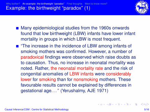
Many epidemiological studies from the 1960s onwardsfound that low birthweight (LBW) infants have lower infantmortality in groups in which LBW is most frequent.“The increase in the incidence of LBW among infants ofsmoking mothers was confirmed. However, a number ofparadoxical findings were observed which raise doubts asto causation. Thus, no increase in neonatal mortality wasnoted. Rather, the neonatal mortality rate and the risk ofcongenital anomalies of LBW infants were considerablylower for smoking than for nonsmoking mothers. Thesefavourable results cannot be explained by differences ingestational age. . . ” (Yerushalmy, AJE 1971)

Causal Inference/CSM : Centre for Statistical Methodology 5/16

Why bother? An example: the birthweight “paradox” Final thoughts Want to know more?

Example: the birthweight “paradox” (2)

those networks (15, 16), as figure 3 shows. The diagramslink variables (nodes) by arrows (directed edges) that rep-resent direct causal effects (protective or causative) of onevariable on another. DAGs are acyclic because the arrowsnever point from a given variable to any other variable in itspast (i.e., causes precede their effects); thus, one can neverstart from one variable and, following the direction of thearrows, end up at the same variable. The absence of an arrowbetween two variables indicates that the investigator be-lieves there is no direct effect (i.e., a causal effect not me-diated through other variables in the DAG) of one variableon the other (15, 17). In this article, we build upon previouspublications in which investigators used DAGs to show howstandard adjustment (stratification or regression) for vari-ables affected by exposure may create bias by introducinga spurious (noncausal) association between the exposureand the outcome (9, 10, 14).

Figure 3.1 depicts the simplest scenario, in which smok-ing affects mortality solely through a reduction of birthweight. Under this scenario, the crude mortality rate ratiofor smoking would be greater than 1, whereas the adjustedrate ratio and, equivalently, the stratum-specific rate ratiosshould be 1. Therefore, the proposed DAG in figure 3.1 isnot consistent with our findings. Note that there might becommon causes of smoking and infant mortality (e.g., socio-economic factors) that would induce confounding. For sim-plicity, we assume that our analyses are conducted withinlevels of those common causes (i.e., there is complete con-trol for confounding) and thus omit them from the graphs.

Alternatively, smokingmight affect mortality solely throughpathways not mediated by birth weight (figure 3.2). In this

case, the crude and adjusted rate ratios would be the same.Again, this is not consistent with our findings.

Figure 3.3 combines the previous two diagrams: The ef-fect of smoking is only partly mediated by birth weight. Inthis case, the adjusted rate ratio would generally differ fromthe crude rate ratio and from 1 due to the direct (i.e., notmediated by birth weight) effect of smoking on mortality,which is consistent with our findings. Actually, figure 3.3would be consistent with any finding, because figure 3.3 isa complete DAG; that is, it does not impose any restrictionson the values of the stratum-specific rate ratios. As a conse-quence, figure 3.3 is the simplest graphical representationof the theory that there is a qualitative modification of thesmoking effect by birth weight. However, most expertswould agree that figure 3.3 is an overly simplistic represen-tation of nature. In a more realistic yet still naıve causaldiagram (figure 3.4), there would be common causes ofLBW and mortality (e.g., birth defects, malnutrition). Thepresence of these risk factors (U), usually unmeasured bythe investigator, would generally induce a spurious associ-ation between smoking and mortality when the analysis wasstratified on birth weight (10, 14, 18). This (selection) biasmay explain the ‘‘paradox.’’

We now provide a heuristic explanation of why this typeof selection bias arises. To do so, we will use the simplifieddiagram shown in figure 3.5. This new diagram uses birthdefects as the unmeasured variable (U) and includes only thethree arrows that are necessary for the bias to occur: an ar-row from smoking (the exposure) to birth weight (the vari-able that the analysis is being stratified on), an arrow frombirth defects to birth weight, and an arrow from birth defects

1

10

100

1,000

1,000

2,000

3,000

4,000

1,250

2,250

3,250

4,250

1,500

2,500

3,500

4,500

1,750

2,750

3,750

4,750

Birth Weight (g)

Mor

talit

y pe

r 1,

000

Liv

ebir

ths

Nonsmokers Smokers

FIGURE 2. Birth-weight-specific infant mortality curves for infants born to smokers and nonsmokers, United States, 1991 (national linked birth/infant-death data, National Center for Health Statistics).

The Birth Weight ‘‘Paradox’’ 1117

Am J Epidemiol 2006;164:1115–1120

by guest on Septem

ber 28, 2010aje.oxfordjournals.org

Dow

nloaded from

Causal Inference/CSM : Centre for Statistical Methodology 6/16

Why bother? An example: the birthweight “paradox” Final thoughts Want to know more?

Example: the birthweight “paradox”A ‘causal inference’ view (1)

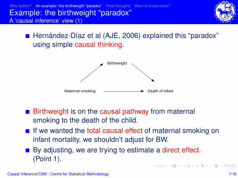
Hernandez-Dıaz et al (AJE, 2006) explained this “paradox”using simple causal thinking.

Maternal smoking

Birthweight

Death of infant

Birthweight is on the causal pathway from maternalsmoking to the death of the child.If we wanted the total causal effect of maternal smoking oninfant mortality, we shouldn’t adjust for BW.By adjusting, we are trying to estimate a direct effect.(Point 1).

Causal Inference/CSM : Centre for Statistical Methodology 7/16

Why bother? An example: the birthweight “paradox” Final thoughts Want to know more?

Example: the birthweight “paradox”A ‘causal inference’ view (2)

Maternal smoking

Birthweight

Death of infant

Congenitalbirth defect

Confounders

But there are common causes of LBW and infant mortality,eg congenital birth defects, and confounders of smokingand infant mortality. (Point 2).

Causal Inference/CSM : Centre for Statistical Methodology 8/16

Why bother? An example: the birthweight “paradox” Final thoughts Want to know more?

Example: the birthweight “paradox”A ‘causal inference’ view (3)

Maternal smoking

Birthweight

Death of infant

Congenitalbirth defect

Confounders

Stratifying on the common effect of two independentcauses induces an association between the causes.(Why?)Congenital birth defects plays the role of a confounder inthis analysis.This explains the “paradoxical” findings.

Causal Inference/CSM : Centre for Statistical Methodology 9/16

Why bother? An example: the birthweight “paradox” Final thoughts Want to know more?

Example: the birthweight “paradox”A ‘causal inference’ view (4)

Maternal smoking

Birthweight

Death of infant

Congenitalbirth defect

Confounders

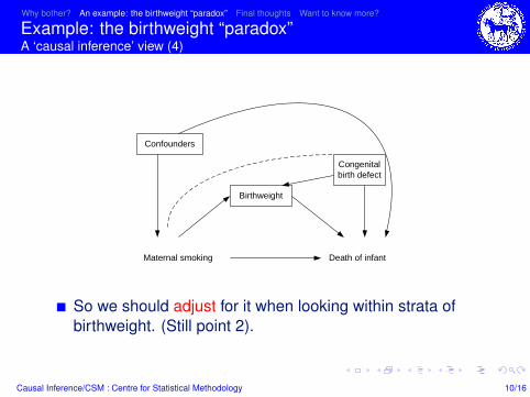
So we should adjust for it when looking within strata ofbirthweight. (Still point 2).

Causal Inference/CSM : Centre for Statistical Methodology 10/16

Why bother? An example: the birthweight “paradox” Final thoughts Want to know more?

Example: the birthweight “paradox”A ‘causal inference’ view (5)

Maternal smoking

Birthweight

Death of infant

Congenitalbirth defect

Confounders

But what if maternal smoking also causes congenital birthdefects?Now it is an intermediate confounder.Alternative methods (g-computation, ipw, g-estimation) canbe used. (Point 3).

Causal Inference/CSM : Centre for Statistical Methodology 11/16

Why bother? An example: the birthweight “paradox” Final thoughts Want to know more?

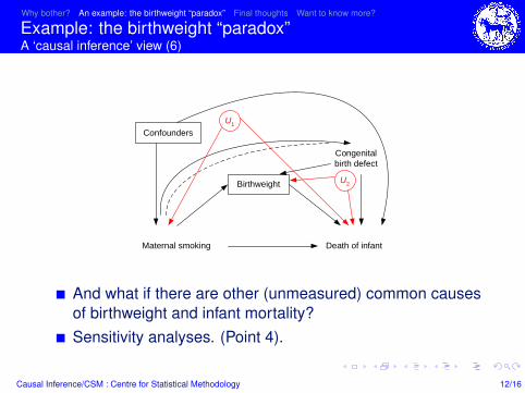
Example: the birthweight “paradox”A ‘causal inference’ view (6)

Maternal smoking

Birthweight

Death of infant

Congenitalbirth defect

ConfoundersU1

U2

And what if there are other (unmeasured) common causesof birthweight and infant mortality?Sensitivity analyses. (Point 4).

Causal Inference/CSM : Centre for Statistical Methodology 12/16

Why bother? An example: the birthweight “paradox” Final thoughts Want to know more?

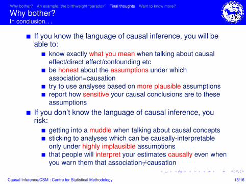
Why bother?In conclusion. . .

If you know the language of causal inference, you will beable to:

know exactly what you mean when talking about causaleffect/direct effect/confounding etcbe honest about the assumptions under whichassociation=causationtry to use analyses based on more plausible assumptionsreport how sensitive your causal conclusions are to theseassumptions

If you don’t know the language of causal inference, yourisk:

getting into a muddle when talking about causal conceptssticking to analyses which can be causally-interpretableonly under highly implausible assumptionsthat people will interpret your estimates causally even whenyou warn them that association6=causation

Causal Inference/CSM : Centre for Statistical Methodology 13/16

Why bother? An example: the birthweight “paradox” Final thoughts Want to know more?

Final thought

Always saying “. . . but association is not causation” is likeputting “this product may contain nuts” on all foodpackaging.It’s true and absolves us of all responsibility.But is it useful? Is it ethical?Causality is not an impossible word. It’s challenging,important, interesting, fun. . .

Causal Inference/CSM : Centre for Statistical Methodology 14/16

Why bother? An example: the birthweight “paradox” Final thoughts Want to know more?

If you want to know more. . .Short course

Causal Inference in Epidemiology: Recent MethodologicalDevelopmentsNovember reading week.http://www.lshtm.ac.uk/prospectus/short/causal_inference.html

Causal Inference/CSM : Centre for Statistical Methodology 15/16

Why bother? An example: the birthweight “paradox” Final thoughts Want to know more?

If you want to know more. . .Seminars/discussion groups/workshops

Join our causal inference mailing list (email me:Rhian.Daniel@LSHTM.ac.uk)Upcoming seminars:

November 1st, Manson Theatre, 1pm: “Intermediateconfounding, measurement error and missing data: a waythrough the epidemiologist’s reality?”November 19th, 12:45pm (room tbc): “The hazards ofhazard ratios” (Jonathan Bartlett)December 1st, 12:45pm (room tbc): “The regressiondiscontinuity design: redesigned for epidemiology”(Gianluca Baio, UCL & Sara Geneletti, LSE)

Causal Inference/CSM : Centre for Statistical Methodology 16/16