CERN-PH-TH/2007-048 Why CMB physics? Massimo Giovannini 1 Centro “Enrico Fermi”, Via Panisperna 89/A, 00184 Rome, Italy Department of Physics, Theory Division, CERN, 1211 Geneva 23, Switzerland Abstract The aim of these lectures is to introduce some basic problems arising in gravitation and modern cosmology. All along the discussion the guiding theme is provided by the phenomenological and theoretical properties of the Cosmic Microwave Background (CMB). These lectures have been prepared for a regular Phd course of the University of Milan-Bicocca. 1 e-mail address: [email protected]
Transcript
CERN-PH-TH/2007-048
Why CMB physics?
Massimo Giovannini 1
Centro “Enrico Fermi”, Via Panisperna 89/A, 00184 Rome, Italy
Department of Physics, Theory Division, CERN, 1211 Geneva 23, Switzerland
Abstract
The aim of these lectures is to introduce some basic problems arising in gravitation and modern
cosmology. All along the discussion the guiding theme is provided by the phenomenological and
theoretical properties of the Cosmic Microwave Background (CMB). These lectures have been
prepared for a regular Phd course of the University of Milan-Bicocca.
1 Electromagnetic emission of the observable Universe
1.1 Motivations and credits
The lectures collected in the present paper have been written on the occasion of a course prepared for
the Phd program of the University of Milan-Bicocca. Following the kind invitation of G. Marchesini
and C. Destri I have been very glad of presenting a logical collection of topics selected among the physics
of Cosmic Microwave Background (CMB in what follows). While preparing these lectures I have been
faced with the problems usually encountered in trying to introduce the conceptual foundations of
a rapidly growing field. To this difficulty one must add, as usual, that the cultural background of
Phd students is often diverse: not all Phd students are supposed to take undergraduate courses in
field theory, general relativity or cosmology. Last year, during the whole summer semester, I used to
teach a cosmology course at the technical school of Lausanne (EPFL). Using a portion of the material
prepared for that course, I therefore summarized the essentials needed for a reasonably self-contained
presentation of CMB physics. While I hope that this compromise will be appreciated, it is also clear
that a Phd course, for its own nature, imposes a necessary selection among the possible topics.
In commencing this script I wish also to express my very special an sincere gratitude to G. Cocconi
and E. Picasso. I am indebted to G. Cocconi for his advices in the preparation of the first section. I am
indebted to E. Picasso for sharing his deep knowledge of general relativity and gravitational physics
and for delightful discussions which have been extremely relevant both for the selection of topics and
for the overall spirit of the course. The encouragement and comments of L. Alvarez-Gaume have been
also greatly appreciated.
While lecturing in Milan I had many stimulating questions and comments on my presentations
from L. Girardello, G. Marchesini, P. Nason, S. Penati and C. Oleari. These interesting comments
led to an improvement of the original plan of various lectures. I also wish to express my gratitude
for the discussions with the members of the astrophysics group. In particular I acknowledge very
interesting discussions with G. Sironi on the low-frequency measurements of CMB distorsions and on
the prospects of polarization experiments. I also thank S. Bonometto and L. Colombo for stimulating
questions and advices. Last but not least, I really appreciated the lively and pertinent questions of
the Phd students attending the course. In particular, it is a pleasure to thank A. Amariti, S. Alioli,
C.-A. Ratti, E. Re and S. Spinelli.
1.2 Electromagnetic emission of the Universe
In the present section, after a general introduction to black body emission, the question reported in
the title of this paper will be partially answered. The whole observable Universe will therefore be
approached, in the first approximation, as a system emitting electromagnetic radiation. The topics to
be treated in the present section are therefore the following:
• electromagnetic emission of the Universe;
• the black-body spectrum and its physical implications;
• a bit of history of the CMB observations;
5
−9 −6 −3 0 3 6 9 12 15 18 20−14
−12
−10
−8
−6
−4
−2
6 3 0 −3 −6 −9 −12 −15 −18 −21
log(E/eV)
log
Ωγ(E
)
CMB
Radio
IR
Optical
UV x rays γ rays
Cosmic rays
log(λ/mm)
m−2 sec−1
m−2 yr−1
km−2 yr−1
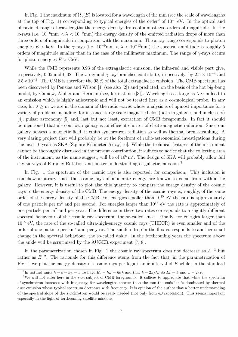
Figure 1: The (extragalactic) electromagnetic emission is illustrated. On the vertical axis the logarithm
(to base 10) of the emitted energy density is reported in units of ρcrit (see Eq. (1.6)). The logarithm
of energy of the photons is instead reported on the horizontal axis. The wavelength scale is inserted
at the top of the plot. The cosmic ray spectrum is included for comparison and in the same units used
to describe the electromagnetic contribution.
• the entropy of the CMB and its implications;
• the time evolution of the CMB temperature.
All along these lectures the natural system of units will be adopted. In this system h = c = κB = 1.
In order to pass from one system of units to the other it is useful to recall that
• hc = 197.327 MeV fm;
• K = 8.617 × 10⁻⁵ eV;
• (hc)2 = 0.389 GeV2 mbarn;
• c = 2.99792 × 1010 cm/sec.
In Fig. 1 a rather intriguing plot summarizes the electromagnetic emission of our own Universe. Only
the extra-galactic emissions are reported. On the horizontal axis we have the logarithm of the energy
of the photons (expressed in eV). On the vertical axis we reported the logarithm (to base 10) of Ωγ(E)
which is the energy density of the emitted radiation in critical units and per logarithmic interval of
photon momentum (see, for instance, Eq. (1.8)). For comparison also the associated wavelength of the
emitted radiation is illustrated (see the top of the figure) in units of mm. Figure 1 motivates the choice
of studying accurately the properties of CMB. Moreover, it can be also argued that the properties of
CMB encode, amusingly enough, not only the successes of the standard cosmological model but also
its potential drawbacks.
6
In Fig. 1 the maximum of Ωγ(E) is located for a wavelength of the mm (see the scale of wavelengths
at the top of Fig. 1) corresponding to typical energies of the order2 of 10−3 eV. In the optical and
ultraviolet range of wavelengths the energy density drops of almost two orders of magnitude. In the
x-rays (i.e. 10−6mm < λ < 10−9mm) the energy density of the emitted radiation drops of more than
three orders of magnitude in comparison with the maximum. The x-ray range corresponds to photon
energies E > keV. In the γ-rays (i.e. 10−9mm < λ < 10−12mm) the spectral amplitude is roughly 5
orders of magnitude smaller than in the case of the millimeter maximum. The range of γ-rays occurs
for photon energies E > GeV.
While the CMB represents 0.93 of the extragalactic emission, the infra-red and visible part give,
respectively, 0.05 and 0.02. The x-ray and γ-ray branches contribute, respectively, by 2.5 × 10⁻⁴ and
2.5×10⁻⁵. The CMB is therefore the 93 % of the total extragalactic emission. The CMB spectrum has
been discovered by Penzias and Wilson [1] (see also [2]) and predicted, on the basis of the hot big-bang
model, by Gamow, Alpher and Herman (see, for instance,[3]). Wavelengths as large as λ ∼ m lead to
an emission which is highly anisotropic and will not be treated here as a cosmological probe. In any
case, for λ ≥ m we are in the domain of the radio-waves whose analysis is of upmost importance for a
variety of problems including, for instance, large scale magnetic fields (both in galaxies and in clusters)
[4], pulsar astronomy [5] and, last but not least, extraction of CMB foregrounds. In fact it should
be mentioned that also our own galaxy is an efficient emitter of electromagnetic radiation. Since our
galaxy possess a magnetic field, it emits synchrotron radiation as well as thermal bremsstrahlung. A
very daring project that will probably be at the forefront of radio-astronomical investigations during
the next 10 years is SKA (Square Kilometer Array) [6]. While the technical features of the instrument
cannot be thoroughly discussed in the present contribution, it suffices to notice that the collecting area
of the instrument, as the name suggest, will be of 106 m2. The design of SKA will probably allow full
sky surveys of Faraday Rotation and better understanding of galactic emission 3
In Fig. 1 the spectrum of the cosmic rays is also reported, for comparison. This inclusion is
somehow arbitrary since the cosmic rays of moderate energy are known to come from within the
galaxy. However, it is useful to plot also this quantity to compare the energy density of the cosmic
rays to the energy density of the CMB. The energy density of the cosmic rays is, roughly, of the same
order of the energy density of the CMB. For energies smaller than 1015 eV the rate is approximately
of one particle per m2 and per second. For energies larger than 1015 eV the rate is approximately of
one particle per m2 and per year. The difference in these two rates corresponds to a slightly different
spectral behaviour of the cosmic ray spectrum, the so-called knee. Finally, for energies larger than
1018 eV, the rate of the so-called ultra-high-energy cosmic rays (UHECR) is even smaller and of the
order of one particle per km2 and per year. The sudden drop in the flux corresponds to another small
change in the spectral behaviour, the so-called ankle. In the forthcoming years the spectrum above
the ankle will be scrutinized by the AUGER experiment [7, 8].
In the parametrization chosen in Fig. 1 the cosmic ray spectrum does not decrease as E−3 but
rather as E−2. The rationale for this difference stems from the fact that, in the parametrization of
Fig. 1 we plot the energy density of cosmic rays per logarithmic interval of E while, in the standard
2In natural units h = c = kB = 1 we have Ek = hω = hc k and that k = 2π/λ. So Ek = k and ω = 2πν.3We will not enter here in the vast subject of CMB foregrounds. It suffices to appreciate that while the spectrum
of synchrotron increases with frequency, for wavelengths shorter than the mm the emission is dominated by thermal
dust emission whose typical spectrum decreases with frequency. It is opinion of the author that a better understanding
of the spectral slope of the synchrotron would be really needed (not only from extrapolation). This seems important
especially in the light of forthcoming satellite missions.
7
parametrization the plot is in terms of dρcrays/dE. It is important to stress that while the CMB
represents the 93 % of the extragalactic emission, the diffuse x-ray and γ-ray backgrounds are also of
upmost importance for cosmology. Various experiments have been dedicated to the study of the x-ray
background such as ARIEL, EINSTEIN, GINGA, ROSAT and, last but not least, BEPPO-SAX, an
x-ray satellite named after Giuseppe (Beppo) Occhialini. Among γ-ray satellites we shall just mention
COMPTON, EGRET and the forthcoming GLAST.
1.3 The black-body spectrum ad its physical implications
According to Fig. 1, in the mm range the electromagnetic spectrum of the Universe is very well fitted
by a black-body spectrum: if we would plot the error bars magnified 400 times they would still be
hardly distinguishable from the thickness of the curve. Starting from the discovery of Penzias and
Wilson [1] various groups confirmed, independently, the black-body nature of this emission (see below,
in this section, for an oversimplified account of the intriguing history of CMB observations). As it is
well known the black-body has the property of depending only upon one single parameter which is the
temperature Tγ of the photon gas at the thermodynamic equilibrium. Such a temperature is given by
Tγ = 2.725 ± 0.001 K. (1.1)
According to Wien’s law λTγ = 2.897 × 10⁻³ m K. Thus, as already remarked the wavelength of the
maximum will be λ ≃ mm. For a photon gas in thermodynamic equilibrium the energy density of the
emitted radiation is given by
dργ = g × ω × d3ω
(2π)3× nω, (1.2)
where g is the number of intrinsic degrees of freedom (g = 2 in the case of photons) and nω is the
Bose-Einstein occupation number:
nω =1
eω/Tγ − 1. (1.3)
Since in natural units, Ek = k = ω, the energy density of the emitted radiation per logarithmic interval
of frequency is given by:dργd ln k
=1
π2
k4
ek/Tγ − 1. (1.4)
Equation (1.4) allows also to compute the total (i.e. integrated) energy density ργ . The differential
spectrum (1.4) can then be referred to the integrated energy density expressed, in turn, in units of the
critical energy density. From Eq. (1.4) the integrated energy density of photons is simply given by
ργ(t0) =T 4γ
π2
∫ ∞
0
x3
ex − 1=π2
15T 4γ , (1.5)
where the ratio x = k/Tγ has been defined and where the integral in the second equality is given by
π4/15.
A useful way of measuring energy densities is to refer them to the critical energy density of the
Universe (see section 2 for a more detailed discussion of this important quantity). According to the
present data it seems that the critical energy density indeed coincides with the total energy density
of the Universe. This is just because experimental data seem to favour a spatially flat Universe. The
critical energy density today is given by:
ρcrit =3H2
0
8πG= 1.88 × 10⁻²⁹ h2
0 g cm−3 = 1.05 × 10⁻⁵ h20 GeV cm−3, (1.6)
8
where h0 (often assumed to be ∼ 0.7 for the purpose of numerical estimates along these lectures) mea-
sures the indetermination on the present value of the Hubble parameter H0 = 100 km sec−1 Mpc−1h0.
From the second equality appearing in Eq. (1.6), recalling that the proton mass is mp = 0.938 GeV,
it is also possible to deduce
ρcrit = 5.48(
h0
0.7
)2 mp
m3, (1.7)
showing that, the critical density is, grossly speaking, the equivalent of 6 proton masses per cubic
meter.
From Eqs. (1.4) and (1.6) we can obtain the energy density of photons per logarithmic interval of
energy and in critical units, i.e.
Ωγ(k) =1
ρcrit
dργd ln k
. (1.8)
Recalling that Ek = k (and neglecting the subscript) we have that
Ωγ(E) =15
π4Ωγ0
x4
ex − 1, (1.9)
where
x =E
Tγ= 4.26 × 10³
(
E
eV
)
,
Ωγ0 =ργ(t0)
ρcrit= 2.471 × 10⁻⁵ h−2
0 . (1.10)
The quantities Ωγ(E) and Ωγ0 are physically different: Ωγ0 is the ratio between the total (present)
energy density of CMB photons and the critical energy density and it is independent on the frequency.
It can be explicitly verified that, inserting the numerical value of Tγ and ρc (i.e. Eqs. (1.1) and (1.6)),
the figure of Eq. (1.10) is swiftly reproduced.
The spectrum of Eq. (1.9) can be also plotted in terms of the frequency. Recalling that, in natural
units, ν = 2πk and that
x =k
Tγ= 0.01765
(
ν
GHz
)
, (1.11)
the spectrum Ωγ(ν) is reported in Fig. 2. It should be borne in mind that the CMB spectrum could
be distorted by several energy-releasing processes. These distorsions have not been observed so far.
In particular we could wander if a sizable chemical potential is allowed. The presence of a chemical
potential will affect the Bose-Einstein occupation number which will become, in our rescaled notations
nBk = (ex+µ0 − 1)−1. Now the experimental data imply that |µ0| < 9 × 10⁻⁵ (95% C.L.).
It is useful to mention, at this point, the energy density of the CMB in different units and to
compare it directly with the cosmic ray spectrum as well as with the energy density of the galactic
magnetic field. In particular we will have that
ργ =π2
15T 4γ = 2 × 10−51
(
Tγ2.725
)4
GeV4, (1.12)
ρB =B2
8π= 1.36 × 10−52
(
B
3µG
)2
GeV4. (1.13)
From Eqs. (1.12) and (1.13) it follows that the CMB energy density is roughly comparable with the
magnetic energy density of the galaxy. Furthermore ρcrays ≃ ρB.
9
−1 −0.5 0 0.5 1 1.5 2 2.5 3 3.5−16
−14
−12
−10
−8
−6
−4
log (ν/GHz)
log
h 02 Ωγ(ν
)
Figure 2: The CMB logarithmic energy spectrum here illustrated in terms of the frequency.
1.4 A bit of history of CMB observations
The black-body nature of CMB emission is one of the cornerstones of the Standard cosmological model
whose essential features will be introduced in section 2. The first measurement of the CMB spectrum
goes back to the work of Penzias and Wilson [1]. The Penzias and Wilson measurement referred
to a wavelength of 7.35 cm (corresponding to 4.08 GHz). They estimated a temperature of 3.5 0K.
Since the Penzias and Wilson measurement the black-body nature of the CMB spectrum has been
investigated and confirmed for a wide range of frequencies extending from 0.6 GHz [10] (see also [11])
up to 300 GHz. The history of the measurements of the CMB temperature is a subject by itself which
has been reviewed in the excellent book of B. Patridge [12]. Before 1990 the measurements of CMB
properties have been conducted always through terrestrial antennas or even by means of balloon borne
experiments. In the nineties the COBE satellite [13, 14, 15, 16, 17, 18, 19, 20] allowed to measure the
properties of the CMB spectrum in a wide range of frequencies including the maximum (see Fig. 2).
The COBE satellite had two instruments: FIRAS and DMR.
The DMR was able to probe the angular power spectrum4 up to ℓ ≃ 26. As the name says, DMR
was a differential instrument measuring temperature differences in the microwave sky. The angular
resolution of a given instrument, i.e. ϑ, is related to the maximal multipole probed in the sky according
to the approximate relation ϑ ≃ π/ℓ. Consequently, since the angular resolution of COBE was 70,
the maximal ℓ accessible to that experiment was ℓ ≃ 1800/70 ∼ 26. Since the angular resolution of
WMAP is 0.230, the corresponding maximal harmonic probed by WMAP will be ℓ ≃ 1800/0.230 ∼ 783.
Finally, the Planck experiment, to be soon launched will achieve an angular resolution of 5′, implying
ℓ ≃ 1800/5′ ∼ 2160.
After the COBE mission, various experiments attempted the exploration of smaller angular sep-
aration, i. e. larger multipoles. A definite convincing evidence of the existence and location of the
first peak in the Cℓ spectrum came from the Boomerang [21, 22] , Dasi [23] and Maxima [24] ex-
4While the precise definition of angular power spectrum will be given later on, here it suffices to recall that
ℓ(ℓ + 1)Cℓ/(2π) measures the degree of inhomogeneity in the temperature distribution per logarithmic interval of ℓ.
Consequently, a given multipole ℓ can be related to a given spatial structure in the microwave sky: small ℓ will corre-
spond to low wavenumbers, high ℓ will correspond to larger wave-numbers.
10
Figure 3: Some CMB anisotropy data are reported (figure adapted from [27]): WMAP data (filled
circles); VSA data (shaded circles) [28]; CBI data (squares) [35, 36]; ACBAR data (triangles) [37].
periments. Both Boomerang and Maxima were balloon borne (bolometric) experiments. Dasi was a
ground based interferometer. The data points of these last three experiments explored multipoles up
to 1000, determining the first acoustic oscillation (in the jargon the first Doppler peak) for ℓ ≃ 220.
Another important balloon borne experiments was Archeops [25] providing interesting data for the
region characterizing the first rise of the Cℓ spectrum. Some other useful references on earlier CMB
experiments can be found in [26].
The Cℓ spectrum, as measured by different recent experiments is reported in Fig. 3 (adapted
from Ref. [27]). At the moment the most accurate determinations of CMB observables are derived
from the data of WMAP (Wilkinson Microwave Anisotropy Probe). The first release of WMAP data
are the subject of Refs. [29, 30, 31, 32]. The three-years release of WMAP data is discussed in
Refs. [33, 34]. The WMAP data (filled circles in Fig. 3) provided, among other important pieces
of information the precise determination of the position of the first peak (i.e. ℓ = 220.1 ± 0.8 [30])
the evidence of the second peak. The WMAP experiment also measured temperature-polarization
correlations providing a distinctive signature (the so-called anticorrelation peak in the temperature-
polarization power spectrum for ℓ ∼ 150) of primordial adiabatic fluctuations (see sections 8 and 9
and, in particular Fig. 27). To have a more detailed picture of the evolution and relevance of CMB
experiments we refer the reader to Ref. [43] (for review of the pre-1994 status of the art) and Ref.
[44] for a review of the pre-2002 situation). The rather broad set of lectures by Bond [45] may also be
usefully consulted.
In recent years, thanks to combined observations of CMB anisotropies [29, 30], Large scale structure
[38, 39], supernovae of type Ia [40], big-bang nucleosyntheis [41], some kind of paradigm for the
evolution of the late time (or even present) Universe emerged. It is normally called by practitioners
ΛCDM model or even, sometimes, “concordance model”. The terminology of ΛCDM refers to the fact
that, in this model, the dominant (present) component of the energy density of the Universe is given
by a cosmological constant Λ and a fluid of cold dark matter particles interacting only gravitationally
with the other (known) particle species such as baryons, leptons, photons. According to this paradigm,
our understanding of the Universe can be summarized in two sets of cosmological parameters: the
first set of parameters refers to the homogeneous background, the second set of parameters to the
inhomogeneities. So, on top of the indetermination on the (present) Hubble expansion rate, i.e. h0,
there are various other parameters such as:
11
• the (present) dark energy density in critical units5, i.e. h20ΩΛ0;
• the (present) cold dark matter (CDM in what follows) energy density, i.e. h20Ωc0;
• the (present) baryon energy density, i.e. h20Ωb0;
• the (present) photon energy density (already introduced) h20Ωγ0;
• the (present) neutrino energy density, i.e. h20Ων0;
• the optical depth at reionization (denoted by ǫ but commonly named τ which denotes instead,
in the present lectures, the conformal time coordinate, see section 2);
• the spectral index of the primordial (adiabatic) mode for the scalar fluctuations nr;
• the amplitude of the curvature perturbations Aad;
• the bias parameter (related to large scale structure).
To this more or less standard set of parameters one can also add other parameters reflecting a finer
description of pre-decoupling physics:
• the neutrinos are, strictly speaking, massive and their masses can then constitute an additional
set of parameters;
• the dark energy may not be exactly a cosmological constant and, therefore, the barotropic index
of dark energy may be introduced as the ratio between the pressure of dark energy and its energy
density (similar argument can entail also the introduction of the sound speed off dark energy);
• the spectral index may not be constant as a function of the wave-number and this consideration
implies a further parameter;
• in the commonly considered inflationary scenarios there are not only scalar (adiabatic) modes
but also tensor modes and this evidence suggests the addition of the relative amplitude and
spectral index of tensor perturbations, i.e., respectively, r and nT.
Different parameters can be introduced in order to account for even more daring departures from the
standard cosmological lore. These parameters include
• the amplitude and spectral index of primordial non-adiabatic perturbations;
• the amplitude and spectral index of the correlation between adiabatic and non-adiabatic modes;
• a primordial magnetic field which is fully inhomogeneous and characterized, again, by a given
spectrum and an amplitude.
5Instead of giving the critical fraction of the total energy density alone, it is common practice to multiply this figure
by h20 so that the final number will be independent of h0.
12
This list can be easily completed by other possible (and physically reasonable) parameters. We just
want to remark that the non-adiabatic modes represent a whole set of physical parameters since,
as it will be swiftly discussed, there are 4 non-adiabatic modes. Consequently, already a thorough
parametrization of the non-adiabatic sector will entail, in its most general incarnation, 4 spectral
indices, 4 spectral amplitudes and the mutual correlations of each non-adiabatic mode with the adia-
batic one. Having said this it is important to stress that the lectures will not deal with the problem
of data analysis (or parameter extraction from the CMB data). The purpose of the present lectures,
as underlined before in this introduction, will be to use CMB as a guiding theme for the formulation
of a consistent cosmological framework which might be in sight but which is certainly not yet present.
1.5 The entropy of the CMB and its implications
The pressure of black-body photons is simply pγ = ργ/3. Since the chemical potential exactly vanishes
in the case of a photon gas at the thermodynamic equilibrium, the entropy density of the black-body
is given, through the fundamental identity of thermodynamics (see Appendix B), by
sγ =SγV
=ργ + pγTγ
=4
45π2T 3
γ , (1.14)
where Sγ is the entropy and V is a fiducial volume. Equation (1.14) implies that the entropic content
of the present Universe is dominated by the species that are relativistic today (i.e. photons) and that
the total entropy contained in the Hubble volume, i.e. Sγ is huge. The Hubble volume can be thought
as the present size of our observable Universe and it is roughly given by VH = 4πH−30 /3. Thus, we
will have that
Sγ =4
3πsγH
−30 ≃ 1.43 × 1088
(
h0
0.7
)−3
. (1.15)
The figure provided by Eq. (1.15) is still one of the major problems of the standard cosmological
model. Why is the entropy of the observable Universe so large? Note for the estimate of Eq. (1.15) it
is practical to express both Tγ and H0 in Planck units, namely:
Tγ = 1.923 × 10⁻³² MP, H0 = 1.22 × 10−61(
h0
0.7
)
MP. (1.16)
It is clear that the huge value of the present entropy is a direct consequence of the smallness of H0 in
Planck units. This implies that Tγ/H0 ≃ 1.57 × 1029. Let us just remark that the present estimate
only concerns the usual entropy, i.e. the thermodynamic entropy. Considerations related with the
validity (also in the early Universe) of the second law of thermodynamics seem to suggest that also
the entropy of the gravitational field itself may play a decisive role. While some motivations seem
to be compelling there is no consensus, at the moment, on what should be the precise mathematical
definition of the entropy of the gravitational field. This remark is necessary since we should keep our
minds open. It may well be that the true entropy of the Universe (i.e. the entropy of the sources and
of the gravitational field) is larger than the one computed in Eq. (1.15). Along this direction it is
possible to think that the maximal entropy that can be stored inside the Hubble radius rH is of the
order of a black-hole with radius rH which would give
r2HM
2P ≃ 10122. (1.17)
13
In connection with Eq. (1.16), it is also useful to point out that the critical density can be expressed
directly in terms of the fourth power of the Planck mass, i.e. :
ρcrit =3
8πH2
0M2P = 1.785 × 10−123
(
h0
0.7
)2
M4P. (1.18)
The huge hierarchy between the critical energy density of the present Universe and the Planckian
energy density is, again, a direct reflection of the hierarchy between the Hubble parameter and the
Planck mass. Such a hierarchy would not be, by itself, problematic. The rationale for such a statement
is connected to the fact that in the SCM the energy densities as well as the related pressures decrease
as the Universe expand. However, it turns out that, today, the largest portion of the energy density
of the Universe is determined by a component called dark energy. The term dark is a coded word of
astronomy. It means that a given form of matter neither absorbs nor emit radiation. Furthermore the
dark energy is homogeneously distributed and, unlike dark matter, is not concentrated in the galactic
halos and in the clusters of galaxies. Now, one of the chief properties of dark energy is that it is not
affected by the Universe expansion and this is the reason why it is usually parametrized in terms of a
cosmological constant. measurements tell us that ρΛ ≃ 0.7ρcrit which implies, from Eq. (1.18) that
ρΛ ≃ 1.24 × 10−123 M4P. (1.19)
Since ρΛ does not decreases with the expansion of the Universe, we have also to admit that Eq. (1.19)
was enforced at any moment in the life of the Universe and, in particular at the moment when the
initial conditions of the SCM were set. A related way of phrasing this impasse relies on the field
theoretical interpretation of the cosmological constant. In field theory we do know that the zero-point
(vacuum) fluctuations have an energy density (per logarithmic interval of frequency) that goes as k4.
Now, adopting the Planck mass as the ultraviolet cut-off we would be led to conclude that the total
energy density of the zero-point vacuum fluctuations would be of the order of M4P. On the contrary,
the result of the measurements simply gives us a figure which is 122 orders of magnitude smaller.
The expression of the black-body spectrum also allows the calculation of the photon concentration.
Recalling that, in the case of photons, dn = (k3nk/π2)d log k we have, after integration over k that the
concentration of photons is given by
n =2ζ(3)
π2T 3γ ≃ 411 cm−3 (1.20)
where ζ(r) is the Riemann zeta function with argument r.
1.6 The time evolution of the CMB temperature
In summary we can therefore answer, in the first approximation, to the title of this lecture series:
• in the electromagnetic spectrum the contribution of the CMB is by far larger than the other
branches and constitutes, roughly, the 93 % of the whole emission;
• the CMB energy density is comparable with (but larger than) the energy density of cosmic rays;
• the CMB energy density is a tiny fraction of the total energy density of the Universe (more
precisely 24 millionth of the critical energy density);
14
• the CMB dominates the total entropy of the present Hubble patch: Sγ ≃ 1088.
The fact that we observe a CMB seems implies that CMB photons are in thermal equilibrium at
the temperature Tγ . This occurrence strongly suggests that the evolution of the whole Universe must
be somehow adiabatic. This observation is one of the cornerstones of the standard cosmological model
(SCM) whose precise formulation will be given in the following section.
In a preliminary perspective, the following naive observation is rather important. Suppose that
the spatial coordinates expand thanks to a time-dependent rescaling. Consequently the wave-numbers
will be also rescaled accordingly, i.e.
~x0 → ~x = a(t)~x0, ~k0 → ~k =~k0
a(t). (1.21)
In the jargon ~k0 is commonly referred to as the comoving wave-number (which is insensitive to the
expansion), while ~k is the physical wave-number. Consider then the number of photons contained in
an infinitesimal element of the phase-space and suppose that the whole Universe expands according
to Eq. (1.21). At a generic time t1 we will then have
dnk(t1) = nk(t1)d3k1d
3x1. (1.22)
At a generic time t2 > t1 we will have, similarly,
dnk(t2) = nk(t2)d3k2d
3x2. (1.23)
By looking at Eqs. (1.22) and (1.23) it is rather easy to argue that dnk(t1) = dnk(t2) provided
nk(t1) = nk(t2). By looking at the specific form of the Bose-Einstein occupation number it is clear
that the latter occurrence is verified provided k(t1)/Tγ(t1) = k(t2)/Tγ(t2). From this simple argument
we can already argue an important fact: the black-body distribution is preserved under the rescaling
(1.21) provided the black-body temperature scales as the inverse of the scale factor a(t), i.e.
Tγ0 → Tγ =Tγ0a(t)
. (1.24)
The property summarized in Eq. (1.24) holds also in the context of the SCM where a(t) will be correctly
defined as the time-dependent scale factor of a Friedmann-Robertson-Walker (FRW) Universe. The
physical consequence of Eq. (1.24) is that the temperature of CMB photons is higher at higher redshifts
(see Appendix A for a definition of redshift). More precisely:
Tγ = (1 + z)Tγ0. (1.25)
This consequence of the theory can be tested experimentally [46]. In short, the argument goes as
follows. The CMB will populate excited levels of atomic and molecular species when the energy
separations involved are not too different from the peak of the CMB emission. The first measurement
of the local CMB temperature was actually made with this method by using the fine structure lines of
CN (cyanogen) [47]. Using the same philosophy it is reasonable to expect that clouds of other chemical
elements (like Carbon, in Ref. [46]) may be sensitive to CMB photons also at higher redshifts. For
instance in [46] measurements were performed at z = 1.776 and the estimated temperature was found
to be of the order of Tγ(z) ≃ 7.5 0K. These measurements are potentially very instructive but have
15
been a bit neglected, in the recent past, since the attention of the community focused more on the
properties of CMB anisotropies.
For the limitations imposed to the present script it is not possible to treat in detail the very
interesting physics of another important effect that gives us important informations concerning the
CMB and its primeval origin. This effect should be anyway mentioned and it is called Sunyaev-
Zeldovich effect [48, 49, 50]. The physics of this effect is, in a sense, rather simple. If you have a
cluster of galaxies, that cluster o galaxies has a deep potential well and on the average, by the virial
theorem, its kinetic motion is of the order of few keV. So some fraction of the hot gas can get ionized
and we will have ionized plasma around. That plasma emits x-rays that, for instance, the ROSAT
satellite has seen 6. Now the CMB will sweep the whole space. By looking at a direction where there is
nothing between the observer and the last scattering surface the radiation arrives basically unchanged
except for the effect due to the expansion of the Universe. But if the observation is now made along
a direction passing through a cluster of galaxies, some small fraction of the CMB photons (roughly
one over 1000 CMB photons) will be scattered by the hot gas. Because the gas is actually hot, there
is more probability that photons will be scattered at high energy rather than at low energy. They
will also be scattered almost at isotropic angle. The bottom line is that the CMB spectrum along a
line of sight that crosses a cluster of galaxies will have a slight excess of high energy photons and a
slight deficiency of low energy photons. So if you see this effect (as we do) it means that the CMB
photons come from behind the clusters. Some of these clusters are at redshift 0.07 < z < 1.03. The
measurements of the Sunyaev-Zeldovich effect have been attempted for roughly two decades but in
the last decade a remarkable progress has been made. As already mentioned, the Sunyaev-Zeldovich
effect tells that the CMB is really an extra-galactic radiation.
6It is actually interesting, incidentally, that from the ROSAT full sky survey (allowing to determine the surface
brightness of various clusters in the x-rays), the average electron density has been determined can be determined [51]
and this allowed interesting measurements of magnetic fields inside a sample of Abell clusters.
16
2 From CMB to the standard cosmological model
Various excellent publications treat the essential elements of the Standard Cosmological Model (SCM
in what follows) within different perspectives (see, for instance, [52, 53, 54, 55]). The purpose here will
not be to present the conceptual foundations SCM but to introduce its main assumptions and its most
relevant consequences with particular attention to those aspects and technicalities that are germane
to our theme, i.e. CMB physics.
It should be also mentioned that there are a number of relatively ancient papers that can be usefully
consulted to dig out both the historical and conceptual foundations of the SCM. In the he issue number
81 of the “Uspekhi Fizicheskikh Nauk” , on the occasion of the seventy-fifth anniversary of the birth of
A. A. Friedmann, a number of rather interesting papers were published. Among them there is a review
article of the development of Friedmannian cosmology by Ya. B. Zeldovich [56] and the inspiring paper
of Lifshitz and Khalatnikov [57] on the relativistic treatment of cosmological perturbations.
Reference [56] describes mainly Friedmann’s contributions [58]. Due attention should also be
paid to the work of G. Lemaıtre [59, 60, 61] that was also partially motivated by the debate with A.
Eddington [62]. According to the idea of Eddington the world evolved from an Einstein static Universe
and so developed “infinitely slowly from a primitive uniform distribution in unstable equilibrium” [62].
The point of view of Lemaıtre was, in a sense, more radical since he suggested, in 1931, that the
expansion really did start with the beginning of the entire Universe. Unlike the Universe of some
modern big-bang cosmologies, the description of Lemaıtre did not evolve from a true singularity but
from a material pre-Universe, what Lemaıtre liked to call “primeval atom” [61]. The primeval atom
was a unique atom whose atomic weight was the total mass of the Universe. This highly unstable atom
would have experienced some type of fission and would have divided into smaller and smaller atoms by
some kind of super-radioactive processes. The perspective of Lemaıtre was that the early expansion
of the Universe could be a well defined object of study for natural sciences even in the absence of a
proper understanding of the initial singularity. The discussion of the present section follows four main
lines:
• firstly the SCM will be formulated in his essential elements;
• then the matter content of the present Universe will be introduced as it emerges in the concor-
dance model;
• the (probably cold) future of our own Universe will be swiftly discussed;
• finally the (hot) past of the Universe will be scrutinized in connection with the properties of the
CMB.
Complementary discussions on the concept of distance in cosmology and on the kinetic description of
hot plasmas are collected, respectively, in Appendix A and in Appendix B.
2.1 The standard cosmological model (SCM)
The standard cosmological model (SCM) rests on the following three important assumptions:
• for typical length-scales larger than 50 Mpc the Universe is homogeneous and isotropic;
17
• the matter content of the Universe can be parametrized in terms of perfect barotropic fluids;
• the dynamical law connecting the evolution of the sources to the evolution of the geometry is
provided by General Relativity (GR).
2.1.1 Homogeneity and isotropy
The assumption of homogeneity and isotropy implies that the geometry of the Universe is invariant
for spatial roto-translations. In four space-time dimensions the metric tensor will have 10 independent
components. Using homogeneity and isotropy the ten independent components can be reduced from
10 to 4 (having taken into account the 3 spatial rotation and the 3 spatial translations). The most
general form of a line element which is invariant under spatial rotations and spatial translations can
Finally, in the present Universe, as discussed in section 1 there is also radiation. In particular we
will have that
h20ΩR0 = h2
0Ωγ0 + h20Ων0 + h2
0Ωgw0, (2.52)
where Ων0 denotes the contribution of neutrinos and Ωg0 the contribution of relic gravitons. In Eq.
(2.52) we will have
h20Ωγ0 = 2.47 10−5, h2
0Ων0 = 1.68 10−5, h20Ωgw0 < 10−11. (2.53)
The contribution of relic gravitons is, today, smaller than 10−11 this bound stems from the analysis of
the integrated Sachs-Wolfe contribution which will be discussed later in this set of lectures (see section
7). If neutrinos have masses smaller than the meV they are today non-relativistic and, in principle,
should not be counted as radiation. However, since the temperature of CMB was, in the past, much
larger (as it will be discussed below), they will be effectively relativistic at the moment when matter
decouples from radiation. Since, along these lectures, we will be primarily interested in the physics
of CMB we will assume that neutrinos are effectively massless. To be more precise, we can say that
current oscillation data require at least one neutrino eigenstate to have a mass exceeding 0.05 eV. In
this minimal case h20Ων0 ≃ 5 × 10⁻⁴ so that the neutrino contribution to the matter budget will be
negligibly small. However, a nearly degenerate pattern of mass eigenstates could allow larger densities,
since oscillation experiments only measure differences in the values of the squared masses.
2.3 The future of the Universe
From the analysis of the luminosity distance (versus the redshift) it appears that type-Ia supernovae
are dimmer than expected and this suggests that at high redshifts (i.e. z ≥ 1) the Universe is effectively
accelerating [40]. The redshift z is defined (see Appendix A for further details) as
1 + z =a0
a, (2.54)
where a0 is the present value of the scale factor and a denotes a generic stage of expansion preceding the
present epoch (i.e. a < a0). The concept of redshift (see Appendix A) is related with the observation
that, in an expanding Universe, the spectral lines of emitted radiation become more red (i.e. they
redshift, they become longer) than in the case when the Universe does not expand. Given the matter
content of the present Universe, its destiny can be guessed by using the FL equations and by integrating
26
them forward in time. From Eq. (2.32), with simple algebra, it is possible to obtain the following
equation:
dα
dx=
√
ΩM0
α+ ΩΛ0α2 + Ωk +
ΩR0
α2, (2.55)
where the following rescaled variables have been defined:
α =a
a0, x = H0t, Ωk = − k
a20H
20
, (2.56)
and the quantity with subscripts 0 always refer to the present time 11. To derive Eq. (2.55) it must also
be borne in mind that a first integration of the covariant conservation equations leads to the following
relations:
ρR = ρR0
(
a0
a
)4
, ρM = ρM0
(
a0
a
)3
, ρΛ = ρΛ0. (2.57)
From Eq. (2.55), different possibilities exist for the future dynamics of the Universe. These possibilities
depend on the relative weight of the various physical components of the present Universe. In the case
ΩΛ0 Eq. (2.55) reduces to∫
√αdα√
ΩM0 + Ωkα= H0(t− t0). (2.58)
If Ωk = 0, a(t) expands forever with a(t) ∼ t2/3 (decelerated expansion). If Ωk < 0 (closed Universe)
the Universe will collapse in the future an for a critical value αcoll ≃ ΩM0/|Ωk|. Finally, if Ωk > 0 (open
Universe) the geometry will expand forever in a decelerated way. Notice that, in Eq. (2.58) the role of
radiation has been neglected since radiation is subleading today and it will be even more subleading
in the future since it decreases faster than matter and faster than the dark energy.
If ΩΛ0 6= 0 and Ωk = 0 Eq. (2.55) can be solved in explicit terms with the result that
a
a0=(
ΩM0
ΩΛ0
)1/3
sinh[
3
2
√
ΩΛ0H0(t− t0)]2/3
. (2.59)
This solution interpolates between a matter-dominated Universe expanding in a decelerated way as
t2/3 and an exponentially expanding Universe which is also accelerating. To get to Eq. (2.59), Eq.
(2.55) can be written as∫
√αdα
√
1 + ΩΛ0
ΩM0α3
=√
ΩM0 dx. (2.60)
By introducing the auxiliary variable
α3/2
√
ΩΛ0
ΩM0
= y, (2.61)
we do obtain∫
dy√1 + y2
=3
2
√
ΩΛ0 H0 (t− t0). (2.62)
Finally, by introducing a second auxiliary variable y = sinh β the integral can be readily solved and
Eq. (2.59) reproduced. While the discussion for Ωk 6= 0, ΩΛ0 6= 0 and ΩM0 6= 0 is more complicated
and will not be treated here, it is also clear that given the matter content of the present Universe, it
11Notice that k and Ωk have opposite sign. While it is useful to define Ωk as a critical fraction, it may also engender
unwanted confusions which are related to the fact that, physically, the spatial curvature is not a further form of matter.
With these caveats the use of Ωk is rather practical.
27
is reasonable to expect that the, in the future, the Universe will accelerate faster and faster while the
role of non relativistic matter (and of radiation) will be progressively negligible.
There are a number of ways in which the kinematical features of the present Universe can be
observationally accessible. The main tool is represented by the various distance concepts used by
astronomers. The three useful distance measures that could be mentioned are (see Appendix A for
further details on the derivation of the explicit expressions):
• the distance measure (denoted with re(z) in Appendix A and often denoted with DM(z) in the
literature);
• the angular diameter distance DA(z);
• the luminosity distance.
These three distances are all functions of the redshift z and of the (present) critical fractions of
matter, dark energy, radiation and curvature, i.e., respectively, ΩM0, ΩΛ0, ΩR0, and Ωk. In practice,
the dependence upon ΩR0 can be dropped and it becomes relevant for very large redshift, i.e. z ≃ 10.
The three distances introduced in the aforementioned list of items are integrated quantities in
the sense that they depend upon the integral of the inverse of the Hubble parameter from 0 to the
generic redshift z (see Appendix A for a derivation). The angular diameter distance and the luminosity
distance are related to re(z) as
DA(z) =a0re(z)
1 + z, DL(z) = a0re(z)(1 + z), (2.63)
where a0 is the present value of the scale factor that could be conventionally normalized to 1. The
distance measure has been denoted by re since it represents the coordinate distance (defined in the
FRW line element) once the origin of the coordinate system is placed in the Milky way. The angular
diameter distance gives us the possibility of determining the distance of an object by measuring its
angular size in the sky. Of course to conduct successfully a measurement we must have a set of standard
rulers, i.e. a set of objects that have, at different redshifts, the same size.
The luminosity distance gives us the possibility of determining the distance of an object from its
apparent luminosity. Of course, as in the case of the angular diameter distance, to complete successfully
the measurement we would need a set of standard candles , i.e. a set of object with the same absolute
luminosity.
In Figs. 4, 5 and 6 the three concepts of distance introduced above are illustrated. In Fig. 4 the
distance measure is illustrated in the case of three models. The lowest (dashed) curve holds in the
case of a flat Universe with ΩM0 = 1. The intermediate (dot-dashed) curve holds in the case of a flat
Universe with ΩM0 = 1/3 and ΩΛ0 = 2/3. Finally the upper curve (full line) holds in the case of an
open Universe dominated by the spatial curvature (i.e. ΩM0 = ΩΛ0 = 0 and Ωk = 1). The angular
diameter distance is reported in Fig. 5 for the same sample of models described by Fig. 4. For large
redshift, the angular diameter distance may well be decreasing, for some models. This means that the
object that is further away may appear larger in the sky. Finally, in Fig. 6 the luminosity distance is
illustrated.
28
0 0.5 1 1.5 2 2.5 3 3.5 4 4.5 50
0.5
1
1.5
2
2.5
3
zH
0 re(z
)
flat, ΩM0
=1
open, ΩM0
=ΩΛ0 =0
flat, ΩM0
=1/3, ΩΛ0 =2/3
Figure 4: The distance measure as a function of the redshift for three different models of the Universe.
0 0.5 1 1.5 2 2.5 3 3.5 4 4.5 50
0.05
0.1
0.15
0.2
0.25
0.3
0.35
0.4
0.45
0.5
z
H0 D
A(z
)
flat, ΩM0
=1
open, ΩM0
=ΩΛ0 =0
flat, ΩM0
=1/3, ΩΛ 0=2/3
Figure 5: The angular diameter distance as a function of the redshift for the same sample of models
discussed in Fig. 4.
0 0.5 1 1.5 2 2.5 3 3.5 4 4.5 50
2
4
6
8
10
12
14
16
18
z
H0 D
L(z)
flat, ΩM0
=1
open, ΩM0
= ΩΛ0 =0
flat, ΩM0
=1/3, ΩΛ0 =2/3
Figure 6: The luminosity distance as a function of the redshift for the same sample of models discussed
in Figs. 4 and 5.
29
−10 −8 −6 −4 −2 0 2−10
−5
0
5
10
15
20
25
30
35
40
log(a/a0)
log
h 02 Ω
radiation
matter
dark energy
Figure 7: The evolution of the critical fractions of matter, radiation and dark energy as a function of
the logarithm (to base 10) of (a/a0) where a0 denotes, as usual, the present value of the scale factor.
2.4 The past of the Universe
Even if, today, ΩR0 ≪ ΩM0, in the past history of the Universe radiation was presumably the dominant
component. By going back in time, the dark-energy does not increase (or it increases very slowly)
while radiation increases faster than the non-relativistic matter. In Fig. 7 the evolutions of the
critical fractions of matter, radiation and dark energy are reported assuming, as present values of the
illustrated quantities, the numerical values introduced in the present section (see, for instance, Eq.
(2.48)). Recalling the evolution of the radiation and matter energy densities, radiation and matter
were equally abundant at a redshift
1 + zeq =a0
aeq
=h2
0ΩM0
h20ΩR0
= 3228(
h20ΩM0
0.134
)
. (2.64)
For z > zeq (i.e. a < aeq) the Universe is effectively dominated by radiation. For z < zeq (i.e. a > aeq)
the Universe is effectively dominated by non-relativistic matter until the moment dark-energy starts
being dominant. Around the equality time, various important phenomena take place in the life of the
Universe and they are directly related to CMB physics. For this reason it is practical to solve the FL
equations across the transition between radiation and matter. Assuming that the only matter content
is given by matter and radiation and supposing that the Universe is spatially flat, Eq. (2.41) implies
the following differential equation
1
H0
d
dτ
(
a
aeq
)
=ΩM0√ΩR0
[(
a
aeq
)
+ 1]1/2
, (2.65)
whose solution is simply:
a(τ) = aeq
[(
τ
τ1
)2
+ 2(
τ
τ1
)]
, (2.66)
with
τ1 =2
H0
√
aeq
ΩM0
≃ 288.16(
h20ΩM0
0.134
)−1
Mpc. (2.67)
From Eq. (2.66) τeq = (√
2 − 1)τ1 and, thus,
τeq = 119.35(
h20ΩM0
0.134
)−1
Mpc, τdec = 283.47 Mpc, (2.68)
30
where the second relation holds for h20ΩM0 = 0.134. Notice that, for τ ≪ τ1, a(τ) ∼ τ (which implies
a(t) ∼ t1/2 in cosmic time). For τ ≫ τ1, a(τ) ∼ τ 2 (which implies a(t) ∼ t2/3 in cosmic time). After
equality, two important phenomena take place, namely Hydrogen recombination and the decoupling
of radiation from matter. These will be the last two topics treated in the present section.
2.4.1 Hydrogen recombination
After electron positron annihilation, the concentration of electrons can be written as ne = xenB where
nB is the concentration of baryons and xe is the ionization fraction. Before equality, i.e. deep in the
radiation-dominated epoch, xe = 1: the concentration of free electrons exactly equals the concentration
of protons and the Universe is globally neutral.
After matter-radiation equality, when the temperature drops below the eV, protons start combining
with free electrons and the ionization fraction drops from 1 to 10−4–10−5. The drop in the ionization
fraction occurs because free electrons are captured by protons to form Hydrogen atoms according to
the reaction e + p → H + γ. For sake of simplicity we can think that the Hydrogen is formed in its
lowest energy level. It would be wrong to guess, however, that this process takes place around 13.2 eV.
It takes place, on the contrary, for typical temperatures that are of the order of 0.3 eV. The rationale
for this statement is that the pre-factor in the equilibrium concentration of free electrons is actually
small and, therefore, the Hydrogen formation cannot be simply estimated from the Boltzmann factor.
The redshift of recombination is defined as the moment at which the ionization fraction drops
from his equilibrium value (i.e. xe = 1) to xe ≃ 0.1. The redshift of decoupling is the determined
by the requirement that the ionization fraction decreases even more. At xe ≃ 10−4 the decoupling
is considered achieved. Let us go through a more quantitative discussion of these figures. When the
temperature of the plasma is high enough the reactions of recombination and photodissociation of
Hydrogen are in thermal equlibrium, i.e. e + p → H + γ is balanced by H + γ → e + p. In this
situation the concentrations of Hydrogen, of the protons and of the electrons follow, respectively, from
the equlibrium distribution (see Appendix B for further details):
nH = gH
(
mHT
2π
)3/2
e(µH−mH)/T , (2.69)
np = gp
(
mpT
2π
)3/2
e(µp−mp)/T , (2.70)
ne = ge
(
meT
2π
)3/2
e(µe−me)/T , (2.71)
where gH, gp and ge are, respectively, 4, 2 and 2. Since we are in a situation of chemical equilibrium
(see Appendix B) we can relate the various chemical potentials according to the order of the reaction,
i.e. µH = µp + µe. Eliminating µH from Eq. (2.69) and using the product of Eqs. (2.70) and (2.71) to
express exp [(µp + µe)/T ] in terms of the electron and proton concentrations, the following expression
can be obtained:
nH = nenp
(
meT
2π
)−3/2
eE0/T , E0 = me +mp −mH = 13.26 eV, (2.72)
where E0 is the absolute value of the binding energy of the hydrogen atoms that corresponds to
the energy of the lowest energy level since it has been assumed that hydrogen recombines in the
fundamental state. We now observe that:
31
• the Universe is electrically neutral, hence np = np;
• the total baryonic concentration of the system is nB = nH + np
• the concentration of free electrons (or free protons) can be related to the baryonic concentration
as ne = xenB where xe is the ionization fraction.
Concerning the second observation, it should be incidentally remarked that the total baryonic concen-
tration is given, in general terms, by nB = nN −nN (where nN and nN are, respectively, the concentra-
tions of nucleons and antinucleons). However, for T < 10 MeV, nN ≪ 1 and, therefore, nB = nn + np.
The success of big-bang nucleosynthesis implies, furthermore, that approximately one quarter of all
nucleons form nuclei with atomic mass number A > 1 (and mostly 4He), while the remaining three
quarters are free protons. In similar terms we can also say that for temperatures T < 10 keV the
concentration of positrons is negligible in comparison with the concentration of electrons.
Using all the aforementioned observations, both sides of Eq. (2.72) can be divided by the baryonic
concentration nB. Then, using of the global charge neutrality of the plasma together with Eq. (2.49),
Eq. (2.72) can be written as
1 − xe
x2e
= ηb04ζ(3)
√2√
π
(
T
me
)3/2
eE0/T , (2.73)
which is called the Saha equation for the equlibrium ionization fraction. In Eq. (2.73) the baryonic
concentration has been expressed through ηb0, i.e. the ratio between the concentrations of baryons
and photons. Introducing now the dimensionless variable y = T/eV we have that, using the explicit
expression of ηb (i.e. Eq. (2.49)), Eq. (2.73) can be written as
1 − xe
x2e
= Py3/2ey0/y, P = 6.530 × 10⁻¹⁸(
h20Ωb
0.023
)
. (2.74)
where:(
T
me
)
= 1.96 × 10⁻⁶y, y0 = 13.26. (2.75)
Equation (2.74) stipulates that, when y ≃ 1 (corresponding to T ≃ eV) exp (13.26) ≃ 105: thus
we still have xe ≃ 1. In fact, the smallness of P appearing in Eq. (2.74) necessarily implies that
1 − xe ≃ 10−13x2e . This observation shows that atoms do not form neither for T ∼ 10 eV nor for
T ∼ eV but only when the temperature drops well below the eV. Equation (2.74) can be made more
explicit by solving with respect to xe
xe =(−1 +
√
1 + 4Py3/2ey0/y
2Py3/2
)
ey0/y. (2.76)
From Fig. 8 it appears that in order to reduce the ionization fraction to an appreciable value (i.e.
xe ≃ 10−1), T must be as low as 0.3 eV. Recalling that T = Tγ0(1 + z) we can see that12:
• xe ≃ 10−1 implies Trec ≃ 0.3 eV and zrec ≃ 1300: this is the moment of hydrogen recombination
when photoionization reactions are unable to balance hydrogen formation;
12From now on, without any confusion, we will often drop the subscript γ in the temperature.
32
−1 −0.5 00
0.2
0.4
0.6
0.8
1
log(T/eV)
x e
h02 Ω
b =0.023
h02 Ω
b =1
−1 −0.5 0
−20
−15
−10
−5
0
log(T/eV)
log
x e
h02 Ω
b=0.023
h02 Ω
b =1
Figure 8: The ionization fraction is illustrated as a function of the rescaled temperature y = T/eV for
two different scales, i.e. linear (plot at the left) and logarithmic (plot at the right).
• xe ≃ 10−4 implies Tdec ≃ 0.2 eV and zrec ≃ 1100: this is the moment of decoupling when the
photon mean free path gets as large as 104Mpc (see below in this section and, in particular, Eq.
(2.90)).
Since the most efficient process that can transfer energy and momentum is Thompson scattering,
the drop in the ionization fraction entails a dramatic increase of the proton mean free path. Before
decoupling the photon mean free path is of the order of the Mpc. After decoupling, the photon mean
free path becomes of the order of 104 Mpc and the CMB photons may reach our detectors and satellites
without being scattered. This is the moment when the Universe becomes transparent to radiation.
2.4.2 Coulomb scattering: the baryon-electron fluid
Before equality electrons and protons are coupled through Coulomb scattering while photons scatter
protons and electrons with Thompson cross section. Now, the Coulomb rate of interactions is much
smaller than the Hubble rate at the corresponding epoch. Thus, the protons and electrons form
a single (globally neutral) component where the velocities of the electrons and of the protons are
approximately equal. This is the reason why, baryons and leptons will be described, in the analysis of
CMB anisotropies by a single set of equations called, somehow confusingly, baryon fluid.
Photons scatter electrons with Thompson cross section and, in principle, photons scatter also
protons with Thompson cross section. However, since the mass of the protons is roughly 2000 times
larger than the mass of the electrons, the corresponding cross-section for photon-proton scattering will
be much smaller than the cross-section for photon-electron scattering. This observation implies that
the mean free path of photons is primarily determined by the photon-electron cross section.
Consider then, for t < teq, the Coulomb rate of interactions given by:
ΓCoul = vthσCoulne, (2.77)
where:
• vth ≃√
T/me is the thermal velocity of electrons;
• σCoul = (α2em/T
2) lnΛ is the Coulomb cross section including the Coulomb logarithm;
33
−1 −0.8 −0.6 −0.4 −0.2 0 0.2 0.4 0.6 0.8 110
10.5
11
11.5
12
12.5
13
13.5
14
14.5
15
log(T/eV)
log(
Γ Cou
l/H)
COULOMB RATE ( xe =1)
Ωb =1
h02 Ω
b =0.023
−0.8 −0.6 −0.4 −0.2 0 0.2 0.4 0.6 0.8 19
9.5
10
10.5
11
11.5
12
12.5
13
13.5
14
log(T/eV)
log(
Γ Cou
l/H)
COULOMB RATE (xe ≠ 1)
Ωb= 1
h02 Ω
b =0.023
Figure 9: The Coulomb rate is illustrated around equality in the case when xe = 1 (plot at the left)
and in the case when xe(T ) is determined from the Saha equation
• ne = xenB which may also be written as
ne =2ζ(3)
π2T 3 xeηb0. (2.78)
Plugging everything into Eq. (2.77) we obtain:
ΓCoul = 1.15 × 10⁻¹⁷ xe
(
T
eV
)3/2 ( h20Ωb
0.023
)
eV. (2.79)
The Coulomb rate may now be compared with the Hubble rate. Since the number of relativistic
degrees of feedom is given by gρ ≃ 3.36, according to the general formula (valid for t < teq and derived
in Eq. (B.44))
H = 1.66√gρT 2
MP= 2.49 × 10⁻²⁸
(
T
eV
)2
eV. (2.80)
For t > teq we will have, instead
H = Heq
(
T
eV
)3/2
eV. (2.81)
Therefore,
ΓCoul
H= 4.61 × 10¹¹
(
T
eV
)−1/2
xe
(
h20Ωb
0.023
)
, T > Teq, (2.82)
ΓCoul
H= 4.61 × 10¹¹ xe
(
h20Ωb
0.023
)
, T < Teq. (2.83)
Equations (2.82) and (2.83) are illustrated in Fig. 9 where the Coulomb rate is plotted in units of the
expansion rate. We can clearly see that ΓCoul > H in the physically interesting range of temperatures.
This means, as anticipated, that charged particles are strongly coupled.
2.4.3 Thompson scattering: the baryon-photon fluid
Consider now, always before equality, the Thompson rate of reaction. In this case we will have that
ΓTh ≃ neσT, (2.84)
where
σT = 0.665 barn, 1 barn = 10−24cm2. (2.85)
34
−1 −0.8 −0.6 −0.4 −0.2 0 0.2 0.4 0.6 0.8 12
2.5
3
3.5
4
4.5
5
5.5
6
log(T/eV)
log(
Γ Th/H
)
THOMPSON RATE (xe =1)
Ωb =1
h02 Ω
b=0.023
−0.8 −0.6 −0.4 −0.2 0 0.2 0.4 0.6 0.8 1
−4
−2
0
2
4
6
8
log(T/eV)
log(
Γ Th/H
)
THOMPSON RATE (xe ≠ 1)
Ωb= 1
h02 Ω
b =0.023
Figure 10: The Thompson rate is illustrated around equality in the case when xe = 1 (plot at the left)
and in the case when xe(T ) is taken from the Saha equation
Using Eq. (2.85) into Eq. (2.84) we will have
ΓTh = 2.6 × 10⁻²⁵ xe
(
T
eV
)3 (h20Ωb
0.023
)
eV, (2.86)
which shows that ΓCoul ≫ ΓTh and also that
ΓTh
H= 1.04 × 10³
(
T
eV
)
xe
(
h20Ωb
0.023
)
, T > Teq, (2.87)
ΓTh
H= 1.04 × 10³
(
T
eV
)3/2
xe
(
h20Ωb
0.023
)
, T < Teq. (2.88)
The previous equations also substantiate the statement that the photon mean free path is much larger
than the electron mean free path for temperatures T > eV. Thus, Thompson scattering is the most
efficient way of transferring energy and momentum. Equations (2.87) and (2.88) are illustrated in Fig.
10. It is clear that as soon as the ionization fraction drops, the Thompson rate becomes suddenly
smaller than the expansion rate. After equality the photon mean free path can be written as
λTh ≃ 1
aneσTh
, (2.89)
which can also be written, in more explicit terms, as
λTh ≃ 1.8 x−1e
(
0.023
h20Ωb
) (
1100
1 + zdec
)2 ( 0.88
1 − Yp/2
)
Mpc. (2.90)
Equation (2.90) shows clearly that as soon as the ionization fraction drops (at recombinantion) the
photon mean free path becomes of the order of 104–105 Mpc. In Eq. (2.90) the mass fraction of4He appears explicitly and it is denoted by Yp (typically Yp ≃ 0.24). This is not a surprise since
the Helium nucleus contains four nucleons and the ratio of Helium to the total number of nuclei is
Yp/4. Each of these absorbs two electrons (one for each proton). Thus when we count the number of
free electrons before recombination the estimate of the Thompson reaction rate must be multiplied by
(1− Yp/2). Note, finally, that in the last estimate the recoil energy of the electron ha been neglected.
This is justified since the electron rest mass is much larger than the incident photon energy which is,
at recombination, of the order of the temperature, i.e. 0.3 eV.
In summary, it is important to stress that Coulomb scattering is rather efficient in keeping rather
tight the coupling between protons and electrons, at least in the standard treatment. This occurrence
35
justifies, at an effective level, to consider a single baryon-lepton fluid which is globally neutral but
intrinsically charged. The tight coupling between photons and charged particles (either leptons or
baryons) is realized before recombination and it is, therefore, a very useful analytical tool for the
approximate estimate of acoustic oscillations arising in the temperature autocorrelations which will be
discussed in the last three sections of this script. The (approximate) tight coupling between photons
and charged species allows then, in combination with the largeness of the Coulomb rate, the treatment
of a single baryon-lepton-photon fluid or baryon-photon fluid, for short. This chain of observations
will be turn out to be very useful when writing the evolution equations for the inhomogeneities prior
to decoupling. This topic will be discussed in sections 8 and 9 (see, in particular, before and after Eqs.
(8.24), (8.25) and (8.26) when talking about the tight coupling appoximation).
36
3 Problems with the standard cosmological model
The standard cosmological model gives us a rationale for two important classes of phenomena that are
directly observable in the sky: the recession of galaxies and the spectral properties of CMB. In spite
of this occurrence, two possible drawbacks of the SCM are already understandable:
• the anisotropies of CMB that are not accounted by the SCM (see Fig. 3);
• the huge thermodynamic entropy stored in the CMB (see Eq. (1.15) and the related discussion)
is not so explained within the SCM since evolution of the Universe was all the time adiabatic
(see, for instance, Eqs. (2.12) and (2.17)).
The present hierarchy between the matter and radiation energy density suggests, furthermore, that
the Universe was rather hot in the past. This conclusion is indirectly tested through the success of
big-bang nucleosynthesis (BBN). As already pointed out, in BBN there are essentially only two free
parameters: the temperature and the the baryon to photon ratio 13. After weak interactions fall out of
thermal equilibrium the light nuclei start being formed. Since the 4He has the largest binding energy
per nucleon for nuclei with nuclei with atomic number A < 12, roughly one quarter of all the protons
will end up in 4He while the rest will remain in free protons. Smaller abundances of other light nuclei
(i.e. D, 3He and 7Li) can be also successfully computed in the framework of BBN [83]. The synthesis
of light elements is very important since light elements have to turn on the thermonuclear reactions
taking place in the stars and during supernova explosions. However, even if the Universe must be
sufficiently hot (and probably as hot as several hundreds GeV to produce a sizable baryon asymmetry)
it cannot be dominated by radiation all the way up to the Planck energy scale: this occurrence would
lead to logical puzzles in the formulation of the SCM. In what follows some of the problems of the
SCM will be discussed in a unified perspective and, in particular, we shall discuss:
• the horizon (or causality) problem;
• the spatial curvature (or flatness) problem;
• the entropy problem;
• the structure formation problem;
• the singularity problem.
The first two problems in the above list of items are often named kinematical problems. It is interesting
to notice that both the horizon problem as well as the entropy and structure formation problems are
directly related with CMB physics as it will be stressed below in this section.
13This statement holds, strictly speaking, in the simplest (and also most predictive) BBN scenario where the synthesis
of light nuclei occurs homogeneously in space and in the absence of matter–antimatter fluctuations. In this scenario the
antinucleons have almost completely disappeared by the time weak interactions fall out of thermal equilibrium. There
are, however, models where both assumptions have been relaxed (see, for instance [84, 85, 86] and references therein).
In this case the prediction of BBN will also depend upon the typical inhomogeneity scale of the baryon to photon ratio.
37
3.1 The horizon problem
Two important concepts appear in the analysis of the causal structure of cosmological models [81], i.e.
the proper distance of the event horizon:
de(t) = a(t)∫ tmax
t
dt′
a(t′), (3.1)
and the proper distance of the particle horizon
dp(t) = a(t)∫ t
tmin
dt′
a(t′), (3.2)
(see also Appendix A for further details). The event horizon measures the size over which we can
admit even in the future a causal connection. The particle horizon measures instead the size of
causally connected regions at the time t. In the SCM the particle horizon exist while the event horizon
does not exist and this occurrence is the rationale for a kinematical problem of the standard model.
According to the SCM, the Universe, in its past expand in a decelerated way as
a(t) ∼ tα, 0 < α < 1, t > 0, (3.3)
which implies that a > 0 and a < 0. Inserting Eq. (3.3) into Eqs. (3.1) and (3.2) the following two
expressions are swiftly obtained after direct integration:
de(t) =tmax
1 − α
[(
t
tmax
)α
−(
t
tmax
)]
, (3.4)
dp(t) =1
1 − α
[
t− tmin
(
t
tmin
)α]
. (3.5)
Since 0 < α < 1, Eqs. (3.4) and (3.5) lead to the following pair of limits
limtmin→0
dp(t) →α
1 − αH−1(t), (3.6)
limtmax→∞
de(t) → ∞, (3.7)
where both limits are taken while t is kept fixed. Equations (3.6) and (3.7) show that, in the SCM, the
event horizon does not exist while the particle horizon exist and it is finite. Because of the existence
of the particle horizon, for each time in the past history of the Universe the typical causal patch will
be of the order of the Hubble radius, i.e., restoring for a moment the speed of light, dp(t) ∼ c t. This
simple occurrence represents, indeed, a problem. The present extension of the Hubble radius evolves
as the scale factor (i.e. faster than the particle horizon). Let us then see how large was the present
Hubble radius at a given reference time at which the evolution of the SCM is supposed to start. Such
a reference time can be taken to be, for instance, the Planck time. The Hubble radius at the Planck
time will be of the order of the µm, i.e., more precisely:
rH(tP) = 4.08 × 10⁻⁴(
0.7
h0
)(
T
eV
)
cm. (3.8)
The obtained figure can then be measured in units of the particle horizon at the Planck time, which
is the relevant scale set by causality at any given time in the life of the SCM:
dp(tP) ≃ c tP ≃ 10−33 cm. (3.9)
38
domains
Hubble patch at the Planck time : mµ
Particle horizonat the Plancktime : c t P
1087
Causally disconnected
Figure 11: A schematic snapshot of the Hubble patch blueshifted at the Planck time (see Eq. (3.10)).
The filled circles represent the typical size of the particle horizon at the corresponding epoch.
Taking the ratio between (3.8) and (3.9)
rH(tP)
dp(tP)≃ 4.08 × 1029
(
0.7
h0
)(
Teq
eV
)
. (3.10)
The third power of Eq. (3.10) measures the number of causally disconnected volumes at tP. This
estimate tells that there are, roughly, to 1087 causally disconnected regions at the Planck time. In
Fig. 11 the physics described by Eq. (3.10) is illustrated in pictorial terms. The Hubble radius at the
Planck time has approximate size of the order of the µm and it contains 1087 causally disconnected
volumes each with approximate size of the order of the particle horizon at the Planck time. A drastic
change in the reference time at which initial conditions for the evolution are set does not alter the
essence of the problem. Suppose that, indeed, the thermal history of the Universe does not extend
up to the Planck temperature. Let us take our reference temperature to be of the order of 200 GeV.
For such a temperature all the species of the Glashow-Weinberg-Salam (GWS) model are in thermal
equilibrium and the particle horizon is given by
dp(tew) ≃ 35
√
106.75
gρ
(
Tew
200
)−2
cm (3.11)
where gρ(T ) is the number of relativistic degrees of freedom at the temperature T here taken to be
of the order of 100GeV (see Eqs. (B.35), (B.43)) and (B.44) of Appendix A). The Hubble radius
blueshifted at the temperature Tew ≃ 200 GeV will be instead
rH(tew) ≃ 1.98 × 10¹³(
0.7
h0
)(
Teq
eV
)
cm. (3.12)
Thus, since rH(tew)/dp(tew) ≃ 1012, the present Hubble patch will consist, at the temperature of 1036
causally disconnected regions. Since the temperature fluctuations in the microwave sky are of the
order of δT/T ≃ 10−5, the density contrast in radiation will be of the order of δργ/ργ ∼ 10−4.
How come that the CMB is so homogeneous, if, in the past history of the Universe there were so
many causally disconnected regions. Is there something else than causality that can make our Hubble
patch homogenous? The answer to this question seems of course to be negative. The final observation
to be borne in mind is that the root of the horizon problem resides in the occurrence that, in the SCM,
the particle horizon evolves faster than the scale factor. This point is summarized in Fig. (12) where
the evolution of the particle horizon is compared with the evolution of the scale factor.
39
0 5 10 15 20 250
5
10
15
20
25
30
35
40
45
50
log a/aP
log
d p(a)
log a/aP
log dp(a)
Figure 12: The evolution of the particle horizon in the SCM is compared with the evolution of the
scale factor. From the plot its clear that, in the SCM, the particle horizon evolves faster than the scale
factor, since, approximately, dp(a) ∼ a1/α with 0 < α < 1. Here, for illustration, the case α = 1/2
(radiation dominance) has been assumed.
3.2 The spatial curvature problem
The problem of the spatial curvature can be summarized by the following question: why is the present
Universe so close to flat? From Eq. (2.32), the total energy density in critical units can be written as
Ωt(a) = 1 +k
a2H2. (3.13)
Equation (3.13) holds at any time where the SCM applies. In particular, at the present time, we will
have that
Ωt(t0) = 1 +k
a20H
20
. (3.14)
According to the experimental data14 [29, 33]
Ωt(t0) = 1.02 ± 0.02. (3.15)
Equation (3.15) implies that the contribution of |k|(a0H0)−2 is smaller than 1 (but of order 1). The
denominator of the second term at the right hand side of Eq. (3.13) goes as H2a2 ≃ a2. So if a(t) ≃ tα
(with 0 < α < 1), a2 will be a decreasing function of the cosmic time coordinate t. But this implies
that, overall, the second term at the right hand side of Eq. (3.13) will increase dramatically as time
goes by.
As in the case of the horizon problem, a particular reference time may be selected. At this time
initial conditions of the SCM are ideally set. Let us take this time to be again, the Planck time and
suppose that, at the Planck time|k|
a2PH
2P
≃ O(1). (3.16)
If Eq. (3.16) holds around the Planck time, today the same quantity will be
|k|a2
0H20
≃ |k|a2
PH2P
(
aeq
a0
)2(Heq
H0
)2 ( aP
aeq
)2(HP
Heq
)2
≃ 1060 |k|a2
PH2P
. (3.17)
14Notice that this experimental determination is achieved directly from the position of the first Doppler peak of the
CMB temperature autocorrelations.
40
Equation (3.17) demands that if the spatial curvature is a contribution of order 1 at the Planck time,
today its contribution will be 60 orders of magnitude larger. By reversing the argument it can be
argued that if the spatial curvature is (today) smaller than the extrinsic curvature (i.e. k/a20 ≤ H2
0 ),
at the Planck time we must require an enormous fine-tuning:
|k|a2
PH2P
≃ 10−60. (3.18)
In other words: if the Universe is flat today it must have been even flatter in the past history of the
Universe and the further we go back in time the flatter the Universe was.
Therefore, in summary, since |k|/a2 increases during the radiation and matter-dominated epochs,
Ωt must be fine tuned to 1 with a precision of 10−60. By writing the evolution equation of Ωtot:
Ωt(a) − 1 =Ω0 − 1
1 − Ω0 + ΩΛ0
(
aa0
)2
+ ΩM0
(
a0a
)
+ ΩR0
(
a0a
)2 , (3.19)
where Ω0 = Ωt(t0). In the limit a→ 0 , i.e. a0/a→ ∞, Eq. (3.19) leads to
Ωt(a) − 1 ≃ Ω0 − 1
ΩR0
(
a0a
)2 . (3.20)
According to Eq. (3.20), we need Ω(a) → 1 with arbitrary precision (for the standards of physics)
when a→ 0 if we want Ω0 ≃ 1 today.
3.3 The entropy problem
As discussed in introducing the essential features of the black body emission, the total entropy of the
present Hubble patch is enormous and it is of the order of 1088 (see, for instance, Eq. (1.15)). This huge
number arises since the ratio of Tγ0/H0 ≃ O(1030) (see Eq. (1.16)). The covariant conservation of the
energy-momentum tensor (see Eq. (2.12)) implies that the whole Universe is, from a thermodynamic
point of view (see Eq. (2.17)), as an isolated system where the total entropy is conserved. If the
evolution was adiabatic throughout the whole evolution of the SCM, why the present Hubble patch
has such a huge entropy? Really and truly the entropy problem contains, in itself, various other
sub-problems that are rarely mentioned. They can be phrased in the following way:
• is the CMB entropy the only entropy that should be included in the formulation of the second
law of thermodynamics?
• is the second law of thermodynamics valid throughout the history of the Universe?
• is the gravitational field itself a source of entropy?
• how can we associate an entropy to the gravitational field?
If the second law of thermodynamics is applied we have two mutually exclusive choices: either our
own observable Universe originated from a Hubble patch with enormous entropy or the initial entropy
was very small so that the initial state of the Universe was highly ordered. The first option applies, of
course, if the evolution of the Universe was to a good approximation adiabatic.
41
3.4 The structure formation problem
The SCM posits that the geometry is isotropic and fairly homogeneous over very large scales. Small
deviations from homogeneity are, however, observed. For instance, inhomogeneities arise as spatial
fluctuations of the CMB temperature (see, for instance, Fig. 3). These fluctuations will grow during
the matter-dominated epoch and eventually collapse to form gravitationally bound systems such as
galaxies and clusters of galaxies.
In what follows a simplistic description of CMB observables will introduced 15. By looking at the
plots that are customarily introduced in the context of CMB anisotropies (like the one reported in
Fig. 3) we will try to understand in more detail what is actually plotted on the vertical as well as on
the horizontal axis. The logic will be to use various successive expansions with the aim of obtaining
a reasonably simple parametrization of the CMB temperature fluctuations. Consider, therefore the
spatial fluctuations in the temperature of the CMB and expand them in Fourier integral 16:
∆I(~x, n, τ) =δT
T(~x, n, τ) =
1
(2π)3/2
∫
d3k e−i~k·~x∆I(~k, n, τ), (3.21)
where k is the direction of the Fourier wave-number, n is the direction of the photon momentum.
Assuming that the observer is located at a time τ (eventually coinciding with the present time τ0) and
at ~x = 0, Eq. (3.21) can be also expanded in spherical harmonics, i.e.
∆I(n) =∑
ℓm
aℓmYℓm(n) =1
(2π)3/2
∫
d3k ∆I(~k, n, τ). (3.22)
Then, the Fourier amplitude appearing in Eq. (3.21) can be expanded in series of Legendre polynomials
according to the well known relation
∆I(~k, n, τ) =∞∑
ℓ=0
(−i)ℓ(2ℓ+ 1)∆Iℓ(~k, τ)Pℓ(k · n). (3.23)
Now the Legendre polynomials appearing in Eq. (3.23) can be expressed via the addition theorem of
spherical harmonics stipulating that
Pℓ(k · n) =4π
2ℓ+ 1
ℓ∑
m=−ℓ
Y ∗ℓm(k)Yℓm(n). (3.24)
Inserting now Eq. (3.24) into Eq. (3.23) and recalling the second equality of Eq. (3.22) the coefficients
aℓm are determined to be
aℓm =4π
(2π)3/2(−i)ℓ
∫
d3kY ∗ℓm(k)∆I ℓ(~k, τ). (3.25)
The two-point temperature correlation function on the sky between two directions conventionally
denoted by n1 and n2, can be written as
C(ϑ) = 〈∆I(n1, τ0)∆I(n2, τ0)〉, (3.26)
15The treatment of CMB anisotropies presented here mirrors the approach adopted in a recent review [27] where
the main theoretical tools needed for the analysis of CMB anisotropies have been discussed within a consistent set of
conventions16In what follows the subscript γ will be dropped from the temperature to match with the conventions that customarily
employed.
42
1 10 100 1000Multipole moment (l)
0.01
0.10
1.00
10.00
100.00
l(
l+1)
Cl /
2π
1/2
[µK
]
Figure 13: From top to bottom the spectra for the TT , TE and EE correlations. The dashed lines
indicate foregrounds of various nature. This figure is adpted from [34].
where C(ϑ) does not depend on the azimuthal angle because of isotropy of the background space-time
and where the angle brackets denote a theoretical ensamble average. Since the background space-time
is isotropic, the ensamble average of the aℓm will only depend upon ℓ, not upon m, i.e.
〈aℓma∗ℓ′m′〉 = Cℓδℓℓ′δmm′ , (3.27)
where Cℓ is the angular power spectrum. Thus, the relation (3.27) implies
C(ϑ) = 〈∆I(n1, τ0)∆I(n2, τ0)〉 ≡1
4π
∑
ℓ
(2ℓ+ 1)CℓPℓ(n1 · n2). (3.28)
Notice that in Fig. 3 the quantity Cℓ ℓ(ℓ+1)/(2π) is directly plotted: as it follows from the approximate
equality∑
ℓ
2ℓ+ 1
4πCℓ ≃
∫
ℓ(ℓ+ 1)
2πCℓd ln ℓ, (3.29)
Cℓ ℓ(ℓ + 1)/(2π) is roughly the power per logarithmic interval of ℓ. In Fig. 3 the angular power
spectrum is measured in (µK)2. This is simply because instead of discussing ∆I (which measures the
relative temperature fluctuation) one can equally reason in terms of ∆T = T ∆I, i.e. the absolute
temperature fluctuation. Similar quantities can be defined for other observables such as, for instance,
the degree of polarization. In Fig. 13 the angular power spectra are reported for (from top to bottom):
the temperature autocorrelations (i.e. the quantity we just discussed), the temperature polarization
cross-correlation (often indicated as TE spectrum), the polarization autocorrelation (often indicated
as EE spectrum).
3.5 The singularity problem
The singularity problem is probably the most serious fundamental drawback of the SCM. While the
other problems are certainly very important and manifest diverse logical inconsistencies of the SCM,
43
the singularity problem is fundamental since it is related to the structure of the underlying theory of
gravitation, i.e. General Relativity. In the SCM as t→ 0
ρtot ≃1
t2, H2 ≃ 1
t2(3.30)
and
R2 ≃ RµνRµν ≃ RµναβR
µναβ ≃ 1
t4. (3.31)
Thus, in the limit t→ 0 the energy density diverges and also the relevant curvature invariants diverge.
The Weyl invariant is automatically vanishing since the geometry is isotropic. The singularity problem
does not only involve the regularity of the curvature invariants but also the possible completeness (or
incompleteness) of causal (i.e. either time-like or null) geodesics. By the Hawking-Penrose theorems
[81] the past-incompleteness of causal geodesics is just another diagnostic of a singular space-time.
As already mentioned the singularity problem is deeply rooted in the adoption of General Relativity
as underlying gravitational theory. In recent years, in the context of string-inspired cosmological
scenarios (see [75] and references therein) a lot of work has been done to see if cosmological singularities
can be avoided (or, even more modestly, addressed) in gravity theories that, at early time are different
from General Relativity. While the conclusion of these endevours is still far, it is certainly plausible
that the ability of string theory in dealing with gravitational interactions can shed some light on the
cosmological singularities (and on their possible avoidance). Two key features emerge when string
theory is studied in a cosmological framework [75]. The first feature is that string theory demands
the existence of a fundamental length-scale (the string scale which 10 or 100 times larger than the
Planck length). This occurrence seems to point towards the existence of a maximal curvature scale
(and of a maximal energy density) which is the remnant of the general relativistic singularity. While
the resolution of cosmological singularities in string theory is still an open problem, there certainly
exist amusing (toy) models where the singularity are indeed resolved. The second key feature of string
cosmological scenarios is represented by the novelty that gauge couplings are effectively dynamical.
This phenomenon has no counterpart in the standard general relativistic treatment but will not be
discussed here.
44
4 Beyond the SCM
It is interesting to see how these conceptual problems can be reduced or, at least, relaxed in some
conventional scenarios that can usefully complement the SCM. In spite of the fact that some of these
scenarios (like the inflationary scenario) can cope with the technical problems of the SCM (such as
the flatness or the horizon problems) none of these models is able to cope with the deepest of all
the problems of the SCM, i.e. the singularity problems. To this statement it should be added that
the inflationary solution of the entropy problem relies on the possible decay of inflaton into massless
particles with the hope that such a process may produce a sufficiently high reheating temperature.
For an introduction to the inflationary paradigm Refs. [87, 88] can be usefully consulted (see also
[89, 90, 91, 92] for some specific inflationary scenarios). For reasons of space, it will not be possible to
treat some of the unconventional approaches to inflation that are rather interesting especially in the
light of their connections with string theory. Among them, the pre-big bang scenario (developed in
the last fifteen years) represents a rather intriguing option. We refer the reader to the original papers
and to some very comprehensive review articles [76] (see also [77, 78]).
4.1 The horizon and the flatness problems
The horizon problem in the SCM has to do with the fact that there exist a particle horizon dp(t) ≃H−1(t). Thus, as we go forward in time (and for t > 0) the particle horizon evolves faster than the
scale factor which goes, in the SCM, as tα with 0 < α < 1. This occurrence also implies that at the
moment when the initial conditions are ideally set, our observable Hubble volume consisted of a huge
amount of causally disconnected domains (see, for instance, Eqs. (3.10) and (3.12)). A possible way
out of this problem is to consider the completion of the SCM by means of a phase where not a particle
but an event horizon exist. Consider, for instance, a scale factor with power-law behaviour going as
a(t) ≃ tβ, β > 1, t > 0, (4.1)
and describing a phase of accelerated expansion (i.e. a > 0, a > 0). The particle and event horizons
are given, respectively, by
dp(t) =1
1 − β
[
t− tmin
(
t
tmin
)β]
, (4.2)
de(t) =1
1 − β
[
tmax
(
t
tmax
)β
− t]
. (4.3)
From Eqs. (4.2) and (4.3) it immediately follows that the particle horizon does not exist while the
event horizon is finite:
de(t) ≃β
β − 1H−1(t). (4.4)
Equation (4.4) follows from Eq. (4.3) in the limit tmax → +∞ while in the limit tmin → 0, dp(t) diverges.
Similar conclusions follow in the case when the phase of accelerated expansion is parametrized in terms
of the (expanding) branch of four-dimensional de Sitter space-time, namely
a(t) ≃ eHit, Hi > 0. (4.5)
45
In this case, the particle and event horizon are, respectively,
dp(t) = H−1i
[
eHi(t−tmin) − 1]
, (4.6)
de(t) = H−1i
[
1 − eHi(t−tmax)]
. (4.7)
According to Eq. (4.5) the cosmic time coordinate is allowed to run from tmin → −∞ up to tmax → +∞.
Consequently, for tmin → −∞ (at fixed t) the particle horizon will diverge and the typical size of
causally connected regions at time t will scale as
Li(t) ≃ H−1i
a(t)
a(tmin). (4.8)
So while in the SCM the particle horizon increases faster than the scale factor, the typical size of
causally connected regions scales exactly as the scale factor. In the limit tmax → ∞ the event horizon
exist and it is given, from Eq. (4.7), by
de(t) ≃ H−1i , (4.9)
implying that in the case of de Sitter dynamics the event horizon is constant. Of course, as it will be
later pointed out, de Sitter dynamics cannot be exact (see section 5). In this case, customarily, we talk
about quasi-de Sitter stage of expansion where Hi is just approximately constant and, more precisely,
slightly decreasing.
To summarize, the logic to address the horizon problem is then to suppose (or presume) that at
some typical time ti an event horizon is formed with typical size H−1i . Furthermore, since we are
working in General Relativity, we shall also demand that Hi < MP. Now if the Universe is sufficiently
homogeneous inside the created event horizon, it will remain (approximately) homogeneous also later
on, by definition of event horizon. In other words, if, inside the event horizon, δρ/ρ is sufficiently
small, we can think of fitting inside a single event horizon at ti the whole observable Universe. In
practice, this condition translates into a typical size of Hi which should be such that Hi ≤ 10−5MP
or, in equivalent terms, an event horizon that is sufficiently large with respect to the Planck length,
i.e. H−1i ≫ ℓP.
To fit the whole observable Universe inside the newly formed event horizon at the onset of inflation,
the de Sitter (or quasi-de Sitter) phase must last for a sufficiently large amount of time. In equivalent
terms it is mandatory that the scale factor grows of a sufficient amount. Since the growth of the scale
factor is exponential (or quasi-exponential) it is common practice to quantify the growth of the scale
factor in terms of the number of e-folds, denoted by N and defined as
eN =a(tf)
a(ti)≡ af
ai, N = ln
(
af
ai
)
. (4.10)
To estimate the condition required on the number of e-folds N we can demand that the whole (present)
Hubble volume (blushifted at the epoch ti when the event horizon is formed) is smaller than H−1i . In
fully equivalent terms we can demand that H−1i redshifted at the present epoch is larger than (or
comparable with) the present Hubble radius. By following this second path we are led to require that
H−1i
(
ai
af
)
dS
(
ar
af
)
reh
(
ar
aeq
)
rad
(
aeq
a0
)
mat≥ H−1
0 . (4.11)
In Eq. (4.11) the subscripts appearing in each round bracket indicate the specific phase during which
the given amount of redshift is computed. Between the end of the de Sitter stage and the beginning of
46
0 10 20 30 40 50 60−10
0
10
20
30
40
50
60
70
80
90
log a/ai
log
d p(a)
Figure 14: The evolution of the particle horizon in the inflationary case (full line) is reported for a
model Universe which passes from a de Sitter stage of expansion to a radiation-dominated stage which
evolves, in turn, into a matter-dominated epoch. The evolution of a typical scale smaller than the
event horizon is also reported. The first branch (where dp(a) evolves as the scale factor) illustrates the
evolution of the typical size of causally connected regions during inflation. This quantity is formally
divergent for t→ −∞.
the radiation-dominated phase there should be an intermediate phase usually called reheating (or pre-
heating) where the Universe makes a transition from the accelerated do the decelerated expansion. The
rationale for the existence of this phase stems from the observation that, during the de Sitter phase,
any radiation present at ti is rapidly diluted and becomes soon negligible since, as we saw, ρR scales as
a−4. In equivalent terms we can easily appreciate that the temperature, as well as the entropy density
(possibly present at ti) decay exponentially so that, as soon as the accelerated expansion proceeds, the
Universe approaches a configuration where the temperature and the entropy density are exponentially
vanishing. There is therefore the need of reheating the Universe at the end of inflation. To estimate
the minimal number of e-folds N we can rely on the sudden reheating approximation where, basically,
af ≃ ar. Consequently, under this approximation we can write Eq. (4.11) as
eN ≥(
Hi
H0
)(
Heq
Hi
)1/2
(zeq + 1)−1, (4.12)
which can also be expressed, by taking the natural logarithm, as
N ≥ 62.2 +1
2ln(
ξ
10−5
)
− ln(
h0
0.7
)
+1
4ln(
h20ΩR0
4.15 10−5
)
. (4.13)
In Eq. (4.13) the quantity ξ = Hi/MP has been defined and it has also been used that
Heq =√
2 ΩM0H0
(
a0
aeq
)3/2
, (4.14)
which comes directly from Eq. (2.32) by requiring ρM(teq) = ρR(teq). During a quasi-de Sitter stage of
expansion, quantum mechanical fluctuations of the inflaton will be amplified to observable values and
their amplitude is exactly controlled by ξ. To ensure that the amplified quantum-mechanical inhomo-
geneities will match the observed values of the angular power spectrum of temperature inhomogeneities
we have to require ξ ≃ 10−5 which demands that N ≥ 63.
47
The same hierarchy of scales required to address the horizon problem, also relaxes the flatness prob-
lem. The flatness problem arises, in the SCM, from the observation that the contribution of the spatial
curvature increases sharply, during the radiation and matter-dominated epochs. This observation en-
tails that if Ωt ≃ O(1) today, Ωt had to be fine-tuned to 1 also at the onset of the radiation-dominated
evolution but with much greater precision. So, if today Ωt ≃ 1 with an experimental error of, for
instance, 0.1, at the Planck scale Ωt had to be fine-tuned to 1 with an accuracy of, roughly, O(10−60).
If the ordinary radiation-dominated evolution is preceded by a de Sitter (or quasi-de Sitter) phase of
expansion the spatial curvature will be exponentially (or quasi-exponentially) suppressed with respect
to the Hubble curvature H2i which is constant (or slightly decreasing). Thus, if the exponential growth
of the Universe will last for a sufficient number of e-folds, the spatial curvature at the onset of the
radiation dominated phase will be sufficiently suppressed to allow for a subsequent growth of k/(aH)2
during the radiation and matter-dominated epochs. The same number of e-folds required to address
the horizon problem also guarantees that the spatial curvature will be sufficiently suppressed during
the phase of exponential expansion. In fact, while today
Ωt(t0) − 1 =k
a20H
20
, (4.15)
at the onset of the de Sitter phase
Ωt(ti) − 1 =k
a2i H
2i
. (4.16)
Dividing Eq. (4.15) by Eq. (4.16) we can also obtain, rather easily that√
|Ωtot(t0) − 1| =aiHi
a0H0
√
|Ωtot(ti) − 1|. (4.17)
Now, from Eq. (4.17) it is clear that if Ωtot(t0) is tuned to 1 with the precision of, say, 1 %, the
pre-factor appearing at the right hand side of Eq. (4.17) must be of the order 0.1 if |Ωtot(ti) − 1| was
of order 1 at the onset of the de Sitter phase. Thus, more generally, we are led to require that
aiHi
a0H0< 1, (4.18)
which becomes, after making explicit the redshift contribution, exactly Eq. (4.11). We then discover
that if N ≥ 63 the spatial curvature at the end of inflation will be small enough to guarantee that the
successive growth (during radiation and matter) will not cause (today) |Ωtot(t0) − 1| to be of order 1
(or even larger). In Fig. 15 the evolution of |Ωt −1| is reported as a function of the logarithm (to base
10) of the scale factor for the situation where the Universe inflates during 69 e-folds.
As it will be discussed in section 5 that the inflationary dynamics can be modeled in terms of one
(or more) minimally (or non-minimally) coupled light scalar degrees of freedom. Here the word light
refers to the typical scale of the problem, i.e. Hi so that the mass of the scalar field should be small
in units of Hi. So suppose that, at ti, there is a scalar field which has some typical inhomogeneities
over different wavelengths. It is clear that the most generic evolution of such a system represents a
tough numerical task under general circumstances. By this we mean that it is not said that the most
generic thing a scalar field does will be to inflate. However one can also guess that if the scalar field
ϕ is sufficiently homogeneous over a region H−1i one of the possibilities will be inflation provided the
kinetic energy of the scalar field is sufficiently small in comparison with its potential energy 17. These
17This condition can be, indeed, relaxed by noticing that, in the absence of potential, the (homogeneous) evolution
of the inflaton is given by ϕ + 3Hϕ ≃ 0. This relation (see section 5, Eq. (5.53)) implies that φ2 scales as a−6 and may
become, eventually, subleading in comparison with the potential energy.
48
0 10 20 30 40 50 60−60
−50
−40
−30
−20
−10
0
log alo
g|Ω
t− 1
|
Figure 15: The evolution of the logarithm (to base 10) of |Ωt − 1| as a function of the log a for an
inflationary phase where N ≃ 69 and in the sudden reheating approximation. The full line denotes the
evolution during inflation while the dashed and the dot-dashed lines denote the approximate evolution
during radiation and matter.
observations lead to the following requirements:
|∇2ϕ|a2
i
≪ ∂V
∂ϕ, ϕ2 ≪ V,
(∇ϕ)2
a2i
≪ ϕ2, (4.19)
at the time ti and over a typical region H−1i . If the duration of inflation lasts just for 63 (or 65) e-folds
it can happen that some initial spatial gradients (i.e. some initial spatial curvature) will still cause
inhomogeneities inside the present Hubble volume.
4.2 Classical and quantum fluctuations
Classical and quantum fluctuations, in inflationary cosmology, have similarities but also crucial differ-
ences. While classical fluctuations are given, once forever, on a given space-like hypersurface, quantum
fluctuations keep on reappearing all the time thanks to the zero-point energy of various quantum fields
that are potentially present in de Sitter space-time. If the the accelerated phase lasts just the minimal
amount of e-folds required to solve the problem of the standard cosmological model classical fluctu-
ations can definitely have an observational and physical relevance. Suppose, indeed, that classical
fluctuations are present prior to the onset of inflation and suppose that their typical wavelength was
of the order of H−1i . Then we can say that their wavelength today is
λ(t0) = H−1i
a0
ai
. (4.20)
But a0/ai is just the redshift factor required to fit the present Hubble patch inside the event horizon
of our de Sitter phase. From Eq. (4.20) it is clear that if H−1i = 105ℓP ≃ 10−28 cm, then λ(t0) ≃ H−1
0
potentially relevant today.
If the inflationary phase lasts much more than the minimal amount of e-folds the classical fluctu-
ations (possibly present at the onset of inflation) will be, in the future, redshifted to larger and larger
length-scales (even much larger than the present Hubble pacth). In the future these wavelengths
will be, in some sense, accessible since the Hubble patch increases as time goes by. Therefore, if the
49
0 10 20 30 40 500
10
20
30
40
50
60
log a
log (H
−1 M
P)
Minimal duration (N= 63)
Figure 16: The evolution of the Hubble radius in the case when the duration of inflation is minimal.
With the dashed lines we also illustrate the evolution of different typical wavelengths.
0 10 20 30 40 50 600
10
20
30
40
50
60
70
log a
log(H
−1 M
P)
Non−minimal duration (N=85)
Figure 17: The same quantity illustrated in Fig. 16 but for a case when the duration of inflation is
non-minimal.
inflationary phase lasts much more than the minimal amount of e-folds, the only fluctuations poten-
tially accessible through satellite and terrestrial observations will be quantum-mechanically generated
fluctuations that can be, under some conditions to be discussed later, parametrically amplified.
In Fig. 16 the evolution of the Hubble radius (in Planck units) is reported as a function of the
logarithm of the scale factor. In Fig. 16 inflation lasts for the minimal amount (i.e. N = 63) while
in Fig. 17 the duration of inflation is non-minimal (i.e. N = 85 ≫ 63). From Figs. 16 and 17
the difference in the behaviour of classical and quantum fluctuations is evident. The dashed lines
represent the wavelength of a given perturbation (either classical or quantum mechanical). If the
duration of inflation is minimal, it is plausible (see Fig. 16) that a classical fluctuation crosses the
Hubble radius the second time around the epoch of matter-radiation equality. This means that the
classical fluctuation may have an observational impact. If, on the contrary, inflation lasts for much
more than 63 e-folds (85, in Fig. 17) there are no chances that a classical fluctuation present at the
onset of inflation will cross the Hubble radius around the epoch of matter-radiation equality. In this
second case, the only fluctuations that will be eventually relevant will be the quantum mechanical
ones. Summarizing the discussion conducted so far, we can say that there are two physically different
situations:
50
• if the duration off the inflationary phase lasts for the minimal amount of e-folds (i.e. N ≃ 63)
then it is plausible that some (observable?) relics of a pre-inflationary dynamics can be eventually
detected in CMB observations;
• if, on the contrary, the duration of inflation greatly exceeds the minimal duration we can expect
that any memory of the pre-inflationary phase will be lost thanks to the efficiency of exponential
expansion.
4.3 The entropy problem
The entropy of the CMB refers to the entropy of the matter sources of the geometry. There could be,
in principle, also a truly gravitational entropy associated with the gravitational field itself. The way
one can attribute an entropy to the gravitational field is subject of debate. This entropy, for instance,
could be connected to the possibility of activating new degrees of freedom and can be measured, for
instance according to Penrose, by the Weyl tensor [93] (see also [94]). So, for the moment, let us focus
our attention on the entropy of the sources and let us recall that, today, this entropy seats in photons
and it is given, in natural units, by Sγ ≃ 1088. Since the evolution of the sources is characterized,
in the SCM, by the covariant conservation of the total energy-momentum, the total entropy of the
sources will also be conserved.
We are therefore in the situation where the entropy at the end of the inflationary phase must be
of the order of 1088. During inflation, at the same time, there is no reason why the evolution of the
sources must not follow from the covariant conservation of the energy-momentum tensor. If this is
the case, the entropy of our observable Universe must be produced, somehow, at the end of inflation.
This is, indeed, what we can call the standard lore for the problem of entropy generation within the
inflationary proposal. In the standard lore entropy (as well as radiation) is generated at the end of
inflation during a phase called reheating.
During reheating the degree of freedom that drives inflation (the inflaton, in single field inflationary
models) decays and this process is non-adiabatic. What was the entropy at the beginning of inflation?
The answer to this question clearly depends upon the specific inflationary dynamics and, in particular,
upon the way inflation starts. Let us try, however, to get a rather general (intuitive) picture of the
problem. Suppose that, at some time ti, an event horizon forms with typical size H−1i . The source
of this dynamics could be, in principle, a cosmological constant or, more realistically, the (almost)
constant potential energy of a scalar degree of freedom. In spite of the nature of the source, it can be
always argued that its energy density is safely estimated by H2i M
2P. When the event horizon forms,
massless particles can be around. Suppose, for a moment, that all the massless species are in thermal
equilibrium at a common temperature Ti. Thus, their energy and entropy densities will be estimated,
respectively, by T 4i and by T 3
i . The total entropy at ti contained inside the newly formed event horizon
can then be quantified as
Si ≃(
Ti
Hi
)3
. (4.21)
As not yet discussed (but already mentioned) the quantum fluctuations amplified in the course of the
inflationary evolution force us to a value of Hi/MP ≃ 10−5. On the other hand we will have that, for
inflation to start,
H2i M
2P ≫ gρT
4i , (4.22)
51
where gρ is the effective number of relativistic degrees of freedom at ti (see Appendix B, Eq. (B.35)).
From Eq. (4.22) it is easy to deduce that
Si ≃(
Ti
Hi
)3
,Ti
Hi≪ g1/4
ρ
(
Hi
MP
)−1/2
. (4.23)
Recalling that Hi ≃ 10−5MP it is then plausible, under the assumptions mentioned above, that the
entropy at the onset of inflation is of order one and, anyway, much smaller than the present entropy
sitting in the CMB photons.
During the development of inflation, if there is no significant energy and momentum exchange
between the inflaton field and the photons, the temperature, the concentration of photons and the
entropy density will all redshift exponentially so that we end-up eventually in a very flat and cold
state where, however, the total entropy is still of order one thanks to the adiabaticity of the evolution.
At some point, however, the inflaton will start decaying and massless particles will be produced. Let
us now try to estimate the entropy produced in this process. It will be, in general terms, of the order
of
Srh =4
3π(
Trh
Hrh
)3
, (4.24)
where Trh is the reheating temperature and where H−1rh is the Hubble radius at the reheating. Let
us assume, to begin with, that the reheating is instantaneous and perfectly efficient. This amounts
to suppose that all the energy density of the inflaton is efficiently transformed into radiation at trh.
Recalling now that H−1rh can be usefully connected with H−1
i as
H−1rh ≃ H−1
i
(
af
ai
)
, (4.25)
we will have that the effective number of e-folds should be
N ≥ 65.9 +1
3ln(
ξ
10−5
)
− ln(
Trh
1015 GeV
)
, (4.26)
where we assumed that Hrh ≃ T 2rh/MP. So, if the inflationary phase is sufficiently long, the Hubble
radius at reheating will be large enough to match the observed value of the entropy of the sources.
There are, at least, three puzzling features, among others, with the argument we just presented:
• the amount of entropy crucially depends upon the temperature of the reheating which depends
upon the coupling of the inflaton to the degrees of freedom of the particle physics model;
• the entropy should not exceed the observed one and, consequently, the solution of the entropy
problem seems to imply a lower bound on the number of the inflationary e-folds;
• the reheating may not be instantaneous and this will entail the possibility that the number of
inflationary e-folds may be smaller since, during reheating, the Hubble radius may grow.
In some models of reheating the decay of the inflaton occurs through a phase where the inflaton field
oscillates around the minimum of its potential. In this phase of coherent oscillations the Universe
becomes, effectively, dominated by radiation and a(t) ≃ t2/3. Consequently, the radiation of H−1rh to
H−1i will be given by a different equation and, more specifically, by
H−1rh = eN
(
Hi
Hrh
)2/3
H−1i (4.27)
52
where the power 2/3 in the last bracket accounts for the evolution during the reheating phase. In this
case, requiring that the total entropy exceeds a bit the observed entropy we will obtain the following
condition, on N :
N ≥ 60.1 +1
3ln(
ξ
10−5
)
+4
3ln(
Trh
1015 GeV
)
. (4.28)
Equation (4.26) gives a lower estimate for the number of inflationary e-folds simply because the Uni-
verse was redshifting also in the intermediated (reheating) phase by, roughly, 5 effective e-folds.
According to the presented solution of the entropy problem the initial state of the Universe prior
to inflation must have been rather ordered. Let us assume, indeed, the validity of the second law of
thermodynamics
Sm + SGr ≥ 0, (4.29)
where SGr denotes, quite generically, the entropy of the gravitational field itself. Equation (4.29)
is telling us that as we go back in time the Universe had to be always less and less entropic. The
conclusion that the pre-inflationary Universe was rather special seems to clash with the idea that the
initial conditions of inflation were somehow chaotic [88]. The idea here is that inflation is realized by
means of a scalar degree of freedom (probably a condensate, see section 5) initially displaced from
the minimum of its own potential. In some regions of space the inflaton will be sufficiently displaced
from its minimum and its spatial gradients will be large in comparison with the potential. In some
other regions the spatial gradients will be sufficiently small. This picture, here only swiftly described,
is really chaotic and it is conceptually difficult to imagine that this chaos could avoid also a large
entropy of the pre-inflationary stage. A possible way out of this apparent impasse may be to include
consistently the entropy of the gravitational field.
We conclude by recalling that there are proposals on the possible measures of the entropy of the
gravitational field. On top of the proposal of Penrose already quoted in this section [93, 94], Davies
[95, 96] proposed to associate an entropy to the cosmological backgrounds endowed with an event
horizon. In this case SGr ≃ d2eM
−2P . One can easily imagine models where the entropy of the sources
decreases but the total entropy (i.e. sources and gravitational field) does not decrease [97, 98, 99, 100].
There is also the possibility of associating an entropy to the process of production of relic gravitons
[101, 102] but we shall swiftly get back on this point later on in section 6.
4.4 The problem of geodesic completeness
Inflation does not solve the problem of the initial singularity. This statement can be appreciated by
noticing that the expanding de Sitter space-time is not past geodesically complete [103, 104, 105, 106].
Such an occurrence is equivalent (both technically and physically) to a singularity. The geodesic in-
completeness of a given space-time simply means that causal geodesics cannot be extended indefinitely
in the past as a function of the affine parameter that shall be denoted with λ. The causal geodesics
are either the time-like or null geodesics. Let us therefore consider, for simplicity, the case of null
geodesics i.e.
dt2 − a2(t)d~x2 = 0. (4.30)
From the geodesic equation:d2xµ
dλ2+ Γµαβ
dxα
dλ
dxβ
dλ= 0, (4.31)
53
it is immediate to obtain the following pair of conditions:
d2t
dλ2+ 2aa
(
d~x
dλ
)2
= 0, (4.32)
d2xi
dλ2+ 2
a
a
dt
dλ
dxi
dλ= 0. (4.33)
Inserting Eq. (4.30) into Eq. (4.32) to eliminate (d~x/dλ)2 we obtain
df
dλ+a
af 2 = 0, f(λ) =
dt
dλ. (4.34)
But if we now recall thatdf
dλ=df
dt
dt
dλ=df
dtf, (4.35)
Eq. (4.34) allows to express f(t) in terms of the scale factor:
f(t) =dt
dλ=
1
a(t), dλ = a(t)dt. (4.36)
In the case of expanding de Sitter space-time we will have
a(t) ≃ eHt, t =1
Hln (Hλ) (4.37)
implying that t(λ) → −∞ for λ→ 0+. This means that null geodesics are past-incomplete.
To appreciate what would be a geodesically complete space-time let us consider the following
example:
a(t) ≃ coshHt, t =1
Hln [Hλ+
√H2λ2 + 1]. (4.38)
In the case λ→ 0, t(λ) → 0 and the geodesics are complete. The background discussed in Eq. (4.38)
is a solution of Einstein equations but in the presence of positive spatial curvature while, in the present
example, we considered, implicitly, a spatially flat background manifold. In the case of pre-big bang
models the geometry is geodesically complete in the past and the potentially dangerous (curvature)
singularities may arise but not in the far past [75, 76] (see also [77, 78] for some possible mechanism
for the regularization of the background).
54
5 Essentials of inflationary dynamics
In this section we will swiftly discuss how can inflation be realized. Diverse models have been proposed
so far and the purpose of the present section is to outline some general aspects that will be useful in
the discussion of the evolution of the inhomogeneities.
Using Eq. (5.20) the peculiar velocity field and the energy density can also be written as
u0ui = − 3
8πGρ
(
w
3w + 5
)
a3w+1H∂iB(~x),
ρ =3H2
0
8πG
[
a−3(w+1) − w + 1
2B(~x)a−2
]
. (5.35)
Let us therefore rewrite the solution in terms of γij, i.e.
γij = a2(t)[αij(~x) + βij(~x, t)] = a2(t)[
αij(~x) + a3w+1Bij(~x)]
. (5.36)
Concerning this solution a few comments are in order:
• if w > −1/3, βij becomes large as a→ ∞ (note that if w = −1/3, a3w+1 is constant);
• if w < −1/3, βij vanishes as a→ ∞;
• if w < −1, βij not only the gradients become sub-leading but the energy density also increases
as a→ ∞.
• to the following order in the perturbative expansion the time-dependence is easy to show: γij ≃a2(t)[αij + a3w+1Bij + a2(3w+1)Eij] and so on for even higher order terms; clearly the calculation
of the curvature tensors will now be just a bit more cumbersome.
Equation (5.36) then proves the statements illustrated at the beginning of the present section and
justifies the use of homogeneous equations for the analysis of the inflationary dynamics. Again, it
should be stressed that homogeneous equations can be used for the description of inflationary dynamics.
The debatable issue on how inflation starts should however be discussed within the inhomogeneous
approach.
It is finally relevant to mention that the present formalism also answer an important question on
the nature of the singularity in the standard cosmological model. Suppose that the evolution of the
Universe is always decelerated (i.e. a < 0) but expanding (i.e. a > 0). What should we expect in the
limit a→ 0? As emphasized in the past by Belinskii, Lifshitz and Khalatnikov (see for instance [112])
close to the singularity the spatial gradients become progressively less important as also implied by
59
Eq. (5.36). This conclusion is very important since it means that the standard big-bang may be highly
anisotropic but rather homogeneous. In particular, close to the singularity the solution may fall in one
of the metrics of the Bianchi classification [64] (see also Eqs. (2.5) and (2.6)). In more general terms
it can also happen that the geometry undergoes anisotropic oscillations that are customarily named
BKL (for Belinskii, Khalatnikov and Lifshitz) oscillations.
5.2 Homogeneous evolution of a scalar field
The Friedmann-Lemaıtre equations imply that the scale factor can accelerate provided w < −1/3,
where w is the barotropic index of the generic fluid driving the expansion. This condition can be
met, for instance, if one (or more) scalar degrees of freedom have the property that their potential
dominates over their kinetic energy. Consider, therefore, the simplest case where a single scalar degree
of freedom is present in the game. The action can be written as
S =∫
d4x√−g
[
− R
16πG+ gαβ∂αϕ∂βϕ− V (ϕ)
]
, (5.37)
where ϕ is the scalar degree of freedom and V (ϕ) its related potential. The scalar field appearing in
the action (5.37) is said to be minimally coupled. There are of course other possibilities. For instance
the scalar field ϕ can be conformally coupled or even non-minimally coupled. These couplings arise
when the scalar field action is written in the form
S =∫
d4x√−g
[
− R
16πG+ gαβ∂αϕ∂βϕ− V (ϕ) − αRϕ2
]
. (5.38)
Clearly the difference between Eq. (5.37) and Eq. (5.38) is the presence of an extra term, i.e. −αRϕ2.
If α = 0 we recover the case of minimal coupling. If α = 1/6 the field is conformally coupled and its
evolution equations are invariant under the Weyl rescaling of the metric. In all other cases the field
is said to be simply non-minimally coupled. In what follows, for pedagogical reasons, we will stick to
the case of minimal coupling.
By taking the variation of (5.37) with respect to gµν and ϕ we get, respectively,
Rνµ −
1
2δνµR = 8πGT νµ , (5.39)
gαβ∇α∇βϕ+∂V
∂ϕ= 0, (5.40)
where
∇α∇βϕ = ∂α∂βϕ− Γσαβ∂σϕ, (5.41)
T νµ = ∂µϕ∂νϕ− δνµ
[
1
2gαβ∂αϕ∂βϕ− V (ϕ)
]
. (5.42)
The components of Eq. (5.42) can be written, in a spatially flat FRW metric, as
T 00 ≡ ρϕ =
(
ϕ2
2+ V
)
+1
2a2(∂kϕ)2, (5.43)
T ji = − 1
a2∂iϕ∂
jϕ−(
ϕ2
2− V
)
δji +1
2a2(∂kϕ)2δji (5.44)
T 0i = ϕ∂iϕ (5.45)
60
where, for the moment, the spatial gradients have been kept. To correctly identify the pressure and
energy density of the scalar field the components of T νµ can be written as
T 00 = ρϕ, T ji = −pϕδji + Πj
i (ϕ). (5.46)
where Πji is a traceless quantity and it is called anisotropic stress 18. By comparing Eqs. (5.43), (5.44)
and (5.45) with Eq. (5.46) we will have
ρϕ =(
ϕ2
2+ V
)
+1
2a2(∂kϕ)2, (5.47)
pϕ =(
ϕ2
2− V
)
− 1
6a2(∂kϕ)2, (5.48)
Πji (ϕ) = − 1
a2
[
∂iϕ∂jϕ− 1
3(∂kϕ)2δji
]
. (5.49)
Equations (5.47) and (5.48) imply that the effective barotropic index for the scalar system under
discussion is simply given by
wϕ =pϕρϕ
=
(
ϕ2
2− V
)
− 16a2
(∂kϕ)2
(
ϕ2
2+ V
)
+ 12a2
(∂kϕ)2. (5.50)
Concerning Eq. (5.50) three comments are in order:
• if ϕ2 ≫ V and ϕ2 ≫ (∂kϕ)2/a2, then pϕ ≃ ρϕ: in this regime the scalar field behaves as a stiff
fluid;
• if V ≫ ϕ2 ≫ (∂kϕ)2/a2, then wϕ ≃ −1: in this regime the scalar field is an inflaton candidate;
• if (∂kϕ)2/a2 ≫ ϕ2 and (∂kϕ)2/a2 ≫ V , then wϕ ≃ −1/3: in this regime the system is gradient-
dominated and, according to the previous results the inhomogeneous deceleration parameter
q(t, ~x) ≃ 0.
Of course also intermediate situations are possible (or plausible). If the scalar potential dominates
both over the gradients and over the kinetic energy for a sufficiently large event horizon at a given
time the subsequent evolution is therefore likely to be rather homogeneous and the relevant equations
will simply be:
M2PH
2 =1
3
[
ϕ2
2+ V
]
− k M2P
a2, (5.51)
M2PH = −ϕ
2
2+k M
2P
a2, (5.52)
ϕ+ 3Hϕ+∂V
∂ϕ= 0, (5.53)
where the reduced Planck mass has been defined according to the following chain of equalities:
M2P =
1
8πG=M2
P
8π. (5.54)
18The anisotropic stress is rather relevant for the correct discussion of the pre-decoupling physics and, as we shall see,
is mainly due, after weak interactions have fallen out of thermal equilibrium, to the quadrupole moment of the neutrino
phase space distribution.
61
Even if it is not desirable to introduce different definitions of the Planck mass, the conventions adopted
in Eq. (5.54) are widely used in the study of inflationary dynamics so we will stick to them. Because
of the factor√
8π in the denominator, MP will be roughly 5 times smaller than MP.
5.3 Classification(s) of inflationary backgrounds
Inflationary backgrounds can be classified either in geometric or in dynamical terms. The geometric
classification is based on the evolution of the Hubble parameter (or of the extrinsic curvature). The
conditions a > 0 and a > 0 can be realized for different evolutions of the Hubble parameter. Three
possible cases arise naturally:
• de Sitter inflation (realized when H = 0);
• power-law inflation (realized when H < 0);
• superinflation (realized when H > 0).
The case of exact de Sitter inflation is a useful simplification but it is, in a sense, unrealistic. On one
hand it is difficult, for instance by means of a (single) scalar field, to obtain a pure de Sitter dynamics.
On the other hand, if H = 0 only the tensor modes of the geometry are excited by the time evolution
of the background geometry. This observation would imply that the scalar modes (so important for
the CMB anisotropies) will not be produced.
The closest situations to a pure de Sitter dynamics is realized by means of a quasi-de Sitter phase
of expansion where H<∼0. Quasi-de Sitter inflation is closely related with power-law inflation where
the scale factor exhibits a power-law behaviour and H < 0. If the power of the scale factor is much
larger than 1 (i.e. a(t) ≃ tβ with β ≫ 1) the quasi-de Sitter phase is essentially a limit of the
power-law models which may be realized, for instance, in the case of exponential potentials as we
shall see in a moment. Finally, an unconventional case is the one of super-inflation. In standard
Einstein-Hilbert gravity superinflation can only be achieved (in the absence of spatial curvature) if the
dominant energy condition is violated, i.e. if the effective enthalpy of the sources is negative definite.
This simple observation (stemming directly form Eq. (2.33)) implies that, in Einstein-Hilbert gravity,
scalar field sources with positive kinetic terms cannot give rise to superinflationary dynamics.
This impasse can be overcome in two different (but complementary) ways. If internal dimensions
are included in the game, the overall solutions differ substantially from the simple four-dimensional case
contemplated along these lectures. This possibility arises naturally in string cosmology and has been
investigated [120, 121] in the context of the evolution of fundamental strings in curved backgrounds
[122]. If the Einstein-Hilbert theory is generalized to include a fundamental scalar field (the dilaton)
different frames arise naturally in the problem. In this context, superinflation arises as a solution
in the string frame as a result of the dynamics of the dilaton (which is, in turn, connected with the
dynamics of the gauge coupling). This is the path followed, for instance, in the context of pre-big bang
models (see [75, 77] and references therein).
If inflation is realized by means of one (or many) scalar degrees of freedom, the classification of
inflationary models is usually described in terms of the properties of the scalar potential. This is a
more dynamical classification that is, however, narrower than the geometric one introduced above.
The rationale for this statement is that while the geometric classification is still valid in the presence
62
0 5 10 15 20 25 300
10
20
30
40
50
60
70
80
90
φ/MP
V(φ
)
0 0.5 1 1.5 2 2.5 32
2.5
3
3.5
4
4.5
5
5.5
6
φ/MP
V(φ
)
Figure 18: Two schematic examples of inflationary potentials: small field models (at the right) and
large field models (at the left). The directions of the arrows emphasize the evolution of the scalar
degree of freedom
of many (scalar) degrees of freedom driving inflation, the dynamical classification may slightly change
depending upon the number and nature of the scalar sources introduced in the problem. Depending
on the way the slow-roll dynamics is realized, two cases are customarily distinguished
• small field models (see Fig. 18, right panel);
• large field models (see Fig. 18 left panel).
In small field models the value of the scalar field in Planck units is usually smaller than one. In large
field models the value of the scalar field at the onset of inflation is usually larger than one (ore even
much larger than one) in Planck units. In Fig. 18 a schematic view of the large and small field models
is provided. In what follows examples of large and small field models will be given.
Let us finally comment on the relevance of spatial curvature. Inflation is safely described in
the absence of spatial curvature since, as we saw, the inflationary dynamics washes out the spatial
gradients quite efficiently. In spite of this statement, there can be situations (see second example in the
following subsection) where the presence of spatial curvature leads to exact inflationary backgrounds.
Now, these solutions, to be phenomenologically relevant, should inflate for the minimal amount of e-
folds. If, on the contrary, inflation lasts much more than the required 60 or 65 e-folds, the consequences
of inflationary models endowed with spatial curvature will be indistinguishable, for practical purposes,
from the consequences of those models where the spatial curvature is absent from the very beginning.
5.4 Exact inflationary backgrounds
As Eqs. (2.32), (2.33) and (2.34), also Eqs. (5.51), (5.52) and (5.53) are not all independent. To
illustrate inflationary dynamics, the following game can be, in some cases, successfully played : specify
a given geometry, then obtain the scalar field profile by integrating (with respect to the cosmic time
coordinate) Eq. (5.52). If the result of this manipulation is explicit and invertible, then Eq. (5.51)
allows to determine the specific form of the potential. The drawback of this strategy concerns the
range of applicability: few solvable examples are known and two of them will now be described in
pedagogical terms. Consider the following power-law background:
a(t) = a1
(
t
t1
)β
, β > 1, t > 0, (5.55)
63
H =β
t, H = −β
t2, (5.56)
where Eq. (5.56) follows from Eq. (5.55) by using the definition of Hubble parameter. Using now Eq.
(5.52), ϕ can be swiftly determined as
ϕ(t) = ϕ0 +√
2βMP ln(
t
t1
)
. (5.57)
Inverting Eq. (5.57) we can easily obtain:(
t
t1
)
= exp[ϕ− ϕ0√2β MP
]. (5.58)
With the help of Eq. (5.58), Eq. (5.51) can be used to determine the specific form of the potential,
i.e.
V (ϕ) = V0e−
√
2β
ϕ
MP (5.59)
V0 = β(3β − 1)M2P t
−21 e
√
2β
ϕ0MP . (5.60)
With the geometry (5.56), Eq. (5.40) is automatically satisfied provided ϕ is given by (5.57) and the
potential is the one determined in Eqs. (5.59)–(5.60). The example developed in this paragraph goes
often under the name of power law infation [123, 124, 125, 126].
Consider now a different example where the scale factor is given by
a(t) = a1 cosh (H1t), H1 > 0, (5.61)
H(t) = H1 tanh (H1t), H =H2
1
cosh2 (H1t). (5.62)
This type of solution is not compatible with Eq. (5.52) if the spatial curvature vanish (or if it is
negative). In these cases, in fact, H would be positive semi-definite and it should equal, by Eq. (5.52),
−ϕ2/2 which is, overall negative definite. Taking thus into account the necessary contribution of the
spatial curvature, Eq. (5.52) gives us ϕ and, after explicit integration, also ϕ(t). The result of this
procedure is that
ϕ =A1
coshH1t, (5.63)
ϕ(t) = ϕ0 +A1
H1arctan[sinh (H1t)], (5.64)
A1 =√
2(
k
a21
−H21
)1/2
MP. (5.65)
Recalling now that, from Eq. (5.64),
sinh (H1t) = tan ϕ, ϕ =H1
A1
(ϕ− ϕ0), (5.66)
Eq. (5.51) can be used to determine the potential which is
V (ϕ) = M2PH
21 [3 − 2 cos2 ϕ] + 2
k M2P
a21
cos2 ϕ. (5.67)
The example developed in this paragraph goes also under the name of de Sitter bounce and has been
studied in different contexts [127, 128]. As already stressed, solvable examples are rather uncommon. It
is therefore mandatory to devise general procedure allowing the discussion of the scalar field dynamics
even in the situation when the exact solution is lacking.
64
5.5 Slow-roll dynamics
In the previous section it has been pointed out that the expanding de Sitter phase used for the first
description of inflationary dynamics may not be exact and, therefore, we talked about quasi-de Sitter
dynamics. In inflationary dynamics a number of slow-roll parameters are customarily defined. They
have the property of being small during the (quasi)-de Sitter stage of expansion. Thus they can be
employed as plausible expansion parameters. As an example consider the following choice 19 :
ǫ = − H
H2, η =
ϕ
Hϕ. (5.68)
As we shall see, in the literature these parameters are often linearly combined. The smallness of
these two (dimensionless) parameters define the range of validity of a given inflationary solutions
characterized by the dominance of the potential term in the field equations. In other words during the
(slow-roll) inflationary phase |ǫ| ≪ 1 and |η| ≪ 1. As soon as ǫ ≃ η ≃ 1 inflation ends.
During a slow-roll phase the (effective) evolution equations for the homogeneous part of the inflaton
background can be written as
H2M2P ≃ V
3, (5.69)
3Hϕ+∂V
∂ϕ= 0. (5.70)
A naive example of slow-roll dynamics characterized by the following single-field potential:
V (ϕ) = V1 −m2
2ϕ2 +
λ
4ϕ4 + ..., (5.71)
where V1 is a constant. In the jargon, this is a rather simplistic example of what is called a small field
model. The solution of Eqs. (5.69) and (5.70) implies, respectively, that
a(t) ≃ eH1t, H1 ≃√V1
MP
√3, (5.72)
ϕ ≃ ϕ1em2
3H1t,
m2
3H1t < 1. (5.73)
The slow-roll phase lasts until the scalar field is approximately constant, i.e. until the cosmic time tfthat can be read-off from Eq. (5.73):
tf ≃3H1
m2, H1tf ≃
3H21
m2. (5.74)
From Eq. (5.74) the number of e-folds of this toy model can be computed and it is given by
N ≃ 3H21
m2> 65, m2 ≤ 3H2
1
65(5.75)
19Concerning the notation employed for the second slow-roll parameter η we remark that the same Greek letter has
been also used to denote the ratio between the concentration of baryons and photons (i.e. ηb) introduced in Eq. (2.49).
No confusion is possible both because of the subscript and because the two variables never appear together in this
discussion. We warn the reader that, however, very often ηb is simply denoted by η in the existing literature and,
therefore, it will only be the context to dictate the correct signification of the symbol.
65
which shows that m should be sufficiently small in units of H1 to get a long enough inflationary phase.
In the case of the exact inflationary background discussed in Eq. (5.56) the definitions of the slow-roll
parameters given in Eq. (5.68) lead quite simply to the following expressions:
ǫ =1
β, η = − 1
β, (5.76)
which can be smaller than 1 provided β > 1 as already required in the process of deriving the solution.
5.6 Slow-roll parameters
The slow-roll parameters of Eq. (5.68) can be directly expressed in terms of the potential and of its
derivatives by using Eqs. (5.69) and (5.70). The result of this calculation is that
ǫ = − H
H2=M
2P
2
(
V,ϕV
)2
, (5.77)
η =ϕ
Hϕ= ǫ− η, η = M
2P
(
VϕϕV
)
, (5.78)
where V,ϕ and V,ϕϕ denote, respectively, the first and second derivatives of the potential with respect
to ϕ. Equations (5.77) and (5.78) follow from Eqs. (5.68) by using Eqs. (5.69) and (5.70). From the
definition of ǫ (i.e. Eqs. (5.68)) we can write
ǫ = − 1
H2
∂H
∂ϕϕ =
1
3H3
(
∂H
∂ϕ
)(
∂V
∂ϕ
)
. (5.79)
But from Eq. (5.69) it also follows that
H∂H
∂ϕ=
1
6M2P
∂V
∂ϕ(5.80)
Inserting now Eq. (5.80) into Eq. (5.79) and recalling Eq. (5.69), Eq. (5.77) is swiftly obtained.
Consider next the definition of η as it appears in Eq. (5.68) and let us write it as
η = − 1
Hϕ
∂
∂t
[
1
3H
∂V
∂ϕ
]
= − 1
Hϕ
[
− H
3H2
∂V
∂ϕ+
ϕ
3H
∂2V
∂ϕ2
]
, (5.81)
where the second time derivative has been made explicit. Recalling now the definition of ǫ as well as
Eq. (5.70), Eq. (5.81) can be written as
η = ǫ− η, η = M2P
V,ϕϕV
. (5.82)
It is now possible to illustrate the use of the slow-roll parameters by studying, in rather gen-
eral terms, the total number of e-folds and by trying to express it directly in terms of the slow-roll
parameters. Consider, first of all, the following way of writing the total number of e-folds:
N =∫ af
ai
da
a=∫ tf
tiH dt =
∫ ϕf
ϕi
H
ϕdϕ. (5.83)
Using now Eq. (5.69) and, then, Eq. (5.70) inside Eq. (5.83) we do get the following chain of equivalent
expressions:
N = −∫ ϕf
ϕi
3H2
V,ϕdϕ =
∫ ϕi
ϕf
dϕ
MP
√2ǫ
(5.84)
66
Let us now give a simple and well known example, i.e. the case of a monomial potential 20 Recently
of the form V (ϕ) ∝ ϕn. In this case Eqs. (5.77) and (5.84) imply, respectively,
ǫ =M
2P
2
n2
ϕ2, N =
ϕ2i − ϕ2
f
2nM2P
. (5.85)
Let us now ask the following pair of questions:
• what was the value of ϕ say 60 e-folds before the end of inflation?
• what was the value of ǫ 60 e-folds before the end of inflation?
To answer the first question let us recall that inflation ends when ǫ(ϕf) ≃ 1. Thus from Eq. (5.85) we
will have, quite simply, that
ϕ260 =
n(n + 240)
2M
2P. (5.86)
Consequently, the value of ǫ corresponding to 60 e-folds before the end of inflation is given by
ǫ(ϕ60) =n
n + 240, (5.87)
which is, as it should, smaller than one.
This last example, together with the definition of slow-roll parameters suggests a second class of
inflationary models which has been illustrated in Fig. 18 (panel at the left). The slow-roll dynamics
is also realized if, in the case of monomial potential ϕ is sufficiently large in Planck units. These are
the so-called large field models. Notice that to have a field ϕ > MP does not imply that the energy
density of the field is larger than the Planck energy density.
The slow-roll algebra introduced in this section allows to express the spectral indices of the scalar
and tensor modes of the geometry in terms of ǫ and η. The technical tools appropriate for such a
discussion are collected in section 10. The logic is, in short, the following. The slow-roll parameters
can be expressed in terms of the derivatives of the potential. Now, the spectra of the scalar and
tensor fluctuations of the geometry (allowing the comparison of the model with the data of the CMB
anisotropies) can be expressed, again, in terms of ǫ and η. Consider, as an example, the case of single-
field inflationary models. In this case the scalar and tensor power spectra (i.e. the Fourier transforms
of the two-point functions of the corresponding fluctuations) are computed in section 10 (see, in
particular, the final formulas reported in Eqs. (10.81), (10.82) and (10.83)). Therefore, according to
the results derived in section 10 we will have, in summary, that the power spectra of the scalar and
tensor modes can be parametrized as
PT ≃ knT , PR ≃ kns−1, (5.88)
where nT and ns are, respectively, the tensor and scalar spectral indices. Using the slow-roll algebra
of this section and following the derivation of Appendix D, ns and nT can be related to ǫ and η as
ns = 1 − 6ǫ+ 2η, nT = −2ǫ. (5.89)
20It is clear that monomial potentials are not so realistic for various reasons. A more general approach to the study of
generic polynomial potentials has been recently developed [129, 130, 131, 132, 133, 134]. In this framework the inflaton
field is not viewed as a fundamental field but rather as a condensate. Such a description bears many analogy with the
Landau-Ginzburg description of superconducting phases.
67
The ratio of the scalar and tensor power spectra is usually called r and it is also a function of ǫ, more
precisely (see section 10),
r =PT(kp)
PR(kp)= 16ǫ = −8nT. (5.90)
Equation (5.90) is often named consistency relation and the wave-number kp is the pivot scale at
which the scalar and tensor power spectra are normalized. A possible choice in order to parametrize
the inflationary predictions is to assign the amplitude of the scalar power spectrum, the scalar and
tensor spectral indices and the the r-parameter.
The development of these lectures can now follow two complementary (but logically very different)
approaches. In the first approach we may want to assume that the whole history of the Universe
is known and it consists of an inflationary phase almost suddenly followed by a radiation-dominated
stage of expansion which is replaced, after equality, by a the matter and by the dark energy epochs. In
this first approach the initial conditions for the scalar and tensor fluctuations of the geometry will be
set during inflation. There is a second approach where the initial conditions for CMB anisotropies are
set after weak interactions have fallen out of thermal equilibrium. In this second approach the scalar
and tensor power spectra are taken as free parameters and are assigned when the relevant wavelengths
of the perturbations are still larger than the Hubble radius after matter-radiation equality but prior
to decoupling. In what follows the second approach will be developed. In section 10 the inflationary
power spectra will instead be computed within the first approach.
68
6 Inhomogeneities in FRW models
All the discussion presented so far dealt with completely homogeneous quantities. An essential tool
for the discussion of CMB anisotropies is the theory of cosmological inhomogeneities of a FRW metric.
In the present section the following topics will be discussed:
• decomposition of inhomogeneities in FRW Universes;
• gauge issues for the scalar modes;
• evolution of the tensor modes;
• quantum mechanical treatment of the tensor modes;
• spectra of relic gravitons.
The first two topics are a (necessary) technical interlude which will be of upmost importance for the
remaining part of the present script. The evolution of the tensor modes and their quantum mechanical
normalization will lead to the (simplified) calculation of the spectral properties of relic gravitons. For
didactical reasons it is better to study first the evolution of the tensor modes. They have the property
of not being coupled with the (scalar) matter sources. In the simplest case of FRW models they are
only sensitive to the evolution of the curvature. Moreover, the amplification of quantum-mechanical
(tensor) fluctuations is technically easier. The analog phenomenon (arising in the case of the scalar
modes of the geometry) will be separately discussed for the simplest case of the fluctuations induced by
a (single) scalar field (see, in particular, section 10 and Appendix A). Sections 7, 8 and 9 will be devoted
to the impact of the scalar modes on CMB anisotropies which is the theme mostly relevant for the
present discussion. For technical reasons, the conformal time parametrization is more convenient for
the treatment of the fluctuations of FRW geometries (recall Eqs. (2.4) and (2.41)–(2.43)). According
to the conventions previously adopted the derivation with respect to the conformal time coordinate
will be denoted by a prime.
6.1 Decomposition of inhomogeneities in FRW Universes
Given a conformally flat background metric of FRW type
The continuity of the scale factor and its derivative prevents the presence of divergences in the pump
field, given by a′′/a. In Fig. 19 the structure of the potential barrier is reproduced. Notice that, by
using known identities together with the definition of the conformal time τ in terms of the cosmic time
t, it is possible to express a′′/a in terms of the Hubble parameter and its first (cosmic) time derivative
a′′
a= H2 + H′ = a2[H + 2H2], (6.47)
where, as usual, the prime denotes a derivation with respect to τ and a dot denotes a derivation with
respect to t.
6.4 Quantum mechanical description of the tensor modes
The tensor modes of the geometry will now be discussed along a quantum-mechanical perspective.
Such a treatment is essential in order to normalize properly the fluctuations, for instance during an
22In the cosmic time parametrization the (expanding) de Sitter metric is parametrized as a(t) = eH1t. Recalling that
τ =∫
dt/a(t) it follows, after integration, that a(τ) ≃ τ−1.
75
h ~ constant
ττττ
τ
τ
τ−2
−2
−2
i rm
m
r
ih ~ 1/a
= a ( H + 2 H )22
.a /a’’
Figure 19: The effective “potential” appearing in Eq. (6.38) is illustrated as a function of the conformal
time coordinate τ in the case when the background passes through different stages of expansion. Being
conformally invariant in the case of radiation, a′′/a = 0 in the central part of the plot.
initial inflationary phase or during any initial stage of the Universe when the only relevant fluctuations
are the ones of quantum mechanical origin. The calculation proceeds, in short, along the following
steps:
• obtain the action perturbed to second order in the amplitude of the tensor modes of the geometry;
• define the appropriate normal modes and promote them to the status of (quantum) field operators
in the Heisenberg representation;
• solve the evolution of the system and compute the number of produced particles.
To comply with the first step, let us observe that the second-order action can be written, up to
(non-covariant) total derivatives, as
δ(2)t S =
1
64πG
∫
d4xa2(τ)ηαβ∂αhji∂βh
ij . (6.48)
Recalling that the polarization can be chosen as
h11 = −h2
2 = h⊕, h21 = h1
2 = h⊗. (6.49)
and recalling the definition of reduced Planck mass (see Eq. (5.54))
ℓP =√
8πG ≡ 1
MP
≡√
8π
MP, (6.50)
Eq. (6.48) can be written as
δ(2)t S =
1
4ℓP2
∫
d3x dτ a2(τ)[h′⊕2+ h′⊗
2 − (∂ih⊕)2 − (∂ih⊗)2], (6.51)
becoming, for a single tensor polarization,
Sgw =1
2
∫
d3x dτ a2(τ)[h′2 − (∂ih)
2], (6.52)
76
where
h =h⊕√2ℓP
=h⊗√2ℓP
, (6.53)
denotes, indifferently, each of the two polarization of the graviton. Defining now the appropriate
canonical normal mode of the action (6.52), i.e. µ = ah we get to the action
Sgw =1
2
∫
d3x dτ [µ′2 + H2µ2 − 2Hµµ′ − (∂iµ)2]. (6.54)
From Eq. (6.52) non-covariant total derivatives can be dropped. With this method it is clear that the
term going as −2Hµµ′ can be traded for (Hµ2)′ by paying the prize of a new term proportional to
H′µ2. Hence, up to total derivatives Eq. (6.54) gives:
Sgw =1
2
∫
d3x dτ [µ′2 + (H2 + H′)µ2 − (∂iµ)2]. (6.55)
From Eq. (6.55) it follows that the Lagrangian and the Hamiltonian of the tensor modes can be
expressed in terms of the appropriate Lagrangian and Hamiltonian densities, namely,
Lgw(τ) =∫
d3xLgw(τ, ~x), Hgw(τ) =∫
d3x[πµ′ − Lgw]. (6.56)
The quantity π appearing in Eq. (6.56) is the conjugate momentum. From the actions (6.54) and
(6.55) the derived conjugate momenta are different and, in particular, they are, respectively:
π = µ′ −Hµ, π = µ′. (6.57)
Equation (6.57) implies that the form of the Hamiltonian changes depending on the specific form of
the action. This is a simple reflection of the fact that, in the Lagrangian formalism, the inclusion
(or exclusion) of a total derivative does not affect the Euler-Lagrange equations. Correspondingly, in
the Hamiltonian formalism, the total Hamiltonian will necessarily change by a time derivative of the
generating functional of the canonical transformation. This difference will have, however, no effect on
the Hamilton equations. Therefore, the Hamiltonian derived from Eq. (6.55) can be simply expressed
as:
Hgw(τ) =1
2
∫
d3x[
π2 − a′′
aµ2 + (∂iµ)2
]
. (6.58)
The Hamiltonian derived from Eq. (6.54) can be instead written as:
Hgw(τ) =1
2
∫
d3x[
π2 + 2Hµπ + (∂iµ)2]
. (6.59)
Suppose than to start with the Hamiltonian of Eq. (6.59) and define the appropriate generating
functional of the (time-dependent) canonical transformation, i.e.
F(µ, π, τ) =∫
d3x[
µπ − H2µ2]
, (6.60)
which is, by definition, a functional of the new momenta (i.e. π). Thus, we will have that
π =δFδµ
= π −Hµ, (6.61)
Hgw(τ) = Hgw(τ) +∂F∂τ
. (6.62)
77
Equation (6.61) gives the new momenta as a function of the old ones so that, if we start with Eq.
(6.59) we will need to bear in mind that π = π+Hµ and substitute into Hgw(τ). Equation (6.62) will
then allow to get the Hgw(τ) reported in Eq. (6.58), as it can be directly verified.
This digression on the canonical properties of time-dependent Hamiltonians is useful not so much
at the classical level (since, by definition of canonical transformation, the Hamilton equations are
invariant) but rather at the quantum level [151]. Indeed, the vacuum will be the state minimizing
a given Hamiltonian. It happens that some non-carefully selected Hamiltonians may lead to initial
vacua that, indeed, would lead to an energy density of the initial state which is (possibly) larger
than the one of the background geometry [152]. The Hamiltonian of Eq. (6.58) is valuable in this
respect since the initial vacuum (i.e. the state minimizing (6.58) possesses an energy density which
is usually much smaller than the background, as it should be to have a consistent picture (see also
Ref. [27] for the discussion of the so-called transplankian ambiguities). It should be finally remarked
that all the imaginable Hamiltonians (connected by time-dependent canonical transformations) lead
always to the same quantum evolution either in the Heisenberg or in the Schrodinger description. Even
there, however, there are (practical) differences. For instance Eq. (6.59) seems more convenient in the
Schrodinger description. Indeed at the quantum level the time evolution operator would contain, in
the exponential, operator producs as πµ which are directly related to the so-called squeezing operator
in the theory of optical coherence (see the last part of the present section). In a complementary
perspective and always at a practical level, the Hamiltonian defined in Eq. (6.58) is more suitable for
the Heisenberg description.
The quantization of the canonical Hamiltonian of Eq. (6.58) is performed by promoting the normal
modes of the action to field operators in the Heisenberg description and by imposing (canonical) equal-
time commutation relations:
[µ(~x, τ), π(~y, τ)] = iδ(3)(~x− ~y). (6.63)
the operator corresponding to the Hamiltonian (6.58) becomes:
H(τ) =1
2
∫
d3x[
π2 − a′′
aµ2 + (∂iµ)2
]
. (6.64)
In Fourier space the quantum fields µ and π can be expanded as
µ(~x, τ) =1
2(2π)3/2
∫
d3k[
µ~ke−i~k·~x + µ†
~kei~k·~x]
,
π(~y, τ) =1
2(2π)3/2
∫
d3p[
π~ke−i~p·~y + π†
~kei~p·~y
]
. (6.65)
Demanding the validity of the canonical commutation relations of Eq. (6.63) the Fourier components
must obey:
[µ~k(τ), π†~p(τ)] = iδ(3)(~k − ~p), [µ†
~k(τ), π~p(τ)] = iδ(3)(~k − ~p),
[µ~k(τ), π~p(τ)] = iδ(3)(~k + ~p), [µ†~k(τ), π†
~p(τ)] = iδ(3)(~k + ~p). (6.66)
Inserting now Eq. (6.65) into Eq. (6.58) the Fourier space representation of the quantum Hamiltonian23 can be obtained:
H(τ) =1
4
∫
d3k[
(π~kπ†~k
+ π†~kπ~k) +
(
k2 − a′′
a
)
(µ~kµ†~k
+ µ†~kµ~k)
]
. (6.67)
23Notice that in order to derive the following equation, the relations µ†
−~k≡ µ~k
and π†
−~k≡ π~k
should be used .
78
The evolution of µ and pi is therefore dictated, in the Heisenberg representation, by:
iµ′ = [µ, H], iπ′ = [π, H]. (6.68)
Using now the mode expansion (6.65) and the Hamiltonian in the form (6.67) the evolution for the
Fourier components of the operators is
µ′~k
= π~k, π′~k
= −(
k2 − a′′
a
)
µ~k, (6.69)
implying
µ′′~k
+[
k2 − a′′
a
]
µ~k = 0. (6.70)
It is not a surprise that the evolution equations of the field operators, in the Heisenberg description,
reproduces, for µ~k the classical evolution equation derived before in Eq. (6.38).
The general solution of the system is then
µ~k(τ) = a~k(τ0)fi(k, τ) + a†−~k
(τ0)f∗i (k, τ), (6.71)
πk(τ) = a~k(τ0)gi(k, τ) + a†−~k
(τ0)g∗i (k, τ), (6.72)
where the mode function fi obeys
f ′′i +
[
k2 − a′′
a
]
fi = 0, (6.73)
and24 gi = f ′i . In the case when the scale factor has a power dependence, in cosmic time, the scale
factor will be, in conformal time a(τ) = (−τ/τ1)−β (with β = p/(p− 1) and a(t) ≃ tp). The solution
of Eq. (6.73) is then
fi(k, τ) =N√2k
√−xH (1)
µ (−x), (6.74)
gi(k, τ) = = f ′k = −N
√
k
2
√−x
[
H(1)µ−1(−x) +
(1 − 2µ)
2(−x) H(1)µ (−x)
]
, (6.75)
where x = kτ and
N =
√
π
2e
i2(µ+1/2)π , µ = β +
1
2. (6.76)
The functions H(1)µ (−x) = Jµ(−x) + iYµ(−x) is the Hankel function of first kind [153, 154] and the
other linearly independent solution will be H(2)µ (z) = H(1)∗
µ(z). Notice that the phases appearing in
Eqs. (6.74) and (6.75) are carefully selected in such a way that for τ → −∞, fi → e−i k τ/√
2k.
A possible application of the formalism developed so far is the calculation of the energy density
of the gravitons produced, for instance, in the transition from a de Sitter stage of inflation and a
radiation-dominated stage of (decelerated) expansion. This corresponds to a scale factor that, for
τ < −τ1 goes as in Eq. (6.43) with β = 1. For τ > −τ1 the scale factor is, instead, exactly the one
reported in Eq. (6.44). Consequently, from Eq. (6.74) and (6.75), the mode functions
fi(k, τ) =1√2k
(
1 − i
kτ
)
e−ikτ , τ ≤ −τ1, (6.77)
gi(k, τ) =
√
k
2
(
i
k2τ 2− 1
kτ− i
)
e−ikτ , τ ≤ −τ1. (6.78)
24Of course if the form of the Hamiltonian is different by a time-dependent canonical transformation, also the canonical
momenta will differ and, consequently, the relation of gi to fi may be different.
79
For τ > −τ1 the field operators can be expanded in terms of a new set of creation and annihilation
operators, i.e.
µ~k(τ) = b~k(τ1)fr(k, τ) + b†−~k
(τ1)f∗r (k, τ), τ > −τ1
π~k(τ) = b~k(τ1)gr(k, τ) + b†−~k
(τ1)g∗r (k, τ), τ > −τ1, (6.79)
where, now, fr(k, τ) are simply appropriately normalized plane waves since, in this phase, a′′ = 0:
fr(k, τ) =1√2ke−iy, gi(k, τ) = −i
√
k
2e−iy, τ > −τ1, (6.80)
where y = k[τ + 2τ1]. Since the creation and annihilation operators must always be canonical, b~k and
b†~k can be expressed as a linear combination of a~k and a†~k, i.e.
b~k = B+(k)a~k +B−(k)∗a†−~k,
b†~k = B+(k)∗a†~k +B−(k)a−~k. (6.81)
Equation (6.81) is a special case of a Bogoliubov-Valatin transformation. But because
[a~k, a†~p] = δ(3)(~k − ~p), [b~k, b
†~p] = δ(3)(~k − ~p) (6.82)
we must also have:
|B+(k)|2 − |B−(k)|2 = 1. (6.83)
Equation (6.81) can be inserted into Eq. (6.79) and the following expressions can be easily obtained:
µ~k(τ) = a~k[B+(k)fr +B−(k)f ∗r ] + a†
−~k[B+(k)∗f ∗
r +B−(k)∗fr], (6.84)
πk(τ) = a~k[B+(k)gr +B−(k)g∗r ] + a†−~k
[B+(k)∗g∗r +B∗−(k)gr]. (6.85)
Since the evolution of the canonical fields must be continuous, Eqs. (6.71)–(6.72) together with Eqs.
(6.84)–(6.85) imply
fi(−τ1) = B+(k)fr(−τ1) +B−(k)f ∗r (−τ1),
gi(−τ1) = B+(k)gr(−τ1) +B−(k)g∗r (−τ1), (6.86)
which allows to determine the coefficients of the Bogoliubov transformation B±(k), i.e.
B+(k) = e2ix1
[
1 − i
x1− 1
2x21
]
,
B−(k) =1
2x21
, (6.87)
where x1 = kτ1 and where Eq. (6.83) is trivially satisfied. Between B+(k) and B+(k) the most
important quantity is clearly B−(k) since it defines the amount of “mixing” between positive and neg-
ative frequencies. In the case when the gravitational interaction is switched off, the positive/negative
frequencies will not mix and B−(k) would vanish. The presence of a time-dependent gravitational
field, however, implies that outgoing waves will mix, in a semiclassical language, with ingoing waves.
This mixing simply signals that energy has been transferred from the background geometry to the
quantum fluctuations (of the tensor modes, in this specific example). This aspect can be appreciated
80
by computing the mean number of produced pairs of gravitons. Indeed, if a graviton with momentum~k is produced, also a graviton with momentum −~k is produced so that the total momentum of the
vacuum (which is zero) is conserved:
ngwk =
1
2〈0|N |0〉 =
1
2〈0|[b†~k b~k + b†
−~kb−~k]|0〉 = |B−(k)|2. (6.88)
Now the total energy of the produced gravitons can be computed recalling that
dρgw = 2 × d3k
(2π)3ngwk , (6.89)
where the factor 2 counts the two helicities. Using now the result of Eq. (6.87) into Eqs. (6.88) and
(6.89) we do obtain the following interesting result, i.e.
dρgw
d ln k=k4
π2nk =
H41
π2(6.90)
where |H1/a1| = τ−11 = H1 [since in our parametrization of the scale factor a(−τ1) = 1). The
result expressed by Eq. (6.90] implies that, in conventional inflationary models, the spectrum of relic
gravitons is, in the best case, flat. In more realistic cases, in fact, it is quasi-flat (i.e. slightly decreasing)
since the de Sitter phase, most likely, is not exact. As it is evident from the pictorial illustration of the
effective potential the modes inheriting flat spectrum are the ones leaving the potential barrier during
the de Sitter stage and re-entering during the radiation-dominated phase, i.e. comoving wave-numbers
k2 < k < k1 where k1 = τ−11 and k2 = τ−1
2 . It is also clear that for sufficiently infra-red modes, we
must also take into account the second relevant transition of the background from radiation to matter-
dominated phase. This second transition will lead, for k < k2 a slope k−2 in terms of the quantity
defined in Eq. (6.90). In analogy with what done in the case of black-body emission is practical to
parametrize the energy density of the relic gravitons in terms of the parameter
ΩGW(ν, τ) =1
ρcrit
dρgw
d ln ν(6.91)
where ν = k/[2π a(τ)] is the physical frequency which is conventionally evaluated at the present time
since our detectors of gravitational radiation are at the present epoch. In Fig. 20 different models
are illustrated in terms of their energy spectrum. The calculation performed above estimates the
flat plateau labeled by “conventional inflation”. To compare directly the plot with the result of the
calculation one must, however, also take into account the redshift of the energy density during the
matter-dominated phase.
6.5 Spectra of relic gravitons
The spectrum reported in Fig. 20 consists of two branches a soft branch ranging between ν0 ≃ 10−18 h0
Hz and νdec ≃ 10−16 Hz. For ν > νdec we have instead the hard branch consisting of high frequency
gravitons mainly produced thanks to the transition from the inflationary regime to radiation. In the
soft branch ΩGW(ν, τ0) ∼ ν−2. In the hard branch ΩGW(ν, τ0) is constant in frequency (or slightly
decreasing in the quasi-de Sitter case). The large-scale observation of the first multipole moments
of the temperature anisotropy imply a bound for the relic graviton background. The rationale for
this statement is very simple since relic gravitons contribute to the integrated Sachs-Wolfe effect as
81
inflation
Big−bang nucleosynthesis bound
Pulsar timing bound
Conventional inflation
Pre−big bang
ΩG
W
CMB bound
Ekpyrotic model
Advanced LIGO/VIRGO
LISA
Log
h2
Log( /Hertz)ν
Planck explorer (advanced)
quintessential
-15 -10 -5 0 5 10
-20
-15
-10
-5
0
Figure 20: The logarithmic energy spectrum of relic gravitons is illustrated in different models of the
early Universe as a function of the present frequency, ν.
discussed in section 7. The gravitational wave contribution to the Sachs-Wolfe integral cannot be
larger than the (measured) amount of anisotropy directly detected. The soft branch of the spectrum
is then constrained and the bound reads [27, 155, 156]
h20ΩGW(ν, τ0)<∼ 6.9 × 10⁻¹¹, (6.92)
for ν ∼ ν0 ∼ 10−18Hz. The very small size of the fractional timing error in the arrivals of the millisecond
plusar’s pulses imply that also the hard branch is bounded according to [157]
ΩGW(ν, τ0) <∼ 10−8, (6.93)
for ν ∼ 10−8 Hz corresponding, roughly, to the inverse of the observation time during which the various
millisecond pulsars have been monitored.
The two constraints of Eqs. (6.92) and (6.93) are reported in Fig. 20, at the two relevant fre-
quencies. The Sachs-Wolfe and millisecond pulsar constraints are differential since they limit, locally,
the logarithmic derivative of the gravitons energy density. There exists also an integral bound coming
from standard BBN analysis and constraining the integrated graviton energy spectrum [158]:
h20
∫ νmax
νnΩGW(ν, τ0)d ln ν<∼ 0.2 h2
0Ωγ ≃ 10−6. (6.94)
In Eq. (6.94) νmax corresponds to the (model dependent) ultra-violet cut-off of the spectrum and νn is
the frequency corresponding to the horizon scale at nucleosynthesis. Notice that the BBN constraint
of Eq. (6.94) has been derived in the context of the simplest BBN model, namely, assuming that no
inhomogeneities and/or matter anti–matter domains are present at the onset of nucleosynthesis. In
the presence of matter–antimatter domains for scales comparable with the neutron diffusion scale this
bound is relaxed [86].
From Fig. 20 we see that also the global bound of Eq. (6.94) is satisfied and the typical amplitude
of the logarithmic energy spectrum in critical units for frequencies νI ∼ 100 Hz (and larger) cannot
exceed 10−14. This amplitude has to be compared with the LIGO sensitivity to a flat ΩGW(νI , τ0)
which could be at most of the order of h20ΩGW(νI , τ0) = 5×10⁻¹¹ after four months of observation with
90% confidence. At the moment there is no direct detection of relic gravitons (and more generally
82
of GW) from any detectors. For an introduction to various detectors of gravitational waves see, for
instance, [159] (see also [27]).
Even if gravitational waves of high frequency are not central for the present discussion, it should
be borne in mind that there exist cosmological scenarios where, for frequencies larger than 10−3 Hz,
ΩGW(ν) can deviate from the inflationary (nearly scale-invariant) spectrum. In particular, in Fig.
20 the expected signals from quintessential inflationary models [160, 161] (see also [162]) and from
pre-big bang models [163, 164, 165] are reported. In quintessential inflationary models the rise in the
spectrum occurs since the inflaton and the quintessence field are unified in a single scalar degree of
freedom. Consequently, during a rather long phase (after inflation and before the radiation epoch)
the Universe is dominated by the kinetic energy of the inflaton. This dynamics enhances the graviton
spectrum at high frequencies. In fact, pre big-bang models are formulated in the framework of the
low-energy string effective action where the Einstein-Hilbert term is naturally coupled to the dilaton.
The evolution of the tensor modes will then be slightly different from the one derived in the present
section and will be directly sensitive to the evolution of the dilaton. Both in quintessential inflation
and in pre-big bang models the spectrum of relic gravitons is larger at high frequencies suggesting
that superconducting cavities are a promising tool for the experimental investigation in this range
of frequencies (see [166, 167, 168] and references therein). Another very interesting (complementary)
approach along this direction has been reported in [169, 170] where a prototype detector working in
the 100 MHz region has been described.
6.6 More on the quantum state of cosmological perturbations
The evolution of the cosmological inhomogeneities has been described, so far, in the Heisenberg repre-
sentation. To investigate the correlation properties of the fluctuations and their semiclassical limit it is
often useful to work within the Schrodinger representation where the evolution can be pictured as the
spreading of a quantum mechanical wave-functional. The initial wave-functional will be constructed
as the direct product of states minimizing the indetermination relations for the different harmonic
oscillators forming the quantum field. The quantum mechanical states of the fluctuations will then
be a generalization of the concept of coherent state firstly introduced in [171, 172]. These states are
essentially coherent states associated to Lie algebras of non-compact groups (such as SU(1, 1) which
is isomorphic to the algebra of SO(2, 1) and SL(2, R)). Since their discovery it has been understood
that their typical quantum mechanical property was to minimize the indetermination relations [172].
It was then understood they can be obtained, as the coherent states, by the action of a unitary op-
erator acting on the vacuum. Following the pioneering work of Yuen [173] the squeezed states have
been experimentally investigated in quantum optics with the hope of obtaining ”squeezed light”. This
light could be of upmost importance for various devices since it would allow to have one of the conju-
gate (quantum) variables fluctuating above the quantum limit while the the other variable fluctuates
below the quantum limit preserving, overall the minimal uncertainty. To have the flavor of the mani-
fold applications of squeezed states to quantum optics the reader can consult two classical textbooks
[174, 175] and also two (not so recent) review articles [176, 177]. While the experimental evidence
is that squeezed light is rather hard to produce for large values of the squeezing parameter25 (which
would be the interesting range for applications), the squeezed states formalism has been applied with
success in the analysis of the correlation properties of quantum fluctuations produced in the early
25In the language of this discussion r ≫ 1, see below.
83
Universe (see, for instance, [178, 179, 180, 181, 182] and references therein). In particular a natural
definition of coarse grained entropy arises in the squeezed state formalism [101, 102].
In what follows, instead of giving the full discussion of the problem in the Schrodinger represen-
tation, the squeezed states will be analyzed not in the case of a quantum field but in the case of a
single (quantum) harmonic oscillator. This will allow to get an interesting physical interpretation of
Eq. (6.81). To be more precise, the analog of Eq. (6.81) can be realized with a two-mode squeezed
state. However, to be even simpler, only one-mode squeezed states will be discussed. Let us therefore
rewrite Eq. (6.81) in its simplest form, namely
b = c(r)a+ s(r)a†, b† = s(r)a+ c(r)a†, (6.95)
where c(r) = cosh r and s(r) = sinh r; r is the so-called squeezing parameter 26. Since [a, a†] = 1
and [b, b†] = 1, the transformation that allows to pass from the a and a† to the b and b† is clearly
unitary (extra phases may appear in Eq. (6.95) whose coefficients may be complex; in the present
exercise we will stick to the case of real coefficients). Notice that, in Eq. (6.95) the index referring to
the momentum has been suppressed since we are dealing here with a single harmonic oscillator with
Hamiltonian
Ha =p2
2+x2
2= a†a+
1
2, (6.96)
where
a =1√2(x+ ip), a† =
1√2(x− ip). (6.97)
Equation (6.95) can also be written as
b = S†(z) a S(z), b† = S†(z) a† S(z), (6.98)
where the (unitary) operator S(z) is the so-called squeezing operator defined as
S(z) = e12(za† 2−z∗a2). (6.99)
In Eq. (6.99), in general, z = reiϑ. In the case of Eq. (6.95) ϑ = 0 and z = r. A squeezed state is, for
instance, the state |z〉 = S(z)|0〉. The same kind of operator arises in the field theoretical description
of the process of production of gravitons (or phonons, as we shall see, in the case of scalar fluctuations).
The state |0〉 is the state annihilated by a and minimizing the Hamiltonian (6.96). In the coordinate
representation, therefore, the wave-function of the vacuum will be, in the coordinate representation
ψ0(x) = 〈x|0〉 = N0e−x2
2 , a|0〉 = 0, (6.100)
where N0 is a constant fixed by normalizing to 1 the integral over x of |ψ0(x)|2. Obviously the wave-
function in the p-representation will also be Gaussian. Notice that Eq. (6.100) is simply obtained from
the condition a|0〉 = 0 by recalling Eq. (6.97) (where p = −i ∂∂x
). By applying the same trick, we can
obtain the wave-function (in the coordinate representation) for the state |z〉. By requiring b|0〉 = 0,
using Eq. (6.95) together with Eq. (6.97) we will have the following simple differential equation
[c(r) + s(r)]xψz + [c(r) − s(r)]∂ψz∂x
= 0, ψz(x) = 〈x|z〉 = Nze− x2
2σ2 , (6.101)
26There should be no ambiguity in this notation. It is true that, in the present script, the variable r may also denote
the ratio between the tensor and the scale power spectrum arising in the consistency condition (see Eqs. (5.90) and
(10.83)). However, since the squeezing parameter and the tensor to scalar ratio are never used in the same context,
there is no possible confusion.
84
implying that the wave-function will still be Gaussian but with a different variance (since σ = e−r) and
with a different normalization (since Nz 6= N0). In this case the wave-function gets squeezed in the
x-representation while it gets broadened in the p-representation in such a way that the indetermination
relations ∆x∆p = 1/2. It should be borne in mind that the broadening (or squeezing) of the Gaussian
wave-function(al) corresponds to a process of particle production when we pass, by means of a unitary
transformation, from one vacuum to the other. In fact, using Eq. (6.95) we also have
〈0|a†a|0〉 = 0, 〈0|b†b|0〉 = sinh2 r. (6.102)
So, while the initial vacuum has no particles, the ”new” vacuum is, really and truly, a many-particle
system. In the case of the amplification of fluctuations driven by the gravitational field in the early
Universe the squeezing parameter is always much larger than one and the typical mean number of
particles per Fourier mode can be as large as 104–105.
Squeezed states, unitarily connected to the vacuum, minimize the indetermination relations as
the well known coherent states introduced by Glauber (see, for instance, [174]). The usual coherent
states can be obtained in many different ways, but the simplest way to introduce them is to define the
so-called Glauber displacement operator:
D(α) = eαa†−α∗a, |α〉 = D(α)|0〉, (6.103)
where α is a complex number and |α〉 is a coherent state such that a|α〉 = α|α〉. It is clear that
while the squeezing operator of Eq. (6.99) is quadratic in the creation and annihilation operators, the
Glauber operator is linear in a and a†. By using the Baker-Campbell-Hausdorff (BCH) formula it is
possible to get, from Eq. (6.103) the usual expression of a coherent state in whatever basis (such as
the Fock basis or the coordinate basis). In the coordinate basis, coherent states are also Gaussians
but rather than squeezed they are simply not centered around the origin. From the BCH formula it
is possible to understand that the Glauber operator is simply given by the product of the generators
of the Heisenberg algebra, i.e. a, a† and the identity. So the Glauber coherent states are related with
the Heisenberg algebra. The squeezed states, arise, instead in the context of non-compact groups.
To see this intuitively, consider the Hamiltonian
Hb = b†b+1
2, (6.104)
and express it in terms of a and a† according to Eq. (6.95). The result of this simple manipulation is
Hb = cosh 2r(
a†a+1
2
)
+ sinh 2r(
a2
2+a† 2
2
)
. (6.105)
But, in Eq. (6.105), the operators
(
a†a+1
2
)
= L0,
a2
2= L−,
a† 2
2= L+, (6.106)
form a realization of the SU(1, 1) Lie algebra since, as it can be explicitly verified:
[L+, L−] = −2L0, [L0, L±] = ±L±. (6.107)
85
Note that the squeezing operator of Eq. (6.99) can be written as the exponential of L± and L0, i.e.
where the second equality follows from the BCH relation [183, 184]. This is the rationale for the
statement that the squeezed states are the coherent states associated with SU(1,1). Of course more
complicated states can be obtained from the squeezed vacuum states. These have various applications
in cosmology. For instance we can have the squeezed coherent states, i.e.
|α, z〉 = S(z) D(α)|0〉. (6.109)
Similarly one can define the squeezed number states (squeezing operator applied to a state with n
particles) or the squeezed thermal states (squeezed states of a thermal state [180]. The squeezed states
are also important to assess precisely the semiclassical limit of quantum mechanical fluctuations.
On a purely formal ground the semiclassical limit arises in the limit h → 0. However, on a more
operational level, the classical limit can be addressed more physically by looking at the number of
particles produced via the pumping action of the gravitational field. In this second approach the
squeezed states represent an important tool. The squeezed state formalism therefore suggests that
what we call classical fluctuations are the limit of quantum mechanical states in the same sense a laser
beam is formed by coherent photons. Also the laser beam has a definite classical meaning, however,
we do know that coherent light is different from thermal (white) light. This kind of distinction follows,
in particular, by looking at the effects of second-order interference such as the Hanbury-Brown-Twiss
effect [174, 175].
In closing this section it is amusing to get back to the problem of entropy [101, 102]. In fact, in
connection with squeezed states of the tensor modes of the geometry it is possible to define a coarse-
grained entropy in which the loss of information associated to the reduced density matrix is represented
by an increased dispersion in a superfluctuant field operator which is the field-teoretical analog of the
quantum mechanical momentum p. The estimated entropy goes in this case as r(ν) (now a function of
the present frequency) i.e. as lnnν where nν is the number of produced gravitons. Consequently the
entropy can be estimated by integrating over all the frequencies of the graviton spectrum presented,
for instance, in Fig. 20. The result will be that
Sgr = V∫ ν1
ν0r(ν) ν2 dν ≃ (1029)3
(
H1
MP
)3/2
. (6.110)
The factor 1029 arises from the hierarchy between the lower frequency of the spectrum (i.e. ν0 ≃10−18 Hz) and the higher frequency (i.e. ν1 ≃ 1011 (H1/MP)1/2 Hz). From Eq. (6.110) it follows that
this gravitational entropy is of the same order of the thermodynamic entropy provided the curvature
scale at the inflation-radiation transition is sufficiently close to the Planck scale.
86
7 A primer in CMB anisotropies
The description of CMB anisotropies will be presented by successive approximations. In the present
section a simplistic (but still reasonable) account of the physics of CMB anisotropies will be derived in a
two-fluid model. In section 8 a more realistic account of pre-decoupling physics will be outlined within
an (improved) fluid description. In section 9 the Einstein-Boltzmann hierarchy will be introduced.
The following derivations will be specifically discussed.
• the Sachs-Wolfe effect for the tensor modes of the geometry;
• the Sachs-Wolfe effect for the scalar modes of the geometry;
• the evolution equations of the scalar fluctuations in the pre-decoupling phase;
• a simplified solution of the system allowing the estimate of the (scalar) Sachs-Wolfe contribution;
• the concept of adiabatic and non-adiabatic modes.
7.1 Tensor Sachs-Wolfe effect
After decoupling, the photon mean free path becomes comparable with the actual size of the present
Hubble patch (see, for instance, Eq. (2.90) and derivations therein). Consequently, the photons will
travel to our detectors without suffering any scattering. In this situation what happens is that the
photon geodesics are slightly perturbed by the presence of inhomogeneities and what we ought to
compute is therefore the temperature fluctuation induced by scalar and tensor fluctuations. Also
vector fluctuations may induce important sources of anisotropy but will be neglected in the first
approximation mainly for the reason that, in the conventional scenario, the vector modes are always
decaying both during radiation and, a fortiori, during the initial inflationary phase (see also [185, 186]
for the case when the pre-decoupling sources support vector modes).
Since the Coulomb rate is much larger than Thompson rate of interactions around equality (see
Eqs. (2.82)–(2.87) and (2.83)–(2.88)), baryons and electrons are more tightly coupled than photons
and baryons. Still, prior to decoupling, it is rather plausible to treat the whole baryon-lepton-photon
fluid as a unique physical entity.
Let us therefore start by studying the null geodesics in a conformally flat metric of FRW type where
gαβ = a2(τ)gαβ where gαβ coincides, in the absence of metric fluctuations, with the Minkowski metric.
If metric fluctuations are present gαβ will have the form of a (slightly inhomogeneous) Minkowski
with ∂ihij = 0 = hii (see Eq. (6.6)) and where the scalar fluctuations of the geometry have been intro-
duced in the longitudinal (or conformally Newtonian) gauge characterized by the two non-vanishing
degrees of freedom φ and ψ (see Eqs. (6.3) and (6.4)).
87
Neglecting the inhomogeneous contribution, the lowest-order geodesics of the photon in the back-
ground gαβ = a2(τ)ηαβ are
d2xµ
dλ2+ Γµαβ
dxα
dλ
dxβ
dλ= 0, (7.3)
gαβdxα
dλ
dxβ
dλ= 0, (7.4)
where λ denotes the affine parameter. Recalling Eq. (6.12) the (0) component of Eq. (7.3) and Eq.
(7.4) can be written, respectively, as
d2τ
dλ2+ H
(
d~x
dλ
)2
+ H(
dτ
dλ
)2
= 0. (7.5)
(
d~x
dλ
)2
=(
dτ
dλ
)2
. (7.6)
Using Eq. (7.6), Eq. (7.5) can be rewritten as
d2F
dλ2+ 2HF 2 = 0, F =
dτ
dλ. (7.7)
With a simple manipulation Eq. (7.7) can be solved and the result will then be
F =dτ
dλ=
1
a2(τ). (7.8)
Equation (7.7) implies that if the affine parameter and the metric are changed as
dλ→ a2(τ)dτ, gαβ → a2(τ)gαβ (7.9)
the new geodesics will be exactly the same as before. In particular, as a function of τ we will have
that the unperturbed geodesics will be
xµ = nµτ, nµ = (n0, ni), (7.10)
where n02= nin
i = 1. Consider now the energy of the photon as measured in the reference frame of
the baryonic fluid, i.e. 27
E = gµνuµP ν , (7.11)
where uµ is the four-velocity of the fluid and P ν is the photon momentum defined as
P µ =dxµ
dλ=E
a2
dxµ
dτ, (7.12)
where E is a parameter (not to be confused with one of the off-diagonal entries of the perturbed
metric) defining the photon energy. If the geodesic is perturbed by a tensor fluctuation we will have
that Eq. (7.12) becomes
P µ =E
a2
[
nµ +dδtx
µ
dτ
]
. (7.13)
27The internal energy of a thermodynamic system has been denoted by E in Appendix B. Now E will denote the energy
of a photon in the reference frame of the baryon fluid. These possible ambiguity is harmless since the two concepts will
never interfere in the present treatment.
88
Since the condition uµuνgµν = 1 implies that u0 = 1/a, Eqs. (7.11) and (7.13) lead, respectively, to
the following two more explicit expressions:
E =E
a
[
1 +dδtx
0
dτ
]
,d2δtx
0
dτ 2= −δΓ0
ijninj. (7.14)
The quantity δtΓ0ij can be computed from δtΓ
0ij (see, in particular, the first expression in Eq. (6.30))
by setting H = 0. The result is:
δtΓ0ij =
1
2h′ij . (7.15)
Consequently Eq. (7.14) can be be rearranged as
dδtx0
dτ= −1
2
∫ τf
τih′ij n
i njdτ, (7.16)
E =E
a
[
1 − 1
2
∫ τf
τih′ij n
i njdτ]
, (7.17)
where τi = τ0 and τf = τdec. The temperature fluctuation due to the tensor modes of the geometry can
then be computed as(
∆T
T
)
=afEf − aiEi
aiEi. (7.18)
By making use of Eq. (7.17), Eq. (7.18) simply becomes:
(
∆T
T
)
t= −1
2
∫ τf
τih′ijn
injdτ. (7.19)
The only contribution to the tensor Sachs-Wolfe effect is given by the Sachs-Wolfe integral. It is clear
that since during the matter dominated stage the evolution of the tensor modes is not conformally
invariant there will be a tensor contribution to the SW effect. The absence of positive detection places
bounds on the possible existence of a stochastic background of gravitational radiation for present
frequencies of the order of 10−18 Hz (see Fig. 20).
7.2 The scalar Sachs-Wolfe effect
According to the observations discussed in Eqs. (7.2), in the case of the scalar modes of the geometry
the perturbed geodesics can be written as
d2δxµ
dτ 2+ δsΓ
µαβ
dxα
dτ
dxβ
dτ= 0, (7.20)
where now δs denotes the scalar fluctuation of the Christoffel connection computed with respect to gαβwhich is the inhomogeneous Minkowski metric. In the conformally Newtonian gauge the fluctuations
of the Christoffel connections of a perturbed Minkowski metric are 28:
δsΓ000 = φ′, δsΓ
00i = ∂iφ, δsΓ
0ij = −ψ′. (7.21)
Thus, using Eq. (7.21), Eq. (7.20) becomes
d
dτ
[
dδsx0
dτ
]
= −δsΓ000n
0n0 − δsΓ0ijn
inj − 2δsΓ0i0n
in0 ≡ ψ′ − φ′ − 2∂iφni. (7.22)
28These expressions can be obtained from Eqs. (C.2) and (C.3) of Appendix C) by setting H = 0.
89
Sincedφ
dτ= φ′ + ni∂iφ, (7.23)
we will also have thatdδx0
dτ=∫ τf
τi(ψ′ + φ′)dη − 2φ. (7.24)
The quantity to be computed, as previously anticipated, is the photon energy as measured in the
frame of reference of the fluid. Defining uµ as the four-velocity of the fluid and P ν as the photon
four-momentum, the photon energy will exactly be the one given in Eq. (7.11) but with a different
physical content for P ν and uµ. The rationale for this statement is that while the tensor modes do not
contribute to uµ, the scalar modes affect the 0-component of uµ. The logic will now be to determine
uµ, gµν and P µ to first order in the scalar fluctuations of the geometry. This will allow to compute
the right hand side of Eq. (7.11) as a function of the inhomogeneities of the metric. The first-order
variation of gµνuµuν = 1 leads to
δsg00u0 = −2δsu
0g00, (7.25)
so that in the longitudinal coordinate system Eq. (7.25) gives, to first-order in the metric fluctuations,
u0 =1
a(1 − φ). (7.26)
The divergencefull peculiar velocity field is given by
δsui =
vi
a≡ 1
a∂iv. (7.27)
The relevant peculiar velocity field will be, in this derivation, the baryonic peculiar velocity since
this is the component emitting and observing (i.e. absorbing) the radiation. In the following this
identification will be undesrtood and, hence, vi = vib.
The energy of the photon in the frame of reference of the fluid becomes, then
E = gµνuµP ν = g00u
0P 0 + gijuiP j. (7.28)
Recalling the explicit forms of g00 and gij to first order in the metric fluctuations we have
E =E
a
[
1 + φ− nivib +
dδx0
dτ
]
. (7.29)
Assuming, as previously stated, that the observer, located at the end of a photon geodesic, is at ~x = 0,
Eq. (7.29) can be expressed as
E =E
a
1 − φ− nivib +
∫ τf
τi(ψ′ + φ′)dτ
. (7.30)
The temperature fluctuation can be expressed by taking the difference between the final and initial
energies, i.e.δT
T=afE(τf) − aiEi
aiEi. (7.31)
The final and initial photon energy are also affected by an intrinsic contribution, i.e.
afEf
aiEi=T0 − δTf
Ti − δTi(7.32)
90
where we wrote that
T0 = Tf + δsTf , Tdec = Ti + δsTi. (7.33)
Now the temperature variation at the present epoch can be neglected while the intrinsic temperature
variation at the initial time (i.e. the last scattering surface) cannot be neglected and it is given by
δsTi
Ti=δγ4
(τi), (7.34)
since ργ(τi) ≃ T 4i ; δγ is the fractional variation of photon energy density.
The final expression for the SW effect induced by scalar fluctuations can be written as
(
∆T
T
)
s=δr(τi)
4− [φ]τfτi − [niv
ib]τfτi
+∫ τf
τi(ψ′ + φ′)dτ. (7.35)
Sometimes, for simplified esitmates, the temperature fluctuation can then be written, in explicit terms,
as(
∆T
T
)
s=[
δr4
+ φ+ nivib
]
τi
+∫ τf
τi(ψ′ + φ′)dτ. (7.36)
Equation (7.36) has three contribution
• the ordinary SW effect given by the first two terms at the righ hand side of Eq. (7.36) i.e. δr/4
and φ;
• the Doppler term (third term in Eq. (7.36));
• the integrated SW effect (last term in Eq. (7.36)).
The ordinary SW effect is due both to the intrinsic temperature inhomogeneities on the last scattering
surface and to the inhomogeneities of the metric. On large angular scales the ordinary SW contribution
dominates. The Doppler term arises thanks to the relative velocity of the emitter and of the receiver.
At large angular scales its contribution is subleading but it becomes important at smaller scales, i.e.
in multipole space, for ℓ ∼ 200 corresponding to the first peak in Fig. 3. The SW integral contributes
to the temperature anisotropy if ψ and φ depend on time.
7.3 Scalar modes in the pre-decoupling phase
To estimate the various scalar Sachs-Wolfe contributions, the evolution of the metric fluctuations and
of the perturbations of the sources must be discussed when the background is already dominated by
matter, i.e. after equality but before decoupling. In this regime, for typical wavelengths larger than
the Hubble radius at the corresponding epoch, the primeval fluctuations produced, for instance, during
inflation, will serve as initial conditions for the fluctuations of the various plasma variables such as
the density contrasts and the peculiar velocities (see section 10 for a discussion of the amplification
of scalar modes during inflation). As already mentioned in different circumstances the wavelengths of
the fluctuations are larger than the Hubble radius provided the corresponding wave-numbers satisfy
the condition kτ < 1 where τ is the conformal time coordinate that has been consistently employed
throughout the whole discussion of inhomogeneities in FRW models. The first step along this direction
is to write down the evolution equations of the metric perturbations which will now be treated in the
91
longitudinal gauge. For the moment the explicit expression for the fluctuations of the matter sources
will be left unspecified.
The perturbed components the Christoffel connections are obtained in Appendix C (see Eqs. (C.2)
and (C.3)). The perturbed form of the components of the Ricci tensor can be readily obtained (see
Eqs. (C.4) and (C.9). Finally, from the first-order form of the components of the Einstein tensor (see
Eqs. (C.10), (C.11) and (C.12)), the perturbed Einstein equations can then be formally written as:
δsG00 = 8πGδsT
00 , (7.37)
δsGji = 8πGδsTji , (7.38)
δsGi0 = 8πGδsTi0. (7.39)
The fluctuations of total the energy-momentum tensor are written as the sum of the fluctuations over
the various species composing the plasma, i.e. according to Eqs. (C.19)–(C.23),
δsT00 = δρ =
∑
λ
ρλδλ, (7.40)
δsTji = −δji δp+ Πj
i = −δji∑
λ
wλρλδλ + Πji , (7.41)
δsTi0 = (p+ ρ)vi =
∑
λ
(1 + wλ)ρλviλ. (7.42)
Concerning Eqs. (7.40)–(7.42) few comments are in order:
• the sum over λ runs, in general, over the different species of the plasma (in particular, photon,
baryons, neutrinos and CDM particles);
• δλ denotes the density contrast for each single species of the plasma (see Eq. (6.28) for the
properties of δλ under infinitesimal gauge transformations);
• the term Πji denotes the contribution of the anisotropic stress to the spatial components of the
(perturbed) energy-momentum tensor of the fluid mixture.
Concerning the last point of this list, it should be borne in mind that the relevant physical situation
is the one where Universe evolves for temperatures smaller than the MeV. In this case neutrinos have
already decoupled and form a quasi-perfect (collisionless) fluid. For this reason, neutrinos will be
the dominant source of anisotropic stress and such a contribution will be directly proportional to the
quadrupole moment of the neutrino phase-space distribution.
In what follows the full content of the plasma will be drastically reduced with the purpose of
obtaining (simplified) analytical estimates. In sections 8 and (9) the simplifying assumptions adopted
in the present section will be relaxed. While the dynamics of the whole system will emerge as more
complex, it is the hope of the author that its simple properties will still be evident.
Equations (7.37)–(7.39) lead then to the following system of equations:
∇2ψ − 3H(Hφ+ ψ′) = 4πGa2δρ, (7.43)
∇2(Hφ+ ψ′) = −4πGa2(p+ ρ)θ, (7.44)[
ψ′′ + H(2ψ′ + φ′) + (2H′ + H2)φ+1
2∇2(φ− ψ)
]
δji
−1
2∂i∂
j(φ− ψ) = 4πGa2(δpδji − Πji ). (7.45)
92
where the divergence of the total velocity field has been defined as:
(p+ ρ)θ =∑
λ
(pλ + ρλ)θλ, (7.46)
with θ = ∂ivi and θλ = ∂iv
iλ. Equations (7.43) and (7.44) are, respectively, the Hamiltonian and
the momentum constraint. The enforcement of these two constraints is crucial for the regularity of
the initial conditions. Taking the trace of Eq. (7.45) and recalling that the anisotropic stress is, by
definition, traceless (i.e. Πii = 0) it is simple to obtain
ψ′′ + 2Hψ′ + Hφ′ + (2H′ + H2)φ+1
3∇2(φ− ψ) = 4πGa2δp. (7.47)
The difference of Eqs. (7.45) and (7.47) leads to
1
6∇2(φ− ψ)δji −
1
2∂i∂
j(φ− ψ) = −4πa2GΠji . (7.48)
By now applying to both sides of Eq. (7.48) the differential operator ∂j∂i we are led to the following
expression
∇4(φ− φ) = 12πGa2∂j∂iΠj
i . (7.49)
The right hand side of Eq. (7.49) can be usefully parametrized as
∂j∂iΠj
i =∑
λ
(pλ + ρλ)∇2σλ. (7.50)
This parametrization may now appear baroque but it is helpful since σλ, in the case of neutrinos,
is easily related to the quadrupole moment of the (perturbed) neutrino phase space distribution (see
section 9). Equations (7.43)–(7.45) may be supplemented with the perturbation of the covariant
conservation of the energy-momentum tensor 29:
δ′λ = (1 + wλ)(3ψ′ − θλ) + 3H
[
wλ −δpλδρλ
]
δλ, (7.51)
θ′λ = (3wλ − 1)Hθλ −w′λ
wλ + 1θλ −
1
wλ + 1
δpλδρλ
∇2δλ
+ ∇2σλ −∇2φ. (7.52)
In Eq. (7.52) σλ appears and it stems directly from the correct fluctuation of the spatial components
of energy-momentum tensor of the fluid mixture. In Eqs. (7.51) and (7.52) the energy and momentum
exchange has been assumed to be negligible between the various components of the plasma. This
approximation is not so realistic as far as the baryon-photon system is concerned as it will be explained
in section 8.
7.4 CDM-radiation system
The content of the plasma is formed by four different species, namely dark matter particles, photons,
neutrinos and baryons. The following simplifying assumptions will now be proposed:
• the pre-decoupling plasma is only formed by a radiation component (denoted by a subscript r)
and by a CDM component (denoted by a subscript c);
29See Appendix C (and, in particular, Eqs. (C.31), (C.32) and (C.33)) for further details on the derivation.
93
• neutrinos will be assumed to be a component of the radiation fluid but their anisotropic stress
will be neglected: hence, according to Eqs. (7.48) and (7.49), the two longitudinal fluctuations
of the metric will then be equal, i.e. φ = ψ;
• the energy-momentum exchange between photons and baryons will be neglected.
These three assumptions will allow two interesting exercises:
• a simplified estimate of the large-scale Sachs-Wolfe contribution;
• a simplified introduction to the distinction between adiabatic and non-adiabatic modes.
Since the neutrinos are absent, then we can set ψ = φ in Eqs. (7.43), (7.44) and (7.45) whose explicit
form will become, in Fourier space
−k2ψ − 3H(Hψ + ψ′) = 4πGa2δρ, (7.53)
ψ′′ + 3Hψ′ + (H2 + 2H′)ψ = 4πGa2δp, (7.54)
k2(Hψ + ψ′) = 4πGa2(p+ ρ)θ. (7.55)
Since the only two species of the plasma are, in the present discussion, radiation and CDM particles
we will have, according to Eqs. (7.40) and (7.46)
(p+ ρ)θ =4
3ρrθr + ρcθc, δρ = ρrδr + ρcδc. (7.56)
There are two different regimes where this system can be studied, i.e. either before equality or after
equality. Typically, as we shall see, initial conditions for CMB anisotropies are set deep in the radiation-
dominated regime. However, in the present example we will solve the system separately during the
radiation and the matter-dominated epochs. During the radiation-dominated epoch, i.e. prior to τeqthe evolution equation for ψ can be solved exactly by noticing that, in this regime, 3δp = δρ. Thus, by
linearly combining Eqs. (7.53) and (7.54) in such a way to eliminate the contribution of the fluctuations
of the energy density and of the pressure, the (decoupled) evolution equation for ψ can be written as
ψ′′ + 4Hψ′ +k2
3ψ = 0. (7.57)
Since during radiation a(τ) ∼ τ , Eq. (7.57) can be solved as a combination of Bessel functions of order
3/2 which can be expressed, in turn, as a combination of trigonometric functions weighted by inverse
powers of their argument [153, 154]
ψ(k, τ) = A1(k)y cos y − sin y
y3+B1(k)
y sin y + cos y
y3, (7.58)
where y = kτ/√
3. If the solution parametrized by the arbitrary constant A1(k), ψ → ψr for kτ ≪ 1
( where ψr is a constant). This is the case of purely adiabatic initial conditions. If, on the contrary,
A1(k) is set to zero, then ψ will not go to a constant. This second solution is important in the case
of the non-adiabatic modes. At the end of this section the physical distinction between adiabatic and
non-adiabatic modes will be specifically discussed.
94
In the case of adiabatic fluctuations the constant mode ψr matches to a constant mode during the
subsequent matter dominated epoch. In fact, during the matter dominated epoch and under the same
assumptions of absence of anisotropic stresses the equation for ψ is
ψ′′ + 3Hψ′ = 0. (7.59)
Since, after equality, a(τ) ∼ τ 2, the solution of Eq. (7.59) is then
ψ(k, τ) = ψm +D1(k)(
τeqτ
)5
, (7.60)
where ψm is a constant. The values of ψr and ψm are different but can be easily connected. In fact we
are interested in wave-numbers kτ < 1 after equality and, in this regime
ψm =9
10ψr. (7.61)
Disregarding the complication of an anisotropic stress (i.e., from Eqs. (7.48)–(7.49), φ = ψ) from Eqs.
(7.51)–(7.52) the covariant conservation equations become
δ′c = 3ψ′ − θc, (7.62)
θ′c = −Hθc + k2ψ, (7.63)
δ′r = 4ψ′ − 4
3θr, (7.64)
θ′r =k2
4δr + k2ψ. (7.65)
Combining Eqs. (7.64) and (7.65) in the presence of the constant adiabatic mode ψm and during the
matter-dominated phase
δ′′r + k2c2sδr = −4c2sk2ψm, (7.66)
where cs = 1/√
3. The solution of Eq. (7.66) can be obtained with elementary methods. In particular
it will be
δr = c1 cos kcsτ + c2 sin kcsτ
− 4c2sk2ψm
∫ τ
0dξ[cos kcsξ sin kcsτ − sin kcsξ cos kcsτ ]. (7.67)
The full solution of Eqs. (7.63)–(7.65) will then be:
δc = −2ψm − ψm
6k2τ 2, (7.68)
θc =k2τ
3ψm, (7.69)
δr =4
3ψm[cos (kcsτ) − 3], (7.70)
θr =kψm√
3sin (kcsτ). (7.71)
Notice that:
• for kτ ≪ 1, θc ≃ θr;
95
• for kτ ≪ 1, δr = 4δc/3.
These relations have a rather interesting physical interpretation that will be scrutinized at the end of
the present section. The ordinary SW effect can now be roughly estimated. Consider Eq. (7.35) in the
case of the pure adiabatic mode. Since the longitudinal degrees of freedom of the metric are roughly
constant and equal, inserting the solution of Eqs. (7.68)–(7.71) into Eq. (7.35) the following result
can be obtained
(
∆T
T
)ad
k,s=(
δr4
+ ψ)
τ≃τdec
≡ ψm
3cos (k cs τdec) =
3
10ψr cos (k cs τdec), (7.72)
where the third equality follows from the relation between the constant modes during radiation and
matter, i.e. Eq. (7.61). Concerning Eq. (7.72) few comments are in order:
• for superhorizon modes the baryon peculiar velocity does not contribute to the leading result of
the SW effect;
• for k cs τdec ≪ 1 the temperature fluctuations induced by the adiabatic mode are simply ψm/3 ;
• even if more accurate results on the temperature fluctuations on small angular scales can be
obtained from a systematic expansion in the inverse of the differential optical depth (tight cou-
pling expansion, to be discussed in section 8), Eq. (7.72) suggests that the first true peak in the
temperature fluctuations is located at kcsηdec ≃ π.
In this discussion, the role of the baryons has been completely neglected. In section 8 a more refined
picture of the acoustic oscillations will be developed and it will be shown that the inclusion of baryons
induces a shift of the first Doppler peak.
7.5 Adiabatic and non-adiabatic modes
The solution obtained in Eqs. (7.68), (7.69), (7.70) and (7.71) obeys, in the limit kτ ≪ 1 the following
interesting condition
δr =4
3δc. (7.73)
A solution obeying Eq. (7.73) for the radiation and matter density contrasts is said to be adiabatic. A
distinction playing a key role in the theory of the CMB anisotropies is the one between adiabatic and
isocurvature 30 modes. Consider, again, the idealized case of a plasma where the only fluid variables
are the ones associated with CDM particles and radiation. The entropy per dark matter particle will
then be given by ς = T 3/nc where nc is the number density of CDM particles and ρc = mcnc is the
associated energy density. Recalling that δr = δρr/ρr and δc = δρc/ρc are, respectively the density
contrast in radiation and in CDM, the fluctuations of the specific entropy will then be
S =δς
ς= 3
δT
T− δc =
3
4δr − δc, (7.74)
30To avoid misunderstandings it would be more appropriate to use the terminology non-adiabatic since the term
isocurvature may be interpreted as denoting a fluctuation giving rise to a uniform curvature. In the following the
common terminology will be however used.
96
where the second equality follows recalling that ρr ∝ T 4. If the fluctuations in the specific entropy
vanish, at large-scales, then a chacteristic relation between the density contrasts of the various plasma
quantities appears, i.e. for a baryon-photon-lepton fluid with CMD particles,
δγ ≃ δν ≃4
3δc ≃
4
3δb. (7.75)
Eq. (7.74) can be generalized to the case of a mixture of different fluids with arbitrary equation of
state. For instance, in the case of two fluids a and b with barotropic indices wa and wb the fluctuations
in the specific entropy are
Sa b =δa
1 + wa− δb
1 + wb, (7.76)
where δa and δb are the density contrasts of the two species. It is appropriate to stress that, according
to Eq. (6.28), giving the gauge variation of the density contrast of a given species, Sa b is gauge-
invariant (see, in fact, Eq. (6.28)). As a consequence of the mentioned distinction the total pressure
density can be connected to the total fluctuation of the energy density as
δp = c2sδρ+ δpnad, (7.77)
where
c2s =(
δp
δρ
)
ς=(
p′
ρ′
)
ς, (7.78)
is the speed of sound computed from the variation of the total pressure and energy density at constant
specific entropy, i.e. δς = 0. The second term appearing in Eq. (7.77) is the pressure density variation
produced by the fluctuation in the specific entropy at constant energy density, i.e.
δpnad =(
δp
δς
)
ρδς, (7.79)
accounting for the non-adiabatic contribution to the total pressure perturbation.
If only one species is present with equation of state p = wρ, then it follows from the definition that
c2s = w and the non-adiabatic contribution vanishes. As previously anticipated around Eq. (7.74), a
sufficient condition in order to have δpnad 6= 0 is that the fluctuation in the specific entropy δς is not
vanishing. Consider, for simplicity, the case of a plasma made of radiation and CDM particles. In this
case the speed of sound and the non-adiabatic contribution can be easily computed and they are:
c2s =p′
ρ′=p′r + p′cρ′r + ρ′c
≡ 4
3
(
ρr
3ρc + 4ρr
)
, (7.80)
ς(
δp
δς
)
ρ=
4
3
δρr
3 δρrρr
− 4 δρcρc
≡ 4
3
(
ρcρr
3ρc + 4ρr
)
≡ ρcc2s . (7.81)
To obtain the final expression appearing at the right-hand-side of Eq. (7.80) the conservation equations
for the two species (i.e. ρ′r = −4Hρr and ρ′c = −3Hρc) have been used. Concerning Eq. (7.81) the
following remarks are in order:
• the first equality follows from the fluctuation of the specific entropy computed in Eq. (7.74);
• the second equality appearing in Eq. (7.81) follows from the observation that the increment of
the pressure should be computed for constant (total) energy density, i.e. δρ = δρr + δρc = 0,
implying δρc = −δρr;
97
• the third equality (always in Eq. (7.81)) is a mere consequence of the explicit expression of c2sobtained in Eq. (7.80).
As in the case of Eq. (7.76), the analysis presented up to now can be easily generalized to a mixture
of fluids “a” and “b” with barotropic indices wa and wb. The generalized speed of sound is then given
by
c2s =wa(wa + 1)ρa + wb(wb + 1)ρb
(wa + 1)ρa + (wb + 1)ρb. (7.82)
From Eq. (7.80) and from the definition of the (total) barotropic index it follows that, for a CDM-
radiation fluid
c2s =4
3
1
3a+ 4, w =
1
3
1
1 + a. (7.83)
Using Eqs. (7.79)–(7.81) the non-adiabatic contribution to the total pressure fluctuation becomes
δpnad =4
3ρc
S3a+ 4
, (7.84)
where the definition given in Eq. (7.74), i.e. S = (δς)/ς, has been used. Using the splitting of the total
pressure density fluctuation into a adiabatic and a non-adiabatic parts, Eq. (7.43) can be multiplied
by a factor c2s and subtracted from Eq. (7.47). The result of this operation leads to a formally simple
expression for the evolution of curvature fluctuations in the longitudinal gauge, namely:
Comparing now Eqs. (7.87) and (7.85), it is clear that Eq. (7.87) reproduces Eq. (7.85) but only up
to the spatial gradients. Hence, using Eq. (7.87) into Eq. (7.85) the following final expression can be
obtained:
R′ = − Hp + ρ
δpnad −k2H
12πGa2(p + ρ)(φ− ψ) +
c2sH4πGa2(p+ ρ)
k2ψ. (7.88)
Equation (7.88) is very useful in different situations. Suppose, as a simple exercise, to consider the
evolution of modes with wavelengths larger than the Hubble radius at the transition between matter
and radiation. Suppose also that δpnad = 0. In this case Eq. (7.88) implies, quite simply, that across
the radiation-matter transition R is constant up to corrections of order of k2τ 2 which are small when
the given wavelngths are larger than the Hubble radius. Now it happens so that the relevant modes
for the estimate of the ordinary Sachs-Wolfe effect are exactly the ones that are still larger than the
Hubble radius at the transition between matter and radiation. This observation allows to derive Eq.
98
(7.61). In fact, using the definition of R and recalling that during radiation and matter the longitudinal
fluctuations of the geometry are constants we will have
Rm = −5
3ψm, Rr = −3
2ψr. (7.89)
But since Rm = Rr, Eq. (7.61) easily follows. The result expressed by Eqs. (7.61) and (7.89) holds
in the case when neutrinos are not taken into account. This result can be however generalized to the
case where neutrinos are present in the system, as it will be discussed in section 8. Equation (7.88)
can be also used in order to obtain the evolution of ψ. Consider, again, the case of adiabatic initial
conditions. In this case, as already mentioned, deep in the radiation-dominated regime Rr = −3ψr/2.
From the definition of R we can write the evolution for ψ using, as integration variable, the scale
factor. In fact, recalling that across the radiation transition
p = wρ, w(a) =1
3(1 + a),
ρ+ p
ρ=
3a+ 4
3(a+ 1), (7.90)
from Eq. (7.86) it is easy to obtain the following (first order) differential equation:
dψ
da+
5a+ 6
2a(a+ 1)ψ =
3
4
(
3a+ 4
a+ 1
)
ψr, (7.91)
which can be also written as√a + 1
a3
d
da
(
a3
√a + 1
ψ)
=3
4ψr
(
3a+ 4
a(a+ 1)
)
. (7.92)
By integrating once the result for ψ(a) is
ψ(a) =ψr
10a316(
√a+ 1 − 1) + a[a(9a+ 2) − 8]; (7.93)
the limit for a→ ∞ (matter-dominated phase) of the right hand side of Eq. (7.93) leads to (9/10)ψr.
In the simplistic case of CDM-radiation plasma a rather instructive derivation of the gross features of
the non-adiabatic mode can also be obtained. If δpnad is given by Eq. (7.84), Eq. (7.88) can be simply
written asdRda
= − 4S(3a + 4)2
+ O(k2τ 2). (7.94)
Eq. (7.94) can be easily obtained inserting Eq. (7.84) into Eq. (7.88) and recalling that, in the physical
system under consideration, (p + ρ) = ρc + (4/3)ρr. In the case of the CDM-radiation isocurvature
mode, the non-adiabatic contribution is non-vanishing and proportional to S. Furthermore, it can be
easily shown that the fluctuations of the entropy density, S are roughly constant (up to logarithmic
corrections) for kτ ≪ 1, i.e. for the modes which are relevant for the SW effect after equality. This
conclusion can be easily derived by subtracting Eq. (7.62) from 3/4 of Eq. (7.64). Recalling the
definition of S the result is
S ′ = −(θr − θc). (7.95)
Since θr and θc vanish in the limit kτ ≪ 1, S is indeed constant. Eq. (7.94) can then be integrated in
explicit terms, across the radiation–matter transition
R = −4S∫ a
0
db
(3b+ 4)2≡ −S a
3a+ 4, (7.96)
99
implying that R → 0 for a → 0 (radiation-dominated phase) and that R → −S/3 for a → ∞(matter-dominated phase).
Recalling again the explicit form of R in terms of ψ, i.e. Eq. (7.86), Eq. (7.96) leads to a simple
equation giving the evolution of ψ for modes kτ ≪ 1, i.e.
dψ
da+
5a+ 6
2a(a+ 1)ψ =
S2(a+ 1)
. (7.97)
The solution of Eq. (7.97) can be simply obtained imposing the isocurvature boundary condition, i.e.
ψ(0) → 0:
ψ(a) =S
5a316(1 −
√a + 1) + a[8 + a(a− 2)]. (7.98)
Eq. (7.98) is similar to Eq. (7.93) but with few crucial differences. According to Eq. (7.98) (and
unlike Eq. (7.93)), ψ(a) vanishes, for a → 0, as Sa/8. In the limit a → ∞ ψ(a) → S/5. This is
the growth of the adiabatic mode triggered, during the transition from radiation to matter, by the
presence of the non-adiabatic pressure density fluctuation.
Having obtained the evolution of ψ, the evolution of the total density contrasts and of the to-
tal peculiar velocity field can be immediately obtained by solving the Hamiltonian and momentum
constraints of Eqs. (7.43) and (7.44) with respect to δρ and θ
δ =δρ
ρ≡ δra+ 1
+ δca
a+ 1= −2
(
ψ +dψ
d ln a
)
, (7.99)
θ =2k2(a + 1)
(3a+ 4)
(
ψ +dψ
d ln a
)
, (7.100)
which also implies, for kτ ≪ 1,
θ = −k2(a+ 1)
(3a+ 4)δ. (7.101)
Equation (7.101) is indeed consistent with the result that the total velocity field is negligible for modes
outside the horizon. Inserting Eq. (7.98) into Eqs. (6.25)–(7.52) it can be easily argued that the total
density contrast goes to zero for a→ 0, while, for a→ ∞ we have the following relations
δc ≃ −2
5S ≃ −2ψ ≃ −1
2δr (7.102)
The first two equalities in Eq. (7.102) follow from the asymptotics of Eq. (7.99), the last equality
follows from the conservation law (valid for isocurvature modes) which can be derived from Eq. (7.64),
i.e.
δr ≃ 4ψ. (7.103)
Thanks to the above results, the contribution to the scalar Sachs-Wolfe effect can be obtained in the
case of the CDM-radiation non-adiabatic mode. From Eq. (7.35) we have
(
∆T
T
)nad
k,s=(
δr4
+ ψ)
τ≃τdec
≡ 2ψnad ≡ 2
5S, (7.104)
where the second equality follows from Eq. (7.103) and the third equality follows from Eq. (7.98) in
the limit a→ ∞ (i.e. a≫ aeq).
The following comments are in order:
100
0 5 10 15 20 25 300.2
0.3
0.4
0.5
0.6
0.7
0.8
0.9
1
a
ψ(a
)
Longitudinal fluctuation
ψ(a) : CDM−radiationnon−adiabatic mode
ψ(a): CDM−radiationadiabatic mode
Figure 21: The longitudinal fluctuation of the metric is plotted as a function of the scale factor in the
case of the adiabatic mode (see Eq. (7.93)) and in the case of the non-adiabatic mode (see Eq. (7.98)).
0 5 10 15 20 25 30−2
−1.5
−1
−0.5
0Curvature fluctuations
a
R(a
)
R(a): CDM−radiationadiabatic mode
R(a) : CDM−radiationnon−adiabatic mode
Figure 22: The curvature fluctuation R is plotted as a function of the scale factor in the case of the
adiabatic (full line) and in the case of the non-adiabatic (dashed line) modes. In both cases the curves
are reported for the CDM-radiation system.
• as in the case of the adiabatic mode, also in the case of non-adiabatic mode in the CDM-radiation
system, the peculiar velocity does not contribute to the SW effect;
• for k cs τdec ≪ 1 the temperature fluctuations induced by the adiabatic mode are simply 2ψnad
(unlike the adiabatic case) ;
• Equation (7.104) suggests that the first true peak in the temperature fluctuations is located at
kcsηdec ≃ π/2.
The last conclusion comes from an analysis similar to the one conducted in the case of the adiabatic
mode but with the crucial difference that, in the case of the isocurvature mode, ψ vanishes as τ at
early times. This occurrence implies the presence of sinusoidal (rather than cosinusoidal) oscillations.
This point will be further discussed in section 8. In Fig. 21 the evolution of ψ(a) is illustrated for the
adiabatic and for the non-adiabatic mode. In the case of the adiabatic mode, deep in the radiation
epoch (i.e. a → 0) ψ → ψr (conventionally chosen to be 1 in Fig. 21). Always in the case of the
adiabatic mode, for a → ∞ (i.e. during the matter epoch) ψm = 9ψr/10. In Fig. 22 the evolution
101
of R(a) is reported. For the adiabatic mode R is constant. In fact, according to Eq. (7.88) the
non-adiabtic pressure variation vanishes. In the case of the non-adiabatic mode δpnad 6= 0 and Rgoes to zero deep in the radiation epoch (i.e. a → 0) and it goes to a constant in the matter epoch.
Correspondingly, in the case of the non-adiabatic mode ψ(a) goes to zero in the limit a → 0 and it
goes to a constant for a→ ∞.
102
8 Improved fluid description of pre-decoupling physics
In spite of the drastic simplifications adopted in the mathematical analysis of the problem, the results
obtained in the previous section are reasonable but they are only meaningful for large enough scales
or, equivalently, for sufficiently small harmonics ℓ. For larger harmonics (i.e. for smaller length-scales)
the approach introduced in section 7 fails. Let us recall that the angular separation appearing in the
expression of the angular power spectrum is related to the harmonics as
θ ≃ π
ℓ, k ≃ ℓ h0 10−4 Mpc−1 (8.1)
where the second relation gives the comoving wave-number in terms of ℓ for a Universe with ΩM0 ≃ 0.3
and ΩΛ0 ≃ 0.7. In section 7 the general system of fluctuations has been (artificially) reduced to the
case when only radiation and CDM particles were present. In the present section this assumption will
be dropped and the following topics will be treated:
• the general four-components plasma;
• tight coupling between photons and baryons;
• the general solution for the adiabatic modes;
• numerical solutions in the tightly coupled regime.
8.1 The general four components plasma
In the general case, the plasma contains essentially four components, namely, photons, baryons, neu-
trinos and CDM particles. Under the assumption that the dark-energy component is parametrized by
a cosmological constant, there are no extra sources of inhomogeneity to be considered on top of the
metric fluctuations which will be treated, as in section 7, within the longitudinal coordinate system.
Since the neutrinos are present in the game with their anisotropic stress, it will not be possible any
longer to consider the case φ = ψ. When all the four species are simultaneously present in the plasma,
Defining as δν , δγ , δb and δc the neutrino, photon, baryon and CDM density contrasts, the Hamiltonian
constraint of Eq. (8.2) can also be written as
−3H(Hφ+ ψ′) − k2ψ =3
2H2[(Rνδν + (1 − Rν)δγ) + Ωbδb + Ωcδc], (8.3)
where, for Nν species of massless neutrinos,
R =7
8Nν
(
4
11
)4/3
, Rν =R
1 +R, Rγ = 1 −Rν , (8.4)
so that Rν and Rγ represent the fractional contributions of photons and neutrinos to the total density
at early times deep within the radiation-dominated epoch. Eq. (2.41) has been used (in the case of
vanishing spatial curvature) into Eq. (8.2) in order to eliminate the explicit dependence upon the total
103
energy density of the background. Notice that Eq. (8.3) has been written under the assumption that
the total energy density of the sources is dominated by radiation since this is the regime where the
initial conditions for the numerical integration are customarily set. From the momentum constraint of
Eq. (7.44), and from Eq. (7.47) the following pair of equations can be derived:
k2(Hφ+ ψ′) =3
2H2[
4
3(Rνθν +Rγθγ) + θbΩb + θcΩc
]
, (8.5)
ψ′′ + (2ψ′ + φ′)H + (2H′ + H2)φ− k2
3(φ− ψ) =
H2
2(Rνδν + δγRγ), (8.6)
where, following Eq. (7.46), the divergence of the (total) peculiar velocity field has been separated for
the different species, i.e.
(p+ ρ)θ =4
3ρνθν +
4
3ργθγ + ρcθc + ρbθb. (8.7)
Furthermore, in Eqs (8.5)–(8.6), Eq. (2.41) has been used in order to eliminate the explicit dependence
upon the (total) energy and pressure densities. Finally, according to Eqs. (7.48)–(7.49) the neutrino
anisotropic stress fixes the difference between the two longitudinal fluctuations of the geometry. Re-
calling Eqs. (7.48) and (7.49) we will have
∇4(φ− ψ) = 12πGa2∂i∂jΠi
j . (8.8)
For temperatures smaller than the MeV the only collisionless species of the plasma are neutrinos
(which will be assumed to be massless, for simplicity). Thus neutrinos will provide, in the absence of
large-scale magnetic fields, the dominant contribution to the neutrinos anisotropic stress. The term
at the right hand side of Eq. (8.8) can then be parametrized, for future convenience, as
∂i∂jΠi
j = (pν + ρν)∇2σν . (8.9)
Hence, using Eqs. (2.41) and (2.42), Eq. (8.8) can then be written as
k2(φ− ψ) = −6H2Rνσν , (8.10)
The evolution equations for the various species will now be discussed. The CDM and neutrino com-
ponents are only coupled to the fluctuations of the geometry. Their evolution equations are then give,
respectively by
θ′c + Hθc = k2φ, (8.11)
δ′c = 3ψ′ − θc. (8.12)
and by
δ′ν = −4
3θν + 4ψ′, (8.13)
θ′ν =k2
4δν − k2σν + k2φ, (8.14)
σ′ν =
4
15θν −
3
10kFν3. (8.15)
Equations (8.13) and (8.14) are directly obtained from Eqs. (7.51) and (7.52) in the case wν = 1/3
and σν 6= 0. Eq. (8.15) is not obtainable in the fluid approximation and the full Boltzmann hierarchy
has to be introduced. The quantity Fν3 introduced in Eq. (8.15), is the octupole term of the neutrino
phase space distribution. For a derivation of Eqs. (8.13), (8.14) and (8.15) see Eqs. (9.29), (9.30) and
(9.31) in section 10.
104
8.2 Tight coupling between photons and baryons
Prior to decoupling, protons and electrons are tightly coupled. The strength of the Coulomb coupling
justifies the consideration of a unique proton-electron component which will the the so-called baryon
fluid. The baryon fluid is however also coupled, through Thompson scattering, to the photons. Since
the photon-electron cross section is larger than the photon-protron cross section, the momentum
exchange between the two components will be dominated by electrons. The evolution equation of the
photon component can be written as:
δ′γ = −4
3θγ + 4ψ′, (8.16)
θ′γ =k2
4δγ + k2φ+ axe neσT(θb − θγ). (8.17)
For the baryon-lepton fluid, the two relevant equations are instead:
δ′b = 3ψ′ − θb, (8.18)
θ′b = −Hθb + k2φ+4
3
ργρbanexeσT(θγ − θb). (8.19)
From Eqs. (8.17) and (8.19) it can be argued that the Thompson scattering terms drag the system to
the final configuration where θγ ≃ θb. In short the argument goes as follows. By taking the difference
of Eqs. (8.17) and (8.19) the following equation can be easily obtained:
(θγ − θb)′ + ΓT(θγ − θb) = J(τ, ~x), (8.20)
where
ΓT = anexeσT
(
1 +4
3
ργρb
)
≡ anexeσT
(
Rb + 1
Rb
)
, (8.21)
J(τ, ~x) =k2
4δγ + Hθb. (8.22)
For future convenience, in Eq. (8.22) the baryon-to-photon ratio Rb has been introduced, i.e.
Rb(z) =3
4
ρb
ργ=(
698
z + 1
)(
h20Ωb
0.023
)
. (8.23)
From Eq. (8.20) it can be easily appreciated that any deviation of (θγ − θb) swiftly decays away in
spite of the strength of the source term J(τ, ~x). In fact, from Eq. (8.20), the characteristic time for
the synchronization of the baryon and photon velocities is of the order of (xeneσT)−1 which is small
in comparison with the expansion time. In the limit σT → ∞ the tight coupling is exact and the
photon-baryon velocity field is a unique physical entity which will be denoted by θγb. The evolution
equation for θγb can be easily obtained by summing up Eq. (8.17) and Eq. (8.19) with a relative weight
(given by Rb) allowing the mutual cancellation of the scattering terms. The result of this procedure
implies that the whole baryon-photon system can be written as
δ′γ = 4ψ′ − 4
3θγb, (8.24)
δ′b = 3ψ′ − θγb, (8.25)
θ′γb +HRb
(1 +Rb)θγb =
k2δγ4(1 +Rb)
+ k2φ. (8.26)
105
The introduction of the baryon-photon velocity field also slightly modifies the form of the momentum
constraint of Eq. (8.5) which now assumes the form:
k2(Hφ+ ψ′) =3
2H2[
4
3Rνθν +
4
3Rγ(1 + Rb)θγb + θcΩc
]
. (8.27)
By performing a (conformal) time derivation of both sides of Eq. (8.24) and by using repeatedly Eq.
(8.26) to eliminate θγb and θ′γb the evolution equation for δγ becomes
δ′′γ +HRb
Rb + 1δ′γ + c2sbδγ = 4
[
ψ′′ +HRb
Rb + 1ψ′ − k2
3φ]
, (8.28)
where
csb =1
√
3(Rb + 1), (8.29)
is the speed of sound in the baryon-photon system.
8.3 A particular example: the adiabatic solution
We are now in the position of giving an explicit example of solution of the whole generalized system
of fluctuations in the case of the adiabatic mode. Consider first the Hamiltonian constraint of Eq.
(8.3) deep in the radiation dominated epoch, i.e. for temperatures smaller than the temperature of the
neutrino decoupling and temperatures larger than the equality temperature. In this case a solution
can be found where the longitudinal fluctuations of the geometry are both constant in time, i.e.
φ(k, τ) = φi(k), ψ(k, τ) = ψi(k). (8.30)
Equation (8.3) implies then, to lowest order in kτ that the radiation density contrasts are also constant
and given by
δγ(k, τ) ≃ δν(k, τ) ≃ −2φi(k). (8.31)
Imposing now that the entropy fluctuations vanish we will also have that:
δc(k, τ) ≃ δb(k, τ) ≃ −3
2φi(k) + O(k2τ 2). (8.32)
Direct integration of Eqs. (8.11), (8.14) and (8.26) implies, always to lowest order in kτ that
θc(k, τ) ≃ θν(k, τ) ≃ θγb(k, τ) ≃ φi(k)k2τ
2. (8.33)
It can be checked that the momentum constraint is also satisfied in the radiation epoch. The relations
expressed by Eq. (8.33) express a general property of the adiabatic mode: to lowest order the peculiar
velocities of the various species are equal and much smaller than the density contrasts. Equations
(8.10) and (8.15) imply that the following two important relations:
σν(k, τ) ≃k2τ 2
15φi(k), (8.34)
ψi(k) =(
1 +2
5Rν
)
φi(k). (8.35)
106
Recalling the definition of R, it is also possible to relate the longitudinal fluctuations to the curvature
fluctuations R, i.e.
ψi(k) = −2(5 + 2Rν)
15 + 4RνRi(k), φi(k) = − 10
15 + 4RνRi(k). (8.36)
Clearly, in the case Rν = 0 the relations of Eq. (8.36) reproduces the one already obtained and
discussed in section 7. The ”initial conditions” expressed through the Fourier components φ(k),
ψ(k) or Ri(k) are computed by using the desired model of amplification. In particular, in the case
of conventional inflationary models, the spectra of scalar fluctuations will be computed in section
10. Notice already that, in the case of the adiabatic mode, only one spectrum is necessary to set
consistently the pre-decoupling initial conditions. Such a spectrum can be chosen to be either the one
of φ(k) or the one of Ri(k) . As a final remark, it is useful to point out that the solution obtained for
the adiabatic mode holds, in the present case, well before decoupling. In Eqs. (7.68), (7.69), (7.70)
and (7.71) the solution has been derived, instead, during the matter epoch. These two solutions are
physically different also because neutrinos (as well as baryons) have not been taken into account in
section 7.
8.4 Numerical solutions in the tight coupling approximation
For the purposes of this presentation it is useful to discuss some simplified example of numerical
integration in the tight coupling approximation. The idea will be to integrate numerically a set of
equations where:
• baryons and photons are tightly coupled and the only relevant velocity fields are θc and θγb;
• neutrinos will be assumed to be absent;
• the evolution of the scalar modes will be implemented by means of R and ψ.
This approximation is appropriate for presentation but it is not necessary since neutrinos can be easily
introduced. Since neutrinos are absent there is no source of anisotropic stress and the two longitudinal
fluctuations of the metric are equal, i.e. φ = ψ. Consequently, the system of equations to be solved
becomes
R′ =k2c2sHH2 −H′
ψ − Hpt + ρt
δpnad, (8.37)
ψ′ = −(
2H− H′
H)
ψ −(
H− H′
H)
R, (8.38)
δ′γ = 4ψ′ − 4
3θγb, (8.39)
θ′γb = − HRb
Rb + 1θγb +
k2
4(1 +Rb)δγ + k2ψ, (8.40)
δ′c = 3ψ′ − θc, (8.41)
θ′c = −Hθc + k2ψ. (8.42)
We can now use the explicit form of the scale factor discussed in Eq. (2.66) which implies:
H =1
τ1
2(x+ 1)
x(x+ 2),
107
H′ = − 2
τ 21
x2 + 2x+ 4
x2(x+ 2)2,
H2 −H′ =1
τ 21
2(3x2 + 6x+ 4)
x2(x+ 2)2, (8.43)
where x = τ/τ1. It is also relevant to recall, from the results of section 7, that
c2s =4
3
1
3a+ 4, δpnad = ρcc
2sS. (8.44)
With these specifications the evolution equations given in (8.37)–(8.42) become
dRdx
=4
3
x(x+ 1)(x+ 2)
(3x2 + 6x+ 4)2κ2ψ − 8(x+ 1)S
(3x2 + 6x+ 4)2, (8.45)
dψ
dx= − 3x2 + 6x+ 4
x(x+ 1)(x+ 2)R− 5x2 + 10x+ 6
x(x+ 1)(x+ 2)ψ, (8.46)
dδγdx
= −4(3x2 + 6x+ 4)
x(x+ 1)(x+ 2)R− 4(5x2 + 10x+ 6)
x(x+ 1)(x+ 2)ψ − 4
3θγb, (8.47)
dθγbdx
= − 2Rb
Rb + 1
(x+ 1)
x(x+ 2)+
κ2
4(1 +Rb)δγ + κ2ψ, (8.48)
dδcdx
= −3(3x2 + 6x+ 4)
x(x+ 1)(x+ 2)R− 3(5x2 + 10x+ 6)
x(x+ 1)(x+ 2)ψ − θc, (8.49)
dθcdx
= −2(x+ 1)
x(x+ 2)θc + κ2ψ. (8.50)
In Eqs. (8.45)–(8.50) the following rescalings have been used (recall the role of τ1 arising in Eq. (2.66)):
κ = kτ1, θγb = τ1θγb, θc = τ1θc. (8.51)
The system of equations (8.45)–(8.50) can be readily integrated by giving initial conditions for at
xi ≪ 1. In the case of the adiabatic mode (which is the one contemplated by Eqs. (8.45)–(8.50) since
we set δpnad = 0) the initial conditions are as follows:
R(xi) = R∗, ψ(xi) = −2
3R∗,
δγ(xi) = −2ψ∗, θγb(xi) = 0,
δc(xi) = δb(xi) = −3
2ψ∗, θc(xi) = 0. (8.52)
It can be shown by direct numerical integration that the system (8.45)–(8.50) gives a reasonable semi-
quantitative description of the acoustic oscillations. To simplify initial conditions even further we can
indeed assume a flat Harrison-Zeldovich spectrum and set R∗ = 1.
The same philosophy used to get to this simplified form can be used to integrate the full system.
In this case, however, we would miss the important contribution of polarization since, to zeroth order
in the tight-coupling expansion, the CMB is not polarized. In Fig. 23 the so-called Doppler (or
Sakharov) oscillations are reported for fixed comoving momentum k and as a function of the cosmic
time coordinate. The two plots illustrate to different values of k in units of Mpc−1 and in the case
of adiabatic initial conditions (see Eq. (8.52)). In each plot the ordinary Sachs-Wolfe contribution
and the Doppler contributions are illustrated, respectively, with full and dashed lines. To make the
108
0 50 100 150 200 250 300−1
−0.8
−0.6
−0.4
−0.2
0
0.2
0.4
0.6
0.8
1
τ/Mpc
k =0.1 Mpc−1
φ + δγ/4
vγb
0 50 100 150 200 250 300−1
−0.8
−0.6
−0.4
−0.2
0
0.2
0.4
0.6
0.8
1
τ/Mpc
k =0.2 Mpc−1
φ+δγ/4
vγ b
Figure 23: The (ordinary) SW and Doppler contributions are illustrated as a function of the conformal
time at fixed comoving wave-number. The initial conditions are adiabatic.
−4 −3.5 −3 −2.5 −2 −1.5 −1−1
−0.8
−0.6
−0.4
−0.2
0
0.2
0.4
0.6
0.8
1
k Mpc
φ(k,
τ dec )
+ δ
γ(k,τ
dec)/
4
Ordinary Sachs−Wolfe contribution
−4 −3.5 −3 −2.5 −2 −1.5 −1−1
−0.8
−0.6
−0.4
−0.2
0
0.2
0.4
0.6
0.8
1
k Mpc
v γ b(k
,τde
c)
Doppler contribution
Figure 24: The (ordinary) SW and the Doppler contributions are illustrated at fixed conformal time
and as a function of k. The initial conditions are adiabatic.
plot more clear we just plotted the Fourier mode and not the Fourier amplitude (which differs from
the Fourier mode by a factor k3/2). The quantity vγb is simply θγb/(√
3k). From Fig. 23 two general
features emerge:
• in the adiabatic case the ordinary SW contribution oscillates as a cosine;
• in the adiabatic case the Doppler contribution (proportional to the peculiar velocity of the
baryon-photon fluid) oscillates as a sine.
This rather naive observation has rather non-trivial consequences. In particular, the present discussion
does not include polarization. However, the tight-coupling approximation can be made more accurate
by going to higher orders. This will allow to treat polarization (see section 9). Now, the Q stokes
parameter evaluated to first-order in the tight-coupling expansion will be proportional to the zeroth-
order dipole (see section 9). It is also useful to observe that in the units used in Fig. 23 the decoupling
occurs, as discussed in connection with Eq. (2.66), for τdec ≃ 284 Mpc. The equality time is instead for
τeq ≃ 120 Mpc. In Fig. 24 the ordinary SW contribution and the Doppler contribution are illustrated
at fixed time (coinciding with τdec) and for different comoving wave-numbers. It is clear that the
ordinary SW contribution gives a peak (the so-called Doppler peak) that corresponds to a mode of
the order of the sound horizon at decoupling. Note that because of the phase properties of the SW
109
0 50 100 150 200 250 300−0.4
−0.3
−0.2
−0.1
0
0.1
0.2
0.3
0.4
0.5
0.6
τ/Mpc
k = 0.1 Mpc−1
φ +δγ/4
vγ b
0 50 100 150 200 250 300−0.4
−0.3
−0.2
−0.1
0
0.1
0.2
0.3
0.4
0.5
0.6
τ/Mpc
k = 0.2 Mpc−1
φ + δγ4
vγ b
Figure 25: The (ordinary) SW and Doppler contributions are illustrated as a function of the conformal
time at fixed comoving wave-number. The initial conditions are non-adiabatic.
contribution there is a region where the ordinary SW contribution is quasi-flat. This is the so-called
Sachs-Wolfe plateau. Recall that, for sake of simplicity, the curvature fluctuation has been normalized
to 1 and the spectrum has been assumed scale-invariant. This is a rather crude approximation that
has been adopted only for the purpose of illustration. Finally it should be remarked that diffusive
effects, associated with Silk damping, have been completely neglected. This is a bad approximation
for scales that are shorter than the scale of the first peak in the temperature autocorrelation. It should
be however mentioned that there are semi-analytical ways of taking into account the Silk damping also
in the framework of the tight coupling expansion. In the tight coupling expansion the Silk damping
arises naturally when going to second-order in the small parameter that is used in the expansion and
that corresponds, roughly, to the inverse of the photon mean free path.
Let us now move to the case of the non-adiabatic initial conditions. In this case, as already
discussed, the curvature fluctuations vanish in the limit x→ 0 and, in particular, the CDM-radiation
non-adiabatic mode implies that
R(xi) = −S∗
3xi, ψ(xi) =
S∗
4xi,
δγ(xi) = S∗xi +4
3S∗, θγb(xi) = 0,
δc(xi) = δb(xi) =3
4S∗xi, θc(xi) = 0. (8.53)
In Fig. 25 the (ordinary) SW and Doppler contributions are reported for fixed comoving wave-numbers
and as a function of the conformal time. Fig. 25 is the non-adiabatic counterpart of Fig. 23. It is
clear that, in this case, the situation is reversed. While the adiabatic mode oscillates as cosine in the
ordinary SW contribution, the non-adiabatic mode oscillates as a sine. Similarly, while the (adiabatic)
Doppler contribution oscillates as a sine, the non-adiabatic Doppler term oscillates as cosine. The
different features of adiabatic and non-adiabatic contributions are even more evident in Fig. 26 which
is the non-adiabatic counterpart of Fig. 24. Purely non-adiabatic initial conditions are excluded by
current experimental data. However, a mixture of non-adiabatic and adiabatic initial conditions may be
allowed as in the case of isocurvature modes induced by large-scale magnetic fields (see [187, 188, 189]).
110
−4 −3.5 −3 −2.5 −2 −1.5 −1−1
−0.8
−0.6
−0.4
−0.2
0
0.2
0.4
0.6
0.8
1
k Mpc
φ(k,
τ dec)
+ δ
γ(k,τ
dec)/
4
Ordinary Sachs−Wolfe contribution
−4 −3.5 −3 −2.5 −2 −1.5 −1−1
−0.8
−0.6
−0.4
−0.2
0
0.2
0.4
0.6
0.8
1
k Mpc
v γ b(k
,τde
c)
Doppler contribution
Figure 26: The (ordinary) SW and the Doppler contributions are illustrated at fixed conformal time
and as a function of k. The initial conditions are non-adiabatic.
9 Kinetic hierarchies of multipole moments
The effect of metric inhomogeneities on the properties of the radiation field will now be analyzed
using the radiative transfer (or radiative transport) equations. A classical preliminary reference is the
textbook of Chandrasekar [190] (see in particular chapter 1 in light of the calculation of the collision
term of Thompson scattering that is quite relevant for the present ends). Another recent reference is
[191]. In broad terms the radiative transfer equations describe the evolution of the Stokes parameters
of the radiation field through some layer of matter which could be, for instance, the stellar atmosphere
or, in the present case, the primeval plasma prior to and beyond decoupling.
Radiative transfer equations have a further complication with respect to the flat space case: the
collisionless part of the Boltzmann equation is modified by the inhomogeneities of the geometry.
These inhomogeneities induce a direct coupling of the Boltzmann equation to the perturbed Einstein
equations. An interesting system of equations naturally emerges: the Einstein-Boltzmann system of
equations which is, in some approximation, exactly what has been described in sections 7 and 8. In
that case the perturbed Einstein equations were coupled to a set of fluid equations for the density
contrasts and for the peculiar velocities. These are, indeed, the first two terms (i.e. the monopole and
the dipole) in the Boltzmann hierarchy. Truncated Boltzmann hierarchies are a useful tool for the
analysis of initial conditions, but their limitations have been already emphasized in connection with
the description of collisionless particles.
While the general conventions established in the previous sections will be consistently enforced,
further conventions related to the specific way the brightness perturbations are defined 31. Denoting by
∆ a brightness perturbation (related generically to one of the four Stokes parameters of the radiation
field), the expansion of ∆ in terms of Legendre polynomials will be written, in this paper, as
∆(~k, n, τ) =∑
ℓ
(−i)ℓ (2ℓ+ 1) ∆ℓ(~k, τ) Pℓ(k · n). (9.1)
where ~k is the momentum of the Fourier expansion, k its direction; n is the direction of the photon
momentum; Pℓ(k · n) are the Legendre polynomials. The same expansion will be consistently employed
for the momentum averaged phase-space density perturbation (see below Eq. (9.19)). This quantity
will be also called, for short, reduced phase-space density and it is related to the brightness perturbation
by a numerical factor. The conventions of [192, 193, 195] (see also [196]) are such that the factor
(2ℓ + 1) is not included in the expansion. Furthermore, in [192, 193, 194] the metric fluctuations are
31See Eqs. (9.55)–(9.58) below for the definition of brightness perturbation.
111
parametrized in terms of the Bardeen potential while in [195] the treatment follows the conformally
Newtonian gauge. Finally, in [138] the conventions are the same as the ones of Eq. (9.1) but the metric
convention is mostly plus (i.e. −,+,+,+) and the definition of the longitudinal degrees of freedom is
inverted (i. e. Ref. [138] calls ψ what we call φ and viceversa). In [197, 198, 199] (see also [200, 201])
the expansion of the brightness perturbation is different with respect to Eq. (9.1) since the authors
do not include the factor (−i)ℓ in the expansion. In the latter case the collision terms are modified by
a sign difference in the dipole terms (involving a mismatch of (−i)2 with respect to the conventions
fixed by Eq. (9.1)).
9.1 Collisionless Boltzmann equation
If the space-time would be homogeneous the position variables xi and the conjugate momenta Pjcould constitute a practical set of pivot variables for the analysis of Boltzmann equation in curved
backgrounds. However, since, in the present case, the space-time is not fully homogeneous, metric
perturbations do affect the definition of conjugate momenta. Hence, for practical reasons, the approach
usually followed is to write the Boltzmann equations in terms of the proper moementa, i.e. the
momentum measured by an observer at a fixed value of the spatial coordinate. Consider, for simplicity,
the case of massless particles (like photons or massless neutrinos). Their mass-shell condition can be
written, in a curved background, as
gαβPαP β = 0, (9.2)
where gαβ is now the full metric tensor (i.e. background plus inhomogeneities). Equation (9.2) implies,
quite trivially,
g00P0P 0 = −gijP iP j ≡ δijp
ipj, (9.3)
where the second equality is the definition of the physical three momentum pi. Recalling that, to first
order and in the longitudinal gauge, g00 = a2(1 + 2φ) and gij = −a2(1 − 2ψ)δij, then the relation
between the conjugate momenta and the physical three-momenta can be easily obtained by expanding
the obtained expressions for small φ and ψ. The result is simply
P 0 =p
a(1 − φ) =
q
a2(1 − φ), P0 = ap(1 + φ) = q(1 + φ),
P i =pi
a(1 + ψ) =
qi
a2(1 + ψ), Pi = −api(1 − ψ) = −qi(1 − ψ). (9.4)
The quantity qi defined in Eq. (9.4) are nothing but the comoving three-momenta, i.e. pia = qi,
while q = pa is the modulus of the comoving three-momentum. Generalization of Eq. (9.4) is trivial
since, in the massive case, the mass-shell condition implies that gαβPαP β = m2 and, for instance
P 0 =√q2 +m2a2(1 − φ). In terms of the modulus and direction of the comoving three-momentum
[202], i.e.
qi = qni, nini = ninjδ
ij = 1, (9.5)
the Boltzmann equation can be written as
Df
Dτ=∂f
∂τ+∂xi
∂τ
∂f
∂xi+∂f
∂q
∂q
∂τ+∂f
∂ni
∂ni
∂τ= Ccoll, (9.6)
where a generic collision term, Ccoll has been included for future convenience. Eq. (9.6) can now be
perturbed around a configuration of local thermodynamic equilibrium by writing
f(xi, q, nj, τ) = f0(q)[1 + f (1)(xi, q, nj, τ)], (9.7)
112
where f0(q) is the Bose-Einstein (or Fermi-Dirac in the case of fermionic degrees of freedom) distribu-
tion. Notice that f0(q) does not depend on ni but only on q. Inserting Eq. (9.7) into Eq. (9.6) the
first-order form of the perturbed Boltzmann equation can be readily obtained
f0(q)∂f (1)
∂τ+ f0(q)
∂f (1)
∂xini +
∂f0
∂q
∂q
∂τ= Ccoll, (9.8)
by appreciating that a pair of terms
∂f (1)
∂q
∂q
∂τ,
∂f (1)
∂ni
∂ni
∂τ, (9.9)
are of higher order (i.e. O(ψ2)) and have been neglected to first-order. Dividing by f0 Eq. (9.8) can
also be written as∂f (1)
∂τ+∂f (1)
∂xini +
∂ ln f0
∂q
∂q
∂τ=
1
f0
Ccoll. (9.10)
Notice that in Eq. (9.8)–(9.10) the generalization of known special relativistic expressions
dxi
dτ=P i
P 0=qi
q= ni, (9.11)
has been used. To complete the derivation, dq/dτ must be written in explicit terms. The geodesic
equation gives essentially the first time derivative of the conjugate momentum, i.e.
dP µ
ds= P 0dP
µ
dτ= −ΓµαβP
αP β, (9.12)
where s is the affine parameter. As before in this section, Γµαβ denotes the full Christoffel connection
(background plus fulctuations). Using the values of the perturbed connections in the longitudinal
gauge Eq. (9.12) becomes
dP i
dτ= −∂iφP 0 + 2ψ′P i − 2HP i − P jP k
P 0[∂iψδjk − ∂kψδ
ij − ∂jψδ
ik]. (9.13)
Recalling now that q = qini, the explicit form of dq/dτ will be
dq
dτ=[
∂P i
∂τa2(1 − ψ) + 2Ha2(1 − ψ)P i − a2ψ′P i
]
ni − P ia2∂jψnjni. (9.14)
Inserting now Eq. (9.13) into Eq. (9.14) the explicit form of dq/dτ becomes32
dq
dτ= qψ′ − qni∂
iφ. (9.15)
Finally, using Eq. (9.15) into Eq. (9.10) to eliminate dq/dτ the final form of the Boltzmann equation
for massless particles becomes:
∂f (1)
∂τ+ ni
∂f (1)
∂xi+∂ ln f0
∂ ln q[ψ′ − ni∂
iφ] =1
f0
Ccoll, (9.16)
32To derive Eq. (9.15) from Eq. (9.14), the factors P i and P 0 appearing at the right hand side Eq. (9.13) have to be
replaced with their first-order expression in terms of the comoving-three momentum qi (and q) as previously discussed
in Eqs. (9.4).
113
which can be also written, going to Fourier space, as
∂f (1)
∂τ+ ikµf (1) +
∂ ln f0
∂ ln q[ψ′ − ikµφ] =
1
f0Ccoll, (9.17)
where we have denoted, according to the standard notation, k as the Fourier mode and µ = k · n as
the projection of the Fourier mode along the direction of the photon momentum 33. Clearly, given the
axial symmetry of the problem it will be natural to identify the direction of ~k with the z direction
in which case µ = cos θ. The result obtained so far can be easily generalized to the case of massive
particles∂f (1)
∂τ+ iα(q,m)kµf (1) +
∂ ln f0
∂ ln q[ψ′ − iα(q,m)kµφ] =
1
f0
Ccoll, (9.18)
where α(q,m) = q/√q2 +m2a2 and where, now, the appropriate mass dependence has to appear in
the equilibrium distribution f0(q).
9.2 Boltzmann hierarchy for massless neutrinos
The Boltzmann equations derived in Eqs. (9.17) and (9.18) are general. In the following, two relevant
cases will be discussed, namely the case of massless neutrinos and the case of photons. In order to
proceed further with the case of massless neutrinos let us define the reduced phase-space distribution
as
Fν(~k, n, τ) =
∫
q3dqf0f(1)
∫
q3dqf0. (9.19)
Eq. (9.17) becomes, in the absence of collision term,
∂Fν
∂τ+ ikµFν = 4(ψ′ − ikµφ). (9.20)
The factor 4 appearing in Eq. (9.20) follows from the explicit expression of the equilibrium Fermi-Dirac
distribution and observing that integration by parts implies
∫ ∞
0q3dq
∂f0
∂ ln q= −4
∫ ∞
0q3dqf0. (9.21)
The reduced phase-space distribution of Eq. (9.19) can be expanded in series of Legendre polynomials
as defined in Eq. (9.1)
Fν(~k, n, τ) =∑
ℓ
(−i)ℓ(2ℓ+ 1)Fνℓ(~k, τ)Pℓ(µ). (9.22)
Equation (9.22) will now be inserted into Eq. (9.20). The orthonormality relation for Legendre
polynomials [153, 154],∫ 1
−1Pℓ(µ)Pℓ′(µ)dµ =
2
2ℓ+ 1δℓℓ′ , (9.23)
together with the well-known recurrence relation
(ℓ+ 1)Pℓ+1(µ) = (2ℓ+ 1)µPℓ(µ) − ℓPℓ−1(µ), (9.24)
33Notice that here there may be, in principle, a clash of notations since, in section 6 we denoted with µ the normal
modes for the tensor action; in the present section q and µ denote, on the contrary the comoving three-momentum and
the cosine between the Fourier mode and the photon direction. The two sets of variables never appear together and
there should not be confusion.
114
allows to get a hierarchy of differential equations coupling together the various multipoles. After
having multiplied each of the terms of Eq. (9.20) by µ, integration of the obtained quantity will be
performed over µ (varying between −1 and 1); in formulae:
∫ 1
−1Pℓ′(µ)Fνdµ = 2(−i)ℓ′Fνℓ′, (9.25)
ik∫ 1
−1µPℓ′(µ)Fνdµ = 2ik
[
(−i)ℓ′+1 ℓ′ + 1
2ℓ′ + 1Fν(ℓ′+1)
+(−i)ℓ′−1 ℓ′
2ℓ′ + 1Fν(ℓ′−1)
]
, (9.26)
4∫ 1
−1ψ′Pℓ′(µ)dµ = 8ψ′δℓ′0, , −4iφ
∫ 1
−1µPℓ′(µ)dµ = −8
3ikφδℓ′1. (9.27)
Equation (9.26) follows from the relation
∫ 1
−1µPℓ(µ)Pℓ′(µ)dµ =
2
2ℓ+ 1
[
ℓ′ + 1
2ℓ′ + 1δℓ,ℓ′+1 +
ℓ′
2ℓ′ + 1δℓ,ℓ′−1
]
(9.28)
that can be easily derived using Eqs. (9.24) and (9.23). Inserting Eqs. (9.25)–(9.27) into Eq. (9.20)
the first example of Boltzmann hierarchy can be derived:
F ′ν0 = −kFν1 + 4ψ′, (9.29)
F ′ν1 =
k
3[Fν0 − 2Fν2] +
4
3kφ, (9.30)
F ′νℓ =
k
2ℓ+ 1[ℓFν,(ℓ−1) − (ℓ+ 1)Fν(ℓ+1)]. (9.31)
Equation (9.31) holds for ℓ ≥ 2. Eqs. (9.29) and (9.30) are nothing but the evolution equations
for the density contrast and for the neutrino velocity field. This aspect can be easily appreciated by
computing, in explicit terms, the components of the energy-momentum tensor as a function of the
reduced neutrino phase-space density. In general terms, the energy-momentum tensor can be written,
in the kinetic approach, as
T νµ = −∫
d3P√−gPµP
ν
P 0f(xi, Pj, τ). (9.32)
According to Eq. (9.4), establishing the connection between conjugate momenta and comoving three-
momenta, the (00) component of Eq. (9.32) becomes, for a completely homogeneous distribution,
ρν =1
a4
∫
d3qqf0(q), (9.33)
i.e. the homogeneous energy density. Using instead the first-order phase space density, the density
contrast, the peculiar velocity field and the neutrino anisotropic stress are connected, respectively, to
the monopole, dipole and quadrupole moments of the reduced phase-space distribution:
δν =1
4π
∫
dΩFν(~k, n, τ) = Fν0, (9.34)
θν =3i
16π
∫
dΩ(~k · n)Fν(~k, n, τ) =3
4kFν1, (9.35)
σν = − 3
16π
∫
dΩ[
(~k · n)2 − 1
3
]
Fν(~k, n, τ) =Fν2
2. (9.36)
115
Inserting Eqs. (9.34) and (9.36) into Eqs. (9.29)–(9.31), the system following from the perturbation
of the covariant conservation equations can be partially recovered
δ′ν = −4
3θν + 4ψ′, (9.37)
θ′ν =k2
4δν − k2σν + k2φ, (9.38)
σ′ν =
4
15θν −
3
10kFν3, (9.39)
with the important addition of the quadrupole (appearing in Eq. (9.37)) and of the whole Eq. (9.39),
which couples the quadrupole, the peculiar velocity field, and the octupole Fν3. For the adiabatic
mode, after neutrino decoupling, Fν3 = 0. The problem of dealing with neutrinos while setting initial
conditions for the evolution of the CMB anisotropies can be now fully understood. The fluid approx-
imation implies that the dynamics of neutrinos can be initially described, after neutrino decoupling,
by the evolution of the monopole and dipole of the neutrino phase space distribution. However, in
order to have an accurate description of the initial conditions one should solve an infinite hierarchy of
equations for the time derivatives of higher order moments of the photon distribution function.
Eqs. (9.29)–(9.31) hold for massless neutrinos but a similar hierarchy can be derived also in the
case of the photons or, more classically, in the case of the brightness perturbations of the radiation field
to be discussed below. The spatial gradients of the longitudinal fluctuations of the metric are sources
of the equations for the lowest multipoles, i.e. Eqs. (9.29) and (9.30). For ℓ > 2, each multipole is
coupled to the preceding (i.e. (ℓ−1)) and to the following (i.e. (ℓ+1)) multipoles. To solve numerically
the hierarchy one could truncate the system at a certain ℓmax. This is, however, not the best way of
dealing with the problem since [138] the effect of the truncation could be an unphysical reflection of
power down through the lower (i.e. ℓ < ℓmax) multipole moments. This problem can be efficiently
addressed with the method of line-of-sight integration (to be discussed later in this section) that is
also a rather effective in the derivation of approximate expressions, for instance, of the polarization
power spectrum. The method of line-of-sight integration is the one used, for instance, in CMBFAST
[205, 206].
9.3 Brightness perturbations of the radiation field
Unlike neutrinos, photons are a collisional species, so the generic collision term appearing in Eq. (9.18)
has to be introduced. With this warning in mind, all the results derived so far can be simply translated
to the case of photons (collisionless part of Boltzmann equation, relations between the moments of the
reduced phase-space and the components of the energy-momentum tensor...) provided the Fermi-Dirac
equilibrium distribution is replaced by the Bose-Einstein distribution.
Thompson scattering leads to a collision term that depends both on the baryon velocity field 34 and
on the direction cosine µ [190]. The collision term is different for the brightness function describing
the fluctuations of the total intensity of the radiation field (related to the Stokes parameter I) and for
the brightness functions describing the degree of polarization of the scattered radiation (related to the
Stokes parameters U and V ).
34Since the electron-ion collisions are sufficiently rapid, it is normally assumed, in analytical estimates of CMB effects,
that electrons and ions are in kinetic equilibrium at a common temperature Teb
116
The conventions for the Stokes parameters and their well known properties will now be summa-
rized: they can be found in standard electrodynamics textbooks [203] ( see also [204, 208, 209] for
phenomenological introduction to the problem of CMB polarization and [200] for a more theoretical
perspective). Consider, for simplicity, a monochromatic radiation field decomposed according to its
linear polarizations and travelling along the z axis:
~E = [E1ex + E2ey]ei(kz−ωt). (9.40)
The decomposition according to circular polarizations can be written as
~E = [ǫ+E+ + ǫ−E−]ei(kz−ωt), (9.41)
where
ǫ+ =1√2(ex + iey), (9.42)
ǫ− =1√2(ex − iey). (9.43)
Eq. (9.42) is defined to be, conventionally, a positive helicity, while Eq. (9.43) is the negative helicity.
Recalling that E1 and E2 can be written as
E1 = Exeiδx , E2 = Eye
iδy , (9.44)
the polarization properties of the radiation field can be described in terms of 4 real numbers given by
the projections of the radiation field over the linear and circular polarization unit vectors, i.e.
With similar procedure also the other relevant equations can be transformed in the uniform field
gauge. Notice that, depending on the problem at hand, gauge-dependent calculations may become
much shorter than fully gauge-invariant treatments.
10.1.2 Curvature perturbations and scalar normal modes
Among all the gauge-invariant quantities some combinations have a special status. For instance the
so-called curvature perturbations [140, 141] or the gauge-invariant density constrast [139, 140] (see
also [27] and references therein):
R = −(
Ψ +H(HΦ + Ψ′)
H2 −H′
)
, (10.22)
ζ = −Ψ + Hδ(gi)ρϕρ′ϕ
, (10.23)
where ρϕ denotes the (background) energy density of the scalar field
ρϕ =(
ϕ′2
2a2+ V
)
, (10.24)
and where δ(gi)ρϕ has been introduced in Eq. (10.16).
The variable R, already discussed in 7, has a simple interpretation in the comoving orthogonal
gauge where it is exactly the fluctuation of the spatial curvature. In similar terms, ζ is nothing but
the density contrast on hyeprsurfaces where the curvature is uniform. These two variables are clearly
connected. In fact, using Eqs. (10.22) and (10.23) into Eq. (10.16) we get to the following (remarkably
simple) expression:
R = ζ − ∇2Ψ
12πGϕ′2. (10.25)
138
The message of Eq. (10.25) is very important. It tells us that when the wavelength of the fluctuations
exceeds the Hubble radius, R ≃ ζ+O(k2τ 2). In other words, as long as kτ ≪ 1 (i.e. when the relevant
wavelength is larger than the Hubble radius), the variables ζ and R have the same spectrum.
The variable R has also a special status since the scalar-tensor action perturbed to second order in
the amplitude of the metric and scalar field fluctuations assumes the following simple form [235, 236]
(see also [27]):
Ss = δ(2)s S =
1
2
∫
d4xz2ηαβ∂αR∂βR, (10.26)
where
z =aϕ′
H . (10.27)
The Euler-Lagrange equations derived from Eq. (10.26) imply
R′′ + 2z′′
zR′ −∇2R = 0. (10.28)
Equation (10.28) is derived in Appendix C (see, in particular, the algebra prior to Eq. (C.53)). The
canonical normal mode that can be easily read-off from Eqs. (10.26) and (10.28) is then q = −zR. In
terms of q the action (10.26) becomes then, up to total derivatives,
Ss =1
2
∫
d4x[
q′2+z′′
zq2 − ∂iq∂
iq]
. (10.29)
The canonical action (10.29) is exactly of the same form of the one discussed, in Eq. (6.55) for the
tensor modes of the geometry. What changes is essentially the form of the pump field which is, in
the case of the tensor modes, a′′/a = H2 + H′. In the case of the scalar modes the pump field is
instead z′′/z. From Eq. (10.29) the quantum theory of the scalar modes can be easily developed in
full analogy with waht has been done in the case of the tensor modes. In particular the canonical
normal modes qand their conjugate momenta (i.e. q′) can be promoted to the status of quantum
mechanical operators obeying equal-time commutation relations. Recalling the notations of section 6
(see, in particular, Eq. (6.65)) the field operator will now be expanded as
q(~x, τ) =1
2(2π)3/2
∫
d3k[
q~ke−i~k·~x + q†~ke
i~k·~x]
, (10.30)
and analogously for the conjugate momentum. Also the phenomenon of super-adiabatic amplification
(discussed in section 6) is simply translated in the context of the scalar modes since the operators q
obey now, in Fourier space, a Schrodinger-like equation in the Heisenberg representation:
q′′~k +[
k2 − z′′
z
]
q~k = 0. (10.31)
Exactly as in the case of tensors (see, for instance Eqs. (6.38) and (6.70)) Eq. (10.31) admits two
physical regimes: the oscillating regime (i.e. k2 ≫ |z′′/z|) and the super-adiabatic regime (i.e. k2 ≪|z′′/z|) where the field operators are amplified and, in a more correct terminology, scalar phonons may
be copiously produced. The overall simplicity of these results must not be misunderstood. The perfect
analogy between scalar and tensor modes only holds in the case of a single scalar field. Already in the
case of two scalar degrees of freedom the generalization of these results is much more cumbersome.
In the case of scalar fields and fluid variables, furthermore, the perfect mirroring between tensors and
scalars is somehow lost.
139
10.2 Exercise: Spectral relations
10.2.1 Some slow-roll algebra
As a simple exercise the spectral relations (typical of single-field inflationary models) will now be
derived. The logic of the derivation will be to connect the spectral slopes and amplitudes of the scalar
and of the tensor modes to the slow-roll parameters introduced in section 5:
ǫ = − H
H2=M
2P
2
(
V,ϕV
)2
,
η =ϕ
Hϕ= ǫ− η, η = M
2P
V,ϕϕV
, (10.32)
where the terms V,ϕ and V,ϕϕ denote, respectively, the first and second derivatives of the potential
with respect to ϕ. The slow-roll parameters affect the definition of the conformal time coordinate τ .
In fact, by definition
τ =∫
dt
a(t)= − 1
aH+ ǫ
∫
da
a2H(10.33)
where the second equality follows after integration by parts assuming that ǫ is constant (as it happens
in the case when the potential, at least locally, can be approximated with a monomial in ϕ). Since
∫ dt
a=∫ da
a2H, (10.34)
we will also have that
aH = − 1
τ(1 − ǫ). (10.35)
Using these observations, the pump fields of the scalar and tensor modes of the geometry can be
expressed solely in terms of the slow-roll parameters. In particular, in the case of the tensor modes
it is easy to derive the following chain of equality on the basis of the relation between cosmic and
conformal time and using Eq. (10.32):
a′′
a= H2 + H′ = a2H2(2 +
H
H2) = a2H2(2 − ǫ), (10.36)
Inserting Eq. (10.35) into Eq. (10.36) we will also have, quite simply
a′′
a=
2 − ǫ
4τ 2(1 − ǫ)2. (10.37)
The evolution equation for the tensor mode functions is
f ′′k +
[
k2 − a′′
a
]
fk = 0, (10.38)
whose solution is
fk(τ) =N√2k
√−kτH (1)
ν (−kτ), N =
√
π
2eiπ(2ν+1)/4, (10.39)
where H(1)ν (−kτ) are the Hankel functions [153, 154] already encountered in section 6. In Eq. (10.39)
the relation of ν tp ǫ is determined from the relation
ν2 − 1
4=
2 − ǫ
4(1 − ǫ)2, (10.40)
140
which implies
ν =3 − ǫ
2(1 − ǫ). (10.41)
The same algebra allows to determine the relation of the scalar pump field with the slow-roll parame-
ters. In particular, the scalar pump field is
z′′
z=(
z′
z
)2
+(
z′
z
)′
. (10.42)
and the corresponding evolution equation for the mode functions follows from Eq. (10.31) and can be
written as
f ′′k +
[
k2 − z′′
z
]
fk = 0. (10.43)
Recalling now the explicit expression of z, i.e.
z =aϕ′
H =aϕ
H, (10.44)
we will have thatz
z= H +
ϕ
ϕ− H
H. (10.45)
But using Eq. (10.44), Eq. (10.42) can be expressed as
z′′
z= a2
[(
z
z
)2
+Hz
z+∂
∂t
(
z
z
)]
(10.46)
Using Eq. (10.45) inside Eq. (10.46) we get an expression that is the scalar analog of Eq. (10.36):
z′′
z= a2H2(2 + 2ǫ+ 3η + ǫη + η2) (10.47)
Notice that the explicit derivatives appearing in Eq. (10.46) lead to two kinds of terms. The terms
of the first kind can be immediately written in terms of the slow-roll parameters. The second kind of
terms involve three (time) derivatives either of the scalar field or of the Hubble parameter. In these
two cases we can still say, from the definitions of ǫ and η, that
∂3ϕ
∂t3= ηHϕ+ ηHϕ, H = −2ǫHH. (10.48)
Again, using Eq. (10.35) inside Eq. (10.47) we do get
z′′
z=
(2 + 2ǫ+ 3η + ǫη + η2)
(1 − ǫ)2τ 2, (10.49)
implying that the relation of the Bessel index ν to the slow-roll parameters is now determined from
[153, 154]
ν2 − 1
4=
2 + 2ǫ+ 3η + ǫη + η2
(1 − ǫ)2. (10.50)
By solving Eq. (10.50) with respect to ν the following simple expression can be readily obtained:
ν =3 + ǫ+ 2η
2(1 − ǫ). (10.51)
141
Consequently, the solution of Eq. (10.43) will be, formally, the same as the one of the tensors (see Eq.
(10.39)) but with a Bessel index ν instead of ν:
fk(τ) =N√2k
√−kτH (1)
ν (−kτ), N =
√
π
2eiπ(2ν+1)/4, (10.52)
Of course, this formal analogy should not be misunderstood: the difference in the Bessel index will
entail, necessarily, a different behaviour in the small argument limit of Hankel functions [153, 154]
and, ultimately, slightly different spectra whose essential features will be the subject of the remaining
part of the present section.
10.2.2 Tensor power spectra
The tensor power-spectrum, in a given model, is the Fourier transform of the two-point function.
Consider, therefore, the two-point function of the tensor modes of the geometry computed in the
operator formalism:
〈0|hji (~x, τ)hij(~y, τ)|0〉 =8ℓ2Pa2
〈0|µ(~x, τ)µ(~y, τ)|0〉. (10.53)
By now evaluating the expectation value we obtain
〈0|hji (~x, τ)hij(~y, τ)|0〉 =8ℓ2Pa2
∫ d3k
(2π)3|fk(τ)|2e−i~k·~r. (10.54)
By making explicit the phase-space integral in Eq. (10.54) we do get
〈0|hji (~x, τ)hij(~y, τ)|0〉 =∫
d ln kPT(k)sin kr
kr, (10.55)
where PT (k) is the tensor power spectrum, i.e.
PT(k) =4ℓ2Pa2π2
k3|fk(τ)|2. (10.56)
But from Eq. (10.39) we have that
|fk(τ)|2 =|N |22k
(−x)H(1)ν (−x)H(2)
ν (−x) ≃ Γ2(ν)
4πk22ν(−x)1−2ν . (10.57)
The second equality in Eq. (10.57) follows from the small argument limit of Hankel functions [153, 154]:
H(1)ν (−x) ≃ − i
πΓ(ν)
(
−x2
)−ν
, (10.58)
for |x| ≪ 1. The physical rationale for the small argument limit is that we are considering modes
whose wavelengths are larger than the Hubble radius, i.e. |x| = kτ ≪ 1. Equation (10.56) gives then
the super-Hubble tensor power spectrum, i.e. the spectrum valid for those modes whose wavelength is
larger than the Hubble radius at the decoupling, i.e.
PT(k) = ℓPH222ν
π3Γ2(ν)(1 − ǫ)2ν−1
(
k
aH
)3−2ν
. (10.59)
142
In Eq. (10.59), the term (1−ǫ)2ν−1 arises by eliminating τ is favour of (aH)−1. There are now different
(but equivalent) ways of expressing the result of Eq. (10.59). Recalling that ℓP = M−1P the spectrum
(10.59) at horizon crossing (i.e. k ≃ Ha) can be expressed as
PT(k) =22ν
π3Γ2(ν)(1 − ǫ)2ν−1
(
H2
M2P
)
k≃aH. (10.60)
The subscript arising in Eq. (10.60) demands some simple explanations. The moment at which a given
wavelength crosses the Hubble radius is defined as the time at which
k
H =k
aH≃ kτ ≃ 1. (10.61)
This condition is also called, somehow improperly, horizon crossing. Note that the equalities in Eq.
(10.61) simply follow from the relation between the cosmic and the conformal time coordinate (see,
for instance, Eq. (2.44)).
As discussed in section 5, the slow-roll parameters are much smaller than one during inflation and
become of order 1 as inflation ends. Now the typical scales relevant for CMB anisotropies crossed the
Hubble radius the first time (see Figs. 16 and 17) about 60 e-folds before the end of inflation (see Eqs.
5.86 and (5.87) when the slow-roll parameters had to be, for consistency sufficiently smaller than 1.
It is therefore legitimate to expand the Bessel indices in powers of the slow-roll parameters and, from
Eq. (10.41), we get:
ν ≃ 3
2+ ǫ+ O(ǫ2), (10.62)
Eq. (10.60) can be also written as
PT(k) ≃ 2
3π2
(
V
M4P
)
k≃aH, (10.63)
where we used the slow-roll relation 3M2PH
2 ≃ V (see Eqs. (5.69) and (5.70)). Finally, expressing MP
in terms of MP (see Eq. (5.54)),
PT(k) ≃ 128
3
(
V
M4P
)
k≃aH. (10.64)
The tensor spectral index nT is then defined as
PT(k) ≃ knT , nT =d lnPT
d ln k. (10.65)
Taking now the spectrum in the parametrization of Eq. (10.64) we will have that, from Eq. (10.65),
nT =V,ϕV
∂ϕ
∂ ln k. (10.66)
But since k = aH , we will also have that
∂ ln k
∂ϕ=
1
a
∂a
∂ϕ+
1
H
∂H
∂ϕ. (10.67)
The right hand side of Eq. (10.67) can then be rearranged by using the definitions of the slow-roll
parameter ǫ and it is∂ ln k
∂ϕ= − V
V,ϕ
(
1 − ǫ
M2P
)
. (10.68)
143
Inserting Eq. (10.68) into Eq. (10.66) it is easy to obtain
nT = −(
V,ϕV
)2 M2P
1 − ǫ≃ − 2ǫ
1 − ǫ≃ −2ǫ+ O(ǫ2). (10.69)
It should be stressed that different definitions for the slow-roll parameters and for the spectral indices
exist in the literature. At the very end the results obtained with different sets of conventions must
necessarily all agree. In the present discussion the conventions adopted are, for practical reasons, the
same as the ones of the WMAP collaboration (see, for instance, [31, 32]).
10.2.3 Scalar power spectra
The scalar power spectrum is computed by considering the two-point function of the curvature pertur-
bations on comoving orthogonal hypersurfaces. This choice is, to some extent, conventional and also
dictated by practical reasons since the relation of the curvature perturbations R to the scalar normal
mode q is rather simple, i.e. zR = −q (see Eqs. (10.26) and (10.28) as well as the algebra prior to
Eq. (C.53) in Appendix C). Having said this, the scalar modes of the geometry can be parametrized
in terms of the two-point function of any other gauge-invariant operator. Eventually, after the calcu-
lation, the spectrum of the curvature perturbations can be always obtained by means of, sometimes
long, algebraic manipulations. In the operator formalism the quantity to be computed is
〈0|R(~x, τ)R(~y, τ)|0〉 =∫
PR(k)sin kr
krd ln k, (10.70)
where
PR(k) =k3
2π2z2|fk(τ)|2, (10.71)
where, now, the mode functions fk(τ) are the functions given in Eq. (10.52). By repeating exactly the
same steps outlined in the tensor case, the scalar power spectrum can be written as
PR(k) =22ν−3
π3Γ2(ν)(1 − ǫ)1−2ν
(
k
aH
)3−2ν(H2
ϕ
)2
. (10.72)
Recalling Eq. (10.51) and expanding in the limit ǫ ≪ 1 and η ≪ 1 we have that, in full analogy with
Eq. (10.62),
ν =3 + ǫ+ 2η
2(1 − ǫ)≃ 3
2+ 2ǫ+ η + O(ǫ2). (10.73)
By comparing Eqs. (10.62) with (10.73) it appears clearly that the difference between ν and ν arises
as a first-order correction that depends upon (both) ǫ and η. Equation (10.72) can then be written in
various (equivalent) forms, like, for instance, evaluating the expression at horizon crossing and taking
into account that ν, to lowest order is 3/2. The result is:
PR(k) =1
2π2
(
H2
ϕ
)2
k≃aH. (10.74)
Since, from the slow-roll equations,
ϕ2 =V,ϕ9H2
,1
2π2
H4
ϕ2=
1
12π2
V
ǫMP
. (10.75)
144
Hence, Eq. (10.74) becomes
PR(k) =8
3M4P
(
V
ǫ
)
k≃aH, (10.76)
where we used Eq. (10.75) into Eq. (10.74) and we recalled that M2P = M2
P/(8π). The scalar spectral
index is now defined as
PR(k) ≃ kns−1, ns − 1 =d lnPR
d ln k(10.77)
It should be stressed that, again, the definition of the spectral index is conventional and, in particular,
it appears that while in the scalar case the exponent of the wave-number has been parametrized as
ns−1, in the tensor case, the analog quantity has been parametrized as nT. Using the parametrization
of the power spectrum given in Eq. (10.76) and recalling Eq. (10.68), Eq. (10.77) implies that
ns − 1 =ϕ
H
1
1 − ǫ
[
V,ϕV
− ǫ,ϕǫ
]
. (10.78)
Sinceǫ,ϕǫ
= 2V,ϕϕV,ϕ
− 2(
V,ϕV
)
,ϕ
H= − V,ϕ
3H2, (10.79)
Eq. (10.78) implies that
ns = 1 + 6ǫ− 2η. (10.80)
Equation (10.80) is the standard result for the scalar spectral index arising in single field inflationary
models.
10.2.4 Consistency relation
Therefore, we will have, in summary,
PT =128
3
(
V
M4P
)
k∼aH, PR =
8
3
(
V
ǫ M4P
)
k∼aH, (10.81)
with
nT = −2ǫ, ns = 1 + 6ǫ− 2η. (10.82)
For applications the ratio between the tensor and the scalar spectrum is also defined as
r =PT
PR
. (10.83)
Using Eq. (10.81) into Eq. (10.83) we obtain
r = 16ǫ = −8nT (10.84)
which is also known as consistency condition. Again, as previously remarked, the conventions under-
lying Eq. (10.84) are the same ones adopted from the WMAP collaboration [31, 32].
The scalar and tensor power spectra computed here represent the (single filed) inflationary result
for the CMB initial conditions. This exercise shows that the quantum-mechanically normalized infla-
tionary perturbations lead, prior to decoupling, to a single adiabatic mode. Few final comments are
in order:
145
• while the situation is rather simple when only one scalar degree of freedom is present, more
complicated system can be easily imagined when more the one scalar is present in the game;
• if many scalar fields are simultaneously present, the evolution of curvature perturbations may
be more complex.
The approximate conservation of curvature perturbations for typical wavelengths larger than the Hub-
ble radius holds, strictly speaking, only in the case of single field inflationary models. It is therefore
the opinion of the author that the approach of setting ”early” initial conditions (i.e. during inflation)
should always be complemented and corroborated with a model-independent treatment of the ”late”
initial conditions. In this way we will not only understand which is the simplest model fitting the data
but also, hopefully, the correct one.
146
A The concept of distance in cosmology
In cosmology there are different concepts of distance. Galaxies emit electromagnetic radiation. There-
fore we can ask what is the distance light travelled from the observed galaxy to the receiver (that
we may take, for instance, located at the origin of the coordinate system). But we could also ask
what was the actual distance of the galaxy at the time the signal was emitted. Or we can ask the
distance of the galaxy now. Furthermore, distances in FRW models depend upon the matter content.
If we would know precisely the matter content we would also know accurately the distance. However,
in practice, the distance of an object is used to infer a likely value of the cosmological parameters.
Different distance concepts can therefore be introduced such as:
• the proper coordinate distance;
• the redshift;
• the distance measure;
• the angular diameter distance;
• the luminosity distance.
In what follows these different concepts will be swiftly introduced and physically motivated.
A.1 The proper coordinate distance
The first idea coming to mind to define a distance is to look at a radial part of the FRW line element
and define the coordinate distance to re as
s(re) = a(t)∫ re
0
dr√1 − kr2
, (A.1)
where, conventionally, the origin of the coordinate system coincides with the position of the observer
located while re defines the position of the emitter. Since k can be either positive, or negative or even
zero, the integral at the right hand side of Eq. (A.1) will change accordingly so that we will have:
s(re) = a(t)re, k = 0,
s(re) =a(t)√k
arcsin [√k re], k > 0,
s(re) =a(t)√
|k|arcsinh[
√
|k| re], k < 0, (A.2)
The only problem with the definition of Eq. (A.1) is that it involves geometrical quantities that are
not directly accessible through observations. A directly observable quantity, at least in principle, is
the redshift and, therefore it will be important to substantiate the dependence of the distance upon
the redshift and this will lead to complementary (and commonly used) definitions of distance.
Before plunging into the discussion a lexical remark is in order. It should be clarified that the
distance re is fixed and it is an example of comoving coordinate system. On the contrary, the distance
147
s(re) = a(t)re (we consider, for simplicity, the spatially flat case) is called physical distance since it gets
stretched as the scale factor expands. It is a matter of convenience to use either comoving or physical
systems of units. For instance, in the treatment of the inhomogeneities, it is practical to use comoving
wavelengths and wave-numbers. In different situations physical frequencies are more appropriate. It is
clear that physical distances make sense at a given moment in the life of the Universe. For instance, the
Hubble radius at the electroweak epoch will be of the order of the cm. The same quantity, evaluated
today, will be much larger (and of the order of the astronomical unit, i.e. 1013 cm) since the Universe
expanded a lot between a temperature of 100 GeV and the present temperature (of the order of 10−13
GeV). In contrast, comoving distances are the same at any time in the life of the Universe. A possible
convention (which is, though, not strictly necessary) is to normalize to 1 the present value of the scale
factor so that, today, physical and comoving distances would coincide.
A.2 The redshift
Suppose that a galaxy or a cloud of gas emits electromagnetic radiation of a given wavelength λe. The
wavelength received by the observer will be denoted by λr. If the Universe would not be expanding
we would simply have that λe = λr. However since the Universe expands (i.e. a > 0), the observed
wavelength will be more red (i.e. redshifted) in comparison with the emitted frequency, i.e.
λr =a(tr)
a(te)λe, 1 + z =
ar
ae. (A.3)
where z is the redshift. If the wavelength of the emitted radiation would be precisely known (for in-
stance a known emission line of the hydrogen atom or of some other molecule or chemical compound)
the amount of expansion (i.e. the redshift) between the emission and the observation could be accu-
rately determined. Equation (A.3) can be directly justified from the FRW line element. Light rays
follow null geodesics, i.e. ds2 = 0 in Eq. (2.2). Suppose then that a signal is emitted at the time te(at a radial position re) and received at the time tr (at a radial position rr = 0). Then from Eq. (2.2)
with ds2 = 0 we will have 38∫ tr
te
dt
a(t)=∫ re
0
dr√1 − kr2
. (A.4)
Suppose than that a second signal is emitted at a time te + δte and received at a time tr + δtr. It will
take a time δtr = λr/c to receive the signal and a time δte = λe/c to emit the signal:
∫ tr+δtr
te+δte
dt
a(t)=∫ re
0
dr√1 − kr2
. (A.5)
By subtracting Eqs. (A.4) and (A.5) and by rearranging the limits of integration we do get:
∫ te+δte
te
dt
a(t)=∫ tr+δtr
tr
dt
a(t), (A.6)
implyingδtrδte
=λr
λe
=a(tr)
a(te)=νe
νr
. (A.7)
As far as the conventions are concerned we will remark that often (even if not always) the emission
time will be generically denoted by t while the observation time will be the present time t0. Thus with
this convention z + 1 = a0/a(t).
38The position of the emitter is fixed in the comoving coordinate system.
148
Let us then suppose (incorrectly, as we shall see in a moment) that tr = te + re. Then, recalling
the definition of the Hubble parameter evaluated at tr = t0, i.e. Hr = H0 = ar/ar we have:
λr =a(tr)
a(te)≃ λe[1 +H0re], (A.8)
where the second equality in Eq. (A.8) follows by expanding in Taylor series around tr and by assuming
H0re < 1. Recalling the definition of Eqs. (A.3) and (A.7) we obtain an approximate form of the
Hubble law, i.e.
H0re ≃ z, z =λr − λe
λr
. (A.9)
This form of the Hubble law is approximate since it holds for small redshifts, i.e. z < 1. Indeed the
assumption that tr ≃ te + re is not strictly correct since it would imply, for a flat Universe, that the
scale factor is approximately constant. To improve the situation it is natural to expand systematically
the scale factor and the redshift. Using such a strategy we will have that:
a(t)
a0
= 1 +H0(t− t0) −q02H2
0 (t− t0)2 + ...
a0
a(t)= 1 −H0(t− t0) +
(
q02
+ 1)
H20 (t− t0)
2 + ... (A.10)
where q0 is the deceleration parameter introduced in Eq. (2.39). Form the definition of redshift (see
Eq. (A.3)) it is easy to obtain that
z = H0(t0 − t) +(
q02
+ 1)
H20 (t0 − t)2, (A.11)
i.e.
(t0 − t) =1
H0
[
z −(
q02
+ 1)2
z2]
. (A.12)
Using then Eq. (A.10) to express the integrand appearing at the left hand side of Eq. (A.4) we obtain,
in the limit |kr2e | < 1,
re =∫ t0
t
dt′
a(t′)=
1
H0a0
[
z − 1
2(q0 + 1)z2
]
, (A.13)
where, after performing the integral over t′, Eq. (A.12) has been used to eliminate t in favour of z.
Notice that while the leading result reproduces the one previously obtained in Eq. (A.9), the correction
involves the deceleration parameter.
A.3 The distance measure
As we saw in the previous subsection the term distance in cosmology can have different meanings.
Not all the distances we can imagine can be actually measured. A meaningful question can be, for
instance, the following: we see an object at a given redshift z; how far is the object we see at redshift
z? Consider, again, Eq. (A.4) where, now the integrand at the left hand side, can be expressed as
dt
a=
da
Ha2= − 1
a0
dz
H(z). (A.14)
From Eq. (2.32), H(z) can be expressed as
H(z) = H0
√
ΩM0(1 + z)3 + ΩΛ0 + Ωk(1 + z)2 , (A.15)
149
where
ΩM0 + ΩΛ0 + Ωk = 1, Ωk = − k
a20H
20
. (A.16)
In Eq. (A.16), Ωk accounts for the curvature contribution to the total density. This parametrization
may be confusing but will be adopted tom match the existing notations in the literature. Notice that
if k > 0 then Ωk < 0 and vice-versa. Defining now the integral39
D0(z) =∫ z
0
dx√
ΩM0(1 + x)3 + ΩΛ0 + Ωk(1 + x)2, (A.17)
we have, from Eq. (A.4), that
re(z) =D0(z)
a0H0, k = 0,
re(z) =1
a0H0
√
|Ωk|sin [
√
|Ωk|D0(z)], k > 0,
re(z) =1
a0H0
√Ωk
sinh [√
ΩkD0(z)], k < 0. (A.18)
The quantity re(z) of Eq. (A.18) is also called, sometimes, distance measure and it is denoted by
dM(z). In the limit |kr2e | < 1 the open and closed expressions reproduce the flat case k = 0.
Some specific examples will now be given. Consider first the case ΩM0 = 1, ΩΛ0 = 0 and Ωk = 0
(i.e. flat, mattter-dominated Universe). In such a case Eq. (A.18) gives
re(z) =1
a0H0
[
1 − 1√z + 1
]
≃ 1
a0H0
[
z − 3
4z2]
, (A.19)
where the second equality has been obtained by expanding the exact result for z, 1. Notice that the
second equality of Eq. (A.19) reproduces Eq. (A.13) since, for a flat matter-dominated Universe,
q0 = 1/2. The other example we wish to recall is the one where Ωk = 1, ΩM0 = 0, and ΩΛ0 = 0
(i.e. open Universe dominated by the spatial curvature). In this case Eqs. (A.17) and (A.18) give,
respectively,
D0(z) = ln (z + 1), re(z) =1
2a0H0
[
(z + 1) − 1
z + 1
]
. (A.20)
The considerations developed so far suggest the following chain of observations:
• in cosmology the distance measure to redshift z depend upon the cosmological parameters;
• while for z < 1, reH0 ≃ z, as soon as z ≃ 1 quadratic and cubic terms start contributing to the
distance measure;
• in particular quadratic terms contain the deceleration parameter and are thus sensitive to the
total matter content of the Universe.
39It should be borne in mind that the inclusion of the radiation term (scaling, inside the squared root of the integrand,
as ΩR0(1 + x)4) is unimportant for moderate redshifts (i.e. up to z ≃ 20). For even larger redshifts (i.e. of the order of
zeq or zdec) the proper inclusion of the radiation contribution is clearly mandatory. See Eqs. (2.64) and (2.90) for the
derivation of zeq and zdec. See also the applications at the end of this Appendix (in particular, Eqs. (A.34), (A.35) and
(A.36)).
150
If we would be able to scrutinize objects at high redshifts we may be able to get important clues not
only on the expansion rate of the present Universe (i.e. H0) but also on its present acceleration (i.e.
q0 < 0) or deceleration (i.e. q0 > 0). This type of reasoning is the main rationale for the intensive study
of type Ia supernovae. It has indeed been observed that type Ia supernovae are dimmer than expected.
This experimental study suggests that the present Universe is accelerating rather than decelerating,
i.e. q0 < 0 rather than q0 > 0. Since
q0 = − a0a0
a20
=ΩM0
2+ (1 + 3wΛ)ΩΛ0, (A.21)
where the dark-energy contribution as pΛ = wλρΛ with wΛ ≃ −1. So, to summarize, suppose we
know an object of given redshift z. Then we also know precisely the matter content of the Universe.
With these informations we can compute what is the distance to redshift z by computing re(z).
The distance measure of Eq. (A.18) depends both on the redshift and on the precise value of the
cosmological parameters. But cosmological parameters are, in some sense, exactly what we would like
to measure. Astronomers, therefore, are interested in introducing more operational notions of distance
like the angular diameter distance and the luminosity distance.
A.4 Angular diameter distance
Suppose to be in Eucledian (non-expanding) geometry. Then we do know that the arc of a curve s
is related to the diameter d as s = dϑ where ϑ is the angle subtended by s. Of course this is true in
the situation where ϑ < 1. Suppose that s is known, somehow. Then d ≃ s/ϑ can be determined by
determining ϑ, i.e. the angular size of the object. In FRW space-times the angular diameter distance
can be defined from the angular part of the line element. Since ds2ϑ = a2(t)r2dϑ2, the angular diameter
distance to redshift z will be
DA(z) =sϑϑ
= a(t)re =a0re(z)
1 + z, (A.22)
where re(z) is exactly the one given, in the different cases, by Eq. (A.18). The quantity introduced
in Eq. (A.22) is the physical angular diameter distance. We can also introduce the comoving angular
diameter distance DA(z):
DA = a(t)DA =a0
1 + zDA (A.23)
which implies that the comoving angular diameter distance coincides with the distance measure defined
in Eq. (A.18).
To determine the angular diameter distance we need, in practice, a set of standard rulers, i.e.
objects that have the same size for different redshifts. Then the observed angular sizes will give us the
physical angular diameter distance. Using the results of Eqs. (A.19) and (A.20) into Eq. (A.22) we
obtain, respectively, that
DA(z) =1
H0
√z + 1 − 1
(z + 1)3/2, (A.24)
DA(z) =1
2H0
[
1 − 1
(z + 1)2
]
, (A.25)
where Eq. (A.24) applies in the case of a matter-dominated Universe and Eq. (A.25) applies in the
151
case of an open Universe dominated by the spatial curvature40 It is interesting to notice that the
angular diameter distance in a flat (matter-dominated) Universe decreases for z > 1: objects that are
further away appear larger in the sky. In such a case DA given by Eq. (A.24) has a maximum and
then decreases.
A.5 Luminosity distance
Suppose to be in Eucledian (transparent) space. Then, if the absolute luminosity (i.e. radiated energy
per unit time) of an object at distance DL is Labs, the apparent luminosity Lapp will be
Lapp =Labs
4πD2L
, DL =
√
Labs
4πLapp
. (A.26)
If the observer is located at a position re from the source, the detected photons will be spread over
an area A = 4π a20r
2e . Thus, from the emission time te to the observation time t0 we will have that the
energy density of radiation evolves as:
ρ(t0) = ρ(te)(
ae
a0
)4
,
√
ρe
ρ0= (1 + z)−2. (A.27)
But now,
Labs ∝√ρe, Lapp ∝
√ρ0
4πa20r
2e
. (A.28)
Thus the luminosity distance as a function of the redshift becomes:
DL(z) = (1 + z)a0re(z), (A.29)
By comparing Eq. (A.22) to Eq. (A.29) we also have that
DA(z) =DL(z)
(1 + z)2. (A.30)
To give two examples consider, as usual, the cases of a (flat) matter-dominated Universe and the
case of an open (curvature-dominated) Universe. In these two cases, Eq. (A.29) in combination with
Eqs. (A.19) and (A.20) leads to
DL(z) =1
H0
√z + 1[
√z + 1 − 1], DL(z) =
1
2H0
[(z + 1)2 − 1]. (A.31)
As in the case of the angular diameter distance there it is mandatory to have a set of standard rulers,
in the case of the luminosity distance there is the need of a set of standard candles, i.e. a set of objects
that are known to have all the same absolute luminosity Labs . Then by measuring the apparent
luminosity Lapp the luminosity distance can be obtained at a given redshift. The observed DL(z)
can then be compared with various theoretical models and precious informations on the underlying
cosmological parameters can be obtained.
40It is clear that, in this case, from Eqs. (2.32) and (2.33) the scale factor expands linearly. In fact, suppose to take
Eqs. (2.32) and (2.33) in the limit ρ = 0 and p = 0. In this case the spatial curvature must be negative for consistency
with Eq. (2.32) where the right hand side is positive semi-definite. By summing up Eqs. (2.32) and (2.33) we get to
the condition H2 + H = 0, i.e. a = 0 which means a(t) ∼ t. In this case, by definition, the deceleration parameter
introduced in Eq. (2.39) vanishes.
152
A.6 Horizon distances
In the discussion of the kinematical features of FRW models, a key role is played by the concept of
event horizon and of particle horizon.
The physical distance of the event horizon is defined as
de = a(t)∫ tmax
t
dt′
a(t′). (A.32)
The quantity defined in Eq. (A.32) measures the maximal distance over which we can admit, even in
the future, a causal connection. If de(t) is finite in the limit tmax → ∞ (for finite t) we can conclude
that the event horizon exist. In the opposite case, i.e. de(t) → ∞ for tmax → ∞ the event horizon
does not exist.
The physical distance of the particle horizon is defined as
dp(t) = a(t)∫ t
tmin
dt′
a(t′). (A.33)
Equation (A.33) measures the extension of the regions admitting a causal connection at time t. If the
integral converges in the limit tmin → 0 we say that there exist a particle horizon.
A.7 Few simple applications
In CMB studies it is often useful to compute the (comoving) angular diameter distance to decoupling
or to equality (see Eq. (A.23) for a definition of the comoving angular diameter distance). As already
discussed, the (comoving) angular diameter distance coincides with the distance measure. So suppose,
for instance, to be interested in the model where ΩM0 = 1. In this case we have to compute
DA(z) =DA(z)
a(t)=
a0re(z)
a(1 + z)= re(z), (A.34)
where the last equality follows from the definition of redshift and where DA denotes the (comoving)
angular diameter distance. If ΩM0 = 1, the comoving angular diameter distance to decoupling and to
equality is given, respectively, by:
DA(zdec) =2
H0
(
1 − 1√1 + zdec
)
≃ 1.939
H0
,
DA(zeq) =2
H0
(
1 − 1√1 + zeq
)
≃ 2
H0, (A.35)
where we assumed that the Universe was always matter-dominated from equality onwards (which is
not an extremely good approximation since radiation may modify a bit the estimate). The comoving
angular diameter distance enters crucially in the determination of the multipole number on the last
scattering sphere. Suppose indeed to be interested in the following questions:
• what is the multipole number corresponding to a wavelength comparable with the Hubble radius
at decoupling (or at equality)?
• what is the angle subtended by such a wavelength?
153
Before answering these questions let us just remark that when the spatial curvature vanishes (and
when ΩM0 + ΩΛ0 = 1) the comoving angular diameter distance must be computed numerically but a
useful approximate expression is
DA(zdec) =2
Ω0.4M0
H−10 . (A.36)
When the (comoving) wave-number kdec is comparable with the Hubble radius, the following chain of
equalities holds:
kdec = Hdec = adecHdec =√
ΩM0H0
√1 + zdec, (A.37)
where the second equality follows by assuming that the Hubble radius at decoupling is (predominantly)
determined by the matter contribution, i.e.
H2dec ≃
8πG
3ρM = H2
0ΩM0(1 + zdec)3. (A.38)
The corresponding multipole number on the last scattering sphere will then be given by
ℓdec = kdecDA(zdec) =√
1 + zdecΩ0.1M0 ≃ 66.3 Ω0.1
M0, (A.39)
where zdec ≃ 1100. The angle subtended by π/kdec will then be
θdec =1800
ℓdec
= 2.70 Ω−0.1M0 . (A.40)
Following analog steps, it is possible to show that
keq =h2
0ΩM0
14 Mpc, ℓeq = keqDA(zeq) = 430 h0Ω
0.6M0. (A.41)
B Kinetic description of hot plasmas
B.1 Generalities on thermodynamic systems
In thermodynamics we distinguish, usually, intensive variables (like the pressure and the temperature)
which do not depend upon the total matter content of the system and extensive variables (like internal
energy, volume, entropy, number of particles). The first principle of thermodynamics tells us that
dE = TdS − pdV + µdN, (B.1)
where S is the entropy, p is the pressure, V is the volume, µ is the chemical potential, N the number
of particles and E the internal energy. From Eq. (B.1) it can be easily deduced that
T =(
∂E∂S
)
V,N, p = −
(
∂E∂V
)
S,N, µ =
(
∂E∂N
)
V,S, (B.2)
where the subscripts indicate that each partial derivation is done by holding fixed the remaining two
variables. Suppose now that the system is described only by an appropriate set of extensive variables.
In this situation we can think that, for instance, the internal energy is a function of the remaining
154
extensive variables, i.e. E = E(S, V,N). Let us then perform a scale transformation of all the variables,
i.e.
E → σE , S → σS, V → σV, N → σN. (B.3)
We will have, consequently, that σE = E(σS, , σV, σN). By taking the derivative of the latter relation
with respect to σ and by then fixing σ = 1 we do get the following relation:
E =(
∂E∂S
)
V,NS +
(
∂E∂V
)
S,NV +
(
∂E∂N
)
V,SN. (B.4)
Using now Eqs. (B.2) into Eq. (B.4) we do get the following important relation called, sometimes,
fundamental relation of thermodynamics:
E = TS − pV + µN. (B.5)
If the system is formed by different particle species, a chemical potential for each species is introduced
and, consequently, µN =∑
i µiNi. Equation (B.5) tells us that if the chemical potential vanishes (as
in the case of a gas of photons) the entropy will be simply given by S = (E + pV )/T . In statistical
mechanics it is sometimes useful to introduce different potentials such as the free energy F , the Gibbs
free energy G and the so-called thermodynamic potential Ω:
F = E − TS, G = F + pV, Ω = F − µN. (B.6)
The free energies F and G or the thermodynamic potential Ω allow to reduce the number of extensive
variables employed for the description of a given system in favour of one or more intensive variables41.
So the description provided via the potentials is always semi-extensive in the sense that it includes
always one or more intensive variables. Notice, for instance, that Ω(T, V, µ) and that, using Eqs. (B.6)
and (B.1)
dΩ = −pdV − SdT −Ndµ. (B.7)
Equation (B.7) implies that Ω = Ω(V, T, µ) and
S = −(
∂Ω
∂T
)
V,µ, p = −
(
∂Ω
∂V
)
T,µ, N = −
(
∂Ω
∂µ
)
T,V. (B.8)
In the case of a gas of photons µ = 0, and Ω = F . This implies, using Eq. (B.6) and (B.1) that
dF = (µdN − pdV − SdT ). Hence, the condition of equilibrium of a photon gas is given by
µ =(
∂F
∂N
)
V,T= 0. (B.9)
For a boson gas and for a fermion gas we have that Ω can be written, respectively, as
ΩB =∑
~k
ΩB~k, ΩF =
∑
~k
ΩF~k, (B.10)
ΩB~k
= T∑
~k
ln[
1 − eµ−Ek
T
]
, (B.11)
ΩF~k
= −T∑
~k
ln[
1 + eµ−Ek
T
]
. (B.12)
41To avoid ambiguities in the notations we did not mention the enthalpy, customarily defined as H = E + pV (this
nomenclature may clash with the notation employed for the Hubble parameter H). Note, however, that the enthalpy
density is exactly what appears in the second of the Friedmann-Lemaıtre equations (see Eq. (2.33)).
155
Recalling that the Bose-Einstein and Fermi-Dirac occupation numbers are defined as
NB =∑
~k
nBk , NF =
∑
~k
nFk , (B.13)
the third relation reported in Eq. (B.8) allows to determine nBk and nF
k :
nBk = −
(∂ΩB~k
∂µ
)
T,V=
1
e(Ek−µ)/T − 1, (B.14)
nFk = −
(∂ΩF~k
∂µ
)
T,V=
1
e(Ek−µ)/T + 1. (B.15)
B.2 Fermions and bosons
To determine the concentration, the energy density, the pressure and the entropy we can now follow
two complementary procedures. For instance the entropy and the pressure can be deduced from Eq.
(B.8). Then Eq. (B.5) allows to determine the internal energy E . It is also possible to write the energy
density, the pressure and the concentration in terms of the occupation numbers:
nB/F =g
(2π)3
∫
d3k nB/Fk , (B.16)
ρB/F =g
(2π)3
∫
d3k Ek nB/Fk , (B.17)
pB/F =g
(2π)3
∫
d3k|~k|23Ek
nB/Fk , (B.18)
where g denotes the effective number of relativistic degrees of freedom and where the superscripts indi-
cate that each relation holds, independently for the Bose-Einstein or Fermi-Dirac occupation number.
Then, Eq. (B.5) can be used to determine the entropy or the entropy density.
Consider, for instance, the ultra-relativistic case when the temperature is much larger than the
masses and than the chemical potential:
T ≫ m, T ≫ |µ|, Ek =√k2 +m2 ≃ k. (B.19)
In this case we will have that
nB =ζ(3)
π2gT 3, nF =
3
4nB, (B.20)
ρB =π2
30gT 4, ρF =
7
8ρB, (B.21)
pB =π2
90gT 4, pF =
7
8pB, (B.22)
From Eq. (B.5) the entropy density will then be swiftly determined as
sB =2π2
45gT 3, sF =
7
8sB (B.23)
To perform the integrations implied by the above results it is useful to recall that
IB =∫ ∞
0
x3dx
ex − 1=π4
15, IF =
∫ ∞
0
x3dx
ex + 1=
7
8IB =
7π4
120. (B.24)
156
Notice that the value of IF can be swiftly determined once the value of IB is known. In fact
IF − IB = −2∫ ∞
0
x3dx
e2x − 1= −1
8IB, (B.25)
where the second equality follows by changing the integration variable from x to y = 2x. Furthermore,
the following pair of integrals is useful to obtain the explicit expressions for the concentrations:
∫ ∞
0dx
xs−1
eax − 1=
1
asΓ(s)ζ(s),
∫ ∞
0dx
xs−1
eax + 1=
1
asΓ(s)(1 − 21−s)ζ(s), (B.26)
where Γ(s) is the Euler Gamma function and ζ(s) is the Riemann ζ function (recall ζ(3) = 1.20206).
As an example of the first procedure described consider the calculation of the entropy density of a
boson gas directly from the first relation of Eq. (B.8):
SB =gV
2π2
IB −∫ ∞
0x2dx ln [1 − e−x]
=2gV
45π2T 3, (B.27)
where the second integral can be evaluated by parts and where the sum has been transformed into an
integral according to∑
~k
→ g
(2π)3V∫
d3k. (B.28)
The result of Eq. (B.27) clearly coincides with the one of Eq. (B.23) recalling that, by definition,
sB = SB/V . In similar terms, the wanted thermodynamic variables can be obtained directly from the
thermodinamic potentials.
In the ultra-relativistic limit the boson and fermion gases have a radiative equation of state, i.e.
pB =ρB
3, pF =
ρF
3. (B.29)
In the non-relativistic limit the equation of state is instead p = 0 both for bosons and fermions. In
fact, in the non-relativistic limit,
|m− µ| > T, Ek =√k2 +m2 ≃ m+
k2
2m. (B.30)
Then, in this limit
nB/Fk = nk = e(µ−Ek)/T . (B.31)
Then, from the definitions (B.16), (B.17) and (B.18) it can be easily obtained, after Gaussian integra-
tion
n =g
(2π)3/2(mT )3/2e(µ−m)/T ,
ρ = mn, p = nT = ρ(
T
m
)
≪ ρ, (B.32)
which shows that, indeed p = 0 in the non-relativistic limit. Note that to derive Eq. (B.32) the well
known result
I(α) =∫ ∞
0dk e−αk
2
=1
2
√
π
α,
∫ ∞
0dk k2 e−αk
2
= − ∂
∂αI(α) =
√π
4α−3/2. (B.33)
157
The energy density in the ultra-relativistic limit (i.e. Eq. (B.21)) goes as T 4. The energy density
in the non-relativistic limit (i.e. Eq. (B.32)) is exponentially suppressed as e−m/T . Therefore, as
soon as the temperature drops below the threshold of pair production, the energy density and the
concentration are exponentially suppressed. This is the result of particle-antiparticle annihilations.
At very high temperatures T ≫ m particles annihilate with anti-particles but the energy-momentum
supply of the thermal bath balances the annihilations with the production of particles-antiparticles
pairs. At lower temperatures (i.e. T < m) the thermal energy of the particles is not sufficient for a
copious production of pairs.
B.3 Thermal, kinetic and chemical equilibrium
Let us now suppose that the primordial plasma is formed by a mixture of Nb bosons and Nf fermions.
Suppose also that the ultra-relativistic limit holds so that the masses and the chemical potentials of
the different species can be safely neglected. Suppose finally that, in general, each bosonic species
carries gb degrees of freedom at a temperature and that each fermionic species carries gf degrees of
freedom. Each of the bosonic degrees of freedom will be in thermal equilibrium at a temperature Tband; similarly each of the fermionic degrees of freedom will be in thermal equilibrium at a temperature
Tf . Under the aforementioned assumptions, Eqs. (B.21) and (B.23) imply that the total energy density
and the total entropy density of the system are given by
ρ(T ) = gρ(T )π2
30T 4, s(T ) = gs(T )
2π2
45T 3, (B.34)
where
gρ(T ) =Nb∑
b=1
gb
(
TbT
)4
+7
8
Nf∑
f=1
gf
(
TfT
)4
, (B.35)
gs(T ) =Nb∑
b=1
gb
(
TbT
)3
+7
8
Nf∑
f=1
gf
(
TfT
)3
, (B.36)
Equations (B.35) and (B.36) are clearly different. If all the fermionic and bosonic species are in thermal
equilibrium at a common temperature T , then
Tb = Tf = T, gρ = gs. (B.37)
However, if at least one of the various species has a different temperature, then gρ 6= gs. In more
general terms we can say that:
• if all the species are in equilibrium at a common temperature T , then the system is in thermo-
dynamic equlibrium;
• if some species are in equilibrium at a temperature different from T , then the system is said to
be in kinetic equilibrium.
There is a third important notion of equilibrium, i.e. the chemical equilibrium. Consider, indeed, the
situation where 2H + 0 → H20. In chemical equilibrium the latter reaction is balanced by H20 →2H + 0. We can attribute to each of the reactants of a chemical process a coefficient. For instance,
158
in the aforementioned naive example we will have αH = 1, αO = 1, αH2O = −1 satisfying the sum
rule∑
R αRR = 0 where R denotes each of the reactants. Such a sum rule simply means that the
disappearance of a water molecule implies the appearance of two atoms of hydrogen and one atom
of oxygen and vice versa. This concept of chemical equilibrium can be generalized to more general
reactions, like e+ + e− → γ or e + p → H + γ and so on. By always bearing in mind the chemical
analogy, let us suppose to conduct a chemical reaction at fixed temperature and fixed pressure (as it
sometimes the case for practical applications). Then the Gibbs free energy is the appropriate quantity
to use since
dG =∑
R
µRdNR − SdT + V dp. (B.38)
If dT = 0 and dp = 0 the condition of chemical equilibrium is expressed by dG = 0 which can be
expressed as∑
R
µR
(
∂NR
∂λ
)
dλ ≡∑
R
αRµR = 0, (B.39)
where the second equality follows from the first one since dNR are not independent and are all connected
by the fact that dNR/αR must have the same value dλ for all the reactants. Thus, in the case of
e+ + e− → γ (and vice versa) the condition of chemical equilibrium implies µe+ + µe− = µγ, i.e.
µe+ = −µe− since µγ = 0. Similarly, for the reactions p + e → H + γ (Hydrogen formation) and
γ + H → p + e (Hydrogen photo-dissociation) the condition of chemical equilibrium implies that
µe + µp = µH .
B.4 An example of primordial plasma
The considerations presented in this Appendix will now be applied to few specific examples that are
useful in the treatment of the hot Universe. Consider first the case when the primordial soup is formed
by all the degrees of freedom of the Glashow-Weinberg-Salam (GWS) model SUL(2)⊗UY (1)⊗SUc(3).
Suppose that the plasma is at a temperature T larger than 175 GeV, i.e. a temperature larger than the
top mass which is the most massive species of the model (the Higgs mass, still unknown, in such that
mH > 115 GeV). In this situation all the species of the GWS model are in thermodynamic equilibrium
at the temperature T . In this situation gρ and gs are simply given by
gρ = gs =∑
b
gb +7
8
∑
f
gf , (B.40)
where the sum now extends over all the fermionic and bosonic species of the GWS model. In the GWS
where the quark masses have been listed in GeV. The lepton masses are, roughly,
(mτ , mµ, me) = (1.7, 0.105, 0.0005)GeV. (B.42)
Finally, the W± and Z0, are, respectively, 80.42 and 91.18 GeV.
Let us then compute, separately, the bosonic and the fermionic contributions. In the GWS model
the fermionic species are constituted by the six quarks, by the three massive leptons and by the
neutrinos (that we will take massless). For the quarks the number of relativistic degrees of freedom is
159
given by (6×2×2×3) = 72, i.e. 6 particles times a factor 2 (for the corresponding antipartcles) times
another factor 2 (the spin) times a factor 3 (since each quark may come in three different colors).
Leptons do not carry color so the effective number of relativistic degrees of freedom of e, µ and τ
(and of the corresponding neutrinos) is 18. Globally, the fermions carry 90 degrees of freedom. The
eight massless gluons each of them with two physical polarizations amount to 8 × 2 = 16 bosonic
degrees of freedom. The SUL(2) (massless) gauge bosons and the UY (1) (massless) gauge boson lead
to 3 × 2 + 2 = 8 bosonic degrees of freedom. Finally the Higgs field (an SUL(2) complex doublet )
carries 4 degrees of freedom. Globally the bosons carry 28 degrees of freedom. Therefore, we will have
that, overall, in the GWS model
gρ = gs = 28 +7
8× 90 = 106.75. (B.43)
Notice, as a side remark, that the counting given above assumes indeed that the electroweak symmetry
is restored (as it is probably the case for T > 175 GeV). When the electroweak symmetry is broken
down to the Uem(1), the vector bosons acquire a mass and the Higgs field looses three of its degrees
of freedom. It is therefore easy to understand that the gauge bosons of the electroweak sector lead
to the same number of degrees of freedom obtained in the symmetric phase: the three massive gauge
bosons will carry 3 × 3 degrees of freedom, the photons 2 degrees of freedom and the Higgs field (a
real scalar, after symmetry breaking) 1 degree of freedom.
When the temperature drops below 170 GeV, the top quarks start annihilating and gρ → 96.25.
When the temperature drops below 80 GeV the gauge bosons annihilate and gρ → 86.25. When the
temperature drops below 4 GeV, the bottom quarks start annihilating and gρ → 75.75 and so on.
While the electroweak phase transition takes place around 100 GeV the quark-hadron phase transition
takes place around 150 MeV. At the quark-hadron phase transition the quarks are not free anymore
and start combining forming colorless hadrons. In particular bound states of three quarks are called
baryons while bound states of quark-antiquark pairs are mesons. The massless degrees of freedom
around the quark-hadron phase transition are π0, π±, e±, µ± and the neutrinos. This implies that
gρ = 17.25. When the temperature drops even more (i.e. T < 20 MeV) muons and also pions annihilate
and for T ∼ O(MeV) gρ = 10.75.
It is relevant to notice that the informations on the temperature and on the number of relativistic
degrees of freedom can be usefully converted into informations on the Hubble expansion rate and on
the Hubble radius at each corresponding epoch. In fact, using Eq. (2.32) the temperature of the
Universe determines directly the Hubble rate and, consequently, the Hubble radius. According to Eq.
(2.32) and taking into account Eq. (B.34) we will have,
H = 1.66√gρT 2
MP, (B.44)
or in Planck units:(
H
MP
)
= 1.15 × 10−37(
gρ106.75
)1/2( T
GeV
)2
. (B.45)
Equation (B.45) measures the curvature scale at each cosmological epoch. For instance, at the time
of the electroweak phase transition H ≃ 10−34MP while for T ∼ MeV, H ≃ 10−44 MP. To get an idea
of the size of the Hubble radius we we can express H−1 in centimeter:
rH = 1.4(
106.75
gρ
)1/2(100 GeV
T
)2
cm, (B.46)
160
which shows that the Hubble radius is of the order of the centimeter at the electroweak epoch while
it is of the order of 104 Mpc at the present epoch. Finally, recalling that during the radiation phase
H−1 = 2t,
tH = 23(
106.75
gρ
)1/2(100 GeV
T
)2
psec, (B.47)
which shows that the Hubble time is of the order of 20 psec at the electroweak time while it is
t ≃ 0.73 sec right before electron positron annihilation and for T ≃ MeV.
B.5 Electron-positron annihilation and neutrino decoupling
As soon as the Universe is old of one second two important phenomena take place: the annihilation of
electrons and positrons and the decoupling of neutrinos. For sufficiently high temperatures the weak
interactions are in equilibrium and the reactions
e− + p→ n + νe, e+ + n→ p+ νe, (B.48)
are balanced by their inverse. However, at some point, the rate of the weak interactions equals the
Hubble expansion rate and, eventually, it becomes smaller than H . Recalling that, roughly,
Γweak ≃ σFT3, σF = G2
FT2, GF = 1.16 × 10⁻⁵ GeV−2, (B.49)
it is immediate to show, neglecting numerical factors that
Γweak
H≃(
T
MeV
)3
, H ≃ T 2
MP
. (B.50)
Thus, as soon as T drops below a temperature of the order of the MeV the weak interactions are not
in equilibrium anymore. This temperature scale is also of upmost importance for the formation of the
light nuclei since, below the MeV, the neutron to proton ratio is depleted via free neutron decay.
It is important to appreciate, at this point, that the neutrino distribution is preserved by the
expansion and, therefore, we may still assume that a(t)T is constant. However, around the MeV the
electrons and positrons start annihilating. This occurrence entails the sudden heating of the photons
since the annihilations of electrons and positrons ends up in photons. The net result of this observation
is an increase of the temperature of the photons with respect to the kinetic temperature of the neutrinos.
In equivalent terms, after electron-positron annihilation, the temperature of the neutrinos will be
systematically smaller than the temperature of the photons. To describe this phenomenon let us
consider an initial time ti before e+–e− annihilation and a final time tf after e+–e− annihilation. Using
the conservation of the entropy density we can say that
gs(ti) a3(ti)T
3γ (ti) = gs(tf) a
3(tf)T3γ (tf), (B.51)
gs(ti) = 10.75, gs(tf) = 2 + 5.25[
Tν(tf)
Tγ(tf)
]3
, (B.52)
where it has been taken into account that while before e+–e− annihilation the temperature of the pho-
tons coincides with the temperature of the neutrinos, it may not be the case after e+–e− annihilation.
Using the same observation, we can also say that
a3(ti)T3ν (ti) = a3(tf)T
3ν (tf). (B.53)
161
Dividing then Eq. (B.52) by Eq. (B.53) the anticipated result is that
Tγ(tf) =(
11
4
)1/3
Tν(tf), (B.54)
i.e. the temperature of the photons gets larger than the kinetic temperature of the neutrinos. This
result also implies that the energy density of a massless neutrino background would be today
ρν0 =21
8
(
4
11
)4/3
ργ0, h20Ων0 = 1.68 × 10⁻⁵. (B.55)
It is worth noticing that, according to the considerations related to the phenomenon of neutrino
decoupling, the effective number of relativistic degrees of freedom around the eV is given by
gρ = 2 +7
8× 6 ×
(
4
11
)4/3
= 3.36, (B.56)
where the two refers to the photon and the neutrinos contribute weighted by their kinetic temperature.
B.6 Big-bang nucleosynthesis (BBN)
In this subsection the salient aspects of BBN will be summarized. BBN is the process where light
nuclei are formed. Approximately one quarter of the baryonic matter in the Universe is in the form of4He. The remaining part is made, predominantly, by Hydrogen in its different incarnations (atomic,
molecular and ionized). During BBN the protons and neutrons (formed during the quark-hadron
phase transition) combine to form nuclei. According to Eq. (B.47) the quark-hadron phase transition
takes place when the Universe is old of 20µsec to be compared with tBBN ≃ sec. During BBN only
light nuclei are formed and, more specifically, 4He, 3He, D, 7Li. The reason why the 4He is the most
abundant element has to do with the fact that, 4He has the largest binding energy for nuclei with
atomic number A < 12 (corresponding to carbon). Light nuclei provide stars with the initial set of
reactions necessary to turn on the synthesis of heavier elements (iron, cobalt and so on).
In short, the logic of BBN is the following:
• after the quark-hadron phase transition the antinucleons annihilate with the nucleons, thus the
total baryon concentration will be given by nB = nn + np;
• if the baryon number is conserved (as it is rather plausible) the baryon concentration will stay
constant and, in particular, it will be nB ≃ 10−10nγ;
• for temperatures lower than T ≃ O(MeV) weak interactions fall out of equilibrium; at this stage
the concentrations of neutrons and protons are determined from their equilibrium values and,
approximately,nn
np= e−
Q
T ≃ 1
6, Q = mn −mp; (B.57)
for T ≃ 0.73 MeV;
• if nothing else would happen, the neutron concentration would be progressively depleted by free
neutron decay, i.e. n→ p+ e− + νe;
162
• however, when T ≃ 0.1 MeV the reactions for the formation of the deuterium (D) are in equi-
librium, i.e. p+ n→ D + γ and D + γ → p + n;
• the reactions for the formation of deuterium fall out of thermal equilibrium only at a much lower
temperature (i.e. TD ≃ 0.06 MeV);
• as soon as deuterium is formed, 4He and 3He can arise according to the following chain of
reactions:
D + n→ T + γ, T + p→4 He + γ, (B.58)
D + p→3 He + γ, 3He + n→4 He + γ; (B.59)
As soon as the helium is formed a little miracle happens: since the temperature of equilibration of the
helium is rather large (i.e. T ≃ 0.3 MeV), the helium is not in equilibrium at the moment when it is
formed. In fact the helium can only be formed when deuterium is already present. As a consequence
the reactions (B.58) and (B.59) only take place from right to left. When the deuterium starts being
formed, free neutron decay has already depleted a bit the neutron to proton ratio which is equal to
1/7. Since each 4He has two neutrons, we have that nn/2 nuclei of 4He can be formed per unit volume.
Therefore, the 4He mass fraction will be
Yp =4(nn/2)
nn + np≃ 2(1/7)
1 + 1/7≃ 0.25. (B.60)
The abundances of the other light elements are comparatively smaller than the one of 4He and, in
particular:
D/H ≃ 10−5, 3He/H ≃ 10−3, 7Li/H ≃ 10−10. (B.61)
The abundances of the light elements computed from BBN calculations agree with the observations.
The simplest BBN scenario implies that the only two free parameters are the temperature and what
has been called ηb i.e. the baryon to photon ratio which must be of the order of 10−10 to agree with
experimental data. BBN represents, therefore, one of the successes of the standard cosmological model.
163
C Scalar modes of the geometry
In this appendix we are going to derive the results that are the starting point for the study of the
evolution of the scalar modes both around equality and during the primeval inflationary phase. As
exemplified in section 10 it will be always possible to pass from a gauge-dependent description to a fully
gauge-invariant set of evolution equations. In this appendix the longitudinal gauge will be consistently
followed. Generalizations of the results derived in this appendix can be found in [27].
C.1 Scalar fluctuations of the Einstein tensor
The scalar fluctuations of the geometry with covariant and controvariant indices can be written, to
first order and in the longitudinal gauge, as
δsg00 = 2a2φ, δsg00 = − 2
a2φ,
δsgij = 2a2ψδij , δsgij = − 2
a2ψδij, (C.1)
where the notations of section 6 have been followed. Since the fluctuations of the Christoffel connections
can be expressed as
δsΓµαβ =
1
2gµν(−∂νδsgαβ + ∂βδsgνα + ∂αδsgβν) +
1
2δsg
µν(−∂νgαβ + ∂βgνα + ∂αgβν), (C.2)
where gµν = a2(τ)ηµν denotes the background metric and δsgµν the first-order fluctuations in the
longitudinal gauge which are given, in explicit terms, by Eq. (C.1). Inserting Eq. (C.1) into Eq. (C.2)
the explicit form of the fluctuations of the Christoffel connections can be obtained:
δsΓ000 = φ′,
δsΓ0ij = −[ψ′ + 2H(φ+ ψ)]δij
δsΓ0i0 = δsΓ
00i = ∂iφ,
δsΓi00 = ∂iφ,
δsΓkij = (∂kψδij − ∂iψδ
kj − ∂jψδ
ki ),
δsΓj0i = −ψ′δji . (C.3)
We remark, incidentally, that the fluctuations of the Christoffel connections in an inhomogeneous
Minkowski metric (used in section 7 for the derivation of the scalar Sachs-Wolfe effect) are simply
obtained from Eqs. (C.3) by setting H = 0.
The fluctuations of the Ricci tensor can be now expressed, as
δsRµν = ∂αδsΓαµν − ∂νδsΓ
βµβ + δsΓ
αµν Γ
βαβ + Γ
αµν δsΓ
βαβ − δsΓ
βαµΓ
αβν − Γ
βαµδsΓ
αβν . (C.4)
where, as usual, Γµαβ are the background values of the Christoffel connections, i.e., as already obtained:
Γ000 = H, Γ
0ij = Hδij , Γ
j0i = Hδji . (C.5)
Using Eqs. (C.3) into Eq. (C.4) and taking into account Eq. (C.5) the explicit form of the components
of the (perturbed) Ricci tensors can be easily obtained and they are: