HAL Id: hal-00818869https://hal.archives-ouvertes.fr/hal-00818869

Submitted on 29 Apr 2013

HAL is a multi-disciplinary open accessarchive for the deposit and dissemination of sci-entific research documents, whether they are pub-lished or not. The documents may come fromteaching and research institutions in France orabroad, or from public or private research centers.

L’archive ouverte pluridisciplinaire HAL, estdestinée au dépôt et à la diffusion de documentsscientifiques de niveau recherche, publiés ou non,émanant des établissements d’enseignement et derecherche français ou étrangers, des laboratoirespublics ou privés.

Why data coherence and quality is critical forunderstanding interareal cortical networks.

Henry Kennedy, Kenneth Knoblauch, Zoltan Toroczkai

To cite this version:Henry Kennedy, Kenneth Knoblauch, Zoltan Toroczkai. Why data coherence and quality is crit-ical for understanding interareal cortical networks.. NeuroImage, Elsevier, 2013, 80, pp.37-45.<10.1016/j.neuroimage.2013.04.031>. <hal-00818869>

1

!"##"$%&'()&'"*'+,)&'-.%'$+*+'/0."1"#/"'+#$'23+,4*%'45'/14*4/+,'601'3#$"15*+#$4#7'4#*"1+1"+,'/01*4/+,'#"*80195&':"310;<+7"'

=>?@AB&'.**CDEE$F)$04)017E@?)@?@GEH)#"3104<+7")>?@A)?I)?A@'

'

'

Why data coherence and quality is critical for understanding interareal Cortical networks

Henry Kennedy1,2,‡*, Kenneth Knoblauch1,2,* and Zoltan Toroczkai3,*

1- Stem cell and Brain Research Institute, INSERM U846, 18 Avenue Doyen Lepine, 69500

Bron, France.

2- Université de Lyon, Université Lyon I, 69003, Lyon, France

3- Interdisciplinary Center for Network Science and Applications, Department of Physics,

University of Notre Dame, Notre Dame, IN, 46556 USA

‡ Corresponding author, henry.kennedy@inserm.fr, phone number: +33-472913476

* Equal contributions

Abstract Numerous studies have investigated inter-areal cortical networks using either

diffusion MRI or axonal tract-tracing. While both techniques have been used in non-human

primates only diffusion MRI can be used in human. The advantage of axonal tract-tracing is that

unlike diffusion MRI it has a high single-cell resolution, and most importantly gives the laminar

origins and terminations of inter-areal pathways. It, therefore, can be used to obtain the

weighted and directed cortical graph. Axonal tract tracing has traditionally been collated from

multiple experiments in order to determine the large-scale inter-areal network. Collated data of

this kind present numerous problems due to lack of coherence across studies and incomplete

exploitation. We have therefore developed a consistent data base which uses standardized

experimental and parcellation procedures across brains. Here we review our recent publications

analyzing the consistent database obtained from retrograde tracer injections in 29 cortical areas

in a parcellation of 91 areas of the macaque cortex. Compared to collated data, our results show

that the cortical graph is dense. Density is a graph theoretic measure, and refers to the number of

observed connections in a square matrix expressed as a percentage of the possible connections.

In our database 66% of the connections that can exist do exist which is considerably higher than

the graph densities reported in studies using collated data (7-32%). The consistent data base

reports 37% more pathways than previously reported, many of which are unidirectional. This

latter and unexpected property has not been reported in earlier studies. Given the high density,

the resulting cortical graph shows other unexpected properties. Firstly, the binary specificity is

considerably higher than expected. As we show, this property is a consequence of the inter-areal

connection probability declining with distance. Secondly, small groups of areas are found to

receive high numbers of inputs. This is termed a high domination and is analyzed by a graph

theoretic procedure known as a minimum dominating set analysis. We discuss these findings

with respect to the long-distance connections, over half of which were previously not reported.

These so called new found projections display high specificities and play an important

integration role across large regions. It is to be expected that the future examination of the 62

remaining areas will disclose further levels of complexity and enable construction of a weighted

directed graph revealing the hierarchical complexity of the cortex.

Key words: Macaque, cortical graph, large-scale model, retrograde tracers, anatomy.

2

1. Introduction

In some quarters anatomy is seen as a purely descriptive science, and enjoys the same

relation to neuroscience that botany had with biology: stuff for spinsters. For some, Cajal’s

wonderful descriptions of the multitude of different cell types and their ramifications are seen to

be merely that: wonderful descriptions. A descriptive science is considered to lack the physical

and mathematical soundness of ‘real’ science (Gould, 1991). In neuroscience this can be seen as

the quest for understanding the function of the brain, while its structure is perceived as playing

merely a secondary supportive role. This is somewhat surprising when one considers the huge

momentum that modern molecular biology has acquired from the determination of the structure

of the DNA, which in turn permitted deciphering the genetic code (Judson, 1996). As

persuasively argued by da Costa and Martin elsewhere in this issue (da Costa and Martin,

2013), these simplistic ideas on structure have to change in order to adopt a much-needed

integrated approach to form, function and theory. A first step in order to achieve this goal is the

quantitative descriptions of structure thereby allowing significant contributions to high-level

abstract modeling of biological systems.

Form and function come together. Until the mid 1960’s cortical anatomy and

physiology were carried out by two very different communities. Hubel and Wiesel were perhaps

the first to see that understanding the cortex entailed understanding the relationship between

structure and function. They had mastered the use of the microelectrode in 1957, but their work

really began to take off when they were able to record single neurons in defined cortical layers

and to note the change in sequence of receptive field properties according to the angle of

penetration. This work, latter buttressed by transynaptic labeling of the inputs of each eye to the

cortex, led these authors to discover the columnar organization of the visual cortex. Rapidly, the

Hubel and Wiesel systems level approach to the cortex became very different from the more

analytical and controlled approach of Peter Bishop’s group at Canberra. Relating changes in

receptive field structure to the local circuits of the primary visual cortex and later analyzing the

transformations between cortical areas showed a deep concern with how the structure relates to

the function. This systems-level approach to understanding cortical function was soon to be

supported by the development of tract tracing techniques that made it possible to describe the

connections between cortical areas in terms of their integration in the local micro-circuitry

(Rockland and Pandya, 1979). This evolution, from the study of the structure-function relations

within a cortical area, to that of constellations of cortical areas has become increasingly more

pronounced and has led to the present day interest in large-scale cortical networks (Sporns,

2011).

Data-collation across studies ushers in the network. The tract tracing data necessary to

study the network of connections linking areas have been collated across numerous

publications. A landmark paper in this direction was that of Felleman and Van Essen (1991),

which reported on 305 pathways linking 32 macaque cortical areas in around one-hundred

publications allowing them to define a cortical hierarchy (Felleman and Van Essen, 1991). The

team of Rolf Kotter further systemized data in order to establish the macaque connectivity

database CoCoMac (Kotter, 2004; Stephan et al., 2001), which now contains the results of

several hundred publications (Bakker et al., 2012). While the collation of data across studies is a

valuable way of obtaining a global view of the cortical network, there are nevertheless

numerous potholes. Because procedures vary across labs, it can lead to important distortions.

For example merely a difference in the plane of section can lead to gross difficulties in how we

define an area (see Figure 1); the definition of an area can be very different across studies as can

be the sensitivity of the tracer used and more importantly the extent of cortex that has been

examined. Hence, studies have often restricted their examination to a particular system (visual,

auditory, motor etc). Finally, the collation process is often confronted with missing data (i.e. un-

tested connections) that have not always been appropriately indicated or taken into account.

3

An alternative methodology to the use of retrograde and anterograde tract tracing is

provided by whole brain imaging which has the major advantage that it is a non-invasive

technique that can be used in humans. In particular diffusion MRI has been shown to be

particularly powerful, specifically because it can give the complete brain connectivity in a

single subject and deliver the connectome of the human brain (Behrens and Sporns, 2012;

Markov et al., 2013b; Markov et al., 2011; Van Essen and Ugurbil, 2012; Van Essen et al.,

2012b). However, the spatial resolution in diffusion MRI is very low (present day optimal levels

of resolution approach 0.4 mm2 voxels) so that there is only a poor appreciation of connection

strength and none on the laminar location of cell bodies and terminals and therefore no

indication of the direction of the connection (Hagmann et al., 2008). Hence for the years to

come the gold standard is going to be work carried out in animal models using invasive

pathway-tracing methods, which enable quantification of connectivity with single-neuron

resolution (Bakker et al., 2012; Markov et al., 2013b; Markov et al., 2011; Sporns, 2011).

The study of networks is one of the most rapidly expanding scientific disciplines since

the famous paper of Euler in 1736, which laid the basis for graph theory and the study of

complex networks in technology, biology and the social sciences (Newman, 2010). Two much

studied classes of complex networks are the scale-free (Barabasi and Albert, 1999) and the

small-world networks (Watts and Strogatz, 1998) that are potentially relevant for the study of

the brain and have well defined degree distributions, short path lengths and high clustering.

Understanding the nontrivial topologies of the embedded network is recognized to give insight

into the computational processes that it supports. Hence a large number of studies have claimed

that the inter-areal cortical network has small-world properties thereby offering a high degree of

integration combined with an economy of connections (Bullmore and Sporns, 2012; Hagmann

et al., 2008; Honey et al., 2007; Modha and Singh, 2010; Sporns and Zwi, 2004).

High-resolution data for modeling inter-areal cortical networks largely depend on the

collated data obtained from hundreds of different studies, in which each study typically

addresses the connectivity of only one or two areas. The major difficulty here is that there are a

very large number of parameters that can vary across studies rendering the coherence of the data

problematic at best. For example, the tracers used across studies differ hugely both in their

sensitivity but also in terms of the ease with which it is possible to determine the pick-up zone

(see Supp. Info in (Markov et al., 2011). The terminology and the characterization of cortical

areas can vary widely across studies, so that the definition of a particular cortical area is highly

variable. This can be explicit, if the study provides sufficient details on the localization of

labeled processes and/or if the study strictly adheres to one of the dozen or so published

parcellation schemes (Van Essen et al., 2012a). Because published atlases have a wide range of

areal sub-divisions (20 to 140 areas) relating data from one atlas to another is not trivial. Finally

authors may conform more or less strictly to a given parcellation scheme. For example, even

something as trivial as differences between studies in the choice of plane of section can raise

serious difficulties in relating results across studies to different atlases as well as the non-trivial

issue of areal border definition (Figure 1).

The need for consistency. Given the intense difficulty in the collation of data, we have

set out to construct a consistent data base. That is to say that we have used identical injection

procedures with high-sensitivity retrograde tracers to examine the connectivity of 29 cortical

areas using an atlas composed of 91 areas. The data base is consistent not only in so far as the

tracer technique and cortical parcellation but also with respect to the data acquisition. This

involves high-magnification optics and high-frequency hemisphere-wide sampling, which refers

to the examination of an important percentage of sections containing labeled neurons. This is

made necessary because of the effects of curvature of the brain as well as the non-homogeneity

of the projection zones as discussed in detail elsewhere (Batardiere et al., 1998). These are key

features of the study as they allowed us to detect 37% more connections than had previously

been reported (Markov et al., 2013b). However, the combination of high-frequency sampling

4

and whole-hemisphere examination meant that harvesting the results from a single injection

could require from one to two man-years. This would be prohibitive to the usual procedure of

reporting the means of multiple injections. The alternative of relying on the intensive study of a

few or even single injections would be feasible if the variance of tracer techniques could be

characterized and if it was significantly smaller than the overall range of values obtained. This

approach was in fact possible because the retrograde tracers showed a very large range of

weights, on the order of 6 orders of magnitude going from the weakest to the heaviest

projections, with the variability of individual projections less than an order of magnitude

(Markov et al., 2011). Hence by determining the variance of ‘weights’ across animals, we have

been able to estimate confidence intervals for single injections (see below).

2. Development of a method

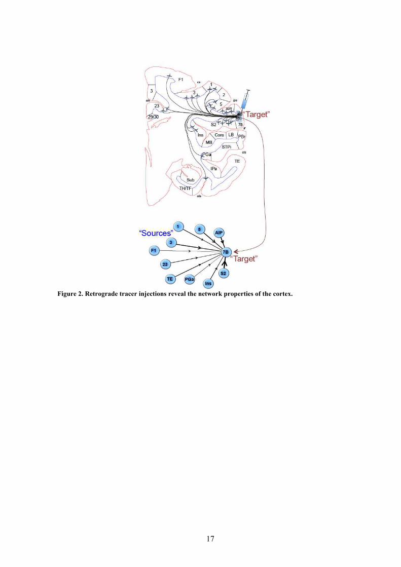
We use retrograde tracers to characterize the inter-areal network (Figure 2). In our

studies, we exploit two measures of neural connectivity (Figure 3). The Fraction of Labeled

Neurons (FLN) is the proportion of neurons that project from a cortical area (or sub-cortical

structure) to a given injection site with respect to the total number of neurons throughout the

brain that are labeled by the tracer injection. In many cases, we deal only with the connections

that are extrinsic to the area in which the injection was made. In that case, we refer to the

FLNe. The number of neurons projecting from an area can be further characterized as the

proportion that arises from the supragranular layers; this proportion we refer to as the SLN. The

SLN provides an index of the laminar signature of a projection. Here, we will only discuss the

statistics of the FLN, though some of the issues apply equally to the SLN index.

Even though the FLN and SLN are proportions, i.e., continuous values in the interval

[0, 1], the data are by origin counts of numbers of neurons, i.e., discrete and non-negative. This

feature has direct consequences on the characteristics of the data, their variability, how they are

modeled and ultimately how they are interpreted. While it is true that for large counts, the data

are likely to be well approximated by assuming normality (thanks to the Central Limit Theorem

(Wasserman, 2004)), the 6 orders of magnitude in strength that the FLN span when intrinsic

projections are included means that even for an injection that marks on average a few hundred

thousand neurons, there will be numerous small projections for which a normal assumption is

not likely to provide a reasonable description.

In most statistical models of counts, the variance depends on the mean. For example, in

the simplest case, which corresponds to the Poisson distribution, the variance equals the mean

(or equivalent, the standard deviation (SD) equals the square root of the mean). It is often the

case in real data, however, that a number of factors conspire to generate higher variances than

expected from the mean, a phenomenon called overdispersion (Hilbe, 2007). Scannell et al.

(Scannell et al., 2000) analyzed the mean-SD relation for tracer injection studies from their own

and other laboratories and concluded that the overdispersion in neural count data was

sufficiently severe to present a serious problem in the feasibility of the interpretability of

measures of connectivity strength based on neural counts.

Statisticians have devised a number of alternative models to the Poisson to take into

account and to handle overdispersion in count data. One of the simplest alternatives to the

Poisson model is the negative binomial family of models (Hilbe, 2007). The negative binomial

is derived by assuming that the mean parameter of the Poisson is not fixed but subject to

random variability described by a Gamma distribution. Thus, the negative binomial model

includes a second parameter called the dispersion that permits modeling the increased

variability over and above that expected from a Poisson distribution. Importantly, the Poisson

model arises as a limiting case in this family. Analyzing multiple injections to each of three

visual areas and one prefrontal area, we confirmed significant overdispersion in our data, as

described by Scannell et al. (Scannell et al., 2000), and found that the negative binomial

provided a good description of the variability in the data (Markov et al., 2011). Importantly, this

5

model also accurately accounted for the consistency of the weakest projections (Markov et al.,

2013b). Based on this model, the estimated confidence intervals for a projection were less than

an order of magnitude. Thus, given the 5 order of magnitude variation in projection strength for

the FLNe, we can establish a distinct connectivity profile that characterizes each area (Figures 4

and 6).

Interestingly, however, the dispersion parameter estimated for all four injection sites

was quite similar, suggesting that the factors that influence the variability in the data are

common across the four areas and by inference across the cortex (Markov et al., 2013b). The

implications of this regularity in the data are quite profound for a project aiming at

characterizing the weighted connectivity profile of the macaque brain in that it opens up the

possibility of evaluating the precision of single injections. Given the enormous effort required

to count all of the neurons from even a single injection, this represents a considerable savings in

time and puts the scope of such a project within reach.

In this way, we have been able to report connectivity profiles based on single injections

for an additional 25 cortical areas sampled across the cortex (Figure 4). These confirm another

regularity that we discovered in the original repeat injections (Markov et al., 2013b; Markov et

al., 2011) and that is that the range of strengths of the projections onto the injection site follow a

log normal distribution (Figure 5). This relation has since been confirmed as well in mouse

cortex (Wang et al., 2012).

3. Characteristics of the cortical network

The 29 injections revealed 1615 interareal pathways of which 37% had not been

reported in earlier studies and were referred to as newfound projections (NFP) and were

distinguished from the 63% known pathways (Markov et al., 2013b). The reasons why so many

connections have been missed are multiple and have been partially referred to in the section

above dealing with collated data and are discussed in detail elsewhere (Markov et al., 2013a;

Markov et al., 2013b). Real world networks are weighted and directed (Boccaletti et al., 2006)

and a major aim of our study was to capture both of these features in the inter-areal cortical

network (Markov et al., 2013b). Because we define the weight and direction of the connections

we were able to show that connections between two areas are in the vast majority of cases very

asymmetric in terms of weight. In some cases the weight in one direction was zero in contrast to

moderate to weak in the opposite direction. We found evidence for unidirectionality in 33% of

pathways; an altogether unexpected finding given that earlier studies had claimed that bi-

directionality was a characteristic feature of the cortex. However many of these claims of bi-

directionality were subsequent to the use of tracers such as horseradish peroxidase that are

carried both anterogradely and retrogradely. Given the numerical importance of intrinsic local

connections, the high incidence of anterograde labeling in these early studies could actually

reflect axon collaterals of the retrograde labeled cells, which could lead an investigator to

conclude on a bidirectional connection when the connection was in fact unidirectional.

The high 37% incidence of NFP was not in retrospect so surprising because in our

previous study we had shown that the well-studied areas V1, V2 and V4 returned 20% NFP

(Markov et al., 2011). When the weights of the NFP were examined in a recent study, they were

found to be predominantly low-weight long-distance pathways, which nevertheless had weight

distributions that overlapped extensively with known pathways (Markov et al., 2013a; Markov

et al., 2013b). In the 2013a study we set out to examine the consequence of the observed

correlation of weight and distance and how this correlation largely explains many of the

observed features of the NFP.

An important observation was that all the areas in a designated region (occipital,

parietal, temporal, frontal and prefrontal) received inputs from a subset of all the areas

projecting to that region. Inclusion of the NFP caused the percentage of common input to

increase significantly from 7 to 19%. The common input to a region constitutes a sort of

6

connectivity signature of that region and allows us to test the specificity of the connectivity via

permutation tests. In a first instance, we showed that replacing the NFP by randomly chosen

connections had a significant influence on the numbers of common input, indicating that the

NFP is a highly selective set of long-distance connections. The presence of a regional signature

makes it possible to examine if NFP and known projections contributed differently to the

signature. This amounts to comparing an aspect of the selectivity of the NFP and known

connections. This showed that both sets of connections displayed similar regional selectivity.

As graph density increases, variability within the graph becomes progressively less

significant (the complete graph has 100% density and zero variability, as there is only one such

graph). Given the high density of the cortical graph one might have expected that the NFP were

more or less random connections with little specificity. As we have seen this was not the case.

The observation that the NFP exhibited a high binary specificity (i.e. a specificity dependent

uniquely on a connection being present or absent) was surprising given the high density of the

cortical graph. Could this be related to the distance properties of the NFP? A number of studies

had observed that neighboring areas are frequently connected (Markov et al., 2011; Young et

al., 1995). This would lead to the prediction that short-distance connectivity is very similar for

neighboring areas and that this similarity falls off with distance. We introduced both a weighted

and binary defined similarity index (Markov et al., 2013a) in order to measure the effect of

distance and indeed it showed that within region similarity was high, and between region

similarity is lower, and tends to decline with distance. The similarity index measures the degree

to which two areas receive input (or avoid receiving input) from common sources or project (or

avoid projecting) to common target areas. The dissimilarity of long-distance connections means

that they could show high binary specificity. For this to be the case one would predict that

distance would have an important effect on the probability of areas being connected. We

investigated this by examining the probability of connection pairs at different distances to be

connected. At short distances the probability was 100%, and there was a steady decline in

probability to less than 10% at far distances. Hence, subgraphs of the within region connectivity

fall in the range of 90-100%, while that of the between regions have a mean density of 50%

indicating that binary specificity in the cortical graph is a unique property of long-distance

connections.

These results point to the importance of long-distance connections in shaping the

cortical graph. Are long-distance connections evenly distributed across the cortex? We were

able to show that this is not the case. When the inputs and outputs of all regions were compared

it was found that the prefrontal cortex is characterized by significantly higher in-degree and

importantly more numerous long-distance connections (Markov et al., 2013a). These highly

abundant long-distance connections of the areas of the prefrontal cortex could play a privileged

role for example in the global neuronal workspace model of consciousness (Dehaene and

Changeux, 2011; Harriger et al., 2012) (see discussion).

An injection of a target area reveals all the incoming projections (see Figure 2),

generating the network G29x91 of all the connections incoming to the 29 targets (a total of 1615

connections). Accordingly, the projections that are revealed between the injected areas only,

provide complete connectivity information within that set. The current database, with its 29

injected target areas, thus allows generating an edge-complete cortical G29x29 subgraph in which

the connectivity status between any two nodes of the G29x29 is fully known. This connectivity

status will not change with further injections. Given that the 29 areas injected are widely

distributed amongst the six regions, the availability of such an edge-complete sub-network is

crucial as many of this network’s properties are expected to scale up to the full inter-areal

network (FIN) of 91 nodes G91x91. One such property is graph density, a fundamental measure of

a network’s overall connectedness, defined as the fraction between the number of existing edges

and the maximum number of edges that it could have. For a graph with N =29 nodes the

maximum number of directed edges is N(N-1) = 812. As there were 536 directed projections

7

revealed within the set of 29 injected areas, this yields a high density of 536/812 = 0.66. That is,

of all possible connections 66% of them do exist. Assuming the same average number of

incoming links as in the 29 targets for the rest of the yet-to-be injected 62 areas, we estimate a

high density of 62% to hold for the FIN as well (Markov et al., 2013a). Additional evidence

about the high density of the FIN is provided by a dominating set analysis of the G29x91 network

(Eubank et al., 2004; Kulli and Sigarkanti, 1991; Markov et al., 2013b). A group D of nodes is

said to dominate x% of the network if x% of all the nodes form one or more links to nodes in D.

A minimum dominating set (MDS) is the smallest of such groups that fully (x%=100%)

dominates the network. A small MDS implies either a very dense network or a network

dominated by hubs. However, the in-degree distribution of G29x91 is inconsistent with that of

scale-free networks (Markov et al., 2013a; Markov et al., 2013b). We have found that a pair of

areas (8l and 7m) receives projections from all the 91 areas, revealing an extremely small MDS

size of 2. Moreover, for all sets of 2 target area combinations from the 29 target areas (406

pairs), 26.6% of them dominate 90–100% of the 91 areas. Interestingly, all combinations of 8

sites (out of 29, about 4.29 million) will dominate at least 90% of all the areas in the G29x91. As

more injections add links but not new nodes, they can only enhance these strong domination

effects, meaning that the FIN is indeed a dense graph (Markov et al., 2013a; Markov et al.,

2013b). Dominating set analysis can not only be used to confirm graph density but also as a tool

to capture and describe structural specificity, as described below.

Real world networks that have evolved to perform multiple and complex functions, and

thus networks like the cortex cannot be simple random graphs, as random, uncorrelated

structures cannot encode and process information. Hence the structure of functional complex

networks is expected to be heterogeneous, on multiple levels, indicative of the range and

complexity of their functional repertoire. Although the inter-areal level network compared to the

neuronal level network is very coarse-grained and thus constrained, structural heterogeneity

does appear, on the one hand through the 5-6 orders of magnitude variability in connection

weights (FLNe-s) and on the other, through its binary structural properties, as discussed in the

following paragraphs.

Structural specificity at the binary level would be rather surprising because at 66%

density the structure of a typical graph is constrained, and thus one would not expect significant

binary specificity. In contrast, in sparse graphs (e.g., in the social network) there is a lot more

wiggle room for edge placement and hence more possibilities for deviations from purely

random (unstructured) graphs. In the previous sections we have seen that the NFP and hence

the weak, long-range connections have highly specific roles in the network’s binary structure.

One can then ask whether the overall structure of the G29x29 subgraph shows some level of

heterogeneity (in spite of its high density). We next show that indeed, and rather surprisingly,

the overall structure of the G29x29 subgraph does have strong structural specificity. However, we

need the proper graph theoretical tools to extract this information from dense graphs.

It has been observed that many real world complex networks are heterogeneous and

possess a network “core” formed by a group of high centrality nodes, more densely

interconnected amongst themselves then with the rest of the network. The high centrality nodes

are typically identified as nodes with the largest degrees. Here we discuss two graph theoretical

algorithms used to detect such network cores and which have both been applied to cortical

networks. One is k-core decomposition (Alvarez-Hamelin et al., 2005; Seidman, 1983) and the

other is the recently introduced “rich-club” analysis (Colizza et al., 2006). Modha and Singh

(Modha and Singh, 2010) applied k-core decomposition in order to identify the core region of a

network representation of the cortex inferred from the CoCoMac dataset. The analyzed network

had 383 nodes and 5,208 undirected edges corresponding to a 7% graph density. In k-core

decomposition nodes that have degree smaller than k are recursively pruned from the graph,

until the remaining nodes have a degree of k or larger. Varying the degree threshold k, a

decomposition of the graph is obtained in the form of nested subgraphs, with higher-k

8

components embedded within the lower-k subgraphs. The innermost (highest k-value) subgraph

is then defined as the network core. Using this method Modha and Singe (2010) observed a

large innermost core of 122 vertices (31% of total) with k=29 (that is every node in the core

connected to at least 29 core nodes).

Another often-used graph theoretical measure to capture structural organization beyond

random fluctuations in order to detect a possibly network core is based on the so-called rich-

club notion. The normalized binary rich-club measure !norm(k) is given by the ratio between the

number of edges connecting nodes of a degree larger than a given threshold k and the same

measure in a graph obtained from the original after randomly rewiring its links, while

preserving its degree sequence (Colizza et al., 2006). When viewed as function of k this

measure becomes larger than unity at high enough degrees for those networks that possess a

rich-club. This method was employed by Harriger et al. (Harriger et al., 2012) on a similar

network inferred from the CoCoMac dataset as in the Modha and Singh study, also with about

7% density. These authors claimed that indeed a rich club subgraph could be identified

containing 18% of all nodes.

Although there are differences in the cores identified by the two methods, the overlap

between the outcomes of the two approaches has shown that a major portion of the network core

originates from prefrontal areas. As discussed below, both methods have shortcomings when

applied to dense graphs and in particular to G29x29.

The G29x29 has full connectivity information and therefore is not biased by missing links

within its set of 29 nodes. We have performed the rich-club analysis on this graph. As the G29x29

graph is a very dense binary graph, there are many high-degree nodes, and thus the rich-club

measure !norm(k) shows much less sensitivity than in the case of strongly degree-heterogeneous

sparse networks such as scale-free networks (for which the rich-club notion was introduced in

the first place). For this reason the rich-club analysis cannot be used reliably on the G29x29 graph.

It is also unable to extract structure within the higher density subgraphs of an already dense

graph. The k-core decomposition, which is also based on thresholding by high-degree, is

likewise unable to identify structure within dense graphs, as the “core” identified would be

formed by the majority of the nodes in the graph. Recall that even in the sparse 7% density

graph of the Modha and Singh paper, the core was formed by 31% of all nodes, already a large

fraction. Thus, one needs a novel method that is more suitable in extracting network cores from

high-density graphs and that also provides information on the internal organization of the core.

In a recent paper (Ercsey-Ravasz et al., 2013) we introduced a method based on clique

distribution analysis (Bron and Kerbosch, 1973). Cliques are small subgraphs that have all

possible connections amongst all nodes, i.e. a 100% density within the subgraph. Since there are

many more connections, in a high-density graph the clique probability is a high. Thus, the

distribution (sizes and numbers) of such cliques provides more refined information about

structural heterogeneity than methods based on degree criteria alone. In particular, we have

identified (Ercsey-Ravasz et al., 2013) a network core of 17 nodes, forming 13 cliques of size

10, with a subgraph density of 92% within the core! Since this 17-node core is part of the edge-

complete subgraph, its structure and thus its density cannot be affected by further injections.

Importantly, this implies that this core is a component of the network core for the full G91x91

graph (FIN). The occurrence of such a high density, 17-node core in a random graph with 29

nodes and 66% link density has an infinitesimally small probability of ~10-17, demonstrating the

high level of binary specificity of the cortical network. Comparing the cores identified in all

three studies discussed here (k-core, rich-club and clique) we find that the prefrontal areas

dominate all three of them, in spite of the fact that they were obtained from different levels of

representations, and different quality datasets and methods.

4. Discussion

9

4.1. Binary and weighted specificity of the cortical graph. The primary outline of our recent

studies has been to explore the specificity of the interareal cortical network (Markov et al.,

2013a; Markov et al., 2013b; Markov and Kennedy, 2013; Markov et al., 2011). The high

density of the cortical graph suggests that connectivity weight provides the major heterogeneity

of the graph allowing specificity. Overall injections reveal connection weights spanning a huge

5 to 6 orders of magnitude, while our repeat injections demonstrate that in spite of the

variability in the connection weights across animals, the weakest connections are found

consistently across individuals. Individual cortical areas receive inputs on average from 50 areas

(range 26-87) out of a total of 93 areas. The broad range of connection weights and the set of

areas together define a connectivity profile for each cortical area. The fact that the connectivity

profile of an area is consistent across brains suggests that the physiological function of an area

is constrained by its connectivity profile (Passingham et al., 2002). Earlier studies have not

systematically addressed the issue of the weight of individual pathways; this and incomplete

data leads to the poor agreement between the connectivity profile determined by CoCoMac and

our results (Figure 6).

The present study reveals a high 66% density of the cortical graph. This is in sharp

contrast to the assumptions made by numerous network models of the cortex. Further, we have

shown that modifying the granularity of the parcellation does not significantly change the

results (Markov et al., 2013b). The studies based on collated data failed to distinguish between

test absent and not tested and assumed densities of between 7% and 30% (Honey et al., 2007;

Modha and Singh, 2010; Young, 1993). The topological properties of graphs at such low

densities will be quite different from that of the cortical graph and this will be examined in a

later study. At a density of 66% it was highly unexpected to find the binary specificity of the

long distance connections that we have observed.

4.2. NFP and the role of weak connections. So far we have examined the connectivity of 29

cortical areas and found NFP to all areas including the well-studied area, area V1 or 17. There is

no single reason that explains why these connections have not been reported in earlier studies.

One likely explanation is that anatomical studies usually address the connectivity of an area in

the context of the system of which it is part. Thus an investigation of for example area V1 will

primarily be concerned by its connections to other visual areas, and may fail to address the

possibility of the primary visual area being connected to non-visual areas. This is the most

likely reason that the projections from auditory areas to area V1 were not detected before 2002

(Falchier et al., 2002; Rockland and Ojima, 2003). While these connections are considerably

weaker than those from the extrastriate areas they most likely play an important role in early

multimodal integration and mediating auditory response in area V1 in the blind (Klinge et al.,

2010). Another and related cause for so many connections being missed by earlier studies could

be the low weight of long-distance connections, so that the anatomist that does venture out of

the system in which the area he is studying is located will find mostly low weight projections

and he may well be tempted to discount such connections as being non-significant. Whatever

the cause, the consequence is that early reports on connectivity and the collated datasets that

have been drawn from them have been incomplete, heavily underestimating the long-distance

connections, for which our studies show high levels of binary specificity (Markov et al., 2013a).

Our inter-areal connectivity data show that earlier studies have had an important bias in

that they have failed to report approximately 50% of the long-distance low weight connections.

Long-distance pathways are found also to contribute low proportions of synapses (1-6%)

(Anderson et al., 1998; Anderson et al., 2011; Anderson and Martin, 2002, 2005). Do we need

to concern ourselves about these connections; after all given that they are weak one could

simply assume that in the general order of things that their contribution to the physiology of the

target area is minimal? This might be a dangerous assumption, given that there are numerous

cases of weak connections having important physiological roles. In fact connections between

hierarchical levels are invariably weak. For instance the major ascending visual input into the

10

primary visual area (area V1) is from the lateral geniculate nucleus (LGN), and lesion of the

LGN leads to loss of visual responses in the area V1 and blindness. However, the FLN values of

the LGN input to the area V1 is less than 1% (Markov et al., 2011) in agreement with the very

low (less than 10%) of the synapses in area V1 originating from the LGN.

Do the subcortical driving inputs to cortex with low FLN values have qualitatively

different structural and functional properties from cortico-cortical connections? That is in fact

the case. The synaptic morphology and the tight coupling of action potentials in geniculate

fibers partially explain the efficacy of the geniculate input compared to cortico-cortical inputs

(da Costa and Martin, 2011; Stratford et al., 1996). Likewise, there is also evidence that at least

some long-distance cortico-cortical axons have morphological features that suggest that they

may have a strong driving influence (Anderson et al., 1998). Further investigations are required

to see if there are molecular specifics of long-distance cortical connections (Bernard et al.,

2012; Hof et al., 1995; Yamamori, 2011).

There is considerable evidence in favor of wire minimization as a major adaptive

feature of the cortex (Cherniak, 1994; Cherniak et al., 1999; Cherniak et al., 2004; Chklovskii,

2000; Chklovskii and Koulakov, 2004; Chklovskii et al., 2002; Klyachko and Stevens, 2003;

Koulakov and Chklovskii, 2001; Rivera-Alba et al., 2011). This would lead to the prediction

that during brain expansion there could be reduction of numbers of connections, and the wire

minimization principal might therefore favor selective reduction in long-distance connections.

The human cortex is characterized by an important increase in dimensions so that compared to

smaller primates there could be a relative decrease in the weights of the long-distance

connections. Given the low resolution of existing brain imaging techniques one can predict that

detection of the long-distance connectivity of the human cortex will not be available for

numerous years. Meanwhile exploring the full contingent of long-distance connections in

macaque remains an important first step.

Social networks have played an important role in the evolution of network theory. An

influential paper entitled “The strength of weak ties” explored the role of the strength of social

links in sociological theory. The author argued that most network models had been concerned

principally with strong ties that are formed within small well defined groups, ignoring the weak

ties which exist between groups (Granovetter, 1983). In the social network the weak link is

thought to play a privileged role in integrating global and local structure. One can hypothesize

that weak connections in the cortex may play a similar role, serving to integrate across widely

separated regions and induce stability (Csermely, 2006).

The consistency of weak connections, their high binary specificity and ability to link

widely separated areas in the cortex raise the issue of their function. The short distance high-

weight connections would seem to have the computational power to contribute to elaborating

the receptive fields of neuron in the target areas, while the low-weight connections could

contribute to communication via oscillation perhaps by means of contraction dynamics (Fries,

2005; Wang and Slotine, 2005).

5. Conclusion.

There are a number of features of the cortical graph, some of them discussed elsewhere,

that suggest a major revision of current theories of cortical function. Perhaps the major question

is: what is the adaptive feature of the high-density graph as far as cortical computation is

concerned? One can point to phenomena such as oscillatory coherence governing

communication that may well demand such a high density (Bosman et al., 2012; Buffalo et al.,

2011; Fries, 2005). Explaining the meaning of the dense cortical graph will clearly be a

challenge for future generations of theoreticians and physiologists.

The experimental bias that underestimated the long-distance connections means that the

full connectivity of the remaining 62 areas needs to be explored. While in the papers reviewed

11

here we have mainly concentrated on the weight-distance characteristics, we also discussed

important features at the binary level as well, in particular the core-periphery organization of the

cortex at the inter-areal level. The edge-complete graph is a key notion, as its internal structure

and its properties cannot change with additional connectivity data. Using a clique analysis on

this edge-complete graph (Ercsey-Ravasz et al., 2013) we have shown the existence of a

network core of 92% density connected to a 49% density periphery. The density of connections

between core and periphery is 54%, dominated by NFP type connections (long-range). This

suggests that information distribution and integration in the brain is governed by a structurally

and functionally central circuitry, within which the connections are almost direct between any

two areas for fast and reliable signal processing.

Qualitative data of laminar patterns of inter-areal connectivity provided a much cited

and highly influential large-scale model of the hierarchy of the visual cortex (Felleman and Van

Essen, 1991). As shown in Figure 3, retrograde tracer analysis allows quantification of the

laminar distribution of the parent neurons linking cortical areas thereby providing SLN, an

index of hierarchical distance (Barone et al., 2000). Use of SLN to build cortical hierarchy

introduces important changes in the position of key areas in the hierarchy. Modern theories of

cortical function combining considerations of the physiology and anatomy of inter-areal

pathways are strongly rooted in the concept of hierarchy and predictive coding and indicate

global-local integration (Friston, 2010; Markov and Kennedy, 2013). The time is ripe to harvest

the data necessary to build a weighted and large-scale hierarchy of the inter-areal cortical

network.

Acknowledgements: P. Giroud and P. Misery for artwork and Kevan Martin for his critical

reading of the manuscript. This work was supported by FP6-2005 IST-1583 (HK); FP7-2007

ICT-216593 (HK); ANR-05-NEUR-088 (HK); LABEX CORTEX (ANR-11-LABX-0042) of

Université de Lyon, within the program "Investissements d'Avenir" (ANR-11-IDEX-0007)

operated by the French National Research Agency (ANR) (HK) and in part by HDTRA 1-09-1-

0039 (ZT).

6. References

Alvarez-Hamelin, J.I., Dall'Asta, L., Barrat, A., Vespignani, A., 2005. k-core decomposition: A

tool for the visualization of large scale networks. arXiv preprint cs/0504107.

Anderson, J.C., Binzegger, T., Martin, K.A., Rockland, K.S., 1998. The connection from

cortical area V1 to V5: a light and electron microscopic study. J Neurosci 18, 10525-

10540.

Anderson, J.C., Kennedy, H., Martin, K.A., 2011. Pathways of attention: synaptic relationships

of frontal eye field to v4, lateral intraparietal cortex, and area 46 in macaque monkey. J

Neurosci 31, 10872-10881.

Anderson, J.C., Martin, K.A., 2002. Connection from cortical area V2 to MT in macaque

monkey. J Comp Neurol 443, 56-70.

Anderson, J.C., Martin, K.A., 2005. Connection from cortical area V2 to V3A in macaque

monkey. J Comp Neurol 488, 320-330.

Bakker, R., Wachtler, T., Diesmann, M., 2012. CoCoMac 2.0 and the future of tract-tracing

databases. Frontiers in Neuroinformatics 6.

Barabasi, A.L., Albert, R., 1999. Emergence of scaling in random networks. Science 286, 509-

512.

Barone, P., Batardiere, A., Knoblauch, K., Kennedy, H., 2000. Laminar distribution of neurons

in extrastriate areas projecting to visual areas V1 and V4 correlates with the hierarchical

rank and indicates the operation of a distance rule. J Neurosci 20, 3263-3281.

12

Batardiere, A., Barone, P., Dehay, C., Kennedy, H., 1998. Area-specific laminar distribution of

cortical feedback neurons projecting to cat area 17: quantitative analysis in the adult and

during ontogeny. J Comp Neurol 396, 493-510.

Behrens, T.E., Sporns, O., 2012. Human connectomics. Curr Opin Neurobiol 22, 144-153.

Bernard, A., Lubbers, L.S., Tanis, K.Q., Luo, R., Podtelezhnikov, A.A., Finney, E.M.,

McWhorter, M.M., Serikawa, K., Lemon, T., Morgan, R., Copeland, C., Smith, K.,

Cullen, V., Davis-Turak, J., Lee, C.K., Sunkin, S.M., Loboda, A.P., Levine, D.M., Stone,

D.J., Hawrylycz, M.J., Roberts, C.J., Jones, A.R., Geschwind, D.H., Lein, E.S., 2012.

Transcriptional architecture of the primate neocortex. Neuron 73, 1083-1099.

Boccaletti, S., Latora, V., Moreno, Y., Chavez, M., Hwang, D.U., 2006. Complex networks:

structure and dynamics. Physics reports 424, 175-308.

Bosman, C.A., Schoffelen, J.M., Brunet, N., Oostenveld, R., Bastos, A.M., Womelsdorf, T.,

Rubehn, B., Stieglitz, T., De Weerd, P., Fries, P., 2012. Attentional stimulus selection

through selective synchronization between monkey visual areas. Neuron 75, 875-888.

Bron, C., Kerbosch, J., 1973. Algorithm 457: finding all cliques of an undirected graph.

Commun ACM 19, 575-577.

Buffalo, E.A., Fries, P., Landman, R., Buschman, T.J., Desimone, R., 2011. Laminar

differences in gamma and alpha coherence in the ventral stream. Proc Natl Acad Sci U S

A 108, 11262-11267.

Bullmore, E., Sporns, O., 2012. The economy of brain network organization. Nat Rev Neurosci

13, 336-349.

Cherniak, C., 1994. Component placement optimization in the brain. J Neurosci 14, 2418-2427.

Cherniak, C., Changizi, M., Won Kang, D., 1999. Large-scale optimization of neuron arbors.

Phys Rev E Stat Phys Plasmas Fluids Relat Interdiscip Topics 59, 6001-6009.

Cherniak, C., Mokhtarzada, Z., Rodriguez-Esteban, R., Changizi, K., 2004. Global optimization

of cerebral cortex layout. Proc Natl Acad Sci U S A, 101, 1081-1086

Chklovskii, D.B., 2000. Optimal sizes of dendritic and axonal arbors in a topographic

projection. J Neurophysiol 83, 2113-2119.

Chklovskii, D.B., Koulakov, A.A., 2004. Maps in the brain: what can we learn from them?

Annu Rev Neurosci 27, 369-392.

Chklovskii, D.B., Schikorski, T., Stevens, C.F., 2002. Wiring optimization in cortical circuits.

Neuron 34, 341-347.

Colizza, V., Flammini, A., Serrano, M.A., Vespignani, A., 2006. Detecting rich-club ordering in

complex networks. Nature Physics 2, 110-115.

Csermely, P., 2006. Weak Links: Stabilizers of complex systems from protein to social

networks. Springer, Berlin.

da Costa, N.M., Martin, K.A., 2011. How thalamus connects to spiny stellate cells in the cat's

visual cortex. J Neurosci 31, 2925-2937.

da Costa, N.M., Martin, K.A., 2013. Sparse reconstruction of brain circuits: or, how to survive

without a microscopic connectome. Neuroimage in this issue.

Dehaene, S., Changeux, J.P., 2011. Experimental and theoretical approaches to conscious

processing. Neuron 70, 200-227.

Ercsey-Ravasz, M., Markov, N.T., Lamy, C., Van Essen, D.C., Knoblauch, K., Toroczkai, Z.,

Kennedy, H., 2013. Connection weight heterogeneity and a distance law specify cortical

architecture. Neuron submitted.

Eubank, S., Guclu, H., Kumar, V.S., Marathe, M.V., Srinivasan, A., Toroczkai, Z., Wang, N.,

2004. Modelling disease outbreaks in realistic urban social networks. Nature 429, 180-

184.

Falchier, A., Clavagnier, S., Barone, P., Kennedy, H., 2002. Anatomical evidence of

multimodal integration in primate striate cortex. J Neurosci 22, 5749-5759.

Felleman, D.J., Van Essen, D.C., 1991. Distributed hierarchical processing in the primate

cerebral cortex. Cereb Cortex 1, 1-47.

13

Fries, P., 2005. A mechanism for cognitive dynamics: neuronal communication through

neuronal coherence. Trends Cogn Sci 9, 474-480.

Friston, K., 2010. The free-energy principle: a unified brain theory? Nat Rev Neurosci 11, 127-

138.

Gould, S.J., 1991. Wonderful Life: The Burgess Shale and the Nature of History. Norton, W.

W. and Co, New York.

Granovetter, M., 1983. The strength of weak ties: a network theory revisited. Sociological

theory, New York, pp. 201-233.

Hagmann, P., Cammoun, L., Gigandet, X., Meuli, R., Honey, C.J., Wedeen, V.J., Sporns, O.,

2008. Mapping the Structural Core of Human Cerebral Cortex. PLoS Biol 6, e159.

Harriger, L., van den Heuvel, M.P., Sporns, O., 2012. Rich club organization of macaque

cerebral cortex and its role in network communication. PLoS One 7, e46497.

Hilbe, J.M., 2007. Negative Binomial Regression. Cambridge University Press, Cambridge.

Hof, P.R., Nimchinsky, E.A., Morrison, J.H., 1995. Neurochemical phenotype of corticocortical

connections in the macaque monkey: quantitative analysis of a subset of neurofilament

protein- immunoreactive projection neurons in frontal, parietal, temporal, and cingulate

cortices. J Comp Neurol 362, 109-133.

Honey, C.J., Kotter, R., Breakspear, M., Sporns, O., 2007. Network structure of cerebral cortex

shapes functional connectivity on multiple time scales. Proc Natl Acad Sci U S A 104,

10240-10245.

Judson, H.F., 1996. The Eighth Day of Creation: Makers of the Revolution in Biology. Cold

Spring Harbor Laboratory Press.

Kennedy, H., Martin, K.A., Orban, G.A., Whitteridge, D., 1985. Receptive field properties of

neurones in visual area 1 and visual area 2 in the baboon. Neuroscience 14, 405-415.

Klinge, C., Eippert, F., Roder, B., Buchel, C., 2010. Corticocortical connections mediate

primary visual cortex responses to auditory stimulation in the blind. J Neurosci 30,

12798-12805.

Klyachko, V.A., Stevens, C.F., 2003. Connectivity optimization and the positioning of cortical

areas. Proc Natl Acad Sci U S A 100, 7937-7941.

Kotter, R., 2004. Online retrieval, processing, and visualization of primate connectivity data

from the CoCoMac database. Neuroinformatics 2, 127-144.

Koulakov, A.A., Chklovskii, D.B., 2001. Orientation preference patterns in mammalian visual

cortex: a wire length minimization approach. Neuron 29, 519-527.

Krumnack, A., Reid, A.T., Wanke, E., Bezgin, G., Kotter, R., 2010. Criteria for optimizing

cortical hierarchies with continuous ranges. Front Neuroinform 4, 7.

Kulli, V.R., Sigarkanti, S.C., 1991. Inverse domination in graphs. Nat Acad Sci Letters 14, 473-

475.

Lewis, J.W., Van Essen, D.C., 2000. Mapping of architectonic subdivisions in the macaque

monkey, with emphasis on parieto-occipital cortex. J Comp Neurol 428, 79-111.

Markov, N.T., Ercsey-Ravasz, M.M., Lamy, C., Ribeiro Gomes, A.R., Magrou, L., Misery, P.,

Giroud, P., Barone, P., Dehay, C., Toroczkai, Z., Knoblauch, K., Van Essen, D.C.,

Kennedy, H., 2013a. The role of long-range connections on the specificity of the

macaque interareal cortical network. Proc Nat Acad Sci USA 110, 5187-5192.

Markov, N.T., Ercsey-Ravasz, M.M., Ribeiro Gomes, A.R., Lamy, C., Magrou, L., Vezoli, J.,

Misery, P., Falchier, A., Quilodran, R., Gariel, M.A., Sallet, J., Gamanut, R., Huissoud,

C., Clavagnier, S., Giroud, P., Sappey-Marinier, D., Barone, P., Dehay, C., Toroczkai, Z.,

Knoblauch, K., Van Essen, D.C., Kennedy, H., 2013b. A weighted and directed interareal

connectivity matrix for macaque cerebral cortex. Cereb Cortex, DOI:

10.1093/cercor/bhs1270.

Markov, N.T., Kennedy, H., 2013. The importance of being hierarchical. Curr Opin Neurobiol

23, http://dx.doi.org/10.1016/j.conb.2012.1012.1008.

Markov, N.T., Misery, P., Falchier, A., Lamy, C., Vezoli, J., Quilodran, R., Gariel, M.A.,

Giroud, P., Ercsey-Ravasz, M., Pilaz, L.J., Huissoud, C., Barone, P., Dehay, C.,

14

Toroczkai, Z., Van Essen, D.C., Kennedy, H., Knoblauch, K., 2011. Weight Consistency

Specifies Regularities of Macaque Cortical Networks. Cereb Cortex 21, 1254-1272.

Markov, N.T., Vezoli, J., Chameau, P., Falchier, A., Quilodran, R., Huissoud, C., Lamy, C.,

Misery, P., Giroud, P., Ullman, S., Barone, P., Dehay, C., Knoblauch, K., Kennedy, H.,

2013c. The Anatomy of Hierarchy: Feedforward and feedback pathways in macaque

visual cortex. J Comp Neurol under review.

Modha, D.S., Singh, R., 2010. Network architecture of the long-distance pathways in the

macaque brain. Proc Natl Acad Sci U S A 107, 13485-13490.

Newman, M.E.J., 2010. Networks: an introduction. Oxford University Press.

Orban, G.A., Kennedy, H., Maes, H., 1980. Functional changes across the 17-18 border in the

cat. Exp Brain Res 39, 177-186.

Passingham, R.E., Stephan, K.E., Kotter, R., 2002. The anatomical basis of functional

localization in the cortex. Nat Rev Neurosci 3, 606-616.

Rivera-Alba, M., Vitaladevuni, S.N., Mishchenko, Y., Lu, Z., Takemura, S.Y., Scheffer, L.,

Meinertzhagen, I.A., Chklovskii, D.B., de Polavieja, G.G., 2011. Wiring economy and

volume exclusion determine neuronal placement in the Drosophila brain. Curr Biol 21,

2000-2005.

Rockland, K.S., Ojima, H., 2003. Multisensory convergence in calcarine visual areas in

macaque monkey. Int J Psychophysiol 50, 19-26.

Rockland, K.S., Pandya, D.N., 1979. Laminar origins and terminations of cortical connections

of the occipital lobe in the rhesus monkey. Brain Res 179, 3-20.

Scannell, J.W., Grant, S., Payne, B.R., Baddeley, R., 2000. On variability in the density of

corticocortical and thalamocortical connections. Philos Trans R Soc Lond B Biol Sci 355,

21-35.

Seidman, S.B., 1983. Network structure and minimum degree. Soc Networks 5, 269-287.

Sporns, O., 2011. Networks of the brain. MIT Press, Cambridge, Mass.

Sporns, O., Zwi, J.D., 2004. The small world of the cerebral cortex. Neuroinformatics 2, 145-

162.

Stephan, K.E., Kamper, L., Bozkurt, A., Burns, G.A., Young, M.P., Kotter, R., 2001. Advanced

database methodology for the Collation of Connectivity data on the Macaque brain

(CoCoMac). Philos Trans R Soc Lond B Biol Sci 356, 1159-1186.

Stratford, K.J., Tarczy-Hornoch, K., Martin, K.A.C., Bannister, N.J., Jack, J.J.B., 1996.

Excitatory Synaptic Inputs to Spiny Stellate Cells in Cat Visual Cortex. Nature 382, 258-

261.

Van Essen, D.C., Glasser, M.F., Dierker, D., Harwell, J., 2012a. Cortical Parcellations of the

macaque monkey analyzed on surface-based atlases. Cereb Cortex 22, 2227-2240.

Van Essen, D.C., Ugurbil, K., 2012. The future of the human connectome. Neuroimage 62,

1299-1310.

Van Essen, D.C., Ugurbil, K., Auerbach, E., Barch, D., Behrens, T.E.J., Bucholz, R., Chang, A.,

Chen, L., Corbetta, M., Curtiss, S.W., Della Penna, S., Feinberg, D., Glasser, M.F., Harel,

N., Heath, A.C., Larson-Prior, L., Marcus, D., Michalareas, G., Moeller, S., Oostenveld,

R., Petersen, S.E., Prior, F., Schlaggar, B.L., Smith, S.M., Snyder, A.Z., Xu, J., Yacoub,

E., 2012b. The Human Connectome Project: A data acquisition prospective. Neuroimage

62, 2222-2231.

Vezoli, J., Falchier, A., Jouve, B., Knoblauch, K., Young, M., Kennedy, H., 2004. Quantitative

analysis of connectivity in the visual cortex: extracting function from structure.

Neuroscientist 10, 476-482.

Wang, Q., Sporns, O., Burkhalter, A., 2012. Network analysis of corticocortical connections

reveals ventral and dorsal processing streams in mouse visual cortex. J Neurosci 32,

4386-4399.

Wang, W., Slotine, J.J., 2005. On partial contraction analysis for coupled nonlinear oscillators.

Biol Cybern 92, 38-53.

15

Wasserman, L., 2004. All of statistics: A concise course in statistical inference. Springer, New

York.

Watts, D.J., Strogatz, S.H., 1998. Collective dynamics of 'small-world' networks. Nature 393,

440-442.

Yamamori, T., 2011. Selective gene expression in regions of primate neocortex: Implications

for cortical specialization. Prog Neurobiol 94, 201-222.

Young, M.P., 1993. The organization of neural systems in the primate cerebral cortex. Proc R

Soc Lond B Biol Sci 252, 13-18.

Young, M.P., Scannell, J.W., O'Neill, M.A., Hilgetag, C.C., Burns, G., Blakemore, C., 1995.

Non-metric multidimensional scaling in the analysis of neuroanatomical connection data

and the organization of the primate cortical visual system. Philos Trans R Soc Lond B

Biol Sci 348, 281-308.

16

7. Figure legends

Figure 1. Influence of the plane of section on the parcellation of the cortex. On the left hand side is a

coronal section in the prefrontal cortex, right hand side virtual horizontal sections taken at the levels H1

to H4, the location of the coronal sections is indicated by C1. Electrode physiological recordings going

across areal borders reveal receptive fields with transitional features (Kennedy et al., 1985; Orban et al.,

1980). Because of the 3D curvature of the cortex, an areal border that appears perpendicular to the surface

as in area 11 and 12 border in the left hand coronal section, will give rise to a transition zone if the brain

is cut in a horizontal plane (right hand sections). In this transition zone (see sections H2 and H3) the

supragranular layers will be histological area 12, while the infragranular layers will be histological areas

11 and 13. Note the presence of an island of area 13 bounded by areas 11 and 12 in section H3. Here we

are illustrating how planes of section reveal border regions. In the example given the parcellation has

been made in the coronal sections, when the areas are re-examined in the horizontal plane border regions

become apparent. Most published atlases and studies make only rare mention of these transitional border

regions, a noteworthy exception being the study of Lewis and Van Essen (Lewis and Van Essen, 2000).

C1

12

C1

11

H1

H2

C1

12

11

H3

C1

1211

C1

11

H4

12

13

13

area 11

area 12

area 13

17

Figure 2. Retrograde tracer injections reveal the network properties of the cortex.

18

Figure 3: Quantitative parameters characterizing the hierarchy. A: The laminar distribution of the

retrogradely labeled parent neurons in each pathway, referred to as SLN (fraction of supragranular

neurons) is determined by high frequency sampling and quantitative analysis of labeling. Supra- and

infragranular layer neurons contribute to both feedback and feedforward pathways, but the two directions

differ by their laminar pattern. For a given injection there is a gradient of SLN of the labeled areas,

between purely FF (SLN = 100%, all the parent neurons are in the supragranular layers) to purely FB

(SLN = 0%, all the parent neurons in the infragranular layers) and all the spectrum of intermediate

connections; B: All labeled areas can then be ordered by decreasing SLN values and, at least in the early

visual areas, this order is largely consistent the with hierarchical rank order according to Felleman and

Van Essen (Markov et al., 2013c). SLN is thus used as an indicator of hierarchical distance between areas

from the same injection (Barone et al., 2000; Krumnack et al., 2010; Vezoli et al., 2004); C: FLN

(fraction of labeled neurons) indicates the relative strength of each pathway (in number of labeled

neurons) compared to the total number of neurons that are labeled in the brain after the injection. It

requires counting labeled neurons on the sections spanning the whole hemisphere, and gives insight into

the weight of connections. Vezoli et al. (Vezoli et al., 2004) showed that short-distance connections have

high FLN values, whereas the strength of connection decreases as physical distance between source and

target areas increases. D: FLN gives the proportion of labeled neurons in a given source structure after

injection in a target area. 90% of the cortical connections are restricted to the target area and correspond

to the intrinsic connections making up the local connectivity (Markov et al., 2011). If the intrinsic

connections are excluded from the calculation then the index is referred to as the FLNe.

19

Figure 4. Ordered FLNe values for one injection in cortical area V1 with expected 95% confidence

intervals (error bars) based on negative binomial model of variability. The white points indicate

ordered FLNe values for a given injection. The blue points show geometric means from all five injections

to the same area and the black points indicate the FLN values obtained from the other four injections. For

the two entries on the far right (areas STPr and 8r), there were no labelled neurons for 3 and 4 of the 5

injections. The analysis of graphs like this one indicate how accurately FLNe values from a single

injection can predict the mean obtained from multiple injections and the range of values that will be

encountered with repeat injections. These findings demonstrate that with high frequency sampling a

single retrograde injection can successfully reveal the connectivity profile of a cortical area.

Figure 5. Log FLNe values from injections of retrograde tracers in 29 cortical areas plotted against the

theoretical probabilities (inverse quantiles) of the order statistics for a normal distribution. For each of

the 29 injections, the log FLNe values were centered with respect to their means and normalized by their

standard deviation. The orange curve is the theoretical prediction if the FLNe strengths follow a log

normal distribution.

MT

TEO

FST

TH/TF

TEOm

V4t

TEa/mp

STPc

PERI

DP

IPa

STPi

8l

LB

TPt

CORE 8r

V2

V4

TEpv

MST

TEpd

V3A

V3

TEav

LIP

PGa

TEad

7op

TEa/ma

PIP

PBc

MB

STPr

M88RH

FLNe

10-5

10-4

10-3

10-2

10-1

1

0.0 0.2 0.4 0.6 0.8 1.0

-3-2

-10

12

3

Theoretical Probabilities

Ce

nte

red

an

d S

ca

led

lo

g1

0(F

LN

e)

20

Figure 6. Comparison of connectivity profiles of area F5 obtained from a collated data base

(CoCoMac) and from the consistent database of Markov et al., 2013b. A shows the connectivity

profile of area F5 reported in Markov et al., 2013b. Vertical lines indicate the 95% confidence interval

following the negative binomial model. Red stars indicate the areas used in the connectivity profile

reported in C; B is derived from Passingham et al., (2002) which used data from the CoCoMac data base;

C uses data from Markov et al., 2013b. On B connectivity profile the scales are non quantitative and

correspond to weak, medium and strong. On C, the scale is logarithmic. This figure shows the danger of

characterizing the connectivity of an areas without the knowledge of the full complement of areas

projecting to the target area, as revealed by the fact that the areas illustrated in C correspond to only a

small selection of the areas that actually project to area 5 and the diagram fails to include all of the

strongest areas. The comparison of the data from Markov et al., 2013b and Passingham et al., 2002 in

panel C shows the inadequacy of representing strength of connections extracted from incomplete and

non-quantitative data.

0

1

2

3

F1

F2

F3

F4F5

F6

F7

F1

F2

F3

F4F5

F6

F7

-5

-4

-3

-2

-1

0

B C

2S

IIF

3 32

4c

INS

U F1

44 1 8l

24

d 8r

23

24

bE

NT

O4

6v

TE

pv

10

PE

RI

V1

TE

MP 9

8m

TE

pd

MB 32

V2

F6

SU

BI

Pi

V6

A2

9/3

0V

6V

37

m 25

�

�

���

�

�� �

� ������ �

�

���

�

� �

� � � ��

��

��

Area F5

Lo

g (

FL

Ne

)

−6

−4

−2

0

F4

7B

Pro

M1

2G

uO

PR

OLIP

AIP

9/4

6v

F2

24

aO

PA

I1

14

5B

TE

av

13

5 46

d7

AT

Ea/m

aC

OR

EL

B8

BS

TP

rT

Ea/m

pP

Br

F7

7o

p9

/46

d4

5A

ST

Pi

TE

Om

14

TH

/TF

MIP

ST

Pc

* ** * **

A