Why Derivatives on Derivatives? The Case of Spread Futures Charles J. Cuny Texas A&M University College Station, TX 77843-4218 (979) 845-3656 [email protected]November 2003 I thank the Chicago Board of Trade (Market Data Products and Information Department) for providing data.
Transcript
Why Derivatives on Derivatives? The Case of Spread Futures
In January 2001, Alliance/CBOT/Eurex (a/c/e), a joint venture of the Chicago Board of
Trade and Eurex futures exchanges, began trading four separate reduced tick spread
futures contracts. These futures contracts are traded exclusively on the a/c/e electronic
trading platform, while their clearing is through the CBOT system. The underlying asset
for these futures is a calendar spread position across two otherwise identical CBOT
futures contracts with adjacent delivery dates. Thus, these spread futures contracts are
redundant securities in the sense that the contract essentially consists of a long position in
one futures contract, and a short position in another futures contract, with the two legs of
the spread differing only in their delivery dates.
For example, the March 10-year US Treasury Note Futures Reduced Tick Spread
futures contract has a trading unit that consists of “one March-June Ten-year US
Treasury Note futures spread having a face value at maturity of $100,000 or multiple
thereof”1. Taking a long position in this spread futures contract immediately gives the
trader a long position in the CBOT June 10-year US Treasury Note futures, and a short
position in the CBOT March 10-year US Treasury Note futures, just as if these two
positions were entered into directly, but separately, through the CBOT Treasury Note
futures markets. Thus, for clearing purposes, a trade executed in a spread futures contract
is recognized as being exactly the same as two trades in the futures contracts
corresponding to the legs of the calendar spread.
In another, narrower sense, reduced tick spread futures contracts are perhaps not
totally redundant: although the tick size of the CBOT Mar 10-Year US Treasury Note
futures contract is one-half of 1/32 of a point, the tick size of the associated a/c/e
Reduced Tick Spread futures contract is, as implied by its name, smaller: one-quarter of
1/32 of a point.2 Thus, reduced tick spread futures can trade at prices unavailable by
taking the associated direct long and short positions in the underlying futures markets.3
1 Language taken from the description on the Chicago Board of Trade website www.cbot.com 2 The tick size for the CBOT Treasury note (both 10-year and 5-year) and Agency note (both 10-year and 5-year) futures contracts is one-half of 1/32 of one point. The tick size for the CBOT Treasury bond and Interest rate swap (both 10-year and 5-year) futures contracts is 1/32 of one point. The tick size of all the associated reduced tick spread futures is one-quarter of 1/32 of one point. Thus, the tick size for each spread futures contract is one-half or one-quarter the tick size of the associated futures contracts. 3 Of course, if reducing the tick size is the primary innovation associated with these spread futures, one could ask why not instead reduce the tick size on the underlying CBOT futures contracts.
1
Because the spread futures contract price reflects the price differential between
two futures contracts (differing in delivery date), one would naturally expect the spread
futures price to be much smaller than the price of either leg of the underlying spread. In
light of this, implementing the reduced tick pricing may seem quite natural. Furthermore,
the spread differential may even carry a negative price, depending upon the slope of the
interest-rate term structure, for the case of interest-rate futures.4
However, since spread futures contracts are redundant, in the sense that the
underlying spread could be straightforwardly traded on other futures markets, it is not
immediately clear why this particular financial innovation should be successful. Indeed,
not only are spread futures contracts a derivative of another derivative (that is, the two
underlying futures contracts composing the calendar spread), but the particular spread
futures introduced to date are based on very liquid futures contracts. This paper examines
how the introduction of this apparently redundant security can nevertheless change the
trading behavior and welfare of hedgers in such a way as to make this innovation
potentially attractive to a futures exchange.
As of now, a/c/e has introduced seven reduced tick spread futures contracts. Three
of these, with underlying of US Treasury Bond futures, 10-year Treasury Note futures,
and 5-year Treasury Note futures, were introduced in January 2001, and have been well
received in the marketplace. A 10-year Agency Note futures reduced tick spread futures
contract was also introduced in January 2001. Although modestly successful at first,5 the
trading volume for both the underlying 10-year Agency Note futures and its associated
reduced tick spread futures have migrated to the 10-year Swap futures and its associated
reduced tick spread futures since the CBOT introduced the 10-year Swap futures contract
in October 2001 (followed by its reduced tick spread futures contract in May 2002). Two
other reduced tick spread futures products, based on the 5-year Agency Note futures and
5-year Swap futures contracts, have also been introduced. However, neither of the two
underlying futures contracts nor their associated reduced tick spread futures contracts
4 a/c/e has developed a pricing convention responding to traders’ presumed disinclination to work with negative prices. The convention is based on adding 100 basis points to the price differential for all reduced tick spread futures prices. 5 The underlying 10-year Agency Note futures contract has also achieved only modest success since its introduction in 2000.
2
have ever generated meaningful volume up to this time. Figure 1 shows the monthly
trading volume to date for the first five reduced tick spread futures contracts.
As is apparent from Figure 1, there is seasonality in the volume for each of these
contracts. The expiration month on all the underlying financial futures contracts is
March, June, September, or December. The significant demand for rolling over futures
contracts occurs in four weeks leading up to the contract expiration date. Closer
examination of daily trading volume reveals that, for each of these reduced tick spread
futures, volume starts to visibly increase around the 15th to 20th of the previous month,
typically peaks on the 28th or 29th, then visibly decreases around the 7th of the contract
month. (For example, for the March contract, the largest volume occurs from about
February 15 through March 7.)
This paper shows how the structure of the transaction costs (modeled in the form
of bid-ask spreads) in the futures market is changed by the introduction of calendar
spread futures. The futures markets exist in the model to service hedging demand, an
approach traceable to Working (1953). Also present are informed traders. Market-makers
provide liquidity to the market, which is costly to provide due to the adverse selection of
facing informed traders. Market-makers are compensated for this through charging
traders a bid-ask spread. With competitive market-makers, bid-ask spreads in each
contract are set to just cover the adverse selection faced by market-makers in that
contract. However, if the cost of trading a calendar spread is lower in the spread futures
than the primary futures market, then hedgers' trades will partially migrate to the spread
futures market, leaving informed trading in the primary market. Furthermore, if the
overall cost of implementing hedging trades falls, additional hedging interest may arise in
the primary market.
Introducing spread futures allows partial separation of hedging and informed
trading. Trading in the spread futures market is concentrated in hedging, and therefore
supports a lower bid-ask spread. To implement this requires offering a finer pricing
structure, or a reduced tick size, in the spread futures relative to the primary futures
market.
A similar result may be obtained if bid-ask spreads are set by an exchange
exercising pricing power in order to maximize aggregate market-maker profit. With these
3
"monopolistic" bid-ask spreads, it is optimal to lower the bid-ask spread in the calendar
spread futures, attracting hedgers, while raising the bid-ask spread in the primary market.
This allows price discrimination between hedgers and informed traders. Informed traders
face higher costs of trading, and reduce their activity, moderating the adverse selection
problem faced by the market-makers. The lower bid-ask spread in the spread futures
market effectively subsidizes hedgers, keeping their overall trading cost relatively low in
order to generate the hedging trade activity that market-makers find profitable. Since
hedgers have the opportunity to adjust their trading to respond to the new trading cost
structure, there will be a movement toward markets featuring relatively lower trading
costs. In particular, since spreading is now more cost effective, hedgers are more willing
to enter into initial positions that may require a later portfolio adjustment utilizing spread
futures. This trading adjustment allows for a decrease in the aggregate cost of trading
borne by the hedgers.
An important factor in the implementation of either such equilibrium, offering a
lower bid-ask spread for direct trading of the calendar spread, is that the spread futures
contract trades with a smaller tick size than the primary futures market. Even without the
presence of the spread futures, a trader could, in principle, negotiate both legs of the
calendar spread simultaneously in the futures market. However, the possible prices at
which the legs can be negotiated is constrained by the tick size. By allowing a smaller
tick size, the presence of the spread futures market allows a finer set of possible prices,
and therefore a smaller bid-ask spread (lower transaction cost) in trading the calendar
spread.
Excellent overviews of the literature on financial innovation are provided in Allen
and Gale (1994) and Duffie and Rahi (1995). Specific cases of innovations of futures
contracts are discussed in Working (1953), Gray (1970), Sandor (1973), Silber (1981),
and Johnston and McConnell (1989).
This paper reaches the conclusion that the introduction of spread futures, which
appear to be a redundant security, can change trading patterns and hedger welfare. In the
options literature, there is evidence that options may not be truly redundant. Conrad
the introduction of stock option trading for listings from 1974 and 1980. Detemple and
4
Jorion (1990) find similar abnormal stock returns for listings from 1973 to 1982, but no
significant effect for listings from 1982 to 1986. Back (1993) models a market where an
option can be synthesized via dynamic trading, thus appearing to be redundant, but the
option's existence affects the information flow, making the underlying asset volatility
stochastic. Longstaff (1995), for the case of S&P 100 index options, rejects the
martingale restriction that the value of the underlying asset implied by the cross-section
of options prices equals its actual market value, finding that the differences in value is
related to market frictions. If markets are dynamically complete and options are
redundant assets, then any option payoff can be replicated using the underlying asset and
one additional option. Buraschi and Jackwerth (2001) perform this direct test, concluding
that at-the-money S&P 500 index options and the underlying index do not span the
pricing space; consequently, the options are not redundant securities. Bakshi, Cao, and
Chen (2000) conclude that index options are not redundant assets, as the index level and
associated call option prices often move in opposite directions.
There is also a literature on how the introduction of futures contracts may affect
the underlying asset markets. A comprehensive summary of this literature is in Mayhew
(2000). One related paper is Subrahmanyam (1991), which provides an information-
based model for stock-index futures (“basket trading”), extending Kyle’s (1984) model to
allow simultaneous trading of individual stocks and baskets of stocks. With the
introduction of trading the basket, uninformed traders tend to trade the basket to protect
themselves from the informed traders who tend to trade individual stocks. (The informed
traders have stock-specific information.) Thus, the model predicts liquidity will migrate
from the markets for individual stocks to the basket.
1. The model The model contains hedgers, informed traders, and market-makers in an overlapping
generations-style marketplace. Market-makers provide liquidity to the futures markets by
taking the opposite side of trades, as needed, and are compensated by capturing the
difference between the bid and ask prices. The cost faced by market-makers is the
adverse selection cost incurred when trading against better informed traders. Market-
makers are risk neutral.
5
Time is broken up into a series of trading periods (dates). There is a risky asset,
whose underlying value changes between each period, with mean zero and variance σ2
(value changes are independent over time). A series of futures contracts are available,
each of which is tradable for two consecutive periods, after which delivery takes place
(although in our model, traders clear their positions before delivery occurs). Futures
contracts overlap, so that in each trading period, two futures contracts with different
delivery dates are extant: traders can take positions in the "new" contract (delivery
immediately after next period), and close out positions in the "old" contract (delivery
immediately after this period).
Each period, there is a mass H of new hedgers. Each hedger is equally likely to be
endowed with +E or –E units of the risky asset. Each hedger’s lifetime is either one
period long (a fraction 1 – q of the hedgers) or two periods long (fraction q). A hedger
can trade in the futures market(s) for the risky asset during his life. Thus, a hedger with a
one period lifetime born at date T can initiate a futures position at date T, and close the
position at date T + 1, while a hedger with a two period lifetime can initiate a futures
position at date T, adjust it at date T + 1, and close it at date T + 2. Hedgers do not know
their lifetime at birth, but find it out after one period passes. Hedgers consume during
their final period of life, and have mean-variance utility with risk-aversion Γ over final
consumption.
Each period, there is a mass I of new informed traders. Each informed trader has
private information about the next periodic change in the value of the risky asset.
Conditional on her information, an informed trader either appraises the next risky asset
value change as having mean +θ > 0 or mean –θ (equally likely, ex ante), with variance
kσ2. Therefore, an informed trader's gain from making a unit trade (of appropriate
direction) in the risky asset has mean θ and variance kσ2 (less bid-ask spread).6 The
parameters θ and k thus measure the mean and variance of the quality of informed
6 One possible underlying structure is that the underlying risky asset value change is equally likely to be +σ or -σ each period, and the informed trader, after observing her signal, assigns probability p > 1/2 to the correct direction of price movement. Then θ = pσ - (1 - p)σ = (2p - 1)σ, and k = 4p(1 - p). Another possible underlying structure is that the asset value change each period takes the form Θ + Φ, with Θ equally likely to be +θ or -θ, and Φ independent of Θ. If the informed perfectly observes Θ, then k = 1 - (θ/σ)2.
6
traders’ information. Informed traders have one period lifetimes, consume during their
final period of life, and have mean-variance utility with risk-aversion Γ over final
consumption.
Two scenarios are considered: a scenario with the two already described futures
contracts, new and old, trading each period (“without spread futures”), and an alternative
scenario with a spread futures contract available as well (“with spread futures”). The
available spread futures contract is based on the calendar spread between the new and old
contracts, and is identical to a long position in the new contract combined with a short
position in the old contract. The spread futures contract, when available to trade, will be
the natural instrument for hedgers who discover their lifespan is two periods, leading to a
desire to roll over their short-lived position into a longer-lived position. Utilizing spread
futures allows these hedgers to convert their position in the old contract (which delivers
before the conclusion of their hedging needs) into a position in the new contract (which
delivers after the conclusion of their hedging needs). Of course, if the spread futures
contract is unavailable, the hedgers can achieve a similar result directly by
simultaneously trading equal and opposite positions in the new and old futures contracts.
Market-makers receive (and traders incur) a bid-ask spread in trading. The bid-
ask spread is the frictional cost associated with a round trip trade for a hedger or
informed trader. The endogenously determined bid-ask spread in the futures for the risky
asset is denoted by S. When the spread futures are available, the bid-ask spread in the
spread futures is denoted by D. Since the calendar spread can always be directly created
in the futures markets, D ≤ S.
Suppose that spread futures are available to trade. A hedger with endowment –E
optimally takes an initial futures position x(S, D) satisfying7
Max (1 – q)[– S|x| – Γσ2(x – E)2/2] + q[–(S + D)|x| – 2Γσ2(x – E)2/2]. (1) x
7 Although it is possible that a long-lived hedger will want to adjust his futures position after one period has passed, it is straightforward to show that an optimal multiperiod hedge holds the same futures position after each period. Thus, a long-lived hedger simply rolls over the entire position to the next period.
7
This initial position is non-negative, x(S, D) ≥ 0, and is thus a long position.
Symmetrically, for a hedger with endowment +E, the optimal initial futures position is
-x(S, D), a short position of identical magnitude. Therefore, all H hedgers take an initial
futures position with magnitude x(S, D). Of these hedgers, qH will be long-lived and roll
over their position next period using spread futures, while (1 - q)H will be short-lived and
simply close their position next period.
An informed trader with conditional mean +θ optimally takes futures position
y(S) satisfying
Max (θ – S)y – Γkσ2 y2/2 (2) y
if S ≤ θ. If the bid-ask spread is so large that S > θ, then informed traders do not
participate in the market, y(S) = 0. Similarly, an informed trader with conditional mean –
θ optimally takes futures position -y(S). Thus, y(S) is the magnitude of the futures
position for all I informed traders.
Alternatively, suppose that spread futures contracts are not available for trade.
The same calendar spread trade can be made directly by trading in the underlying futures
contracts, albeit with a different frictional cost, a bid-ask spread of S. The trades of both
hedgers and informed can be inferred by setting D = S in the previous analysis. All H
hedgers take an initial futures position with magnitude x(S, S). All hedgers will close this
position next period, but qH of the hedgers will also open the same size position in the
subsequent delivery futures contract. As before, all I informed traders take an initial
position of magnitude y(S).
2. Competitive bid-ask spreads This section considers the case of the bid-ask spread(s) for futures contracts being set
competitively. Thus, the bid-ask spread is set so that market-makers break even in
expectation. In the absence of spread futures, the breakeven condition in the primary
futures market is
8
0 = H(1 + q)S · x(S, S) + I(S – θ) · y(S). (3)
Here, H hedgers generate trade volume H(1 + q) · x(S, S); market-makers receive the bid-
ask spread S per contract traded. I informed traders generate volume I · y(S); market-
makers receive the bid-ask spread S but expect to lose θ per contract traded due to
information asymmetry. In the absence of spread futures, denote the competitive bid-ask
spread in the primary futures market, satisfying (3), by SNSF.
In the presence of spread futures, the breakeven conditions in the primary and
spread futures markets are
0 = HS · x(S, D) + I(S – θ) · y(S), 0 = HqD · x(S, D). (4) Here, H hedgers generate trade volume H · x(S, D) in the primary futures market, and
qH · x(S, D) in the spread futures market; market-makers receive bid-ask spread S per
primary futures contract traded and D per spread futures contract traded. I informed
traders generate volume I · y(S) in the primary futures market; market-makers receive the
bid-ask spread S but expect to lose θ per primary futures contract traded due to
information asymmetry. In the presence of spread futures, denote the competitive bid-ask
spreads in the primary and spread futures markets, satisfying (4), by SSF and DSF,
respectively.
In order to eliminate the possibility that the adverse selection problem is so severe
that it shuts down the futures market, it is assumed that θ ≤ Γσ2E. By implying the
existence of a (primary market) bid-ask spread large enough to eliminate informed trade,
yet not eliminate all hedging activity8, this guarantees the existence of bid-ask spreads
sustaining keeping the markets open. This keeps with the focus of the paper, examining
the introduction of calendar spread futures to an already existing futures market.
When the spread futures market is available, as long as it offers a lower
transaction cost than direct trading, D < S, hedgers desiring a calendar spread will utilize
spread futures rather than constructing the spread through simultaneous trading in the
8 Specifically, any spread S satisfying θ ≤ S < Γσ2E suffices.
9
new and old futures contracts. Thus hedgers rolling over their old positions migrate to the
spread futures market while hedgers initiating new positions as well as informed traders
remain in the primary futures market. Furthermore, hedgers assessing their initial futures
position recognize that their cost of rolling over their position later (if it becomes
necessary) has dropped and therefore increase the magnitude of their initial futures
position.
Since the traders migrating to the spread futures market are exclusively hedgers,
the bid-ask spread in that market falls. In the model, since adverse selection generates the
only trading friction, the bid-ask spread falls all the way to zero. Informed traders remain
in the primary market; hedgers rolling over positions no longer use the primary market,
while the usage from hedgers taking initial positions increases. Therefore, the hedging
demand in the primary market may potentially either decline or rise, as may the
equilibrium level of the competitive bid-ask spread there. The total hedging volume,
encompassing trading in both the primary and spread futures markets, increases. Since
each initial hedging position is expected to generate (1 + q) round trips of trading,
whether spread futures are available or not, and the number of potential hedgers is
exogenously fixed at H, the total hedging volume H(1 + q)x is effectively captured by x,
the initial hedging volume per potential hedger. This intuition is formalized in
Proposition 1. (The proofs of all Propositions are contained in the Appendix.)
Proposition 1. The competitive bid-ask spread of the primary futures market may be
increased or decreased by the introduction of calendar spread futures. The bid-ask
spread is increased, SSF > SNSF, exactly when θ > Γσ2E·[1 + √(kH/I)]·(1 + q)/(2 + q). The
competitive bid-ask spread of the calendar spread futures is DSF = 0. Total hedging
volume is higher in the presence of spread futures, as x(SSF, DSF) ≥ x(SNSF, SNSF).
Hedgers are made better off by the introduction of calendar spread futures.
In order to implement the new competitive bid-ask spreads with the introduction of
calendar spread futures, it may be necessary to reduce the minimum tick size. In
particular, if the minimum tick size in the primary market was set near the competitive
bid-ask spread without spread futures, then the minimum tick size in the spread futures
10
will need to be set below that of the primary market. Thus, it is natural to expect that the
spread futures will be introduced with the reduced tick feature.
3. Monopolistic bid-ask spreads The section considers the case of the bid-ask spread(s) for futures contracts being set
monopolistically. The exchange is able to exercise monopoly power in setting the levels
of the bid-ask spread(s). Furthermore, the bid-ask spreads are set to maximize the
aggregate profit of the market-makers on the exchange (who may, for example, be the
owners of the exchange). In the case without spread futures, the optimization problem is
Max H(1 + q)S · x(S, S) + I(S – θ) · y(S). (5) S
In the case with spread futures, the optimization problem is
Max H(S + qD) · x(S, D) + I(S – θ) · y(S). (6) D ≤ S
The D ≤ S constraint is needed because if spread futures are not cheaper to trade, then
traders can implement calendar spreads by trading directly in the primary market.
When a spread futures contract with lower transaction cost is available, as in the
competitive case, traders sort themselves by market. Hedgers rolling over old positions
use the spread futures market, while hedgers initiating new positions as well as the
informed traders use the primary futures market. Again, the lower expected cost of
rolling over positions later entices hedgers to take larger initial futures positions.
The presence of spread futures allows market-makers to price discriminate
between hedgers and informed traders. Hedgers incur a cost S in taking their initial
futures position and an additional cost D < S if they roll the position over. Thus, the
average trading cost for hedgers (including trading in both futures markets) is less than S,
while the average trading cost for informed traders is S since they cannot effectively
utilize spread futures. By price discriminating, market-makers can make trading more
attractive for the desired hedgers and less attractive for the undesired informed traders.
11
Price discrimination will be most effective by emphasizing a large difference in average
trading cost between hedgers and informed, increasing S and decreasing D. Optimal price
discrimination sends D, the bid-ask spread in the calendar spread futures, all the way to
its lower limit of zero, and increases S, the bid-ask spread in the primary market, above
its level in the absence of spread futures. Price discrimination allows an overall lower
expected transaction cost for hedgers, so the magnitude of hedgers' initial positions as
well as the total hedging volume increase with the introduction of spread futures. This is
formalized in Proposition 2. (An asterisk is used to denote monopolistic bid-ask spreads.)
Proposition 2. The monopolistic bid-ask spread of the primary futures market is
increased by the introduction of calendar spread futures, SSF* ≥ SNSF*. The monopolistic
bid-ask spread of the calendar spread futures is DSF* = 0. Total hedging volume is higher
in the presence of spread futures, as x(SSF*, DSF*) ≥ x(SNSF*, SSNF*). Hedgers are made
better off by the introduction of calendar spread futures.
The monopolistic bid-ask spread in the primary futures market is determined by the
tension between two opposing forces, the simultaneous desires to choose the bid-ask
spread to maximize revenue from hedgers, and to minimize informed trade and its
associated adverse selection problem. This tension exists whether or not calendar spread
futures are present. The key variable is the average trading cost for hedgers; for example,
this then determines the total hedging volume across the futures markets as well as the
revenue market-makers receive from hedgers. Without spread futures, the average trading
cost for hedgers simply equals the bid-ask spread in the primary futures market; with
spread futures, it also includes the lower bid-ask spread of trading spread futures.
To maximize revenue from hedgers, the average trading cost for hedgers is set
proportional to the hedger endowment size E (which essentially acts as the intercept of a
linear demand curve in the presence of a monopolist), whether or not spread futures
trade. To minimize adverse selection, the bid-ask spread in the primary market is set
equal to θ, the informational advantage of informed traders. Without spread futures, this
translates to an average trading cost for hedgers of θ. With spread futures, since hedgers
12
do part of their trading in the lower-cost spread futures, this translates to an average
trading cost for hedgers of less than θ. When E is large relative to θ, so the bid-ask spread
is greater than the informational advantage of traders, and the adverse selection problem
is eliminated, then the average trading cost of hedgers is identical with and without
spread futures. Total hedging volume is then identical with or without spread futures.
When E is smaller relative to θ, the average trading cost is set at a weighted average of
the "maximize revenue" and "minimize adverse selection" levels. Therefore, the average
trading cost for hedgers is lower with spread futures, leading to higher total hedging
volume with spread futures.
Similar to the competitive bid-ask spread case, even if the minimum tick size was
near the optimal bid-ask spread before the introduction of spread futures, in order to
implement the optimal bid-ask spreads with calendar spread futures, it will be necessary
for the spread futures to offer a reduced tick, relative to the primary futures market.
Furthermore, since the optimal bid-ask spread in the primary market increases, only the
spread futures, and not the primary market, need reduce its tick size.
Because the monopolist has an additional parameter to optimize over, the
aggregate market-maker profit with spread futures, πSF*, is always at least as large as the
profit without spread futures, πNSF*. The gain of the market-makers, ∆π* = πSF* - πNSF*
naturally depends upon the underlying parameters. The comparative statics with respect
to the various parameters are given in Proposition 3.
Proposition 3. Under monopolistic bid-ask spreads, market-makers gain by the
introduction of calendar spread futures. The magnitude of the aggregate market-maker
gain ∆π* = πSF* - πNSF* is increasing in the number of hedgers H, the number of
informed traders I, and the mean of information quality θ. The gain is decreasing in the
size of hedging needs E, variance of informed quality k, trader risk aversion Γ, and risky
asset volatility σ.
From the market-makers’ viewpoint, the introduction of spread futures trading allows
price discrimination against the informed traders in terms of the bid-ask spread those
13
traders face. Thus, the market-makers’ gain depends upon the magnitude of the adverse
selection problem, generated by the informed traders, that they face. This is increasing in
the number of informed traders I, and the expected informational advantage θ of such a
trader, and is decreasing in the noisiness of the information as measured by k. Similarly,
since the magnitude of informed trade depends inversely upon the risk aversion Γ of
informed traders and the underlying asset volatility σ, the market-makers’ gain is
decreasing in both of these parameters. The primary source of market-maker profit is the
bid-ask spread received from trading against hedgers; thus the aggregate market-maker
gain is increasing in the number of hedgers H.
Comparative statics with respect to E, the endowment size per hedger, is more
complicated. As previously described, when E is large relative to θ, the average trading
cost for hedgers with and without calendar spread futures is identical; the aggregate
market-makers gain from the introduction of spread futures is zero. When E is smaller
relative to θ, the average trading cost for hedgers is lower with spread futures, leading to
a more significant difference in aggregate market-maker profits for the cases with and
without spread futures. Thus, as E becomes smaller (or θ becomes larger), the aggregate
gain of the market-makers from the introduction of spread futures becomes larger.
Of all these parameters, perhaps the two most likely in practice to determine
whether a particular futures contract offers a relatively large magnitude gain for market-
makers, and therefore an attractive opportunity for an exchange to innovate, are large
values for H or I, corresponding to a large number of hedgers or informed traders,
respectively. Note also that a large value of H generally translates to a large volume of
hedging-based trading, while a large value of I generally translates to a large volume of
information-based trading. Therefore, recognizing that designing and implementing a
new security is a potentially expensive process, the introduction of a spread futures
contract is most likely to make economic sense when the primary futures market already
exhibits high volume. This is consistent with the observation that the spread futures
introduced by the a/c/e to date are based on some of the most popular (as measured by
volume) futures contracts traded on the Chicago Board of Trade.
14
4. Conclusion
Since a calendar spread futures contract is a derivative upon already available derivative
securities, it does not offer hedgers the ability to hedge any risks that they cannot hedge
already. Furthermore, it does not make it any easier to hedge those risks: spread futures
should be no easier to trade than the futures underlying them. However, the introduction
of spread futures allows partial separation between hedgers and informed traders. This
allows competitive market-makers to charge a lower bid-ask spread to hedgers utilizing
spread futures, effectively lowering the overall transaction cost for hedgers. Depending
upon the sensitivity of hedging demand to the transaction cost, the competitive bid-ask
spread in the primary futures market may either increase or decrease. Overall, transaction
costs are more favorable for hedgers, leading to increased hedging and an increase in
hedger welfare. Necessary to the implementation of this separation of traders is the
smaller price increment, or reduced tick, allowed in the spread futures market: even if
traders were able to negotiate both legs of the spread simultaneously by trading primary
futures in the pit, the cost of so doing (as measured by the bid-ask spread) may be higher
than trading the spread futures.
Similarly, when an exchange has the ability and desire to exercise monopoly
power in setting bid-ask spreads to benefit market-makers, the introduction of spread
futures will lead to a lower transaction cost in trading calendar spreads, and partial
trading separation between hedgers and informed traders. The optimal bid-ask spread in
the primary futures market will increase, but the other results are qualitatively similar to
the competitive case: overall transaction costs are lower for hedgers, the amount of
hedging increases, and hedger welfare is improved.
The principal insight here is that the presence of calendar spread futures trading
allows the costs imposed upon the market-maker to be more directly borne by the traders
who actually generate the cost. The adverse selection cost generated by informed traders
is therefore able to be at least partially controlled by the introduction of spread futures
trading. As this cost is ultimately imposed upon hedgers (and, in the case of
monopolistically set bid-ask spreads, upon market-makers), hedgers (and market-makers)
are made better off by their introduction. Futures contracts which already exhibit a large
15
level of volume, such as those based on US government debts, are more likely to be good
candidates for the introduction of spread futures trading.
16
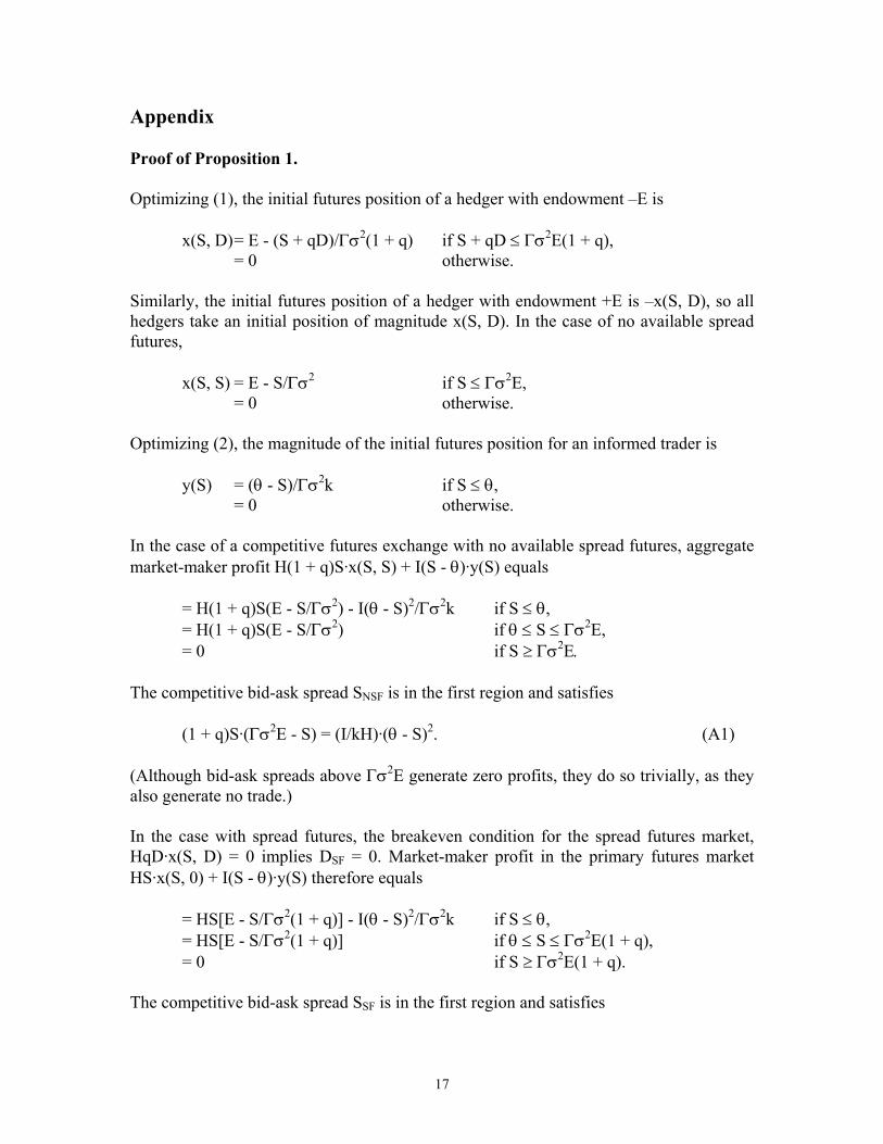
Appendix Proof of Proposition 1. Optimizing (1), the initial futures position of a hedger with endowment –E is x(S, D) = E - (S + qD)/Γσ2(1 + q) if S + qD ≤ Γσ2E(1 + q), = 0 otherwise. Similarly, the initial futures position of a hedger with endowment +E is –x(S, D), so all hedgers take an initial position of magnitude x(S, D). In the case of no available spread futures, x(S, S) = E - S/Γσ2 if S ≤ Γσ2E, = 0 otherwise. Optimizing (2), the magnitude of the initial futures position for an informed trader is y(S) = (θ - S)/Γσ2k if S ≤ θ,
= 0 otherwise. In the case of a competitive futures exchange with no available spread futures, aggregate market-maker profit H(1 + q)S·x(S, S) + I(S - θ)·y(S) equals = H(1 + q)S(E - S/Γσ2) - I(θ - S)2/Γσ2k if S ≤ θ, = H(1 + q)S(E - S/Γσ2) if θ ≤ S ≤ Γσ2E, = 0 if S ≥ Γσ2E. The competitive bid-ask spread SNSF is in the first region and satisfies (1 + q)S·(Γσ2E - S) = (I/kH)·(θ - S)2. (A1) (Although bid-ask spreads above Γσ2E generate zero profits, they do so trivially, as they also generate no trade.) In the case with spread futures, the breakeven condition for the spread futures market, HqD·x(S, D) = 0 implies DSF = 0. Market-maker profit in the primary futures market HS·x(S, 0) + I(S - θ)·y(S) therefore equals = HS[E - S/Γσ2(1 + q)] - I(θ - S)2/Γσ2k if S ≤ θ, = HS[E - S/Γσ2(1 + q)] if θ ≤ S ≤ Γσ2E(1 + q), = 0 if S ≥ Γσ2E(1 + q). The competitive bid-ask spread SSF is in the first region and satisfies
17
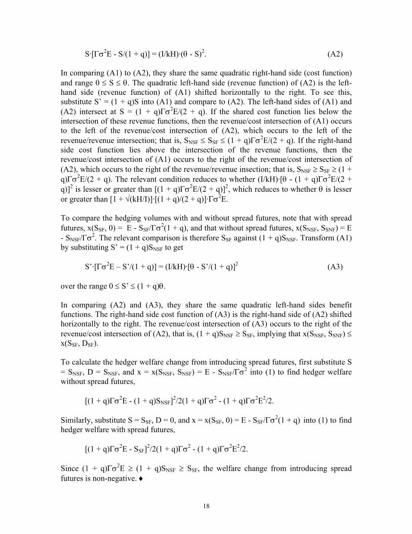
S·[Γσ2E - S/(1 + q)] = (I/kH)·(θ - S)2. (A2) In comparing (A1) to (A2), they share the same quadratic right-hand side (cost function) and range 0 ≤ S ≤ θ. The quadratic left-hand side (revenue function) of (A2) is the left-hand side (revenue function) of (A1) shifted horizontally to the right. To see this, substitute S’ = (1 + q)S into (A1) and compare to (A2). The left-hand sides of (A1) and (A2) intersect at S = (1 + q)Γσ2E/(2 + q). If the shared cost function lies below the intersection of these revenue functions, then the revenue/cost intersection of (A1) occurs to the left of the revenue/cost intersection of (A2), which occurs to the left of the revenue/revenue intersection; that is, SNSF ≤ SSF ≤ (1 + q)Γσ2E/(2 + q). If the right-hand side cost function lies above the intersection of the revenue functions, then the revenue/cost intersection of (A1) occurs to the right of the revenue/cost intersection of (A2), which occurs to the right of the revenue/revenue insection; that is, SNSF ≥ SSF ≥ (1 + q)Γσ2E/(2 + q). The relevant condition reduces to whether (I/kH)·[θ - (1 + q)Γσ2E/(2 + q)]2 is lesser or greater than [(1 + q)Γσ2E/(2 + q)]2, which reduces to whether θ is lesser or greater than [1 + √(kH/I)]·[(1 + q)/(2 + q)]·Γσ2E. To compare the hedging volumes with and without spread futures, note that with spread futures, x(SSF, 0) = E - SSF/Γσ2(1 + q), and that without spread futures, x(SNSF, SSNF) = E - SNSF/Γσ2. The relevant comparison is therefore SSF against (1 + q)SNSF. Transform (A1) by substituting S’ = (1 + q)SNSF to get S’·[Γσ2E – S’/(1 + q)] = (I/kH)·[θ - S’/(1 + q)]2 (A3) over the range 0 ≤ S’ ≤ (1 + q)θ. In comparing (A2) and (A3), they share the same quadratic left-hand sides benefit functions. The right-hand side cost function of (A3) is the right-hand side of (A2) shifted horizontally to the right. The revenue/cost intersection of (A3) occurs to the right of the revenue/cost intersection of (A2), that is, (1 + q)SNSF ≥ SSF, implying that x(SNSF, SSNF) ≤ x(SSF, DSF). To calculate the hedger welfare change from introducing spread futures, first substitute S = SNSF, D = SNSF, and x = x(SNSF, SNSF) = E - SNSF/Γσ2 into (1) to find hedger welfare without spread futures, [(1 + q)Γσ2E - (1 + q)SNSF]2/2(1 + q)Γσ2 - (1 + q)Γσ2E2/2. Similarly, substitute S = SSF, D = 0, and x = x(SSF, 0) = E - SSF/Γσ2(1 + q) into (1) to find hedger welfare with spread futures, [(1 + q)Γσ2E - SSF]2/2(1 + q)Γσ2 - (1 + q)Γσ2E2/2. Since (1 + q)Γσ2E ≥ (1 + q)SNSF ≥ SSF, the welfare change from introducing spread futures is non-negative. ♦
18
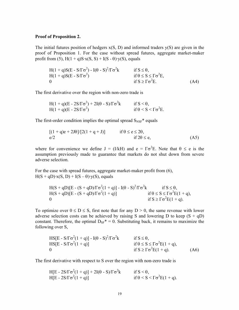
Proof of Proposition 2. The initial futures position of hedgers x(S, D) and informed traders y(S) are given in the proof of Proposition 1. For the case without spread futures, aggregate market-maker profit from (5), H(1 + q)S·x(S, S) + I(S - θ)·y(S), equals H(1 + q)S(E - S/Γσ2) - I(θ - S)2/Γσ2k if S ≤ θ, H(1 + q)S(E - S/Γσ2) if θ ≤ S ≤ Γσ2E, 0 if S ≥ Γσ2E. (A4) The first derivative over the region with non-zero trade is H(1 + q)(E - 2S/Γσ2) + 2I(θ - S)/Γσ2k if S < θ, H(1 + q)(E - 2S/Γσ2) if θ < S < Γσ2E. The first-order condition implies the optimal spread SNSF* equals [(1 + q)e + 2Jθ]/[2(1 + q + J)] if θ ≤ e ≤ 2θ, e/2 if 2θ ≤ e, (A5) where for convenience we define J = (I/kH) and e = Γσ2E. Note that θ ≤ e is the assumption previously made to guarantee that markets do not shut down from severe adverse selection. For the case with spread futures, aggregate market-maker profit from (6), H(S + qD)·x(S, D) + I(S – θ)·y(S), equals H(S + qD)[E - (S + qD)/Γσ2(1 + q)] - I(θ - S)2/Γσ2k if S ≤ θ, H(S + qD)[E - (S + qD)/Γσ2(1 + q)] if θ ≤ S ≤ Γσ2E(1 + q), 0 if S ≥ Γσ2E(1 + q). To optimize over 0 ≤ D ≤ S, first note that for any D > 0, the same revenue with lower adverse selection costs can be achieved by raising S and lowering D to keep (S + qD) constant. Therefore, the optimal DSF* = 0. Substituting back, it remains to maximize the following over S, HS[E - S/Γσ2(1 + q)] - I(θ - S)2/Γσ2k if S ≤ θ, HS[E - S/Γσ2(1 + q)] if θ ≤ S ≤ Γσ2E(1 + q), 0 if S ≥ Γσ2E(1 + q). (A6) The first derivative with respect to S over the region with non-zero trade is H[E - 2S/Γσ2(1 + q)] + 2I(θ - S)/Γσ2k if S < θ, H[E - 2S/Γσ2(1 + q)] if θ < S < Γσ2E(1 + q).
19
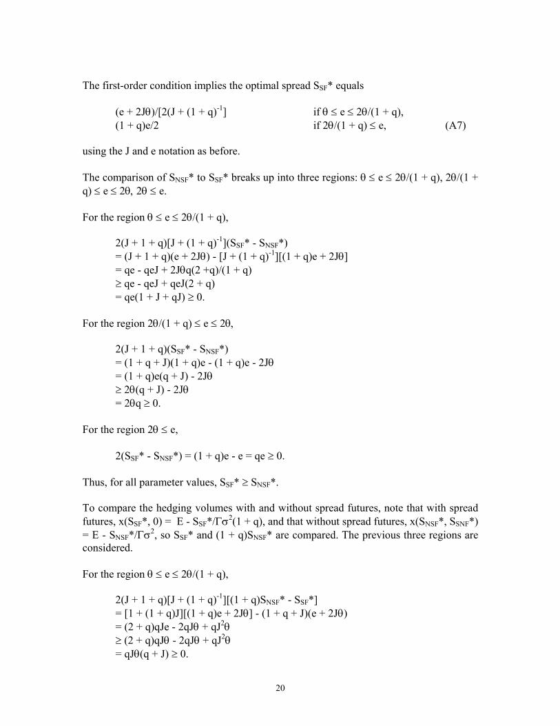
The first-order condition implies the optimal spread SSF* equals (e + 2Jθ)/[2(J + (1 + q)-1] if θ ≤ e ≤ 2θ/(1 + q), (1 + q)e/2 if 2θ/(1 + q) ≤ e, (A7) using the J and e notation as before. The comparison of SNSF* to SSF* breaks up into three regions: θ ≤ e ≤ 2θ/(1 + q), 2θ/(1 + q) ≤ e ≤ 2θ, 2θ ≤ e. For the region θ ≤ e ≤ 2θ/(1 + q), 2(J + 1 + q)[J + (1 + q)-1](SSF* - SNSF*) = (J + 1 + q)(e + 2Jθ) - [J + (1 + q)-1][(1 + q)e + 2Jθ] = qe - qeJ + 2Jθq(2 +q)/(1 + q) ≥ qe - qeJ + qeJ(2 + q) = qe(1 + J + qJ) ≥ 0. For the region 2θ/(1 + q) ≤ e ≤ 2θ, 2(J + 1 + q)(SSF* - SNSF*) = (1 + q + J)(1 + q)e - (1 + q)e - 2Jθ = (1 + q)e(q + J) - 2Jθ ≥ 2θ(q + J) - 2Jθ = 2θq ≥ 0. For the region 2θ ≤ e, 2(SSF* - SNSF*) = (1 + q)e - e = qe ≥ 0. Thus, for all parameter values, SSF* ≥ SNSF*. To compare the hedging volumes with and without spread futures, note that with spread futures, x(SSF*, 0) = E - SSF*/Γσ2(1 + q), and that without spread futures, x(SNSF*, SSNF*) = E - SNSF*/Γσ2, so SSF* and (1 + q)SNSF* are compared. The previous three regions are considered. For the region θ ≤ e ≤ 2θ/(1 + q), 2(J + 1 + q)[J + (1 + q)-1][(1 + q)SNSF* - SSF*] = [1 + (1 + q)J][(1 + q)e + 2Jθ] - (1 + q + J)(e + 2Jθ) = (2 + q)qJe - 2qJθ + qJ2θ ≥ (2 + q)qJθ - 2qJθ + qJ2θ = qJθ(q + J) ≥ 0.
20
For the region 2θ/(1 + q) ≤ e ≤ 2θ, 2(J + 1 + q)[(1 + q)SNSF* - SSF*] = (1 + q)[(1 + q)e + 2Jθ] - (1 + q)e(1 + q + J) = 2(1 + q)Jθ - (1 + q)eJ ≥ (1 + q)Je - (1 + q)eJ = 0. For the region 2θ ≤ e, 2[(1 + q)SNSF* - SSF*] = (1 + q)e - (1 + q)e = 0. For all parameter values, (1 + q)SNSF* ≥ SSF*, implying x(SNSF*, SSNF*) ≤ x(SSF*, DSF*). Calculating the change in hedger welfare from introducing spread futures is similar to the calculation in Proposition 1. Since (1 + q)Γσ2E ≥ (1 + q)SNSF* ≥ SSF*, the welfare change from introducing spread futures is non-negative. ♦ Proof of Proposition 3. The aggregate market-maker profit πNSF* in the case of the monopolistic exchange, without spread futures, can be found by substituting (A5) into (A4). Thus, πNSF* equals (H/Γσ2)( -Jθ2 + [(1 + q)e + 2Jθ]2/4(1 + q + J) ) if θ ≤ e ≤ 2θ, (H/Γσ2)(1 + q)e2/4 if 2θ ≤ e. The aggregate market-maker profit πSF* in the case of the monopolistic exchange, with spread futures, can be found by substituting (A7) into (A6). Thus, πSF* equals (H/Γσ2)( -Jθ2 + (e + 2Jθ)2/4[J + (1 + q)-1] if θ ≤ e ≤ 2θ/(1 + q), (H/Γσ2)(1 + q)e2/4 if 2θ/(1 + q) ≤ e. The difference ∆π* = πSF* - πNSF* gives the increase in market-maker profit from introducing spread futures. Thus, (Γσ2/H) · ∆π* equals (e + 2Jθ)2/4[J + (1 + q)-1] - [(1 + q)e + 2Jθ]2/4(1 + q + J) = qJ[4θe(1 - J) - (2 + q)e2 + 4Jθ2(2 + q)/(1 + q)]/4(1 + q + J)[J + (1 + q)-1] if θ ≤ e ≤ 2θ/(1 + q), (1 + q)e2/4 + Jθ2 - [(1 + q)e + 2Jθ]2/4(1 + q + J) = (1 + q)J(2θ - e)2/4(1 + q + J) if 2θ/(1 + q) ≤ e ≤ 2θ, 0 if 2θ ≤ e. (A8)
21
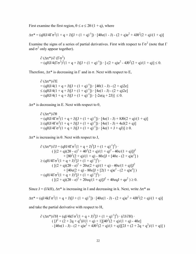
First examine the first region, θ ≤ e ≤ 2θ/(1 + q), where ∆π* = (qHJ/4Γσ2(1 + q + J)[J + (1 + q)-1]) · [4θe(1 - J) - (2 + q)e2 + 4Jθ2(2 + q)/(1 + q)] Examine the signs of a series of partial derivatives. First with respect to Γσ2 (note that Γ and σ2 only appear together). ∂ (∆π*)/∂ (Γσ2)
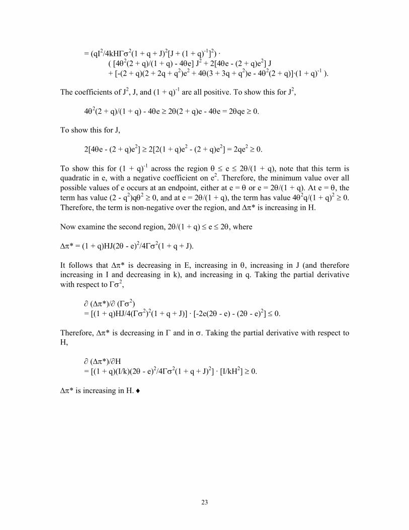
+ [-(2 + q)(2 + 2q + q2)e2 + 4θ(3 + 3q + q2)e - 4θ2(2 + q)]·(1 + q)-1 ). The coefficients of J2, J, and (1 + q)-1 are all positive. To show this for J2, 4θ2(2 + q)/(1 + q) - 4θe ≥ 2θ(2 + q)e - 4θe = 2θqe ≥ 0. To show this for J, 2[4θe - (2 + q)e2] ≥ 2[2(1 + q)e2 - (2 + q)e2] = 2qe2 ≥ 0. To show this for (1 + q)-1 across the region θ ≤ e ≤ 2θ/(1 + q), note that this term is quadratic in e, with a negative coefficient on e2. Therefore, the minimum value over all possible values of e occurs at an endpoint, either at e = θ or e = 2θ/(1 + q). At e = θ, the term has value (2 - q2)qθ2 ≥ 0, and at e = 2θ/(1 + q), the term has value 4θ2q/(1 + q)2 ≥ 0. Therefore, the term is non-negative over the region, and ∆π* is increasing in H. Now examine the second region, 2θ/(1 + q) ≤ e ≤ 2θ, where ∆π* = (1 + q)HJ(2θ - e)2/4Γσ2(1 + q + J). It follows that ∆π* is decreasing in E, increasing in θ, increasing in J (and therefore increasing in I and decreasing in k), and increasing in q. Taking the partial derivative with respect to Γσ2, ∂ (∆π*)/∂ (Γσ2)
= [(1 + q)HJ/4(Γσ2)2(1 + q + J)] · [-2e(2θ - e) - (2θ - e)2] ≤ 0. Therefore, ∆π* is decreasing in Γ and in σ. Taking the partial derivative with respect to H, ∂ (∆π*)/∂H = [(1 + q)(I/k)(2θ - e)2/4Γσ2(1 + q + J)2] · [I/kH2] ≥ 0. ∆π* is increasing in H. ♦
23
References Allen, F., and D. Gale, 1994, Financial Innovation and Risk Sharing, MIT Press, Cambridge, MA. Back, K., 1993, "Asymmetric Information and Options," Review of Financial Studies, 6, 435-472 Bakshi, G., C. Cao, and Z. Chen, 2000, "Do Call Prices and the Underlying Stock Always Move in the Same Direction?," Review of Financial Studies, 13, 549-584. Buraschi, A. and J. Jackwerth, 2001, "The Price of a Smile: Hedging and Spanning in Options Markets," Review of Financial Studies, 14, 495-527. Conrad, J., 1989, "The Price Effect of Option Introduction," Journal of Finance, 44, 487-499. Detemple, J., and P. Jorion, 1990, "Option Listing and Stock Returns: An Empirical Analysis," Journal of Banking and Finance, 14, 781-801. Duffie, D., and R. Rahi, 1995, “Financial Market Innovation and Security Design: An Introduction” Journal of Economic Theory, 65, 1-42. Gray, R. W., 1970, "The Prospects for Trading in Live Hog Futures," in H. H. Bakken (ed.), Futures Trading in Livestock-Origins and Concepts, Chicago Mercantile Exchange, Chicago. Johnston, E., and J. McConnell, 1989, "Requiem for a Market: An Analysis of the Rise and Fall of a Financial Futures Contract," Review of Financial Studies, 2, 1-23. Kyle, A. S., 1984, “Market Structure, Information, Futures Markets, and Price Formation,” in G. G. Storey, A. Schmitz, and A. H. Sarris (eds.), International Agricultural Trade: Advanced Readings in Price Formation, Market Structure and Price Instability, Westview Press, Boulder, CO. Longstaff, F. A., 1995, "Option Pricing and the Martingale Restriction," Review of Financial Studies, 8, 1091-1124. Mayhew, S., 2000, "The Impact of Derivatives on Cash Markets: What Have We Learned?," working paper, University of Georgia. Sandor, R. L., 1973, "Innovation by an Exchange: A Case Study of the Development of the Plywood Futures Contract," Journal of Law and Economics, 16, 119-136. Silber, W. L., 1981, "Innovation, Competition, and New Contract Design in Futures Markets," Journal of Futures Markets, 1, 123-155.
24
Subrahmanyam, A., 1991, "A Theory of Trading in Stock Index Futures," Review of Financial Studies, 4, 17-51. Working, H., 1953, “Futures Trading and Hedging” American Economic Review 43, 314-343.
25
26
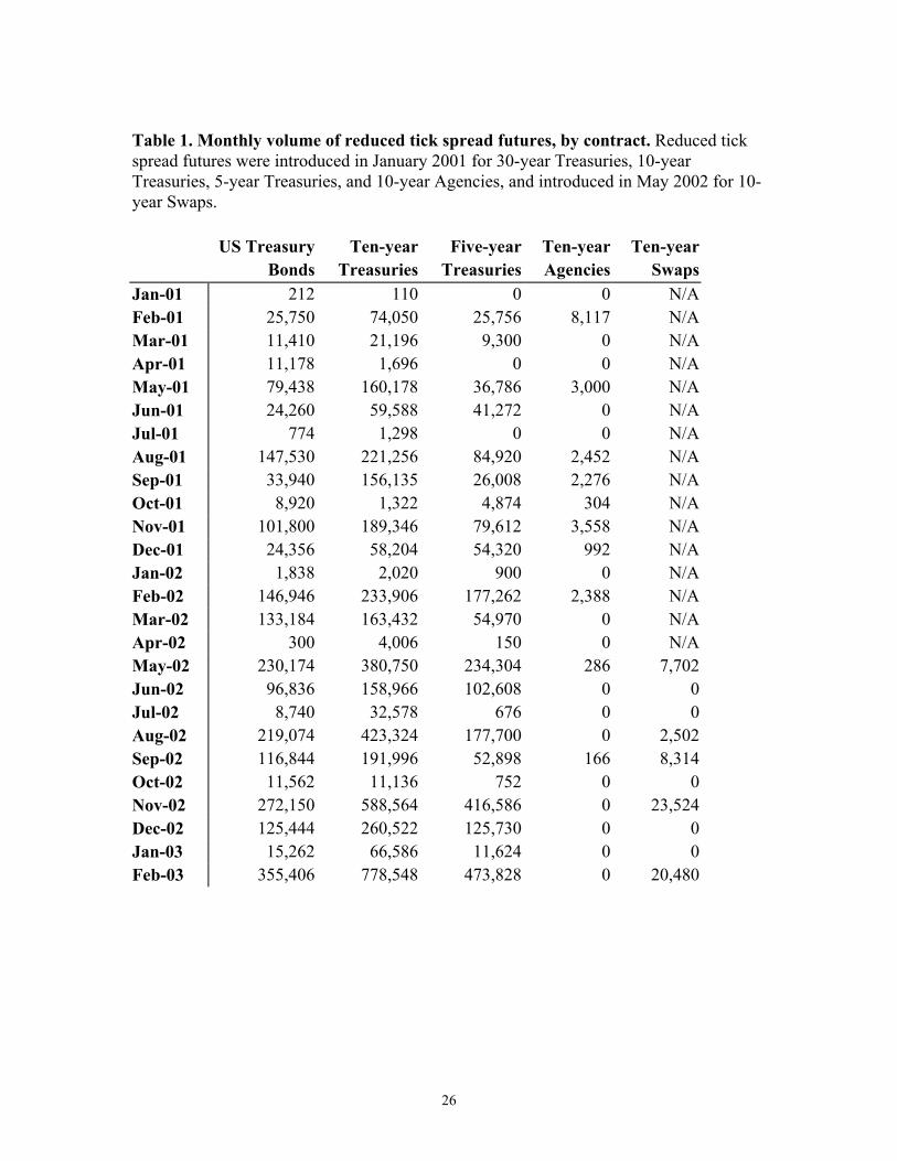
Table 1. Monthly volume of reduced tick spread futures, by contract. Reduced tick spread futures were introduced in January 2001 for 30-year Treasuries, 10-year Treasuries, 5-year Treasuries, and 10-year Agencies, and introduced in May 2002 for 10-year Swaps.