Why Did So Many Subprime Borrowers Default During the Crisis:

Loose Credit or Plummeting Prices?

⇤

Christopher Palmer

†

University of California at Berkeley

September 2015

Abstract

The surge in subprime mortgage defaults during the Great Recession triggered tril-lions of dollars of losses in the financial sector and accounted for more than 50% offoreclosures at the height of the crisis. In particular, subprime mortgages originatedin 2006–2007 were three times more likely to default within three years than mortgagesoriginated in 2003–2004. In the ensuing years of debate, many have argued that this pat-tern across cohorts represents a deterioration in lending standards over time. I confirmthis important channel empirically and quantify the relative importance of an alterna-tive hypothesis: later cohorts defaulted at higher rates in large part because house pricedeclines left them more likely to have negative equity. Using comprehensive loan-leveldata that includes much of the recovery period, I find that changing borrower and loancharacteristics can explain up to 40% of the difference in cohort default rates, with theremaining heterogeneity across cohorts caused by local house-price declines. To accountfor the endogeneity of prices—especially that price declines themselves could have beencaused by subprime lending—I instrument for house price changes with long-run regionalvariation in house-price cyclicality. Control-function results confirm that price declinesunrelated to the credit expansion causally explain the majority of the disparity in co-hort performance. Counterfactual simulations show that if 2006 borrowers had facedthe price paths that the average 2003 borrower did, their annual default rate would havedropped from 12% to 5.6%.

Keywords: Mortgage Finance, Foreclosure Crisis, Subprime Lending, Negative Eq-uity, Hazard Model Control Function

JEL Classification: G01, G21, R31, R38

⇤I thank my advisors, David Autor, Jerry Hausman, Parag Pathak, and Bill Wheaton, for their feedback and en-couragement; discussants Kyle Mangum, Tomek Piskorski, Joe Tracy, Jialan Wang; Haoyang Liu, Sanket Korgaonkar,and Sam Hughes for helpful research assistance; Isaiah Andrews, John Arditi, Matthew Baird, Effi Benmelech, NeilBhutta, John Campbell, David Card, Stan Carmack, Marco Di Maggio, Dan Fetter, Chris Foote, Chris Gillespie,Wills Hickman, Harrison Hong, Erik Hurst, Dwight Jaffee, Amir Kermani, Pat Kline, Lauren Lambie-Hanson, BradLarsen, Fernando Ferreira, Eric Lewis, Andrew Lo, Taylor Nadauld, Whitney Newey, Brian Palmer, Bryan Perry, JimPoterba, Brendan Price, Shane Sherlund, Todd Sinai, Dan Sullivan, Glenn Sueyoshi, Annette Vissing-Jørgensen, ChrisWalters, Nils Wernerfelt, Paul Willen, Heidi Williams, Tyler Williams, and Luigi Zingales for helpful conversationsand feedback; seminar participants at the 2015 AEA meetings, Berkeley, BYU, CFPB, Compass Lexecon, Duke-Fuqua, FDIC, Fed Board, HBS, LBS, LSE, MIT, NBER SI, NEC/CEA, Northwestern-Kellogg, NY Fed, PhiladelphiaFed, Stanford SITE, SF Fed, UCL, the 2014 UEA meetings, Utah State, Wharton, and Yale SOM; and participantsat many MIT and Haas workshops. The loan-level data was provided by CoreLogic. First version: November 2013.

†Professor of Real Estate, Haas School of Business, University of California at Berkeley; cjpalmer@berkeley.edu

1 Introduction

Subprime residential mortgage loans were ground zero in the Great Recession, triggering trillions of

dollars of losses in the financial sector (including precipitating the demise of Bear Sterns and Lehman

Brothers) and comprising over 50% of all 2006–2008 foreclosures despite the fact that only 13% of

existing residential mortgages were subprime at the time.1 The subprime default rate—the number

of new subprime foreclosure starts as a fraction of outstanding subprime mortgages—tripled from

under 6% in 2005 to 17% in 2009. Even AAA subprime residential mortgage-backed securities—

widely held by institutional investors and an important source of repo collateral at the time—had

lost 60% of their value by 2009. By 2013, more than one in five subprime loans originated since

1995 had defaulted.

Why did the performance of subprime loans decline so sharply? A focal point of the discussion

has been the stylized fact that subprime mortgages originated in 2005–2007 performed significantly

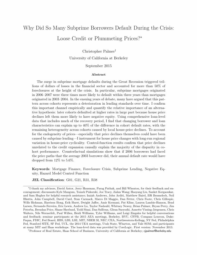
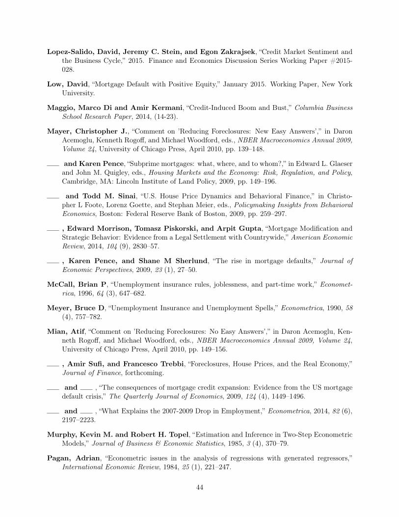
worse than subprime mortgages originated in 2003–2004.2 This is visible in the top panel of Figure

1, which uses data from subprime private-label mortgage-backed securities to show this pattern for

2003–2007 borrower cohorts.3 Each line shows the cumulative fraction of borrowers in the indicated

cohort that defaulted within a given number of months from origination.4 The pronounced pattern

is that the speed and frequency of default are higher for later cohorts—within any number of

months since origination, each cohort has defaulted at a higher rate than the one previous to it

(with the exception of the 2007 cohort in later years). For example, within two years of origination,

approximately 20% of subprime mortgages originated in 2006–2007 had defaulted, in contrast with

approximately 5% of 2003-vintage mortgages.

Because a disproportionate share of subprime defaults came from later cohorts, understanding

why these cohorts performed so poorly informs discussion on the causes of the subprime crisis and

is important for designing effective policy. In particular, the extent to which the cohort pattern was

1Statistics derived from the Mortgage Bankers Association National Delinquency Survey. For the purposes of thispaper, subprime mortgages are defined as those in private-label mortgage-backed securities marketed as subprime, asin Mayer et al. (2009). For an estimate of the effects of foreclosures on the real economy, see Mian et al. (forthcoming).

2See JEC (2007), Krugman (2007b), Gerardi et al. (2008), Haughwout et al. (2008), Mayer et al. (2009), Demyanykand Van Hemert (2010), Krainer and Laderman (2011), and Bhardwaj and Sengupta (2012 and 2014) for examplesof contrasting earlier and later borrower cohorts.

3This data will be discussed at length in Section 3. The analysis stops with the 2007 cohort because by 2008 thesubprime market was virtually nonexistent—the number of subprime loans originated in 2008 in the securitizationdata fell by 99% from the number of 2007 originations.

4Following Sherlund (2008) and Mayer et al. (2009), I measure the point in time when a mortgage has defaultedas the first time that its delinquency status is marked as in the foreclosure process or real-estate owned provided itultimately terminated without being paid off in full.

1

caused by selection (changes in the composition of cohorts) or circumstances (the stronger incidence

of price declines on recent borrowers) is an important input into both ex-ante and ex-post policies

(e.g. macroprudential credit market regulation and loan modification programs, respectively). On

the selection side, a popular explanation for the increase in cohort default rates over time is that

loosening lending standards led to a change in the composition of subprime borrowers, potentially

on both observable (e.g. JEC, 2007 and COP, 2009) and unobservable dimensions (Keys et al., 2008

and Rajan et al., 2015). Related, others (e.g. Krugman, 2007a) blame an increase in the popularity

of non-traditional mortgage products, some arguing that if distressed borrowers had less exotic

mortgage products, their distress wouldn’t have happened in the first place (e.g. Bair, 2007). These

explanations are both consistent with the observed heterogeneity in cohort-level outcomes seen in

Figure 1, which could be generated by a decrease in borrower creditworthiness or an increase in

the riskiness of originated mortgage characteristics, and motivate policies that place restrictions on

allowable mortgage contracts.

Another likely channel is that price declines in the housing market—national prices declined

by 37% between 2005–2009—differentially affected later cohorts, who had accumulated less equity

when property values began to plummet (see, for example, Feldstein, 2011). There are at least

three reasons why falling property values could cause defaults: negative equity, price expectations,

and housing-market liquidity. Having negative equity or being underwater—owing more on an asset

than its current market value—is an important friction in credit markets. Borrowers who can no

longer afford their mortgage payments can sell their homes or use their equity to refinance into

a mortgage with a lower monthly payment if they have sufficient equity. Such alternatives are

generally unavailable for distressed underwater homeowners—lenders are most often unwilling to

refinance underwater mortgages or allow short sales (where the purchase price is insufficient to

cover liens against the property). Second, beliefs about future price changes may also play a role in

default decisions. For a given level of negative equity, underwater homeowners extrapolating based

on strong price declines may default strategically to discharge their mortgage debt if they deem

the option value of holding onto their property to be low, with potential short-sale buyers similarly

spooked by extrapolative expectations.5 Third, falling prices can have affect default independent of

the frictions associated with negative equity. Lazear (2012) provides an explanation for why volume

and price move together in housing markets, meaning that illiquidity will be particularly acute

5Bhutta et al. (2010) find that half of defaults are strategic (in the sense that they are not driven by incomeshocks) among borrowers whose property value is less than half of the outstanding principal balance. Other evidencesuggests that underwater borrowers become delinquent in search of a mortgage modification (Mayer et al., 2014).

2

when demand is low. Low (2015) documents that the time-varying illiquidity of owner-occupied

housing market can lead to positive-equity defaults. Extrapolative beliefs may spook potential

buyers, further depressing prices and exacerbating illiquidity (Glaeser and Nathanson, 2015 and

Barberis et al., 2015).

In this paper, I investigate the relative importance of each of these potential causes of declin-

ing cohort outcomes—price declines and compositional changes in borrowers and mortgages—to

understand what caused the increase in subprime defaults during the Great Recession. The coun-

terfactual question I ask is whether this last-in, first-out pattern of cohort default rates would have

persisted if the better-performing early cohorts had instead faced the market conditions experienced

by the later cohorts. If 2003 borrowers, with their less-exotic mortgages and less-risky attributes,

would have mimicked the performance of 2006 borrowers if they hadn’t experienced mid-2000s home

price appreciation, then this limits the scope of mortgage-lending regulation to produce a resilient

population of borrowers who can withstand significant home price shocks.

To answer these questions, I estimate semiparametric hazard models of default using a panel

of subprime loans that combines rich borrower and loan characteristics with monthly updates on

loan balances, property values, delinquency statuses, and local price changes. I find that differential

exposure to price declines explains at least 60% of the heterogeneity in cohort default rates. I

also estimate that the changing product characteristics of subprime mortgages (and correlated

changes in unobservable borrower quality) play an important role, accounting for 30% of the rise

in defaults across cohorts. Conditioning on price changes and loan and borrower characteristics

explains almost the entire deterioration in cohort-level default rates, suggesting that the model

captures the cohort pattern quite well. Returning to the counterfactual question posed above, my

counterfactual simulations imply that if 2003 borrowers had faced the prices that the average 2006

borrower did (i.e. at the same number of months since origination), 2003 borrowers would have

defaulted twice as frequently, at an annual default rate of 8.5% instead of 4.2%. These results

call into question the practice of inferring the success or failure of a lending-standards regime from

cohort-level outcomes. Are waves of default always an indication of inadequate lending standards?

No, and just as overattribution of the cohort pattern to lending practices during the crisis may have

led to an overreliance on tighter lending as a policy response, using the low rate of foreclosures

for cohorts originated since the crisis as evidence that stronger mortgage regulation was a success

overlooks the likely role of the house price recovery in explaining much of that improvement.

Employing prices as an explanatory variable is risky business from an identification standpoint.

3

As home prices are an equilibrium outcome that depend on other factors related to default risk, the

potential for both price changes and defaults to be caused by a third factor may lead to estimating

a spurious effect of price changes and defaults. Indeed, some commentators have argued that price

declines were merely an outcome of the same weak lending standards that caused the foreclosure

crisis, in which case tighter lending standards would be a panacea. In other words, some of the

sources of price shocks may also have direct effects on the (static) unobserved quality of borrowers

or the (dynamic) subsequent economic environment faced by borrowers and hence on defaults.

A prominent hypothesis is that subprime penetration itself may subsequently have caused price

declines and defaults, as suggested by Mayer and Sinai (2007), Mian and Sufi (2009), Pavlov and

Wachter (2011), and Di Maggio and Kermani (2014).6 Initially, a credit expansion could amplify

the price cycle, initially increasing prices from the positive demand shock as the pool of potential

buyers grows. However, the decrease in average borrower quality from the credit expansion could

eventually lead to an increase in defaults, accelerating price declines. Thus, even though individual

borrowers are price takers in the housing market, a cohort’s average unobserved quality may be

correlated with the magnitude of the price declines its borrowers face, resulting in biased estimates

of the causal effect of prices on default risk. Likewise, a simple reverse causality story—defaults

cause price declines—could bias results up or down depending on the relative magnitude of the

forward and reverse channels. This endogeneity challenge complicates identifying the sources of

outcome differences across cohorts.

To isolate the portion of cohort default rates causally driven by price changes, I exploit plausibly

exogenous long-run variation in metropolitan-area home-price cyclicality. As observed by Sinai

(2012), there is persistence in the amplitude of home-price cycles—cities with strong price cycles

in the 1980s were more likely to have strong cycles in the 2000s. I use this historical variation

in home-price volatility to construct counterfactual price indices, which, crucially, are unrelated to

housing market shocks unique to the 2000s price cycle because price volatility in the 1980s occurred

well before the widespread adoption of subprime mortgages, as I demonstrate below. Indeed, I show

below that my instrument does not predict differential subprime expansion. I also verify that my

results are robust to controlling for local unemployment rates.

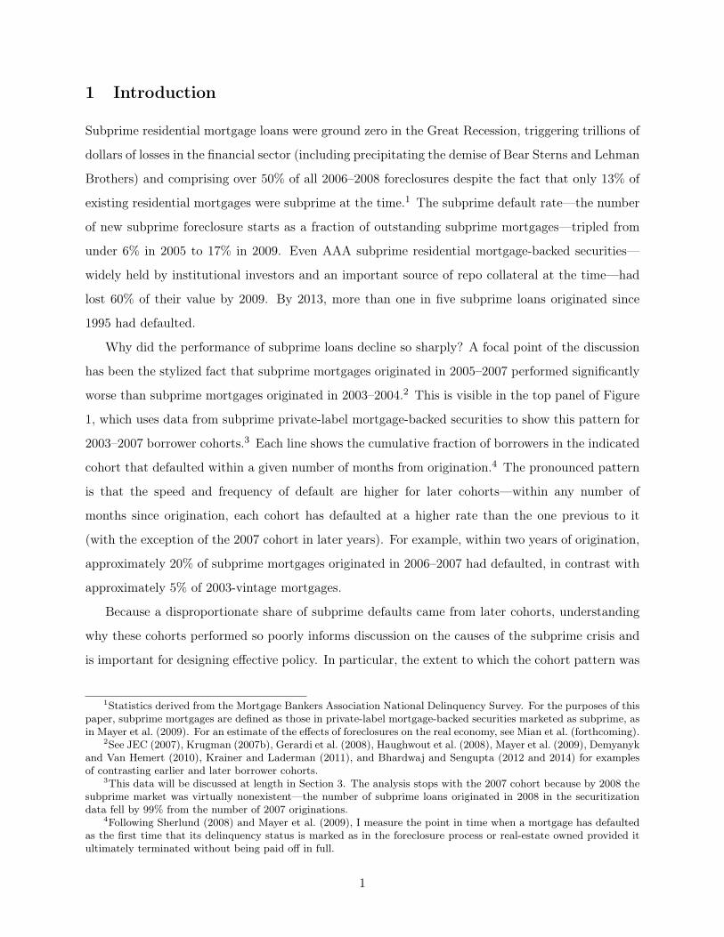
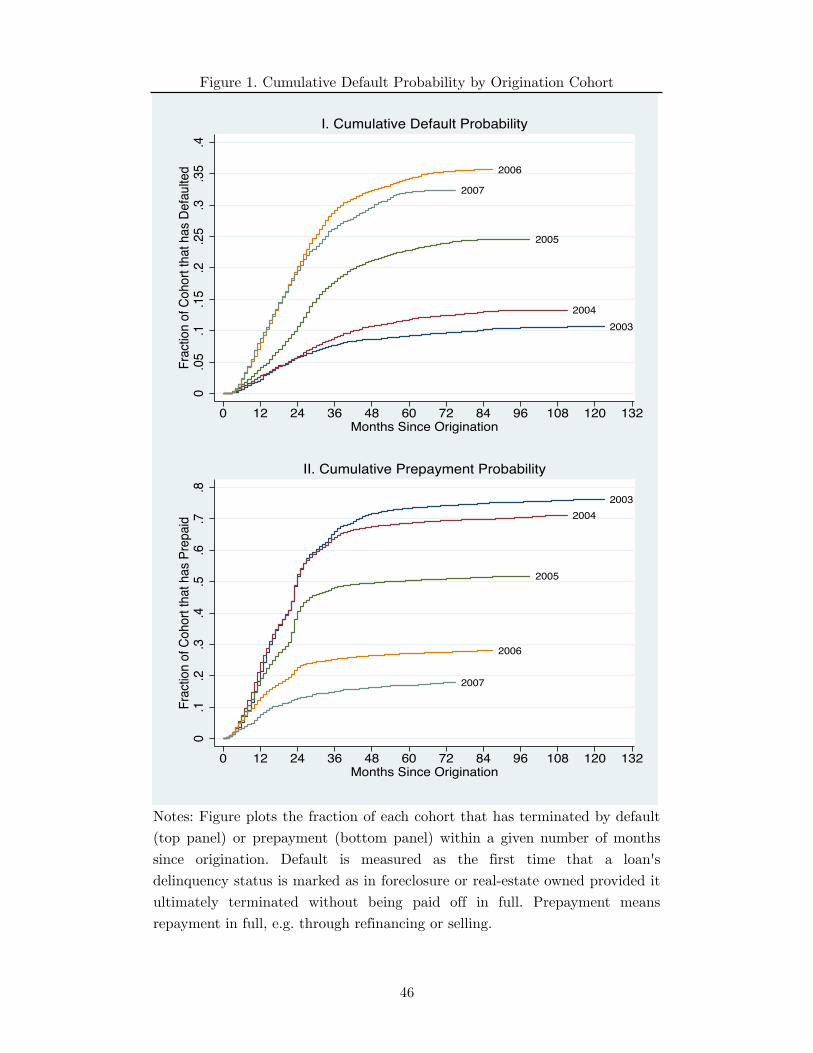
Figure 2 illustrates the differential effect that declining home prices had on origination cohorts

by plotting the median mark-to-market combined loan-to-value ratio (CLTV) of each cohort of bor-

6A parallel literature uses international aggregate data to show the simultaneity of asset-price and credit bubbles,e.g. Jorda et al. (2011).

4

rowers over time.7 The beginning of each line shows the median CLTV at origination for mortgages

taken out in January of that cohort’s birth year. Thereafter, each line shows the median CLTV of all

existing mortgages in the indicated origination cohort.8 Each cohort’s median CLTV began rising in

2007 as prices declined nationwide. However, there are two main differences between early and late

cohorts. First, origination CLTVs increased over time—the median 2007 CLTV was 10 percentage

points higher than the median 2003 CLTV, lending credence to the argument that underwriting

standards deteriorated. Second, earlier cohorts’ median CLTVs declined from origination until 2007

as prices rose (increasing the CLTV denominator) and as borrowers made their mortgage payments,

reducing their indebtedness (the CLTV numerator), with the former effect dominating because of

the low amount of principal paid off early in the mortgage amortization schedule. In contrast,

later cohorts had not accumulated any appreciation or paid down any principal as prices fell almost

immediately after their origination dates. By early 2008, more than one-half of borrowers in both

the 2006 and 2007 cohorts were underwater, and by early 2009, more than one-half of the 2005

cohort was underwater. Using variation in price changes across cities and cohorts and controlling

for CLTV at origination, the empirical specifications below allow me to identify the causal effect of

collateral value shocks on defaults, differentiating between differences in negative equity prevalence

across cohorts explained by high CLTVs at origination (a component of cohort quality) and less

opportunity to accumulate equity before price declines begin.

Suggestive evidence that the prevalence of negative equity affected economic outcomes is the

bottom panel of Figure 1, which shows the cumulative prepayment probability by cohort—the

fraction of each cohort’s mortgages that had been paid off within the given number of months

since origination.9 The pattern across cohorts is exactly reversed from the cohort heterogeneity

in default rates depicted in the top panel—more recent borrowers prepaid their mortgages much

less frequently and at slower rates than borrowers from 2003–2005. Given the evidence that later

cohorts were more likely to be underwater, the contrast between the cohort-level trends in defaults

and prepayments is consistent with the notion that underwater borrowers in distress default and

7The combined loan-to-value ratio (CLTV) of a mortgage is the sum of all outstanding principal balances securedby a given property divided by the value of that property. The data used in Figure 2 estimate market values fromCoreLogic’s Automated Valuation Model, see Section 3 for more details.

8Having a high CLTV at origination (equivalent to having a small down payment) is highly correlated with defaultrisk and is routinely factored into the interest rates charged by lenders.

9Note that in bond markets, prepayment means payment in full. As the issuer of a callable bond, a mortgageborrower has the prerogative to pay back the debt’s principal balance at any time, releasing them of further obligationto the lender. In practice, this is done through refinancing or selling the home and using the proceeds to pay backthe lender.

5

above-water borrowers in distress prepay.10

To my knowledge, this paper is the first to instrument for home prices to address the joint

endogeneity of prices and defaults. There is a broad literature on the determinants of mortgage

default.11 While many researchers have looked at the relationship between home-price appreciation

and defaults, none of them has addressed the endogeneity of home-price changes.12 Using a control-

function approach to account for the endogeneity of covariates in a hazard model setting, I confirm

my main results that prices are endogenous, they are an important determinant of default, and they

account for over half of the cohort pattern in default rates.

A number of studies have examined the proximate causes of the subprime foreclosure crisis

(see Keys et al., 2008, Hubbard and Mayer, 2009, Mian and Sufi, 2009, and Dell’Ariccia et al.,

2012), many of which have the flavor of Minsky (1986) that a period of steady appreciation dulled

underwriting standards and screening vigilance. Corbae and Quintin (2015) provide a theoretical

model demonstrating how a period of relaxed underwriting standards could lead to a mass of

mortgages originated to borrowers who would subsequently be extraordinarily sensitive to price

declines. Several papers have tried to quantify the relative contributions of underwriting standards

and housing market conditions in the increase in the subprime default rate over time (all treating

metropolitan area home price changes as exogenous) and have generally found a residual decrease

in cohort quality. Sherlund (2008) concludes that leverage is the strongest predictor of increasing

default risk and decreasing prepayment risk among subprime loans. Gerardi et al. (2008) use data

through 2007 to ask whether lenders, investors, and rating agencies should have known that price

declines would induce widespread defaults. Kau et al. (2011) find that the secondary mortgage

market was aware of an ongoing decline in subprime borrower quality. Gerardi et al. (2013) look at

the importance of negative equity and employment shocks. Bajari et al. (2008) estimate a dynamic

model of default behavior on subprime mortgage data from 20 metropolitan areas and find evidence

supporting both lending standards and price declines as drivers of default.

Many papers explicitly analyze differences in default or delinquency across cohorts. Haughwout

et al. (2008) and Mayer et al. (2009) demonstrate heterogeneity in the early-default rates of origi-

10Note that this pattern could also be generated by cohort quality if riskier borrowers prepay less frequently,e.g. if they are less likely to take advantage of in-the-money prepayment options or less likely to trade-up to a moreexpensive home.

11For example, Deng et al. (2000), Foote et al. (2008), Pennington-Cross and Ho (2010), and Bhutta et al. (2010).12For example, the common practice of imputing changes in property values using a metropolitan area home price

index, although free from property-specific price shocks, does not address the concern that price changes at themetropolitan-area level are themselves the outcome of demand and supply shocks that are plausibly correlated withunobserved borrower quality.

6

nation cohorts and document that loosening downpayment requirements and declining home prices

are both highly correlated with increases in early defaults. Using data ending in 2008, Demyanyk

and Van Hemert (2011) consider vintage effects in borrower quality and find that that the bulk of

the deterioration in vintage quality was due to unobservables, suggesting that the lending boom

coincided with increasing adverse selection among borrowers. Krainer and Laderman (2011) and

Bhardwaj and Sengupta (2012) find that prepayment rate declines across cohorts are concurrent

with default rate increases.

In summary, existing academic work has focused on whether changes in loan origination charac-

teristics explain changes in default rates or whether prevailing market conditions such as negative

equity were acute in areas where many borrowers are defaulting. In a world where price declines are

themselves caused by lending activity (in other words, given the feedback between asset and credit

markets), these results are somewhat hard to interpret. In contrast to these papers, with the benefit

of an identification strategy and several more years of data on the 2003–2007 subprime borrower

cohorts, I am able to separate the effect of price changes on default rates from the effect of lending

standards on default and explain virtually the entire cohort pattern.13 Intuitively, I compare cohorts

in areas with exogenously different price cycles (and thus differing predicted amounts of negative

equity) to estimate whether they also had different default patterns after adjusting for observable

underwriting characteristics.

The paper proceeds as follows. Section 2 discusses the empirical strategy. I describe the data

and compare the observable characteristics of borrower cohorts in Section 3. Identification concerns

in the context of a hazard model are detailed in Section 4, along with a description of the estimator.

After presenting initial descriptive estimates of the determinants of default that drive the cohort

pattern, Section 5 presents the control-function strategy and my main results, and Section 6 explores

the economic mechanisms through which price declines affect default rates. Using my preferred

empirical specification, I estimate cohort-level default rates under several counterfactual scenarios

in Section 7. In Section 8, I conclude by summarizing my main findings and briefly discussing policy

implications.

13Hertzberg et al. (2015) describe a consumer-loan setting where inference about cohort quality after only oneyear is a misleading indicator of eventual performance differences, pointing to the importance of looking past earlymortgage defaults.

7

2 Empirical Strategy

Many factors determine default risk. Underwriting standards and market conditions, each predictive

of future idiosyncratic income shocks and changes in prepayment opportunities, interact to explain

realized defaults. Loose underwriting standards increase default rates because equally sized negative

income shocks are more likely to prevent borrowers with high debt-to-income ratios from making

mortgage payments and because borrowers with riskier income are more likely to have a negative

shock that prevents them from making their mortgage payments. After a period of sustained price

growth, younger loans are also relatively more sensitive to price declines because they have not

accumulated as much equity and are thus more apt to be underwater and constrained in their

ability to sell or refinance their mortgage. If an equal share of each cohort has an income shock

that prohibits them from paying back their mortgage, cohorts with positive equity will simply sell

their homes or refinance into mortgages with better terms. Later cohorts, on the other hand, have

no such option and will default.

The objective of the hazard models presented below is to examine the relative importance of each

of these factors by comparing loans with differing underwriting characteristics and in areas with

differing price cycles to estimate how much of the heterogeneity in cohort default rates is explain-

able by each factor. Comparing observationally similar loans (i.e. by controlling for underwriting

standards and loan age with a flexible baseline hazard specification) within a geography that were

originated at different times allows me to take advantage of temporal variation in home prices within

a geographic region. Likewise, comparing observationally similar loans taken out at the same time

but in different cities utilizes spatial variation in home prices. To account for the endogeneity of the

home price series of each geographic area, I estimate counterfactual price series by mapping each

area’s 1980–1995 home price volatility onto the most recent price cycle, as discussed in detail in

Section 4 below. This setup allows me to decompose observed cohort heterogeneity into its driving

factors by successively introducing additional controls that explain away the differences in cohort

default rates.

Hazard Model Specification I specify the origination-until-default duration as a propor-

tional hazard model with time-varying covariates. Although the data are grouped into monthly ob-

servations, the proportional-hazards functional form allows estimation of a continuous-time hazard

model using discrete data (Prentice and Gloeckler, 1978 and Allison, 1982). Let the latent time-to-

default random variable be denoted ⌧ , and let the instantaneous probability (i.e. in continuous-time)

8

of borrower i in cohort c and geography g defaulting at month t given that borrower i has not yet

defaulted specified as

lim

⇠!0+

Pr

�⌧ 2 (t� ⇠, t]

��⌧ > t� ⇠�

⇠⌘ �(Xicg(t), t) (1)

= exp(X 0icg(t)�)�0(t) (2)

where �0(·) is the baseline hazard function that depends only on the time since origination t, and

Xicg(t) is a vector of time-varying covariates that in practice will be measured at discrete monthly

intervals. The proportional hazards framework assumes that the conditional default probability

depends on the elapsed duration through a baseline hazard function that is shared by all mortgages

and is scaled up and down by covariates to capture the effects of observable individual heterogeneity.

A convenience of this framework is that the coefficient vector � is readily interpretable as measuring

the effect of the covariates on the log hazard rate.

Combining a nonparametric baseline hazard function with covariates entering through a para-

metric linear index function results in a semiparametric model of default. The specification for the

covariates is

X 0icg(t)� = �c +W 0

B,i✓B +W 0L,i✓L + µ ·�Pricesicg(t) + ↵g (3)

where �c and ↵g are cohort and geographic fixed effects, respectively; WB and WL are vectors of bor-

rower (B) and loan (L) attributes, measured at the time of mortgage origination; and �Pricesicg(t)

is a measure of the change in prices faced by property i at time t.14 Borrower characteristics include

the FICO score (a credit score measuring the quality of the borrower’s credit history), debt-to-

income (DTI) ratio (calculated using all outstanding debt obligations), an indicator variable for

whether the borrower provided full documentation of income during underwriting, and an indicator

variable for whether the property was to be occupied as a primary residence. Attributes of the

mortgage note include the combined loan-to-value ratio at origination (using all open liens on the

property for the numerator and the sale price for the denominator), the mortgage interest rate,

and indicator variables for adjustable-rate mortgages, cash-out refinance mortgages (when the new

mortgage amount exceeds the outstanding principal due on the previous mortgage secured by the

same house), mortgages with an interest-only period (when payments do not pay down any princi-

14A natural concern with including fixed effects ↵g in a nonlinear panel data model like this is the incidentalparameters problem, which arises when the observations per group g is small and the number of groups grows withthe sample size such that no progress is made in reducing the variance of the estimated fixed effects. Unlike a panelwith fixed effects for each individual, the details of this application suggest this is not a significant worry. The numberof observations per geography is already quite large, and as the total number of observations increases, the numberof metropolitan areas in the U.S. remains fixed, leading to consistent estimates of ↵g.

9

pal), balloon mortgages (non-fully amortizing mortgages that require a balloon payment at the end

of the term), and mortgages accompanied by additional so-called piggyback mortgages.

The cohort fixed effects �c are the parameters of interest. As 2003 is the omitted cohort,

the estimated baseline hazard function represents the conditional probability of default for a 2003

mortgage of each given age. The �c parameters scale this up or down depending on how cohort

c mortgages default over their life-cycle, conditional on X and relative to 2003 mortgages of the

same duration. Successively conditioning on geographic fixed effects, borrower characteristics, loan

characteristics, and price changes reveals the extent to which each factor explains the systematic

variation in default risk across cohorts. The estimated �̂c without conditioning on any covariates

are a measure of the average performance of each cohort. Conditioning on prices, the �c are an

estimate of the quality of each cohort, where quality is estimated using an ex-post measure (defaults).

Conditioning on observable loan and borrower characteristics and prices, the �c represents the latent

(i.e. unobserved) quality of each cohort. If cohort-level mortgage performance differences were driven

by borrower unobservables, or if the explanatory power of the observables declined over time, then

this would be captured by the cohort coefficients after controlling for all observables.

3 Data and Descriptive Statistics

In this section I briefly describe the data sources used in my analysis.

CoreLogic LoanPerformance (LP) Data. The main data source underlying this paper

is the CoreLogic LoanPerformance (LP) Asset-Backed Securities database, a loan-level database

providing detailed information on mortgages in private-label mortgage-backed securities including

static borrower characteristics (DTI, FICO, owner-occupant, etc.), static loan characteristics (LTV,

interest rate, purchase mortgage, etc.), and time-varying mortgage attributes updated monthly

such as delinquency status and outstanding balance.15 The LP data record monthly loan-level data

on most private-label securitized mortgage balances, including an estimated 87% coverage of out-

standing subprime securitized balances. Because about 75% of 2001–2007 subprime mortgages were

securitized, this results in over 65% coverage of the subprime mortgage market.16 My estimation

15Using LP data is standard in the economics literature for microdata-based analysis of subprime and near-prime loan performance. See Sherlund (2008), Mayer et al. (2009), Demyanyk and Van Hemert (2011), Krainer andLederman (2011), and Fuster and Willen (2015) for examples. See GAO (2010) for a more complete discussion of theLP database and comparison with other loan-level data sources.

16See Mayer and Pence (2009) for a description of the relative representativeness of subprime data sources. Footeet al. (2009) and Elul (2015) suggest that non-securitized subprime mortgages are less risky than securitized ones.

10

sample is formed from a 1% random sample of first-lien subprime mortgages originated in 2003–2007

in the LP database, resulting in a final dataset of over one million loan ⇥ month observations.17

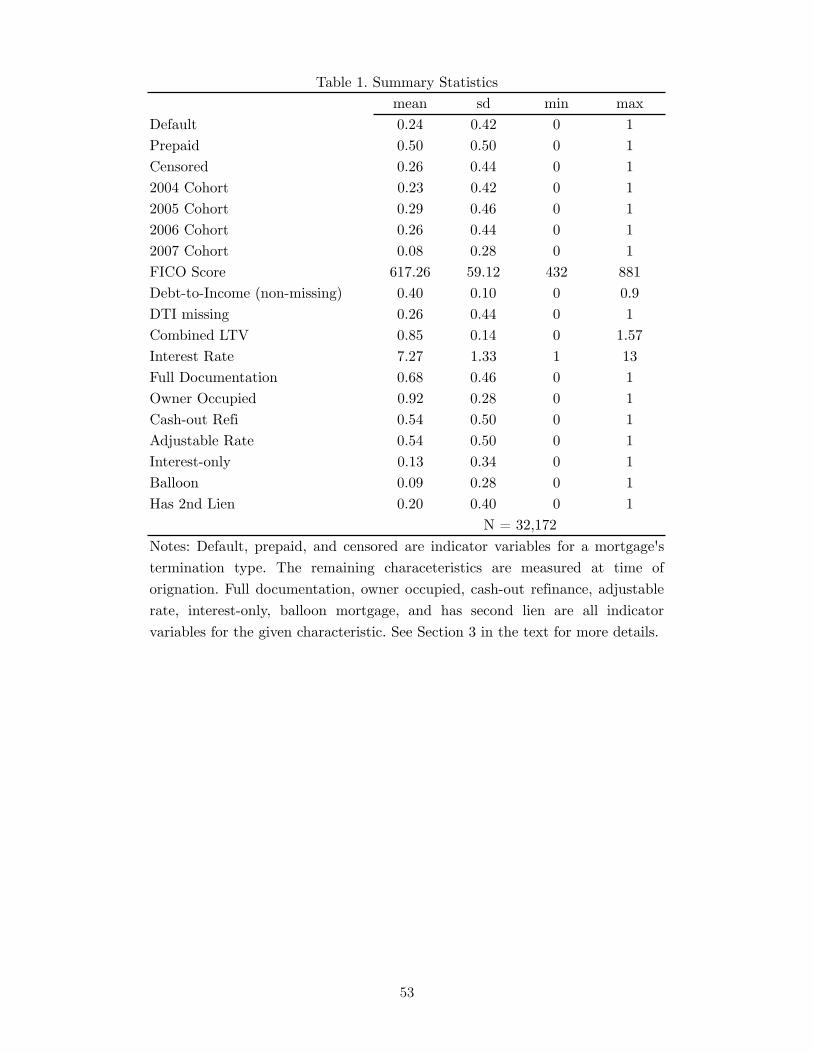
Table 1 reports descriptive statistics for static (at time of origination) loan-level borrower and

mortgage characteristics. On these observable dimensions, it is clear that subprime borrowers

comprised a population with high ex-ante default risk. The average subprime borrower in my data

had a credit score of 617, slightly above the national 25th percentile FICO score and substantially

below the national median score of 720 (Board of Governors of the Federal Reserve System, 2007).

Among borrowers who reported their income on their mortgage application, the average back-end

debt-to-income ratio, which combines monthly debt payments made to service all open property

liens, was almost 40%, well above standard affordable housing thresholds. More than half of the

loans in my estimation sample were for cash-out refinances, where the borrower is obtaining the new

mortgage for an amount higher than the outstanding balance of the prior mortgage. As of April

2013, when my data end, 24% of the mortgages in my sample have defaulted and 50% have been

paid off, leaving 26% of the loans in the data still outstanding.

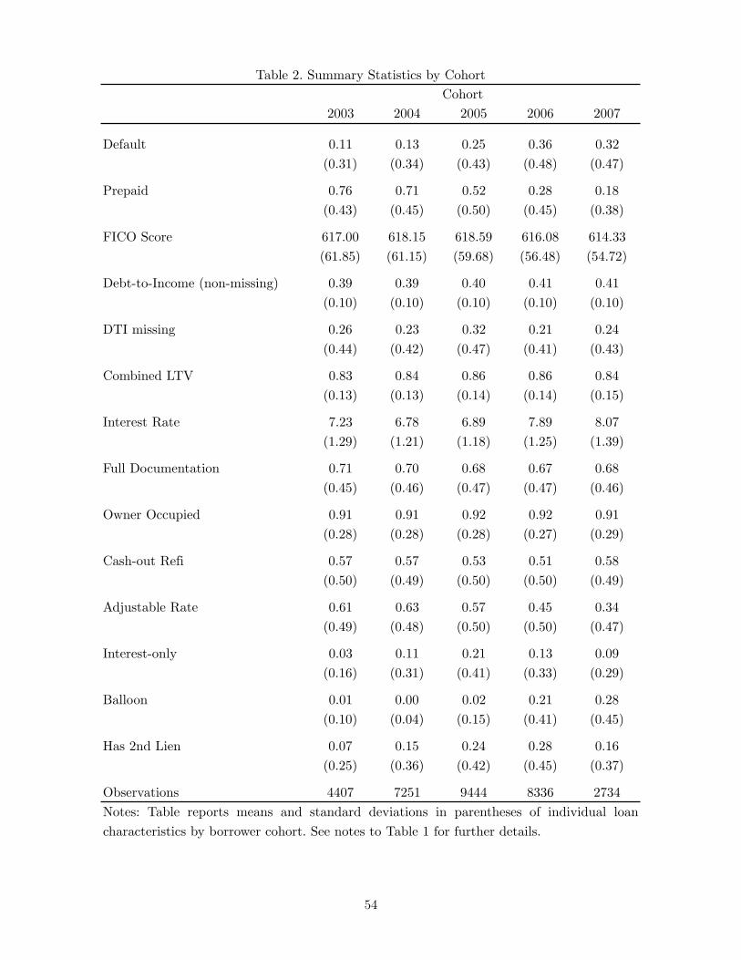
Table 2 presents descriptive statistics by origination cohort. The distribution of many borrower

characteristics is stable across cohorts. Average FICO scores, DTI ratios, combined loan-to-value

ratios (measured using all concurrent mortgages and the sale price of the home, both at the time of

origination), documentation status, and the fraction of loans that were owner-occupied or were taken

out as part of a cash-out refinance are roughly constant across cohorts.18 While there is substantial

evidence that, pooling prime, near-prime, and subprime mortgages, borrower characteristics were

deteriorating across cohorts (see JEC, 2007), the lack of a noticeable decrease in borrower observables

in my data is consistent with observations from Gerardi et al. (2008) and Demyanyk and Van

Hemert (2011) who argue that the declines within the population of subprime borrowers were too

small to account for the heterogeneity in performance across cohorts.19 Among mortgage product

17There is no standardized definition of a subprime mortgage, although the term always means a loan deemedto have elevated default risk. Popular classification methods include mortgages originated to borrowers with acredit score below certain thresholds, mortgages with an interest rate that exceeds the comparable Treasury rateby three percentage points, certain mortgage product types, mortgages made by lenders who self-identify as makingpredominantly subprime mortgages, and mortgages serviced by firms that specialize in servicing subprime mortgages.For my purposes a subprime loan is one that is in a mortgage-backed security that was marketed at issuance assubprime, as in Mayer et al. (2009). I additionally drop mortgages originated for less than $10,000, mortgages whosefirst payment date is before the origination date or 90 days after the origination date, and non-standard propertytypes such as manufactured housing following Sherlund (2008).

18Note that the at-origination CLTVs reported here use the sale price of the home for its value, whereas thecontemporaneous (mark-to-market) CLTVs in Figure 2 use estimated market values. If the divergence between thesetwo measures over time is an important predictor of default, it will affect the magnitude of the estimated cohort maineffects, which capture all unobserved factors changing across cohorts.

19Still, the nationwide decline in underwriting standards was driven in part by the subprime expansion: Even

11

characteristics, however, there are important differences across cohorts, including a marked increase

in prevalence of interest-only loans, mortgages with balloon payments, and mortgages accompanied

by additional liens on the property. This finding of relatively stable borrower observables and large

changes in certain mortgage characteristics is consistent with the findings of Rajan et al. (2015) and

Mayer et al. (2009). Still, the distinction between borrower and product characteristics is artificial—

certainly changing product attributes changes the composition of borrowers selecting into subprime

mortgages with the specified features.

Specifications which directly examine the effects of negative equity make use of a novel feature

of the LP dataset: contemporaneous combined loan-to-value ratios (CLTVs), which are a measure

of the total amount of debt secured against a property relative to its market value. To calculate

the CLTV numerator, CoreLogic uses public records filings on additional liens on the property to

estimate the total debt secured against the property at origination. For the denominator, CoreL-

ogic has an automated valuation model (popular in the mortgage lending industry) that uses the

characteristics of a property combined with recent sales of comparable properties in the area and

monthly home price indices to impute a value for each property in each month.

CoreLogic Home Price Index. For regional measures of home prices, I use the CoreLogic

monthly Home Price Index (HPI) at the Core Based Statistical Area (CBSA) level.20 These indices

follow the Case-Shiller weighted repeat-sales methodology to construct a measure of quality-adjusted

market prices from January 1976 to April 2013. They are available for several property categories—I

use the single family combined index, which pools all single family structure types (condominiums,

detached houses, etc.) and sale types (i.e. does not exclude distressed sales). Each CBSA’s time

series is normalized to 100 in January 2000.

The CoreLogic indices have distinct advantages over other widely used home price indices. The

extensive geographic coverage (over 900 CBSAs) greatly exceeds the Case-Shiller index, which is only

available for twenty metropolitan areas and the FHFA indices, which cover roughly 300 metropolitan

areas. Unlike the FHFA home price series, CoreLogic HPIs are available for all residential property

types, not just conforming loans purchased by the GSEs. Finally, its historical coverage—dating

back to 1976—predates the availability of deed-based data sources such as DataQuick that allow

researchers to construct their own price indices but generally start only as early as 1988. I match

though the composition of the subprime borrower population was relatively stable over time, subprime borrowersrepresented a growing share of overall mortgage borrowers.

20There are 955 Core Based Statistical Areas in the United States, each of which is either a Metropolitan StatisticalArea or a Micropolitan Statistical Area (a group of one or more counties with an urban core of 10,000–50,000 residents).

12

loans to CBSAs using each loan’s zip code, as provided by LP, and a 2008 crosswalk between zip

codes and CBSAs available from the U.S. Census Bureau.21

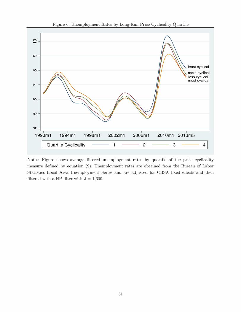
Other Regional Data. For specifications that examine the importance of local labor market

fluctuations, I use Metropolitan Statistical Area and Micropolitan Statistical Area unemployment

rates from the Bureau of Labor Statistics (BLS) Local Area Unemployment Statistics series.22 I

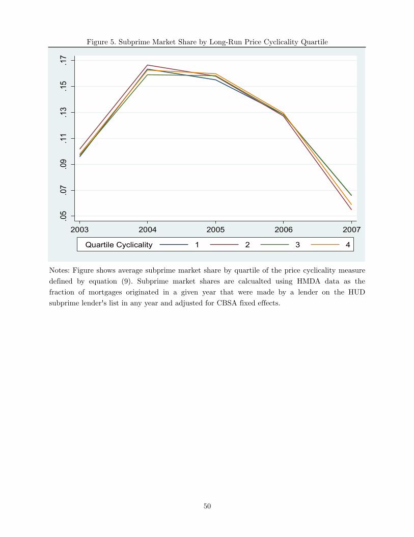
also use publicly available Home Mortgage Disclosure Act (HMDA) data to calculate the subprime

market share in a given CBSA ⇥ year by merging the lender IDs in the HMDA data with the

Department of Housing and Urban Development subprime lender list as in Mian and Sufi (2009).23

HMDA data discloses the census tract of each loan, which I allocate proportionally to CBSAs using

a crosswalk from tracts to zip codes and then from zip codes to CBSAs.

4 Estimation and Identification

4.1 Estimation

Arranging the data into a monthly panel with a dependent variable default icgt equal to unity if

existing mortgage i defaulted in month t, the likelihood h(t) of observing failure for a given monthly

observation must take into account the sample selection process. Namely, loans are not observed

after they have defaulted, so the likelihood of sampling a given observation is a discrete hazard,

which conditions on failure not having yet occurred. Suppressing dependence on X, the discrete

hazard is

h(t) ⌘ Pr(default icgt = 1)

= Pr(⌧ 2 (t� 1, t]��⌧ > t� 1)

=

ˆ t

t�1f(⌧)d⌧/S(t� 1)

= (F (t)� F (t� 1))/S(t� 1)

= 1� S(t)/S(t� 1)

where f(·) and F (·) are the density and cumulative density of ⌧ , the random variable representing

mortgage duration until failure, and S(·) = 1 � F (·) is the survivor function, the unconditional

21Available at http://www.census.gov/population/metro/data/other.html.22Available at http://www.bls.gov/lau/home.htm.23Using the HUD subprime lenders list to mark mortgages as subprime results in both false positives and false

negatives: lenders who self-designate as predominantly subprime certainly issue prime mortgages as well, and non-subprime-identifying mortgage lenders also issue subprime mortgages. See Mayer and Pence (2009).

13

probability that observed mortgage duration exceeds the given amount of time. Using the familiar

identity that S(t) = exp(�⇤(t)), where ⇤(·) is the integrated hazard function ⇤(t) =´ t0 �(⌧)d⌧ , I

can rewrite the likelihood of observing failure for a given observation to be

h(t��X) = 1� exp(�⇤(t) + ⇤(t� 1))

= 1� exp

✓�ˆ t

t�1exp(X(⌧)0�)�0(⌧)d⌧

◆

If time-varying covariates are constant within each discrete time period (for example if the observed

value of Xt represents the average of X(⌧) for ⌧ 2 (t� 1, t]),

h(t��X) = 1� exp

�� exp(X 0

t�)(⇤0(t)� ⇤0(t� 1))

�. (4)

where ⇤0(·) is the integrated baseline hazard ⇤0(t) =´ t0 �0(⌧)d⌧ .

Incorporating this likelihood of observing default icgt = 1, each month ⇥ loan observation’s

contribution to the overall log-likelihood is

`icgt = default icgt · log(h(t|Xicgt)) + (1� default icgt) log(1� h(t|Xicgt)). (5)

I can then estimate the hazard model parameters of equation (2) by Quasi-Maximum Likelihood in

a Generalized Linear Model framework where the link function G(·) satisfying h(t) = G�1(X 0

t�+ t)

is the complementary log-log function

G(h(t)) = log(� log(1� h(t))) = X 0t� + log(⇤0(t)� ⇤0(t� 1))| {z }

t

.

Estimating a full set of dummies t allows for the baseline hazard to be fully nonparametric à la

Han and Hausman (1990). The estimates of the baseline hazard function represent the average value

of the continuous-time baseline hazard function �0(·) over each discrete interval ¯�0t =´ tt�1 �0(⌧)d⌧

and are obtained as ˆ

¯�0t = exp(

ˆ t).24 Under the usual MLE regularity conditions, estimates of �

and will be consistent and asymptotically normal.

4.2 Identification

The proportional hazard model is identified—implying that the population objective function is

uniquely maximized at the true parameter values—under the assumptions that 1) conditional on

current covariates, past and future covariates do not enter the hazard (often termed strict exogene-

24Alternatively, t can be thought of as estimating a piecewise-constant baseline hazard function. As discussedabove in the context of the geographic fixed effects, the incidental parameters problem is not a concern here sinceincreases in sample size (the number of loans) would not increase the number of needing to be estimated.

14

ity), and 2) any sample attrition is unrelated to the covariates (Wooldridge, 2007).25 Stated in terms

of the conditional distribution F (·|·) of failure times ⌧ , the strict exogeneity and non-informative

censoring assumptions are met provided

F⇣⌧��⌧ > t� 1, {Xicgs, cis}Ts=1

⌘= F (⌧ |⌧ > t� 1, Xicgt)

where cis is an indicator for whether loan i was censored at time s. In principle, if lags or leads

of the covariates enter into �, the strict exogeneity condition can be satisfied by including them as

explanatory variables in the vector Xicgt.

An important form of censoring in mortgage data arises from borrowers paying back their mort-

gages in full. Mortgages that have been prepaid are treated as censored because all that can be

learned about their latent time until termination by default is that it is at least as long as the

observed elapsed time until prepayment. Technically, any such hazard model with multiple failure

types is a competing risks model, which can be generalized to accommodate the potential depen-

dence of one risk on shocks to another. Under the assumption there is no unobserved individual

heterogeneity in the default hazard (or that unobserved heterogeneity in the default and prepay-

ment hazards are independent at the individual level), competing risks models can be estimated as

separable hazard models with observations representing other failure types treated as censored.26

As in Gerardi et al. (2008), Sherlund (2008), Foote et al. (2010), and Demyanyk and Van Hemert

(2011), I adopt this approach and focus on estimation of the default hazard.27 In Appendix A, I

further validate this independent competing risks approach by verifying that my main results are

unaffected by allowing for unobserved heterogeneity in the default hazard.

Turning to causality, the key identifying assumption for the estimated coefficient µ in equation

(3) to be interpretable as the causal effect of the decline in property values is that fluctuations in

home prices and unobserved shocks to default risk are independent. To illustrate how the exogeneity

of X affects estimates of � in a hazard model setting, consider the case of time-invariant covariates

and no censoring. In this simplified setting, the exogeneity condition necessary for the maximum

likelihood estimates of the hazard model parameters to represent causal effects is that the probability

of failure (conditional on reaching a given period) is correctly specified in (2) and (3). Again, letting

25The linear-index functional form assumption that the effect of covariates on the hazard is linear in logs is notnecessary for identification and is made for the sake of parsimony and convenience in interpreting the coefficients.

26See Heckman and Honoré (1989) for a full discussion of identification in competing risks models.27The most well-known example of allowing for correlated default and prepayment unobserved heterogeneity is

Deng et al. (2000), who jointly estimate a competing risks model of mortgage termination using the mass-pointsestimator of McCall (1996).

15

⌧ be the random variable denoting the mortgage duration until failure, the formal condition is

lim

⇠!0+E

1 (⌧ 2 (t� ⇠, t])

⇠� �(Xicgt, t)

���X, ⌧ > t� ⇠

�= 0 (6)

where 1(·) is the indicator function. Analogous to omitted variables bias in a linear regression, this

condition would be violated if there were an omitted factor ! which affects default rates and is not

independent of X. In this case, misspecification leads to violation of the exogeneity assumption

because ! affects failure, is not in �, and survives conditioning on X. To see this, suppose that the

true instantaneous probability of default conditional on ⌧ > t� ⇠ is not �(X, t) but is

˜�(X,!, t) = exp(X� + !)˜�0(t).

In this case, the left-hand side of condition (6) evaluates to

lim

⇠!0+E

1 (t� ⇠ < ⌧ t])

⇠� �(X, t)

���X, ⌧ > t� ⇠

�= E

h˜�(X,!, t)

��Xi� �(X, t)

= Ehe! exp(X�)˜�0(t)

��Xi� �(X, t).

If ! and X are independent, then the exogeneity condition becomes

Ehe! exp(X�)˜�0(t)

��Xi� �(X, t) = exp(X�)E [e!] ˜�0(t)� exp(X�)�0(t).

Thus, the presence of independent ! simply scales the estimate of the baseline hazard function. In

other words, the baseline hazard function estimated without controlling for ! will be estimating

E [e!] ˜�0(t)—but the estimation of the slope coefficients will be unaffected and the exogeneity con-

dition of equation (6) will hold in expectation. However, if ! and X are not independent, then the

omission of ! leads to a violation of equation (6), and estimated � will not represent the marginal

effect of X on default, as discussed in Section 5.2 below.28

4.2.1 Unobserved Heterogeneity

In the general case, even unobserved heterogeneity that is independent of the controls will affect

the conditional distribution of ⌧ |X (and hence the estimated coefficients), a common obstacle in

nonlinear panel models. Lancaster (1979) introduced the Mixed Proportional Hazard (MPH) model

where the heterogeneity enters in multiplicatively (additively in logs).29 Conditional on unobserved28Estimating a proportional hazard model with no censoring and time-invariant covariates is equivalent to a

linear regression of log duration on the covariates (Wooldridge, 2007). This illustrates why this special case permitsunobserved heterogeneity provided it is independent of the covariates; in a linear model, additive unobservables affectthe consistency of the parameter estimates only if they are correlated with the covariates.

29Elbers and Ridder (1982) showed that the MPH model is identified provided there is at least minimal variationin the regressors.

16

heterogeneity ", the hazard function becomes

�(t|Xicgt, "i) = exp(X 0icgt� + "i)�0(t). (7)

The literature on unobserved heterogeneity in duration models has broadly found that ignoring

unobserved heterogeneity biases estimated coefficients down in magnitude. Intuitively, the presence

of " induces survivorship bias—loans with low draws of " last longer and are thus overrepresented

in the sample relative to their observables. Individuals whose observable characteristics put them

at a high ex-ante risk of default and yet have lengthy durations are likely observed in the sample

because they have low unobserved individual-specific default risk (high latent quality). The nega-

tive correlation between X and " induced by the sample selection process can prevent consistent

estimation of �.

Equation (7) pins down the conditional distribution F of latent failure times ⌧ to be

F (⌧ |Xicgt, "i) = 1� exp (�⇤((t|Xicgt, "i))

where ⇤(·|X, ") is the integrated hazard. Specifying the distribution of " to have cumulative distri-

bution function G(·), the distribution ˜F (⌧ |Xicgt) of ⌧ |X is then obtained by integrating out ":

˜F (⌧ |Xicgt) =

ˆ 1

�1F (⌧ |Xicgt, "i)dG("i).

Finally, the modified likelihood ˜h(t|X) of observing failure at time ⌧ 2 (t� 1, t] is

˜h(t|X) = 1� ˜S(t|X)/ ˜S(t� 1|X) (8)

where the new survivor function is denoted ˜S(·|X) = 1 � ˜F (·|X). Estimation then proceeds by

replacing h(·|X) with ˜h(·|X) in the log-likelihood expression of equation (5). In Appendix A, I verify

that my results are robust to the presence of independent unobserved heterogeneity by specifying

" ⇠ N (0,�2) so that G(") = �("/�), where �(·) is the standard normal cumulative density function.

4.3 Isolating Long-Run Variation in Housing Price Cycles

One example of an omitted factor that may be correlated with X is the expansion of subprime credit,

which may initially increase prices as a positive shock to the demand for owner-occupied housing,

as suggested by Mayer and Sinai (2007), Mian and Sufi (2009), Pavlov and Wachter (2011), and Di

Maggio and Kermani (2014). If the credit supply expansion leads to a decrease in the quality of

the marginal borrower, prices will eventually fall as these riskier borrowers default. Their defaults

17

will depress prices in at least three ways: from a positive shock to the supply of owner-occupied

housing on the market, from negative foreclosure externalities (see Hartley, 2014 and Campbell et

al., 2011), and by changing the home-price beliefs of buyers and lenders.30 Thus, the expansion of

subprime credit may be an omitted variable that directly affects both defaults (by decreasing the

quality of the marginal subprime borrower) and prices, potentially leading to a spurious estimated

relationship between prices and defaults. A related worry from the perspective of the exogeneity

condition in equation (6) is that areas with the strongest price declines are also likely the areas hit

hardest by the recession. If a negative employment shock simultaneously causes both defaults and

price declines, then local labor market strength may be an important omitted variable that biases

the estimates towards finding an effect of prices on default.

To address these endogeneity concerns, I develop an instrument that isolates the long-run com-

ponent of each Core Based Statistical Area’s (CBSA) price cycle and is arguably independent of

contemporaneous shocks to prices or default rates, e.g. from credit or labor market fluctuations.

The CoreLogic repeat-sales price index for each CBSA, discussed in greater detail above, provides

a measure of the relative level of nominal home prices in a given CBSA ⇥ month, denoted here

as HPIgt. Sinai (2012) notes that a similar set of metropolitan areas had large or small 1980s

and 2000s price cycles. There could be several drivers of house-price persistence, including local

demographics, housing supply elasticity, migration elasticity, and industry composition. For the

instrument to be valid, whatever leads a given area to have a consistently cyclical housing market

must be unrelated to the subprime credit expansion, as I describe and test in Section 5.2.2 below.

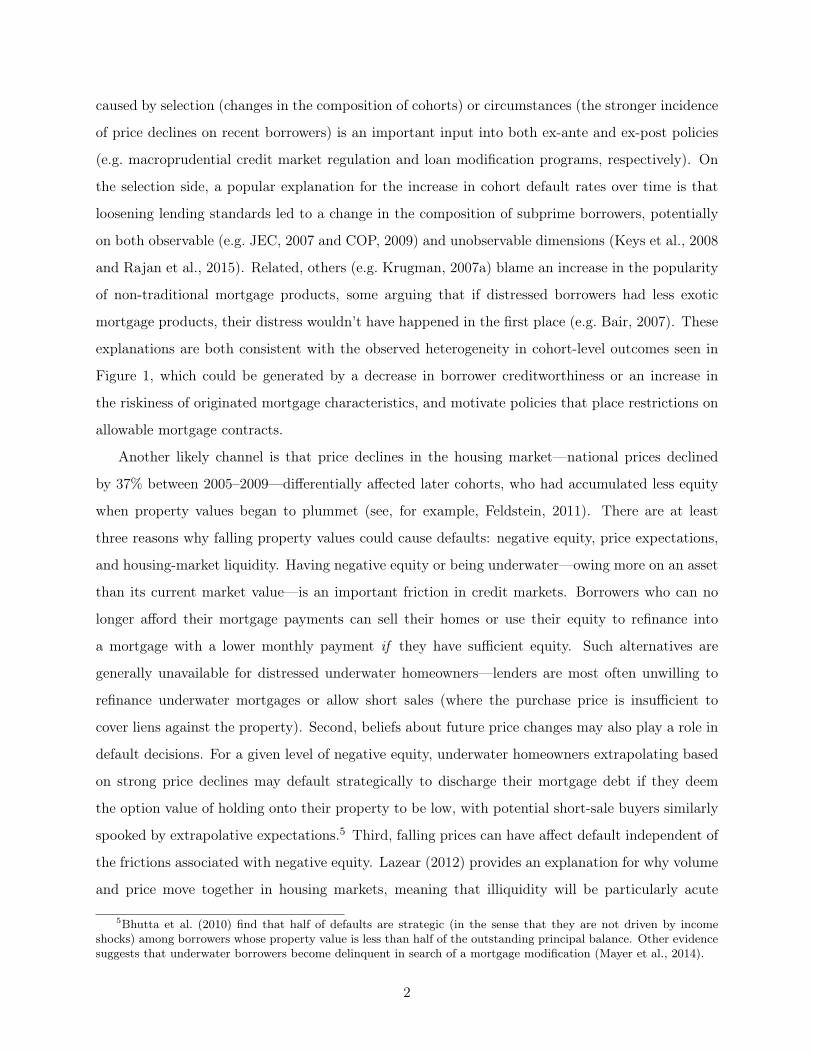
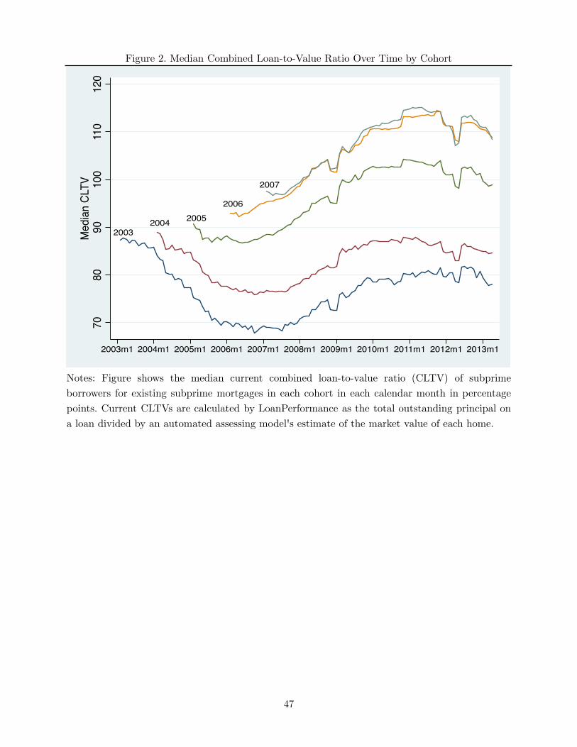
To measure this persistence, I determine the portion of a CBSA’s price cycle that is predictable

using only the historical cyclicality of that city. First, I form a summary measure �Pg quantifying

the long-run cyclicality of CBSA g defined as the standard deviation of monthly changes in the

CoreLogic repeat sales home price index from 1980-1995

�Pg ⌘

1

T � 1

X

t2T(�HPIgt ��HPIg)

2

!1/2

(9)

where T = 180 is the number of months over which the standard deviation is calculated; T is the

30Dagher and Fu (forthcoming) provide an example of the mechanism behind such an expansion: counties thathad significant entry of non-bank mortgage lenders had stronger growth in credit and prices, as well as strongersubsequent increases in defaults and decreases in prices. Brueckner et al. (2012) offer a model of how price increasescould fuel lender expectations and further credit expansion. Berger and Udell (2004) also discuss empirical evidenceof underwriting standards deteriorating during a credit expansion. Baron and Xiong (2015) and Lopez-Salido etal. (2015) offer time series evidence that credit expansions are historically associated with economic declines withina few years.

18

set of months from January 1980 to December 1995, inclusive; �HPIgt = HPIgt �HPIgt�1; and

�HPIg is the average value of �HPIgt for CBSA g and t 2 T .31 Plotting the 1980-1995 HPI paths

shows that high-�P areas had more pronounced boom-bust cycles and that the actual timing of each

CBSA’s house price cycle was unrelated to �P , consistent with the asynchronicity of regional price

fluctuations during that time period. Figure 3 shows the average value of the CoreLogic repeat sales

home price index by quartile of �P . The persistence in price volatility isolated by the first stage is

visible: the average price cycle in the late 2000s was much more pronounced for CBSAs that had

stronger price cycles in the 1980s, that is, higher quartiles of �P have monotonically stronger price

cycles.

5 Results

5.1 Results Treating Price Changes as Exogenous

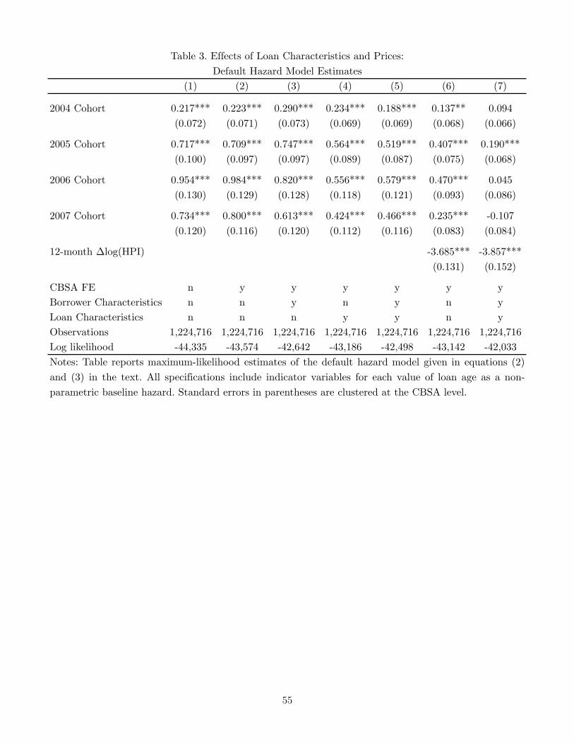
Table 3 reports estimates of equation (2) using the estimator described above, treating price changes

as exogenous to offer initial estimates of the relationship between price changes, underwriting stan-

dards, and cohort-level differences in default rates. I cluster all standard errors at the CBSA level to

account for area-specific shocks to the default rate in inference. All specifications include nonpara-

metric controls for the baseline hazard function.32 Column 1 includes only cohort fixed effects to

quantify the pattern of declining cohort-level performance from Figure 1 in a hazard-model frame-

work. These coefficients can be interpreted as the change in the log hazard rate and imply, for

example, that subprime loans in the 2007 cohort had a default hazard 73 log points greater than

the 2003 cohort (the omitted category). These unadjusted cohort coefficients are large and precisely

estimated, implying that the probability of a 2005–2007 cohort mortgage defaulting in any given

month conditional on the mortgage having survived to that month is more than twice as high as

2003 cohort mortgages. Column 2 adds fixed effects for each CBSA in the sample (568 fixed ef-

fects) to verify that cohort differences are not driven by the geographic composition of later cohorts.

Conditioning on CBSA fixed effects does not materially affect the estimated differences in cohort

default hazards.31I calculate the standard deviation of the first differences in the HPI variable to emphasize the importance of the

(low-frequency) price cycle. CBSAs with high variance of HPI in levels (as opposed to high �HPI) could simply beareas that had sustained price growth or high-frequency volatility.

32The baseline hazard controls consist of an indicator variable for each possible value of loan age from 1–70 months,with the final indicator variable also turned on for all values of loan age exceeding 70 months. The estimated baselinehazard functions resemble the hump-shaped baseline hazards of Deng et al. (2000) and are available from the authoron request.

19

Columns 3 and 4 add borrower characteristics and loan characteristics, respectively, as detailed

in Section 3. The coefficients on these credit risk factors (available on request) all have intuitive

signs. Borrowers had higher default rates if they lacked full income documentation, were not owner-

occupants, or had lower FICO scores and higher DTI ratios. Mortgages defaulted more frequently

if they were non-fixed rate mortgages, had higher CLTVs or interest rates, or were accompanied by

additional liens. Column 3, which includes only borrower characteristics, shows that the adjusted

default hazard of earlier cohorts is slightly higher than in column 1, suggesting that, relative to 2003

borrowers, 2004 and 2005 subprime borrowers underperformed relative to what would be expected

based on their individual attributes. For 2006–2007 cohorts, the differential default hazard is lower

than in column 1, although the average decrease in the estimated cohort differences of columns

1 and 3 is approximately zero and the individual cohort differences between columns 1 and 3 are

statistically insignificant. The inability of borrower characteristics to substantively explain the

cohort-level differences is not surprising given the summary statistics reviewed above showing that

the mean observable attributes of borrowers are not changing much across cohorts.33 The results

of column 4 tell a different story: including controls for loan characteristics and not borrower

characteristics explains on average 24% of the unadjusted cohort effects estimated in column 1. This

suggests that the loan characteristics that were changing across cohorts (and the change in borrower

unobservables that they represent) were an important driver of defaults. Conditioning on both

borrower and loan characteristics together in column 5 reduces the residual cohort heterogeneity

(i.e. the column 4 coefficients relative to the column 1 coefficients) by an average of 29%.

To get a sense of which covariates are most important in explaining the cohort pattern, I esti-

mated the specification of column 5, leaving out one characteristic at a time. Three characteristics

stand out as contributing substantially to the attenuation of the estimated cohort effects: the bal-

loon and interest-only dummies and the loan interest rate. As the interest rate should represent

everything that the market knew about the riskiness of the loan, its importance reenforces that

priced observables are important in predicting the cohort-level default pattern. The importance

of the balloon and interest-only indicators is consistent with Table 2, which showed that balloon

mortgages and interest-only mortgages were the two product characteristics that changed the most

across cohorts and thus had the strongest potential to explain cohort-level defaults.

Column 6 drops all borrower- and loan-level covariates and instead controls for the 12-month

33While individual borrower characteristics do not explain much of the differences in default rates across cohorts,they are individually strong predictors of default, as evidenced by the large increase in the log likelihood value betweencolumns 2 and 3.

20

change in log of the CoreLogic repeat-sales Home Price Index (HPI), defined at the CBSA-level as

� log(HPIicgt) ⌘ log(HPIicgt)� log(HPIicgt�12) (10)

where HPIicgt is the value of the CoreLogic repeat-sales price index for CBSA g in the calendar

month corresponding to loan i having a duration of t.34 This variable is a strong predictor of default.

The coefficient on the 12-month change in log HPI implies that properties experiencing the 75th

percentile 12-month price change (+5%) would have a 33% lower hazard than properties exposed

to the 25th percentile 12-month change in prices (–5%), corresponding to an approximately one

percentage point decrease in the annual default rate. Controlling for the 12-month change in prices,

the cohort effects in column 6 are lower than the estimates in column 5, showing that price changes

in the most recent 12 months seem to be more closely related to observed cohort heterogeneity than

borrower and loan characteristics. The residual differences in default rates across cohorts decrease

on average by 50% (depending on the cohort) relative to the baseline cohort coefficients in column 1.

Controlling for both borrower and loan characteristics and price changes leaves little cohort-

level heterogeneity unexplained. The estimates in column 7 of the latent quality of each cohort

(i.e. the portion of cohort outcomes not attributable to price changes or individual-level controls)

are statistically insignificant with the exception of the 2005 cohort. While statistically significant,

more than 70% of the unadjusted estimate of the difference between the 2003 and 2005 cohorts

(column 1) is explained by prices and observables.

These results illustrate that both observable loan characteristics and prices play important roles

in explaining the rise in default rates across origination cohorts, together explaining on average 95%

of the cohort disparities in column 1.35 In particular, places where price declines are greater have

higher default rates, and the incidence of these price declines is disproportionately borne by later

cohorts. I now turn towards developing causal estimates of the impact of prices on default behavior.

34I index HPI by i as well to emphasize that in my notation t refers to event time (i.e. loan age). Even thoughHPI only varies by CBSA ⇥ calendar month, for example, not all six-month old (t = 6) mortgages in CBSA g havethe same HPI value.

35The additional explanatory power gained from controlling for prices and characteristics simultaneously suggeststhat there are important interactions between prices and loan and borrower characteristics. One implication ofthe proportional-hazard framework is that interactions between the covariates is implicit: the cross-partial of thehazard function with respect to two covariates is the hazard function times the product of the two coefficients onthe covariates. For example, this multiplicative relationship between the covariates allows for price declines to havelarger effects for riskier borrowers.

21

5.2 Control Function Estimation

As discussed above, the interpretation of these results as causal requires the assumption that changes

in the average default risk of a given area are not the cause of local price changes. Reverse causality

is one concern: because defaults themselves cause price declines as discussed above, the exogeneity

assumption is likely to be violated by any regional shock to default risk. Omitted variables (such as

local growth in subprime credit) that affect both defaults and prices also confound the estimates: the

housing demand shock resulting from the credit expansion may initially increase prices, and even-

tually a higher share of riskier borrowers may exacerbate price declines (Di Maggio and Kermani,

2014). In this way, if price changes are endogenous to subprime penetration and subprime growth

reduces unobserved borrower quality, then the estimation would misattribute much of the increase

in defaults to price changes instead of to differences in unobserved cohort quality resulting from

the credit expansion. Fluctuations in local labor market conditions are also an important omitted

variable. Adverse local labor shocks may simultaneously decrease prices (negative demand shock

for owner-occupied housing) and increase defaults (negative income shock to existing mortgagors).

On the other hand, if there is a direct impact of falling collateral values on default, then even price

declines not caused by local labor market changes or credit expansions will explain a substantial

portion of the rise in subprime defaults. Moreover, the reverse causality story could conceivably

bias downwards the magnitude of the elasticity of default with respect to prices. If both channels

are present, i.e. if price declines and defaults cause each other, then if the magnitude of the defaults

causing price declines channel is smaller than the price declines causing defaults channel, the esti-

mates that treat price declines as exogenous will confound the two and be smaller than estimates

that isolate the (larger) causal effects of price declines.

The potential for changes in local home prices to themselves be a function of contemporaneous

shocks to the default hazard through subprime lending or employment shocks necessitates instru-

menting for prices. To instrument in this nonlinear setting, I use the control function approach (see

Heckman and Robb, 1985). This estimator involves conditioning on a consistent estimate of the

endogeneity in the endogenous explanatory variable and in a linear model is equivalent to two-stage

least squares.

To see why the control function approach solves the endogeneity problem, suppose again that

there exists an omitted variable ! in the default hazard equation, which is not independent of X.

22

Labeling the true hazard function ˜�(·), if

˜�(X,!, t) = exp(X� + !)�0(t) = e! exp(X�)�0(t).

If I do not control for ! in estimating this model, the resulting � coefficients will be estimating a

different object than the marginal effect of X on the log hazard. Formally, the exogeneity condition

introduced in equation (6) above now fails:

E⇥default t � �(X, t)

��X, ⌧ > t⇤

= Eh˜�(X,!, t)

��Xi� �(X, t)

= E⇥e!��X⇤�(X, t)� �(X, t)

= [exp(X� + f(X))� exp(X�)]�0(t)

6= 0

where E(e!��X) ⌘ f(X) because X and ! are not independent. Thus, under misspecification, the

coefficients on X will not converge to the marginal effect of X on the log hazard and instead combine

both the direct effect of X on default and the indirect effect of ! on default after projecting onto X.

Conditioning on an estimate of the endogenous component of X solves this problem. Let the

right-hand side endogenous variable be specified as

�Prices = Z1⇧1 + Z2⇧2 + v

where the endogeneity problem arises because v and ! are not independent. The key identifying

assumption is that the instruments Z1 and included right-hand side controls Z2 (the elements of X

apart from �Prices) are independent from v and !. Conditioning on v then satisfies the exclusion

restriction

E⇥default t � �(X, v, t)

��X, v, ⌧ > t⇤

= Eh˜�(X,!, t)

��X, vi� �(X, t, v)

= E [e!|v]�(X, t, v)� �(X, t, v)

= (exp(g(v))� exp(⇢1 + ⇢2v)) exp(X�)�0(t)

where g(v) ⌘ E(e!��v).36 If the conditional expectation E(e!

��v) = exp(⇢1+⇢2v), then this condition

will hold, and controlling for a consistent estimate of v will be sufficient to allow estimation of the

partial effect of X on the log hazard. This will be satisfied exactly under the parametric assumption

that ! conditional on v is distributed normally: if !|v ⇠ N (⇢2v, 2⇢1) then e!|v is distributed log

36In addition to the exogeneity condition that (Z1, Z2) are independent of (!, v), identification requires the usualrelevance condition. If there is only a weak first stage in the sense that ⇧1 ⇡ 0, then conditioning on v and Z2 willsoak up all of the variation in �Prices, and � will not be identified.

23

normally with mean E(e!��v) = exp(⇢1 + ⇢2v). If the conditional distribution of ! given v is

non-normal, then controlling linearly for v in the hazard model relies on the quality of the linear

model as a first-order approximation to the conditional mean function. As a robustness check,

Appendix B considers third- and fifth-order polynomial approximations to the log of the conditional

expectation function, e.g. log (E(e!|v)) =

P5k=0 ⇢kv

k and finds that the results are insensitive to

this semiparametric flexibility.

5.2.1 First Stage

The instrument set for the price change variable is the long-run cyclicality measure �Pg interacted

with calendar-month indicator variables. The first stage for the 12-month price change is then

� log(HPIicgt) =X

s

⇡s�Pg · 1(s = t+ t0(i)) + Z 0

2,icgt⇡2 + vicgt (11)

where Z2,icgt contains the same covariates as equation (3) above—cohort effects, geographic fixed

effects, loan and borrower characteristics, and the nonparametric baseline hazard function to ensure

that predicted values from equation (11) are orthogonal to the other controls in equation (2). The

function t0(i) evaluates to the calendar time of loan i’s origination date, and the ⇡s coefficients are

turned on when the observation on loan i at t months after origination corresponds to calendar

month s.

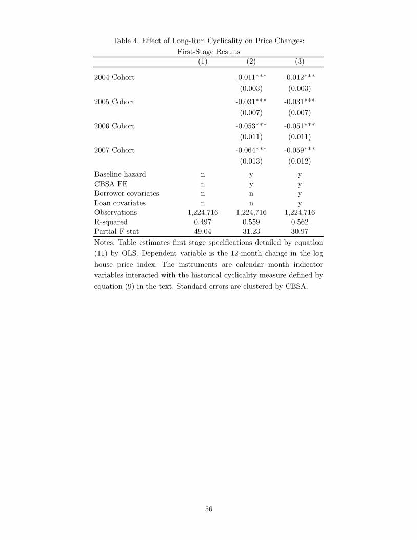
Table 4 reports the results from estimating first-stage equation (11) by OLS with standard errors

clustered at the CBSA level. Column 1 includes just the instrument set and no other controls. The

statistical relationship between actual price changes and the interactions between the cyclicality

measure and calendar time is strong—the instruments explain 50% of the variation in twelve-month

CBSA-level home price changes. Adding controls for the baseline hazard and CBSA fixed effects

in column 2 improves the overall fit slightly (R2 increases to 0.56). Including loan and borrower

characteristics in column 3 does not affect the partial F -statistic, which tests the joint hypothesis

that all of the coefficients on the instrument set are zero, suggesting that weak instruments are not

a problem in this setting.37

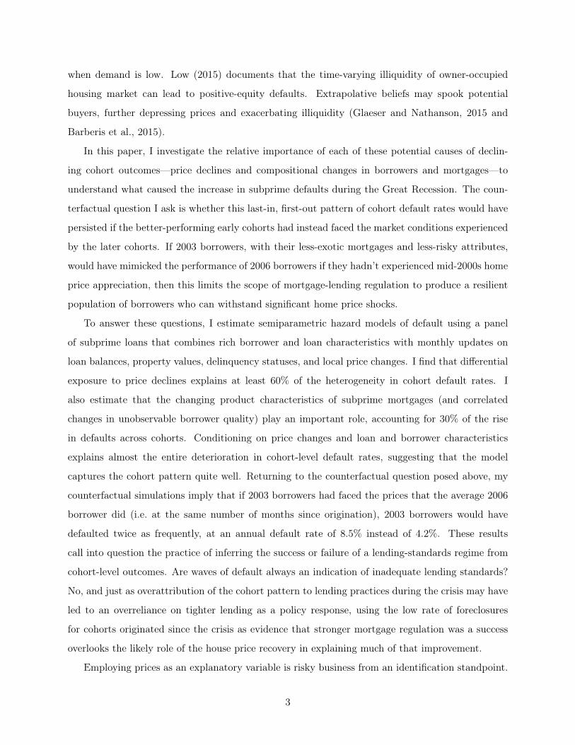
To provide intuition for how this instrument operates, I compute counterfactual price indices by

regressing log home-price indices on geographic fixed effects and an interaction of �Pg with calendar-

37The cohort coefficients in columns 2 and 3 illustrate that later cohorts were exposed to stronger price declinesthan earlier cohorts, in part by virtue of selection—younger loans have had less time to prepay and are thus morelikely to be extant and exposed to recent price declines.

24

month indicators as follows

log(HPIgt) = ↵g +X

s

⇡s�Pg · 1(s = t) + ugt (12)

where HPIgt is the value of the CoreLogic home price index in CBSA g in calendar month t.

The estimated ⇡̂s shift the baseline log HPI of each CBSA (↵g) according to the cross-sectional

relationship each calendar month between prices and 1980s price volatility.38 Predicted valuesd

logHPIgt from this regression provide an alternative time series of home prices in geography g

based on the quasi-fixed tendency of home prices in geography g to cycle up and down.

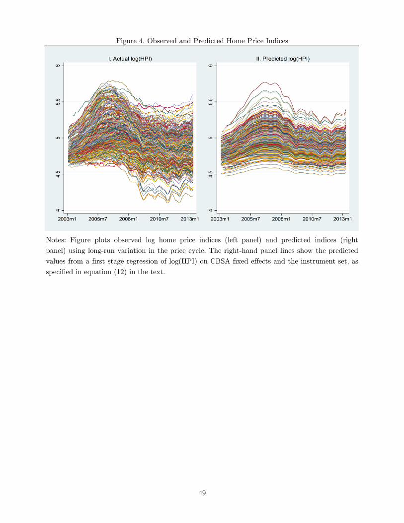
Figure 4 shows the actual log home price series for 2003–2013 (left-hand panel) along with

predicted values from equation (12) (right-hand panel). The left-hand panel shows that the actual

HPI series are characterized by idiosyncratic deviations from the national trend, i.e. price shocks

that potentially arise from such factors as local credit expansions and local labor market fluctuations

that may also independently affect default rates. It is precisely the effects of these types of shocks

from which the instrument is designed to abstract. Because nothing in equation (12) allows for

differential price trends across CBSAs, the predicted time series in the right-hand panel all change

in the same direction each month, differing only in the magnitude of the price change depending on

their historical price volatility. To the extent that the actual price paths reflect time-varying local

housing market changes, each line on the right is an estimate of the counterfactual price path that

might occur absent local price shocks that are potentially driven by factors that also affect local

default risk. Intuitively, my empirical strategy instruments for the actual price series on the left

with the predicted price series on the right.

5.2.2 Exclusion Restriction

The necessary exclusion restriction for the control-function results to be unbiased estimates of the

causal effect of price changes is the independence of the size of a CBSA’s 1980s price cycle (�Pg ) from

any other factors that affect default (besides prices). Note that with CBSA fixed effects, it is not

a threat to identification if cyclical areas are fundamentally different from acyclical areas in some

time-invariant way (e.g. an inherently risky area may always have both higher defaults and larger

price swings). However, this exclusion restriction would be violated if pro-cyclical housing-market

38Note that equation (12) does not control for main effects for each date. While this loads the national month-to-month variation in home prices onto the ⇡t, date effects—the embodiment of the rise in subprime defaults—arethe very object the hazard model seeks to explain. As they are not instruments and they do not belong in thesecond-stage, I purposefully omit them here.

25

areas also (high �Pg ) have pro-cyclical trends in the credit risk of borrowers. For example, if high-�Pgareas had more rapid subprime growth, then �Pg may proxy for changes in unobserved borrower

quality in CBSA g. Similarly, if high-�Pg areas have greater unemployment rate fluctuations, these

adverse shocks to local aggregate demand could increase defaults (through an income shock) and

decrease prices (through a demand shock).39

Figures 5 and 6 offer graphical evidence that subprime shares and unemployment rates—

adjusting both for CBSA fixed effects—did not vary systematically with �Pg . The relevant period

is different for each endogeneity concern. Figure 5 plots the annual adjusted subprime share of

HMDA-covered mortgages originated in 2003–2007 by quartiles of �Pg . There is no apparent rela-

tionship between �Pg and subprime originations—places with historically large price cycles do not

seem to have been any more prone to subprime credit expansion.40 Figure 6 plots average smoothed

unemployment rates from 1990–2013 by �Pg quartile. While areas that had cyclical housing mar-

kets from 1980-1-1995 had cyclical contemporaneously cyclical labor markets, evidenced by the top

quartile having the strongest unemployment cycle in the early 1990s, Figure 6 shows that the top

quartile of �Pg had around a 1 percentage point lower unemployment rate in recession than the

bottom quartile.

Regression versions of these tests tell a somewhat different story. I test whether there is a

“first stage” for the annual subprime share of all residential mortgage originations and the monthly

unemployment rates by re-estimating equation (11), replacing the dependent variable with the

subprime share of mortgages originated in each cohort and with the monthly unemployment rate

in each CBSA. Consistent with Figure 5, the estimated coefficients ⇡̂t for the subprime share first

stage are statistically insignificant and nearly zero, showing that loans from areas with higher

historical price volatility were no more likely to have been originated during a relatively large

subprime credit expansion. The estimated ⇡̂t in the unemployment regression, however, mimic

the national trends in the unemployment rate, with historically cyclical areas having differentially

lower unemployment rates leading up to the recession and more quickly rising unemployment rates

thereafter. This provides evidence that areas with historically cyclical housing markets may also

have cyclical labor markets and that national labor market changes load onto the instruments.

Below, I verify the robustness of my control-function estimates to controls for changing labor market

39Note that Mayer (2010), Mian (2010), and Mian and Sufi (2014) argue that price declines first caused unem-ployment in the recent recession.

40Note that the same fact is not true about the relationship between subprime originations and the size of the 2000sprice cycle—areas that originated the highest share of subprime mortgages indeed had stronger (contemporaneous)price cycles, consistent with Di Maggio and Kermani (2014).

26

conditions. An important caveat is that housing market changes can also affect labor markets (see

Mayer, 2010, Mian, 2010, and Mian and Sufi, 2014). To the extent that the observed correlation

between my instrument and labor market outcomes is an effect of the price cycle and not vice

versa, then the instrument captures the total causal effect of price changes. However, because of

the difficulty in ascertaining which caused which, I treat the relationship between the instrument

and unemployment as a threat to validity. To account for this unemployment channel, I present

additional control function specifications below that also control for the unemployment rate, thereby

isolating the variation in prices that is not correlated with local labor market shocks or local subprime

expansion.41

5.2.3 Control Function Results

Table 5 employs a nonlinear control function approach, which accounts for the endogeneity of price

changes to the credit expansion by controlling for the first-stage residuals v̂icgt in the default hazard

index

X 0icgt� = �c +W 0

B,i✓B +W 0L,i✓L + µ ·�Pricesicgt + v̂icgt + ↵g (13)

where v̂ = � log(HPI)� d� logHPI and d

� logHPI is fitted from equation (11). To account for the

generated regressor problem in inference (Pagan, 1984 and Murphy and Topel, 1985), I also report

bootstrapped standard errors in brackets below clustered standard errors. The generated regressor

problem arises because v depends on an unknown parameter vector ⇡, as seen in equation (11).

Consistently estimating ⇡ in a first stage to generate v̂ does not affect the consistency of parameters

estimated in (13). However, by treating v̂ as fixed, i.e failing to account for the correlation between

the estimation error in ⇡̂ and the error in estimating �, the usual asymptotic standard errors will

generally be understated unless = 0. The block bootstrap solves this by mimicking the data-

generating process. In this setting, individual mortgages are resampled with replacement instead

of month ⇥ loan observations being drawn with replacement as would be the approach of standard

nonparametric bootstrap. The two stages (estimating v̂ from (11) and estimating equation (13)) are

then run on each bootstrapped sample and the resulting bootstrap standard errors are the empirical

standard deviation of each element of � across 200 bootstrap replications.

41The relationship between home price cyclicality and labor market cyclicality hints at the economics behind whysome areas may be more cyclical than others. Areas with high housing supply elasticity, potentially arising fromgeographic constraints, land-use regulations, or credit market regulations, could be pro-cyclical in both markets.Similarly, areas with an industry mix that makes them particularly sensitive to recessions or commodity price shocksmay experience coincident fluctuations in housing and labor.

27

Column 1 of Table 5 repeats column 6 of Table 3 for reference, controlling for the 12-month

change in prices and not conditioning on borrower or loan observables WB and WL. Column 2

additionally controls for the residuals v̂icgt, estimated from OLS on equation (11) (omitting loan

and borrower characteristics in the construction of the residuals). The coefficient on the price

change variable is still large and significant—borrowers experiencing a 1% price decline over the

previous year have a 4.4% higher conditional probability of default. The adjusted cohort differences

are smaller in column 2 than column 1, meaning that after accounting for endogeneity, the role of

prices in explaining the default pattern is larger. Comparing column 2 to the benchmark differences

in cohort performance measured in column 1 of Table 3, controlling and instrumenting for prices

without controlling for borrower or loan characteristics explains 60% of the difference in unadjusted

cohort outcomes. The statistical significance of the coefficient on the residual is equivalent to a

Hausman test for the endogeneity of price changes, similar to a Rivers and Vuong (1988) test for

endogeneity in a probit model, confirming that price changes are endogenous.

To address the correlation between the instrument and local labor market shocks, column 3 also

controls for the monthly CBSA unemployment rate, measured in percentage points.42 Conditional

on the covariates in the column 3 specification, a one percentage point increase in the local unem-

ployment rate is associated with a decrease in the default hazard of 2%. The slight increase in the

magnitude of the coefficient on prices from –4.4 to –4.5 suggests that the price results are not driven

by correlation between price shocks and local labor shocks.43 The estimated differences in cohort

quality in column 3 do not differ substantively from column 2.

The bootstrapped standard errors in columns 2 and 3 (in brackets) are in general larger than

the standard errors clustered at the CBSA level (in parentheses), representing a high variability in

the estimated residuals v̂ across bootstrap samples. However, the relative stability of the coefficient

magnitudes suggest that the patterns described above hold at least qualitatively. Further, because

the asymptotic standard errors are correct under the null hypothesis H0: = 0, the conventional

t-statistic on the fitted residuals is still a valid test of exogeneity.

The next three columns additionally control for borrower and loan characteristics. The estimated

cohort effects in these specifications capture the latent quality of each cohort, i.e. the heterogeneity

in cohort-level default rates not explained by ex-ante observable quality or price changes. Column

42The sample size decreases slightly in specifications controlling for unemployment rate because of one CBSA forwhich BLS does not estimate monthly unemployment rates.

43The counterintuitive sign on the monthly unemployment rate, which could be driven by the reliance of mortgagemodification programs on observable employment status, is statistically significant but very small in magnitude.

28

4 repeats column 7 of Table 3 for convenience, controlling for price changes in addition to all of the

other controls. Column 5 reports control function estimates of this specification. The coefficient

on the price change variable increases in magnitude from –3.9 to –4.6 (see below discussion). The

coefficient on the endogenous portion of the 12-month change in home prices is again positive

and significant. Importantly, I cannot reject that each of the cohort latent quality measures is

statistically indistinguishable from zero with the exception of the 2005 cohort, as before. Moreover,

the estimated cohort effects in column 4 are each smaller than those in column 3 which treat prices

as exogenous. Column 6 again controls for the monthly unemployment rate. The magnitude of

unemployment on default is almost identical as in column 3, suggesting that the unemployment

rate does not interact meaningfully with loan and borrower characteristics. The price effects—

both the main effect and the residuals—are strengthened by the inclusion of the unemployment

rate control, although this difference is not statistically significant. Each of the cohort effects is

attenuated slightly from column 5. The specifications in columns 5 and 6 both explain 95% of the

unadjusted differences in cohort default rates in column 1 of Table 3.

Interestingly, the bootstrapped standard errors in columns 5 and 6 are much more similar to

their asymptotic (clustered) counterparts than the bootstrapped standard errors of columns 2 and

3. Unlike columns 2 and 3, the results of columns 5 and 6 are robust to bootstrapping the standard

errors. This suggests that much of the instability of the bootstrap estimates in columns 2 and 3 is

driven by not controlling for loan and borrower characteristics, which explain a substantial amount

of individual heterogeneity in default risk.

A consistent pattern in Table 5 is that instrumenting (columns 2, 3, 5, and 6) increases the

magnitude of the estimated effect of price changes relative to not instrumenting (columns 1 and 4),

with the estimated coefficient ̂ on the residuals positive. While the partial effect of an endogenous

price shock v on the log of the default hazard—equal to µ̂+ ̂ because the residuals enter into the

X� index through both �Prices and v—is strongly negative (as expected) in each specification,

the effect of an exogenous change in prices captured by µ̂ alone is much greater. This is consistent

with some degree of treatment effect heterogeneity—locales emphasized by the instrument that

have experienced large price declines historically may be more sensitive (i.e. their default behavior

more elastic) to current price declines. Alternatively, if the feedback from defaults to prices (reverse

causality) is weaker than the impact of prices on defaults, then the estimates that do not instrument

and thus conflate both channels will be smaller than the control-function estimates that isolate the

direction of causality from prices to defaults. Finally, instrumenting may solve an errors-in-variables

29

problem with �Prices—CBSA-level HPI estimates may be an imperfect proxy for the property

value shock faced by an individual borrower in a given CBSA.

The control function results of Table 5 and Appendix Table 2, which addresses the possibility that

the conditional distribution of the endogeneity is misspecified and is discussed in Appendix B, are

consistent with the results of Table 3, providing evidence that there is a large causal effect of price

declines on defaults. Even after accounting for the simultaneous relationship between collateral

values and default risk, there is little evidence that unobserved borrower quality (i.e. borrower

heterogeneity not captured by observable loan and borrower characteristics) declined across 2003–

2007 cohorts.

In summary, this section was concerned with determining how much of the pattern across orig-

ination cohorts in default rates was due to differences in the observed characteristics of mortgage

borrowers in each cohort—both the creditworthiness of the individual borrowers and the character-

istics of their mortgages—and differences in their exposure to price declines. The results confirm

that prices and mortgage characteristics are both important, with price changes causally explaining

at least 60% of the increase in cohort default rates.

6 Mechanisms

Through what mechanisms did price changes affect default rates? Below, I estimate the causal

effect of negative equity on defaults and to what extent this explains the increase in defaults across

subprime borrower cohorts. The intuition offered in Section 1 focused on the differential effect of

price declines on later cohorts in pushing them underwater, as seen in Figure 2. In contrast to

underwater homeowners, positive-equity but distressed borrowers (i.e. borrowers unable to make

their monthly mortgage payments) have two main alternatives to default. First, if interest rates

have gone down since origination or if borrowers qualify for a lower interest rate because they

have more equity from accumulated price appreciation or paid-down mortgage principal, they can

refinance into a mortgage with a lower monthly payment using the new mortgage to repay the

original one.44 Second, homeowners with positive equity can sell their home and use the proceeds

to pay off their outstanding mortgage debt and move into a more affordable housing situation.

Neither of these options is readily available to distressed borrowers who are underwater. Lenders

are normally unwilling to originate a refinance mortgage to someone who does not have at least 20%

44Relatedly, a home equity line of credit can also be used by positive-equity borrowers to borrow additional fundssecured by unrealized capital gains. These funds can be used to temporarily make mortgage payments.

30

equity, let alone negative equity. Furthermore, selling a house secured by a mortgage in a negative

equity position (known as a short sale) requires either coming up with sufficient cash to pay the

shortfall between the sale price and the outstanding debt or working with the lender (and any

junior lienholders) to secure forgiveness of the remaining debt. By definition, distressed borrowers

are unlikely to have ample savings, making the former unlikely. Lenders are also wary of agreeing

to short sales, partly because of asymmetric information about the borrower’s current and future

finances. An additional source of elevated default risk comes from the possibility that underwater

borrowers will default strategically.45

Empirically testing that the differential prevalence of negative equity is the channel through

which price declines explain so much cohort heterogeneity presents several practical challenges.

First, the extent to which borrowers are current with their monthly payments is related to their

unobserved credit and income risk. I instrument for the actual balance of the mortgage with the

scheduled balance calculated using the origination interest rate as if the borrower had paid back a

30-year fixed-rate mortgage on schedule. Second, constructing a measure of negative equity status

requires knowing the current market value of the home, an unknown (and endogenous) quantity

that must be estimated by the borrower as well as the econometrician. CoreLogic provides such a

measure using their Automated Valuation Model that imputes property values in each month for

each subprime mortgage in the data. As this estimated value is measured with error and partly

a function of nearby market prices and therefore affected by CBSA-level shocks, I instrument for

this valuation using the origination loan amount and counterfactual price indices computed using

the historical volatility instruments. Third, because the prepayment obstacles faced by borrowers

depend on the total debt of all loans secured against their home, measuring negative equity neces-

sitates knowing updated information about additional liens. Not observing updated information on

the outstanding balance of additional liens, I assume that all second mortgages have not been paid

down. Although this introduces additional measurement error into the estimated balances, which

are already affected by local public records access policies, instrumenting for outstanding balances

using scheduled balances solves this problem.

I define the variable Underwaterit for whether the current CLTV of a loan, estimated by Core-

Logic based on the outstanding debt owed to all outstanding liens and contemporaneous market

45Strategic default is when a borrower who has available cash flow to make mortgage payments but defaultsanyway, exercising a put option on the property. This is optimal if the option value of holding onto the property(i.e. expected future price appreciation) is lower than value of discharging the debt, net any cost of defaulting (seeFoote et al., 2008). In other words, borrowers may find it advantageous to default if they do not expect future pricesto rise quickly enough.

31

conditions, is greater than 100%. I first present estimates that do not account for the endogeneity

of CLTV. Table 6 contains default hazard specifications of the form above, replacing �Prices with

functions q(·) of CLTV

X 0icgt� = �c +W 0

B,i✓B +W 0L,i✓L + ⌘0q(CLTVit) + ↵g. (14)

Controlling for q(CLTV ) = 1(CLTV > 1) = Underwater in addition to loan and borrower charac-

teristics and CBSA fixed effects in column 1 of Table 6 shows that underwater mortgages have more

than double the conditional default probability of mortgages that are not underwater. There is

substantial unexplained cohort heterogeneity in column 1—even after adjusting for location, mort-

gage age, borrower and loan characteristics, and the estimated negative equity status, differences in

cohort default rates relative to the 2003 cohort are all positive and significant, with the exception

of the 2007 cohort. Compared with column 7 of Table 3, the underwater indicator variable explains

much less cohort heterogeneity than the 12-month change in prices. Column 2 of Table 6 tests

whether this is driven by the functional form restriction on q(·) by controlling for a linear spline in

the current CLTV that allows for a location and scale shift in the effect of CLTV in several bins:

q(CLTVit) =

JX

j=1

1(CLTVit 2 Cj)⇥ (aj + bjCLTVit) (15)

where j indexes the set C consisting of J CLTV intervals {[0, 80), [80, 85), [85, 90), ..., [150,1)}.

Adding flexibility in the specification of the leverage function q(·) further decreases the adjusted

differences across cohorts but only explains on average an additional 8% of the differences in the

latent quality of cohorts. The specification in column 2 explains 62% of the cohort-level differences

in default.

To see whether prices still explain cohort heterogeneity even conditional on underwater, i.e. to

test whether the effect of prices is driven entirely by negative equity, column 3 additionally controls

for the twelve-month change in log HPI. Adding in the price change variable to the linear spline

controls significantly affects the estimated cohort heterogeneity relative to column 2 but also relative

to column 7 of Table 3, which is identical to column 3 except for the inclusion of q(CLTV ). This

suggests that CLTVs and prices interact in explaining defaults. Controlling for both price changes

and current CLTVs reduces the 2006 and 2007 cohort differences to be strongly negative. In other

words, controlling for a flexible function of their relative equity, the price changes they faced, and

loan and borrower characteristics, 2006–2007 borrowers defaulted less than would be expected. The

estimated latent quality of the 2004–2005 cohorts in column 3 are positive and significant, with the

32

2005 estimate smaller and the 2004 estimate larger than the results in Table 3 that do not control

for current CLTVs. The coefficient on the price change variable is large and significant.

There is a large relationship between defaults and negative equity and evidence that prices also

affect defaults in other ways than through negative equity, consistent with results in Haughwout

et al. (2008) focusing on the beginning of the crisis. Still, caution is required interpreting these

results because mark-to-market leverage (CLTV) could be correlated with unobserved borrower

quality. I now discuss an instrumenting strategy to account for this endogeneity and then return

to interpreting what these results imply for the mechanisms through which price declines explain

defaults.

6.1 Instrumenting for Loan-to-Value Ratios

The main obstacle in interpreting the results in columns 1–3 of Table 6 is the endogeneity of

CLTVs, which are the ratio of loan principal balances and property values. To the extent that

borrowers whose unobserved quality is low (high) pay back their mortgages more slowly (rapidly),

loan balances (and hence CLTVs) will be determined in part by unobserved borrower quality.46

Similarly, borrowers with lower unobserved quality may take out mortgages with slow amortization

schedules that leave them more likely to be underwater. To address the endogeneity of the CLTV

numerator, I calculate the scheduled loan principal amount at each month since origination if

borrower i had taken out a 30-year fixed interest rate loan with the same origination interest

rate and purchase price and was always current on his or her payments.47 Using the amortization

formula,

Scheduled Principalit = Mi

(1 + ri)

t �(1 + ri)360

�(1 + ri)t � 1

�

(1 + ri)360 � 1

!

where Mi is the purchase price of property i, t is the loan age in months, and ri is the origination

interest rate divided by 12.

To account for the endogeneity in purchase prices, I compute what the purchase price of the

home would have been if the borrower had taken out only a first-mortgage for the same dollar

amount at the conforming loan limit (80% of purchase price). In logs, using this predicted purchase

price is equivalent to using the log of the origination amount as an instrument. Finally, with the

predicted home price indices, I can calculate an alternative measure of the change in a property’s

46Conventional wisdom on Wall Street is that low FICO-score borrowers are less responsive to in-the-moneyrefinance opportunities.

47Cunningham and Reed (2013) refer to a similar approach as a synthetic-mortgage IV strategy.

33

value since origination using the predicted HPI series

dAppreciationigt =d

logHPIigt � dlogHPIig1

where dlogHPI are the predicted values from estimating equation (12).

Before presenting first stage results, in Figure 7 I illustrate graphically the statistical relationship

between each of the three instruments and the corresponding component of CLTVs. Diagonal lines

depict the fitted bivariate linear regression line. Panel I plots actual log principal balances versus

scheduled log principal balances. The fit is very strong and the slope of the bivariate regression line

is close to 1, showing the tight relationship between traditional amortization schedules and loan

balances. The most noticeable deviation is the presence of many outliers well below the regression

line, representing people that paid their mortgages back faster than scheduled. Instrumenting

will address the possibility that their faster payback is a signal of these borrowers’ unobserved

(high) quality. Panel II plots actual log sale prices against log origination amounts. The average

relationship between origination balances and actual sale prices is not far off from a setting where

all borrowers took out mortgages at 80% of the sale price of the home, in which case there would

be a perfect fit between log origination amount and log sale price with an intercept of log(1.25)

and a slope of 1. The most obvious outliers are those well above the regression line—borrowers

who took out mortgages with much lower leverage (i.e. from accumulated equity in the case of

refinances or through a larger downpayment in the case of sales). Using log origination amounts

as an instrument to explain CLTVs will account for any correlation between actual sale prices,

initial leverage, and unobserved borrower quality. Panel III plots assessed property values against

counterfactual property values

dV alue = 1.25⇥Origination Amount⇥ exp(

dAppreciation)

to show the predictive power of the generated instrument dAppreciation. The workhorse behind

this relationship is the long-run price cyclicality instrument �Pg used to predict HPI values and sub-

sequently impute appreciation-since-origination and corresponding counterfactual property values.

There is a clear positive relationship between counterfactual property values and assessed values.

Positive deviations from the regression line represent homes in areas and months with much higher

prices than would be predicted based on the 1980s price cycle of that city. Negative deviations

represent homes where price declines have been more acute than expected a priori. Instrumenting

for actual assessed values will address the potential for these local price changes to be correlated

34

with unobserved borrower default risk.

The first stage for CLTV is a linear regression of CLTV on the scheduled loan balance, the

loan origination amount, predicted appreciation using the counterfactual price series, and the usual

controls Z2

CLTVicgt = Z 01,igt⌥1 + Z 0

2,icgt⌥2 + ⌫icgt (16)

where the instrument set consists of

Z1,igt =

⇣log(ScheduledPrincipalit), log(OriginationAmounti), dAppreciationigt

⌘.

Table 7 reports the results of estimating equation (16) by OLS with clustered standard errors.

Note that missing data—loans for which CoreLogic has not estimated a contemporaneous CLTV

in a given month—reduces the sample size of specifications involving CLTV from 1.2 to 1.0 million

monthly loan observations. Column 1 reports results of regressing CLTV on Z1 without control-

ling for Z2. The relationship between each of the instruments and CLTV values is large and very

precisely estimated. Mortgages with higher origination amounts (positive predictors of sale prices)

have lower CLTVs. Mortgages with higher scheduled principal balances have higher CLTVs. Mort-

gages with higher predicted appreciation have lower CLTVs. Adding cohort indicator variables,

baseline hazard controls, and CBSA fixed effects in column 2 strengthens the estimated effect of

origination amounts and scheduled principal and attenuates the effect of predicted appreciation on

the CoreLogic contemporaneous CLTVs. The cohort pattern confirms the trends in median CLTVs

plotted in Figure 2, showing that later cohorts have much higher CLTVs. Successively controlling

for borrower and loan characteristics in column 3 and price change instruments in column 4 con-

tinues the trend. The CLTV instruments are still powerful predictors of contemporaneous leverage.

Column 5 additionally controls for the monthly CBSA unemployment rate. Local labor market

conditions are clearly correlated with CLTVs: the coefficient on the unemployment rate suggests

that the equity share of property values in areas with high unemployment rate is lower. Controlling

for the unemployment rate, the predicted appreciation instrument is no longer significant. Still, the

partial F -statistic for the joint significance of the instruments is above 200 in every column.

Columns 4–6 of Table 6 report the results of estimating the default hazard function after incor-

porating ⌫̂icgt from equation (16) into the linear index X� in equation (14).48 Column 4 includes

48Imbens and Wooldridge (2007) discuss the control function approach when the estimating equation containsseveral nonlinear functions of the right-hand side endogenous variable. Under the assumption that the unobservedcomponent of default risk is independent of the instruments (the control function exclusion restriction), controllingfor the fitted residuals of CLTV is sufficient to instrument for any function of CLTV.

35

the underwater indicator variable as a parsimonious summary of the causal influence of negative

equity on default conditional on the CLTV residuals, price changes, and price change residuals.

Columns 5 and 6 instead control for a linear spline in q. The estimated effect of prices is large and

significant across all specifications, showing an elasticity of default with respect to price declines

of –3 to –5, meaning that for a fixed CLTV, a 1% price decline increases the default hazard by

3–5%. The effect of being underwater on default is still significant but greatly attenuated from

column 1, suggesting that holding prices fixed, a mortgage being underwater causes the default

hazard to be 33% higher (28 log points) than that of above-water mortgages. This suggests that

some of the performance differences across cohorts that columns 1–3 attributed to negative equity

were actually unobserved differences in borrower quality across cohorts that affected both defaults

and equity. Indeed, the CLTV residuals are significant in columns 4–6, rejecting the null hypothesis

that CLTVs are exogenous.

Comparing columns 3 and 5, the estimated cohort differences after controlling and instrumenting

for price changes and mark-to-market leverage are smaller than the corresponding estimates column

3 that do not account for the endogeneity of prices or CLTVs. Continuing a trend in my findings,

the specification in column 5 is more successful at explaining the default rates of later cohorts than

earlier cohorts, suggesting that negative equity was a more important factor in late-cohort defaults

than early cohort defaults. While highly predictive of individual defaults, the smaller effect of

CLTV controls on earlier cohort default rates is consistent with earlier cohorts’ CLTVs not having

increased as much (see Figure 2).

To verify that these findings are robust to controlling for local labor market fluctuations (see

Section 5.2.2), I control directly for the unemployment rate in column 6 of Table 8. As discussed

above for Table 5, conditional on all of the other controls, mortgages in cities with increased un-

employment rates are slightly less likely to default—a one percentage point increase in the local

unemployment rate decreases the default hazard by 5%. Accounting for local labor market fluctu-

ations does not materially affect the estimated coefficients on prices or CLTV residuals. However,

including the unemployment rate decreases the measure of the difference in latent quality between

the 2003 and 2004–2005 cohorts enough to be statistically insignificant.

Taken together, the results of Table 6 provide several explanations about the mechanisms

through which price declines cause defaults, decomposing cohort-level differences in default rates

into four factors: borrower and loan characteristics, price declines, and local economic conditions.

As expected, negative equity explains most of the relationship between cohort default rates and

36

price changes, especially among later cohorts. The primary friction is that underwater borrowers

without sufficient income to make their mortgage payments cannot generally refinance or sell their

home. Nevertheless, prices affect default risk in other ways besides their effect on default through

negative equity and their correlation with local unemployment rates. This highlights the additional

salience of recent price changes to price expectations and market liquidity even conditional on nega-

tive equity. For a given equity position, underwater borrowers in areas with strongly declining prices

may be less motivated to make mortgage payments. And if buyers’ expectations of future prices

are correlated with recent price changes, even above-water owners in areas experiencing recent price

declines may be unable to sell in the face of a thin market of spooked buyers. Still, there is strong

evidence that negative equity is responsible for much of the effect of prices on defaults and that the

differential prevalence of negative equity across cohorts explains most of the observed increase in

cohort-level default rates.

7 Estimating Counterfactual Default Rates

Using the control function specification estimated in column 5 of Table 5 as my preferred specifica-

tion, I calculate average default rates for each cohort using counterfactual explanatory variables as

an estimate of the impact of the price and mortgage characteristics channels. Using the estimated

coefficients, predicted values ˆh are an estimate of the probability each loan defaulted for each month

it existed (analogous to the concept of Single Month Mortality used by MBS traders). By equation

(4),ˆhicgt = 1� exp(� exp(X 0

icgtˆ� +

ˆ t))

where ˆ t are nonparametric estimates of the log average baseline hazard function between time

t� 1 and t as discussed in Section 4.1. I aggregate and annualize these individual monthly default

probabilities to calculate cohort-level average default rates. The predicted average annual default

rate for cohort c is then defined as

dDefault Ratec =12

Nc⇥X

t60

ˆhicgt

where Nc is the number of cohort-c monthly loan observations in the sample of loans within five

years of origination (to facilitate comparisons across cohorts).49

49Because I define default to occur the first month that a mortgage is marked as in the foreclosure process orreal-estate owned, this rate is similar to the foreclosure start rate—the annualized average number of foreclosurestarts in each month divided by the number of loans that were extant that month.

37

Table 8 shows the counterfactual default rates for eight scenarios, each representing a different

combination of counterfactual price paths and loan characteristics. The first row reports the ac-

tual default rates for each cohort. The actual spread between the default rates of 2003 and 2006

mortgages was 8.2 percentage points. The model’s predicted default rates using observed covariates

(not shown) match the cohort-level default rates to within 0.2 percentage points, suggesting that

this parsimonious model fits the data quite well. Rows 2 and 3 estimate the average default rates

that would have prevailed if all mortgages had the characteristics reported in Table 2 of the average

2003 (row 2) or 2006 (row 3) mortgage.50 Default rates would have been lower if the characteristics

of mortgages had not changed over time, especially for later borrower cohorts. If all borrowers had

taken out the average 2006 mortgage, row 3 shows that default rates would have been roughly one

percentage point higher for 2003–2005 cohorts. The spread between the 2003 and 2006 cohorts is cut

in half by fixing mortgage characteristics. However, even if the composition of mortgage products

did not change from 2003–2006—a conceptual upper bound on the effect of tighter subprime mort-

gage regulation—the 2006 cohort still would have defaulted 3.7 percentage points more frequently

than the 2003 cohort.

The remaining rows experiment with counterfactual price paths. Rows 4–6 use actual individual

loan characteristics and three alternative price scenarios. Row 4 assigns each loan to have the

average price change that 2003-cohort loans faced at the same number of months since origination.

Row 5 does the same exercise using the prices to which 2006-cohort loans were exposed, and row

6 looks at the effect of flat prices—0% price growth over the life of the mortgage. As expected,

mortgages from every cohort would have defaulted much less if they had experienced several years

of rapid price appreciation, as did 2003-cohort mortgages. Ceteris paribus, if 2006-cohort mortgages

had faced the same prices that the average 2003 mortgage did, their default rate would have been

5.6% instead of 12%. Similarly, if 2003-cohort mortgages had faced the prices that the average

2006 mortgage faced, their default rate would have been 8.5% instead of 4.2%. The counterfactual

default rates for the scenario in which there is no price growth is predictably in between the 2003

and 2006 price scenarios. The spread between the 2003 and 2006 cohorts seen in row 1 is mostly

gone in rows 4–6, showing that if they had faced the same prices, the 2006 cohort default rate would

have been at most 2.5 percentage points higher than the 2003 default rate.

The final two rows report default rates under the counterfactual of constant prices and mortgage

characteristics. The combination of fixed prices and mortgage characteristics explains the entire

50Of course, this statement assumes holding mortgage product characteristics fixed would not have affected prices.

38

difference in the unadjusted cohort default rates of column 1, with the 2006 cohort predicted to

outperform the 2003 cohort if both had faced the same (zero) price growth and had taken out

mortgages with the characteristics of either the average 2003-cohort mortgage (row 7) or the average

2006-cohort mortgage (row 8). As a measure of the latent quality of each of these cohorts, rows 7

and 8 suggest that there were no important declines in unobserved borrower quality across subprime

cohorts not captured by loan and borrower observables. Using the zero price growth scenarios as a

benchmark, it seems that the low and high actual default rates experienced by the 2003 and 2006

cohorts, respectively, were not particularly representative of the relative quality of these cohorts

and that raw comparisons of mortgage vintage performance advocated by many commentators is

not a particularly useful barometer of lending standards given the historically abnormal price paths

faced by each vintage.

8 Conclusion

Given its central role in precipitating the Great Recession, there has been sustained, active debate

about the surge in the subprime default rate in the mid- to late-2000s, with blame being placed on

risky mortgage products, risky borrowers, and negative equity. Much of the post-mortem analysis

has focused on contrasting the relative performance of late and early borrower cohorts to tease

out the key drivers of the subprime mortgage crisis given the disproportionate share of subprime

defaults by late-cohort borrowers. Diverse views of the cause of this deterioration in cohort-level

mortgage outcomes have motivated strong opinions about the appropriate regulatory response to

the subprime crisis. Advocates of stricter primary and secondary mortgage market regulation argue

that the cohort pattern stems from a deterioration in underwriting standards over time, i.e. the

lending of riskier mortgage products to riskier borrowers because of increasingly brazen behavior by

lenders, borrowers, rating agencies, investment banks, and investors, and that these looser standards

were the main cause of the crash. This view has motivated a regulatory response that aims to avert

future crises and ensure that mortgages are robust to economic shocks, for example, by restricting

the mortgage contract space.

This paper demonstrates why the cohort comparison is only part of the story: cohorts may

differ not only in their composition (loan and borrower characteristics at origination) but crucially

in the degree to which they are affected by subsequent price fluctuations. I ascertain the relative

contribution of each of these factors by combining observable loan and borrower characteristics with

39

data on price changes in a model that explains 95% of the heterogeneity in cohort performance.

Using a novel identification strategy to address the joint endogeneity of defaults and house-price

declines to decompose the observed deterioration in subprime loan performance, I find that the

differential impact of crashing property values (an average price decline of 37%) on later cohorts

explains at least 60% of the rapid rise in default rates across subprime borrower cohorts. Borrower

and loan quality, especially observables such as whether the mortgage had an interest-only period

or was not fully amortizing, are important as well and explain at most 40% of the default rate

differences across cohorts.

These results imply that a) tighter subprime lending standards would have muted the increase

in defaults, but b) even the relatively “responsible” subprime mortgages of 2003–2004 were sensitive

to significant property value declines. Did the more stringent underwriting of the 2003 cohort lead

to that cohort’s borrowers being immune to the stress of negative price shocks? No, 2003 borrowers

would have also been quite sensitive to price declines if they had faced them earlier in their mortgage

life-cycle. I estimate that if 2003 borrowers had faced the prices that the average 2006 borrower

did, 2003 borrowers would have had an annual default rate of 8.5% instead of 4.2%. Similarly, the

maligned 2006 cohort would have defaulted at 5.6% instead of 12.0% if they had faced the initial

appreciation the 2003 mortgages did.

The results of this paper suggest a scope for both underwriting standards to ex-ante affect

mortgage outcomes and for ex-post loan modification programs to reduce the frictions associated

with negative equity and housing-market illiquidity. More broadly, they are also a useful input

into designing and evaluating stress-testing and risk-management procedures. Attributing the ex-

post performance of vintages of debt or insurance contracts—a common analytical technique in

the finance industry—to fixed differences in environmental conditions at issuance is potentially

misleading. In reality, cohort outcomes are driven by both vintage effects (i.e. characteristics bottled

into the contracts at origination) and path dependency in that exposure to economic conditions

affect cohorts differently depending on their history. Finally, to the extent that macroprudential

policy can be used to compress the amplitude and frequency of house-price cycles—a promising

open question for research—policymakers could employ such tools to both avoid and cope with

similar situations in the future.

40

References

Allison, Paul D, “Discrete-time methods for the analysis of event histories,” Sociological method-ology, 1982, 13 (1), 61–98.

Bair, Sheila C, “Statement on Possible Responses to Rising Mortgage Foreclosures,” Testimonybefore the House Financial Services Committee, April 17, 2007.

Bajari, Patrick, Chenghuan Sean Chu, and Minjung Park, “An Empirical Model of SubprimeMortgage Default From 2000 to 2007,” December 2008. National Bureau of Economic ResearchWorking Paper #14625.

Barberis, Nicholas, Robin Greenwood, Lawrence Jin, and Andrei Shleifer, “Extrapolationand Bubbles,” 2015. Working Paper.

Baron, Matthew and Wei Xiong, “Credit Expansion and Neglected Crash Risk,” October 2014.Working Paper, Princeton University.

Berger, Allen N and Gregory F Udell, “The institutional memory hypothesis and the procycli-cality of bank lending behavior,” Journal of Financial Intermediation, 2004, 13 (4), 458–495.

Bhardwaj, Geetesh and Rajdeep Sengupta, “Subprime mortgage design,” Journal of Banking& Finance, 2012, 36 (5), 1503–1519.

and , “Subprime cohorts and loan performance,” Journal of Banking & Finance, 2014,41, 236–252.

Bhutta, Neil, Jane Dokko, and Hui Shan, “The Depth of Negative Equity and MortgageDefault Decisions,” 2010. Finance and Economics Discussion Series Working Paper #2010-35.

Board of Governors of the Federal Reserve System, “Report to the Congress on CreditScoring and Its Effects on the Availability and Affordability of Credit,” Technical Re-port, http://www.federalreserve.gov/boarddocs/RptCongress/creditscore/creditscore.pdf Au-gust 2007.

Brueckner, Jan K., Paul S. Calem, and Leonard I. Nakamura, “Subprime mortgages andthe housing bubble,” Journal of Urban Economics, 2012, 71 (2), 230 – 243.

Campbell, John, Stefano Giglio, and Parag Pathak, “Forced Sales and House Prices,” Amer-ican Economic Review, 2011, 101 (5), 2108–2131.

(COP) Congressional Oversight Panel of the Troubled Assets RecoveryProgram, “Foreclosure Crisis: Working toward a Solution,” Technical Report,http://cybercemetery.unt.edu/archive/cop/20110402010739/http://cop.senate.gov/documents/cop-030609-report.pdf COP Report, March 6, 2009.

Corbae, Dean and Erwan Quintin, “Leverage and the Foreclosure Crisis,” Journal of PoliticalEconomy, 2015, 123 (1), 1–65.

Cunningham, Chris and Robert R Reed, “Negative equity and wages,” Regional Science andUrban Economics, 2013, 43 (6), 817–825.

Dagher, Jihad and Ning Fu, “What Fuels the Boom Drives the Bust: Regulation and theMortgage Crisis,” Economic Journal, forthcoming.

41

Dell’Ariccia, Giovanni, Deniz Igan, and Luc Laeven, “Credit booms and lending standards:Evidence from the subprime mortgage market,” Journal of Money, Credit and Banking, 2012,44 (2-3), 367–384.

Demyanyk, Yuliya and Otto Van Hemert, “Understanding the subprime mortgage crisis,”Review of Financial Studies, 2011, 24 (6), 1848–1880.

Deng, Yongheng, John M. Quigley, and Robert van Order, “Mortgage Terminations, Het-erogeneity and the Exercise of Mortgage Options,” Econometrica, 2000, 68 (2), 275–307.

Elbers, Chris and Geert Ridder, “True and spurious duration dependence: The identifiabilityof the proportional hazard model,” The Review of Economic Studies, 1982, 49 (3), 403–409.

Elul, Ronel, “Securitization and Mortgage Default,” March 2015. Federal Reserve Bank of Philadel-phia Working Paper No. 15-15.

Feldstein, Martin S., “How to Stop the Drop in Home Values,” The New York Times, October12, 2011.

Foote, Christopher L, Kristopher S Gerardi, and Paul S Willen, “Negative equity andforeclosure: Theory and evidence,” Journal of Urban Economics, 2008, 64 (2), 234–245.

, , Lorenz Goette, and Paul S Willen, “Reducing Foreclosures: No Easy Answers,”in Daron Acemoglu, Kenneth Rogoff, and Michael Woodford, eds., NBER MacroeconomicsAnnual 2009, Volume 24, University of Chicago Press, April 2010, pp. 89–138.

Fuster, Andreas and Paul S. Willen, “Payment Size, Negative Equity, and Mortgage Default,”January 2015. Federal Reserve Bank of New York Staff Report No. 582.

Genesove, David and Christopher J Mayer, “Equity and Time to Sale in the Real EstateMarket,” American Economic Review, 1997, 87 (3), 255–269.

Gerardi, Kristopher, Andreas Lehnert, Shane M Sherlund, and Paul Willen, “Makingsense of the subprime crisis,” Brookings Papers on Economic Activity, 2008, (2), 69–159.

, Kyle E. Herkenhoff, Lee E. Ohanian, and Paul Willen, “Unemployment, NegativeEquity, and Strategic Default,” July 2013. Federal Reserve Bank of Atlanta Working Paper2013-4.

Glaeser, Edward L. and Charles G. Nathanson, “An Extrapolative Model of House PriceDynamics,” Working Paper 21037, National Bureau of Economic Research March 2015.

Government Accountability Office, “Nonprime Mortgages: Analysis of Loan Performance, Fac-tors Associated with Defaults, and Data Sources,” Technical Report 2010.

Han, Aaron and Jerry A Hausman, “Flexible parametric estimation of duration and competingrisk models,” Journal of Applied Econometrics, 1990, 5 (1), 1–28.

Hartley, Dan, “The Effect of Foreclosures on Nearby Housing Prices: Supply or Disamenity?,”Regional Science and Urban Economics, 2014, 49, 108–117.

Haughwout, Andrew, Richard Peach, and Joseph Tracy, “Juvenile delinquent mortgages:Bad credit or bad economy?,” Journal of Urban Economics, 2008, 64 (2), 246 – 257.

42

Hausman, Jerry A and Tiemen M Woutersen, “Estimating a semi-parametric duration modelwithout specifying heterogeneity,” Journal of Econometrics, 2014, 178 (1), 114–131.

Heckman, James J and Bo E Honoré, “The identifiability of the competing risks model,”Biometrika, 1989, 76 (2), 325–330.

and Burton Singer, “A method for minimizing the impact of distributional assumptions ineconometric models for duration data,” Econometrica, 1984, 52 (2), 271–320.

and Richard Robb, “Alternative methods for evaluating the impact of interventions: Anoverview,” Journal of Econometrics, 1985, 30 (1), 239–267.

Hertzberg, Andrew, Andrew Liberman, and Daniel Paravisini, “Adverse Selection on Ma-turity: Evidence from On-line Consumer Credit,” 2015. Working Paper, NYU Stern.

Horowitz, Joel L, “Semiparametric estimation of a proportional hazard model with unobservedheterogeneity,” Econometrica, 1999, 67 (5), 1001–1028.

Hubbard, R Glenn and Christopher J Mayer, “The Mortgage Market Meltdown and HousePrices,” The B.E. Journal of Economic Analysis & Policy, 2009, 9 (3).

Human, P Minsky, Stabilizing an Unstable Economy, Yale University Press, 1986.

Imbens, Guido and Jeffrey M Wooldridge, “Control Function and Related Methods,” What’sNew in Econometrics, Summer 2007.

(JEC) Joint Economic Committee, “The Subprime Lending Crisis: The Economic Impact onWealth, Property Values and Tax Revenues, and How We Got Here,” Technical Report October2007.

Jordà, Òscar, Moritz Schularick, and Alan M Taylor, “Financial crises, credit booms, andexternal imbalances: 140 years of lessons,” IMF Economic Review, 2011, 59 (2), 340–378.

Kau, James B., Donald C. Keenan, Constantine Lyubimov, and V. Carlos Slawson,“Subprime mortgage default,” Journal of Urban Economics, 2011, 70 (2–3), 75 – 87.

Keys, Benjamin J, Tanmoy Mukherjee, Amit Seru, and Vikrant Vig, “Did securitizationlead to lax screening? Evidence from subprime loans,” The Quarterly Journal of Economics,2010, 125 (1), 307–362.

Krainer, John and Elizabeth Laderman, “Prepayment and delinquency in the mortgage crisisperiod,” September 2011. Federal Reserve Bank of San Francisco Working Paper 2011-25.

Krugman, Paul, “A Catastrophe Foretold,” The New York Times, October 26, 2007.

, “Some Housing Pictures,” The New York Times, October 27, 2007.

Lancaster, Tony, “Generalised residuals and heterogeneous duration models: With applicationsto the Weilbull model,” Journal of Econometrics, 1985, 28 (1), 155–169.

Lazear, Edward P., “Why Do Inventories Rise when Demand Falls in Housing and Other Mar-kets?,” The Singapore Economic Review, 2012, 57 (02), 1250007.

43

Lopez-Salido, David, Jeremy C. Stein, and Egon Zakrajsek, “Credit Market Sentiment andthe Business Cycle,” 2015. Finance and Economics Discussion Series Working Paper #2015-028.

Low, David, “Mortgage Default with Positive Equity,” January 2015. Working Paper, New YorkUniversity.

Maggio, Marco Di and Amir Kermani, “Credit-Induced Boom and Bust,” Columbia BusinessSchool Research Paper, 2014, (14-23).

Mayer, Christopher J., “Comment on ’Reducing Foreclosures: New Easy Answers’,” in DaronAcemoglu, Kenneth Rogoff, and Michael Woodford, eds., NBER Macroeconomics Annual 2009,Volume 24, University of Chicago Press, April 2010, pp. 139–148.

and Karen Pence, “Subprime mortgages: what, where, and to whom?,” in Edward L. Glaeserand John M. Quigley, eds., Housing Markets and the Economy: Risk, Regulation, and Policy,Cambridge, MA: Lincoln Institute of Land Policy, 2009, pp. 149–196.

and Todd M. Sinai, “U.S. House Price Dynamics and Behavioral Finance,” in Christo-pher L Foote, Lorenz Goette, and Stephan Meier, eds., Policymaking Insights from BehavioralEconomics, Boston: Federal Reserve Bank of Boston, 2009, pp. 259–297.

, Edward Morrison, Tomasz Piskorski, and Arpit Gupta, “Mortgage Modification andStrategic Behavior: Evidence from a Legal Settlement with Countrywide,” American EconomicReview, 2014, 104 (9), 2830–57.

, Karen Pence, and Shane M Sherlund, “The rise in mortgage defaults,” Journal ofEconomic Perspectives, 2009, 23 (1), 27–50.

McCall, Brian P, “Unemployment insurance rules, joblessness, and part-time work,” Economet-rica, 1996, 64 (3), 647–682.

Meyer, Bruce D, “Unemployment Insurance and Unemployment Spells,” Econometrica, 1990, 58(4), 757–782.

Mian, Atif, “Comment on ’Reducing Foreclosures: No Easy Answers’,” in Daron Acemoglu, Ken-neth Rogoff, and Michael Woodford, eds., NBER Macroeconomics Annual 2009, Volume 24,University of Chicago Press, April 2010, pp. 149–156.

, Amir Sufi, and Francesco Trebbi, “Foreclosures, House Prices, and the Real Economy,”Journal of Finance, forthcoming.

and , “The consequences of mortgage credit expansion: Evidence from the US mortgagedefault crisis,” The Quarterly Journal of Economics, 2009, 124 (4), 1449–1496.

and , “What Explains the 2007-2009 Drop in Employment,” Econometrica, 2014, 82 (6),2197–2223.

Murphy, Kevin M. and Robert H. Topel, “Estimation and Inference in Two-Step EconometricModels,” Journal of Business & Economic Statistics, 1985, 3 (4), 370–79.

Pagan, Adrian, “Econometric issues in the analysis of regressions with generated regressors,”International Economic Review, 1984, 25 (1), 221–247.

44

Pavlov, Andrey and Susan Wachter, “Subprime Lending and Real Estate Prices,” Real EstateEconomics, 2011, 39 (1), 1–17.

Pennington-Cross, Anthony and Giang Ho, “The Termination of Subprime Hybrid and Fixed-Rate Mortgages,” Real Estate Economics, 2010, 38 (3), 399–426.

Prentice, Ross L and Lynn A Gloeckler, “Regression analysis of grouped survival data withapplication to breast cancer data,” Biometrics, 1978, 34 (1), 57–67.

Rajan, Uday, Amit Seru, and Vikrant Vig, “The failure of models that predict failure: Dis-tance, incentives, and defaults,” Journal of Financial Economics, 2015, 115 (2), 237–260.

Rivers, Douglas and Quang H Vuong, “Limited information estimators and exogeneity testsfor simultaneous probit models,” Journal of Econometrics, 1988, 39 (3), 347–366.

Sherlund, Shane M, “The Past, Present, and Future of Subprime Mortgages,” 2008. Finance andEconomics Discussion Series Working Paper #2008-63.

Sinai, Todd M., “House Price Moments in Boom-Bust Cycles,” in Edward L. Glaeser and Todd M.Sinai, eds., Housing and the Financial Crisis, University of Chicago Press, May 2013, pp. 19–68.

Wooldridge, Jeffrey M, Econometric analysis of cross section and panel data, The MIT Press,2002.

45

Figure 1. Cumulative Default Probability by Origination Cohort

Notes: Figure plots the fraction of each cohort that has terminated by default(top panel) or prepayment (bottom panel) within a given number of monthssince origination. Default is measured as the first time that a loan'sdelinquency status is marked as in foreclosure or real-estate owned provided itultimately terminated without being paid off in full. Prepayment meansrepayment in full, e.g. through refinancing or selling.

20032004

2005

2006

20070

.05

.1.1

5.2

.25

.3.3

5.4

Frac

tion

of C

ohor

t tha

t has

Def

aulte

d

0 12 24 36 48 60 72 84 96 108 120 132Months Since Origination

I. Cumulative Default Probability

20032004

2005

2006

2007

0.1

.2.3

.4.5

.6.7

.8Fr

actio

n of

Coh

ort t

hat h

as P

repa

id

0 12 24 36 48 60 72 84 96 108 120 132Months Since Origination

II. Cumulative Prepayment Probability

46

Figure 2. Median Combined Loan-to-Value Ratio Over Time by Cohort

Notes: Figure shows the median current combined loan-to-value ratio (CLTV) of subprimeborrowers for existing subprime mortgages in each cohort in each calendar month in percentagepoints. Current CLTVs are calculated by LoanPerformance as the total outstanding principal ona loan divided by an automated assessing model's estimate of the market value of each home.

20032004 2005

2006

2007

7080

9010

011

012

0M

edia

n CL

TV

2003m1 2004m1 2005m1 2006m1 2007m1 2008m1 2009m1 2010m1 2011m1 2012m1 2013m1

47

Notes: Figure plots month average HPI values by cyclicality quartile. Cyclicality is measured asthe standard deviation of one month changes to the log home price index from 1980-1995, asdefined in equation (9) in the text. Each series has been normalized to 100 in January 2000.

Figure 3. Persistence of House Price Cyclicality:

Average Home Price Index by Quartile of σP

48

Figure 4. Observed and Predicted Home Price Indices

Notes: Figure plots observed log home price indices (left panel) and predicted indices (rightpanel) using long-run variation in the price cycle. The right-hand panel lines show the predictedvalues from a first stage regression of log(HPI) on CBSA fixed effects and the instrument set, asspecified in equation (12) in the text.

49

Figure 5. Subprime Market Share by Long-Run Price Cyclicality Quartile

Notes: Figure shows average subprime market share by quartile of the price cyclicality measuredefined by equation (9). Subprime market shares are calcualted using HMDA data as thefraction of mortgages originated in a given year that were made by a lender on the HUDsubprime lender's list in any year and adjusted for CBSA fixed effects.

.05

.07

.09

.11

.13

.15

.17

Subp

rime

Frac

tion

of N

ew O

rigin

atio

n Co

unts

2003 2004 2005 2006 2007

Quartile Cyclicality 1 2 3 4

50

Notes: Figure shows average filtered unemployment rates by quartile of the price cyclicalitymeasure defined by equation (9). Unemployment rates are obtained from the Bureau of LaborStatistics Local Area Unemployment Series and are adjusted for CBSA fixed effects and thenfiltered with a HP filter with λ = 1,600.

Figure 6. Unemployment Rates by Long-Run Price Cyclicality Quartile

51

Figure 7. First-Stage Plots for Combined Loan-to-Value Ratio

Notes: Panel I plots actual log principal balances versus logbalances corresponding to the 30-year fixed-rate mortgageamoritization schedule. Panel II plots log sale prices against logorigination amounts. Panel III plots property values againstcounterfactual values, imputed using home price indices predictedusing long-run local variation in home-price cyclicality. Diagonallines show the fitted bivariate linear regression line.

52

mean sd min maxDefault 0.24 0.42 0 1Prepaid 0.50 0.50 0 1Censored 0.26 0.44 0 12004 Cohort 0.23 0.42 0 12005 Cohort 0.29 0.46 0 12006 Cohort 0.26 0.44 0 12007 Cohort 0.08 0.28 0 1FICO Score 617.26 59.12 432 881Debt-to-Income (non-missing) 0.40 0.10 0 0.9DTI missing 0.26 0.44 0 1Combined LTV 0.85 0.14 0 1.57Interest Rate 7.27 1.33 1 13Full Documentation 0.68 0.46 0 1Owner Occupied 0.92 0.28 0 1Cash-out Refi 0.54 0.50 0 1Adjustable Rate 0.54 0.50 0 1Interest-only 0.13 0.34 0 1Balloon 0.09 0.28 0 1Has 2nd Lien 0.20 0.40 0 1

N = 32,172

Table 1. Summary Statistics

Notes: Default, prepaid, and censored are indicator variables for a mortgage'stermination type. The remaining characeteristics are measured at time oforignation. Full documentation, owner occupied, cash-out refinance, adjustablerate, interest-only, balloon mortgage, and has second lien are all indicatorvariables for the given characteristic. See Section 3 in the text for more details.

53

Cohort 2003 2004 2005 2006 2007

Default 0.11 0.13 0.25 0.36 0.32 (0.31) (0.34) (0.43) (0.48) (0.47)

Prepaid 0.76 0.71 0.52 0.28 0.18 (0.43) (0.45) (0.50) (0.45) (0.38)

FICO Score 617.00 618.15 618.59 616.08 614.33 (61.85) (61.15) (59.68) (56.48) (54.72)

Debt-to-Income (non-missing) 0.39 0.39 0.40 0.41 0.41 (0.10) (0.10) (0.10) (0.10) (0.10)

DTI missing 0.26 0.23 0.32 0.21 0.24 (0.44) (0.42) (0.47) (0.41) (0.43)

Combined LTV 0.83 0.84 0.86 0.86 0.84 (0.13) (0.13) (0.14) (0.14) (0.15)

Interest Rate 7.23 6.78 6.89 7.89 8.07 (1.29) (1.21) (1.18) (1.25) (1.39)

Full Documentation 0.71 0.70 0.68 0.67 0.68 (0.45) (0.46) (0.47) (0.47) (0.46)

Owner Occupied 0.91 0.91 0.92 0.92 0.91 (0.28) (0.28) (0.28) (0.27) (0.29)

Cash-out Refi 0.57 0.57 0.53 0.51 0.58 (0.50) (0.49) (0.50) (0.50) (0.49)

Adjustable Rate 0.61 0.63 0.57 0.45 0.34 (0.49) (0.48) (0.50) (0.50) (0.47)

Interest-only 0.03 0.11 0.21 0.13 0.09 (0.16) (0.31) (0.41) (0.33) (0.29)

Balloon 0.01 0.00 0.02 0.21 0.28 (0.10) (0.04) (0.15) (0.41) (0.45)

Has 2nd Lien 0.07 0.15 0.24 0.28 0.16 (0.25) (0.36) (0.42) (0.45) (0.37)

Observations 4407 7251 9444 8336 2734

Table 2. Summary Statistics by Cohort

Notes: Table reports means and standard deviations in parentheses of individual loancharacteristics by borrower cohort. See notes to Table 1 for further details.

54

(1) (2) (3) (4) (5) (6) (7)

2004 Cohort 0.217*** 0.223*** 0.290*** 0.234*** 0.188*** 0.137** 0.094(0.072) (0.071) (0.073) (0.069) (0.069) (0.068) (0.066)

2005 Cohort 0.717*** 0.709*** 0.747*** 0.564*** 0.519*** 0.407*** 0.190***(0.100) (0.097) (0.097) (0.089) (0.087) (0.075) (0.068)

2006 Cohort 0.954*** 0.984*** 0.820*** 0.556*** 0.579*** 0.470*** 0.045(0.130) (0.129) (0.128) (0.118) (0.121) (0.093) (0.086)

2007 Cohort 0.734*** 0.800*** 0.613*** 0.424*** 0.466*** 0.235*** -0.107(0.120) (0.116) (0.120) (0.112) (0.116) (0.083) (0.084)

12-month Δlog(HPI) -3.685*** -3.857***(0.131) (0.152)

CBSA FE n y y y y y yBorrower Characteristics n n y n y n yLoan Characteristics n n n y y n yObservations 1,224,716 1,224,716 1,224,716 1,224,716 1,224,716 1,224,716 1,224,716Log likelihood -44,335 -43,574 -42,642 -43,186 -42,498 -43,142 -42,033

Table 3. Effects of Loan Characteristics and Prices:Default Hazard Model Estimates

Notes: Table reports maximum-likelihood estimates of the default hazard model given in equations (2)and (3) in the text. All specifications include indicator variables for each value of loan age as a non-parametric baseline hazard. Standard errors in parentheses are clustered at the CBSA level.

55

(1) (2) (3)

2004 Cohort -0.011*** -0.012***(0.003) (0.003)

2005 Cohort -0.031*** -0.031***(0.007) (0.007)

2006 Cohort -0.053*** -0.051***(0.011) (0.011)

2007 Cohort -0.064*** -0.059***(0.013) (0.012)

Baseline hazard n y yCBSA FE n y yBorrower covariates n n yLoan covariates n n yObservations 1,224,716 1,224,716 1,224,716R-squared 0.497 0.559 0.562Partial F-stat 49.04 31.23 30.97

Table 4. Effect of Long-Run Cyclicality on Price Changes:First-Stage Results

Notes: Table estimates first stage specifications detailed by equation(11) by OLS. Dependent variable is the 12-month change in the loghouse price index. The instruments are calendar month indicatorvariables interacted with the historical cyclicality measure defined byequation (9) in the text. Standard errors are clustered by CBSA.

56

(1) (2) (3) (4) (5) (6)

2004 Cohort 0.137** 0.127* 0.123* 0.094 0.083 0.078(0.068) (0.068) (0.068) (0.066) (0.066) (0.066)

[0.172] [0.158] [0.105] [0.106]

2005 Cohort 0.407*** 0.362*** 0.357*** 0.190*** 0.142** 0.134**(0.075) (0.076) (0.075) (0.068) (0.068) (0.066)

[0.195] [0.178] [0.104] [0.098]

2006 Cohort 0.470*** 0.393*** 0.403*** 0.045 -0.034 -0.028(0.093) (0.095) (0.093) (0.086) (0.089) (0.086)

[0.242] [0.212] [0.079] [0.074]

2007 Cohort 0.235*** 0.147* 0.177** -0.107 -0.195** -0.170*(0.083) (0.088) (0.087) (0.084) (0.089) (0.087)

[0.256] [0.203] [0.084] [0.076]

12-month Δlog(HPI) -3.685*** -4.356*** -4.479*** -3.857*** -4.576*** -4.722***(0.131) (0.352) (0.325) (0.152) (0.362) (0.335)

[0.872] [0.817] [0.413] [0.387]

Δlog(HPI) Fitted Residuals 0.941** 1.138*** 1.004** 1.236***(0.431) (0.413) (0.448) (0.433)[0.918] [0.851] [0.463] [0.431]

Unemployment Rate -0.020** -0.021**(0.008) (0.009)[0.022] [0.011]

CBSA FE y y y y y yBorrower Characteristics n n n y y yLoan Characteristics n n n y y yObservations 1,224,716 1,224,716 1,223,448 1,224,716 1,224,716 1,223,448Log likelihood -42,305 -43,138 -43,103 -42,033 -42,029 -41,993Notes: Table reports maximum-likelihood control-function estimates of the default hazard modelgiven in equations (2) and (13) in the text. Fitted residuals are estimated from a linear first stageregression of the 12-month change in the log price index on the instruments and remaining controls.All specifications include indicator variables for each value of loan age as a non-parametric baselinehazard. Standard errors in parentheses are clustered at the CBSA level. Standard errors in bracketsare from 200 block bootstrap replications.

Table 5. Effect of Accounting for Endogeneity of Prices:Control-Function Estimates of Default Hazard

57

(1) (2) (3) (4) (5) (6)

2004 Cohort 0.202*** 0.188*** 0.127** 0.116* 0.110* 0.092(0.066) (0.064) (0.063) (0.064) (0.064) (0.063)

2005 Cohort 0.424*** 0.348*** 0.138** 0.126* 0.133** 0.095(0.075) (0.068) (0.063) (0.066) (0.064) (0.063)

2006 Cohort 0.317*** 0.159* -0.185** -0.162** -0.125 -0.146*(0.096) (0.083) (0.076) (0.078) (0.079) (0.077)

2007 Cohort 0.143 -0.055 -0.417*** -0.372*** -0.292*** -0.279***(0.096) (0.084) (0.078) (0.081) (0.089) (0.085)

Underwater 0.683*** 0.284***(0.060) (0.052)

12-month Δlog(HPI) -3.221*** -4.693*** -4.718*** -4.814***(0.237) (0.333) (0.382) (0.371)

CLTV Fitted Residuals 0.007*** 0.013*** 0.011***(0.000) -0.001 (0.001)

Δlog(HPI) Fitted Residuals 1.579*** 2.252*** 2.170***(0.406) (0.500) (0.495)

Unemployment Rate -0.050***(0.013)

CLTV Linear Spline n y y n y yObservations 1,037,581 1,037,581 1,037,581 1,037,581 1,037,581 1,036,611Log likelihood -35,935 -35,723 -35,477 -35,444 -35,379 -35,329

Table 6. Effect of Current Combined Loan-to-Value Ratio on Default Hazard:Control Function Results

Notes: Table reports maximum-likelihood estimates of the default hazard model given inequations (2) and (14) in the text. Current combined loan-to-value ratios (CLTVs) arecalculated by LoanPerformance as the total outstanding principal on a loan divided by anautomated assessing model's estimate of the market value of each home. Underwater is anindicator for CLTV>1. The linear spline is defined by equation (15) in the text. Allspecifications include individual loan and borrower characteristics, CBSA fixed effects, andindicator variables for each value of loan age as a non-parametric baseline hazard function.Sample size decreases in column 6 because not all sample CBSAs have BLS unemploymentrates available. Standard errors in parentheses are clustered at the CBSA level.

58

(1) (2) (3) (4) (5)

log(Origination Amount) -0.640*** -0.724*** -0.950*** -0.942*** -0.972***(0.047) (0.043) (0.047) (0.047) (0.046)

log(Prinicipal Balance) 0.787*** 0.917*** 1.063*** 1.056*** 1.079***(0.044) (0.042) (0.047) (0.047) (0.046)

Predicted Appreciation -1.265*** -0.627*** -0.610*** -0.719*** -0.468***(0.162) (0.137) (0.138) (0.119) (0.111)

2004 Cohort -0.001 0.003 0.028** 0.013(0.008) (0.007) (0.012) (0.010)

2005 Cohort 0.030** 0.038*** 0.080*** 0.047**(0.013) (0.013) (0.022) (0.019)

2006 Cohort 0.091*** 0.110*** 0.161*** 0.100***(0.021) (0.022) (0.036) (0.030)

2007 Cohort 0.156*** 0.173*** 0.234*** 0.136***(0.028) (0.028) (0.045) (0.036)

Unemployment Rate 0.071***(0.008)

Baseline hazard n y y y yCBSA FE n y y y yBorrower and loan covariates n n y y yPrice instruments n n n y yObservations 1,037,581 1,037,581 1,037,581 1,037,581 1,036,611R-squared 0.242 0.355 0.423 0.428 0.462Partial F-stat 239.10 331.70 232.29 231.66 221.20

Table 7. First-Stage Results for Combined Loan-to-Value Ratios

Notes: Table estimates first stage specifications detailed by equation (16) by OLS. Dependent variable is current combined loan-to-value ratio, calculated by CoreLogic as the total outstanding principal on a loan divided by an automated assessing model's estimate of the market value of each home. Sample size decreases in column 5 because not all sample CBSAs have BLS unemployment rates available. Standard errors are clustered by CBSA.

59

Prices Loan Characteristics 2003 2004 2005 2006 2007 Overall(1) Actual Actual 4.2% 5.3% 9.2% 12.0% 9.8% 8.7%(2) Actual 2003 3.7% 4.6% 7.0% 7.4% 6.5% 6.2%(3) Actual 2006 5.3% 6.6% 9.9% 10.5% 9.2% 8.8%(4) 2003 Actual 4.1% 4.6% 5.6% 5.6% 4.4% 5.1%(5) 2006 Actual 8.5% 9.4% 11.3% 11.0% 8.4% 10.2%(6) No price change Actual 6.3% 6.9% 8.2% 7.9% 6.0% 7.4%(7) No price change 2003 5.3% 5.7% 6.0% 4.7% 3.9% 5.3%(8) No price change 2006 7.6% 8.1% 8.5% 6.8% 5.6% 7.5%

Observations 115,567 193,554 281,346 285,277 106,764 982,508Notes: Table reports estimated annual default rates under the indicated counterfactual scenarios forprices and loan characteristics. Annual default rates are defined as 12 times the average fraction of loansthat default in each month, measured over all existing loans within five years of origination. Scenariosusing actual characteristics retain observed covariates. Scenarios using a given year's prices replace allprice changes with the average price changes faced by the given year's borrowers at each value of loanage. Scenarios using a given year's loan characteristics assign all loans the average characteristics fromthe indicated cohort.

Table 8. Counterfactual Annual Default Rates by CohortDefault Rate by CohortCounterfactual Scenario

60

Appendix

A Unobserved Heterogeneity

This appendix examines the robustness of the results in Table 3 to misspecification from ignoring

independent unobserved heterogeneity " by allowing the true hazard model to be specified as in

(7). The results of maximizing the sample log-likelihood function described by (5), replacing h(t|X)

with ˜h(t|X) defined in equation (8) and modeling " ⇠ N (0,�2), are presented in Appendix Table

1.51 There are two important caveats in comparing these results to the results of Table 3. Because

of the computational burden of maximizing the likelihood while integrating out the unobserved

heterogeneity with such a large sample, columns 1–4 do not include geographic fixed effects or

cluster standard errors by CBSA as in the rest of the paper. Column 5 includes state fixed effects

to test how sensitive the point estimates are to controlling for constant differences across regions.

Consistent with the survivorship bias intuition discussed in Section 4.2.1 above, column 1 shows

that the unadjusted differences in default rates across cohorts are even more pronounced when

accounting for independent unobserved heterogeneity than the baseline results of column 1 of Table

3. I account for this by comparing the adjusted cohort coefficients in columns 2–5 to column 1 of

Appendix Table 1. Including borrower and loan characteristics in column 2 explains 32% of cohort

heterogeneity—the average decrease in the estimated cohort dummies. Controlling instead for 12-

month price changes in column 3 reduces the residual difference in the default hazard across cohorts

by an average of 68%. Conditioning on both price changes and loan and borrower characteristics

in column 4 explains 92% of the cohort differentials in column 1. The total explanatory power of

prices and observables is attenuated somewhat by including state fixed effects in column 5, where

the combination of prices and observables explains 81% of the cohort pattern in column 1. Still,

only the 2005 cohort is statistically significant at the 95% confidence level.

Taking columns 4 and 5 together, as before, the 2005 cohort is the only borrower cohort to have

a default hazard that is statistically distinguishable from the 2003 cohort hazard after adjusting

for prices and loan and borrower observables, although these covariates explain 73% (column 5) to

81% (column 4) of the 2005 cohort coefficient in column 1. I conclude that the qualitative pattern

of Table 3 is robust to allowing for independent unobserved heterogeneity: prices explain over 60%

of cohort heterogeneity in default risk and combined with borrower and loan characteristics explain

51There is a large literature on the relative merits of parametric assumptions on the baseline hazard function andthe unobserved heterogeneity distribution. See Lancaster (1979), Heckman and Singer (1984), Han and Hausman(1990), Meyer (1992), Horowitz (1999), and Hausman and Woutersen (2014).

61

approximately 90% of the increase in defaults across cohorts. This has important implications for

the robustness of these results to estimates from correlated competing risks specifications such as the

estimators developed by Han and Hausman (1990) and McCall (1996), which allow for correlated

unobserved heterogeneity in both the default and prepayment hazards. Given the insensitivity of

the cohort pattern decomposition to allowing for unobserved heterogeneity, the default hazard can

safely be estimated separately, as discussed above.

B Robustness to Endogeneity Distribution Specification

As mentioned above, controlling for v linearly in X� relies on the assumption that the omitted

default risk factors ! are distributed normally conditional on v. In general, if !��v 6⇠ N then

log

�E(e!

��v)�⌘ g(v) 6= ⇢1 + ⇢2v. In this case, the specification of X� needs to be augmented to

include a consistent estimate of g(v), which I approximate using third- and fifth-order polynomials in

the fitted residuals, i.e. g(vicgt) =P5

k=0 ⇢kv̂kicgt. Columns 1–3 of Appendix Table 2 do not control for

borrower or loan characteristics. Column 1 is repeated from column 2 of Table 5 for convenience.

Column 2 adds squared and cubed residuals. These coefficients are strongly significant, and a

likelihood ratio test for the hypothesis that ⇢2 = ⇢3 = 0 rejects, pointing to likely non-normality of

the unobserved heterogeneity that is correlated with price shocks. However, the slope coefficients

are relatively unaffected from the additional flexibility in the estimate of log

�E(e!

��v)�. Column

3 adds fourth- and fifth-order terms, which again do not noticeably affect the estimated effect of

prices or differences in the latent quality of cohorts. The estimated coefficients ⇢̂ on the powers

of the residuals in column 3 are very imprecise, and a likelihood ratio test fails to reject that

⇢4 = ⇢5 = 0. Columns 4–6 repeat the specifications in columns 1–3, additionally controlling for

borrower and loan characteristics. The same findings are apparent: powers of the residuals are jointly

significant, rejecting the exogeneity of price changes, and the estimated effects of the covariates are

relatively unchanged. Comparing the asymptotic and bootstrapped standard errors in parentheses

and brackets, respectively, the pattern from Table 5 holds that the bootstrapped standard errors

are greatly affected by the inclusion of micro-level covariates. The bootstrapped standard errors in

columns 1–3 are often twice as large as the corresponding asymptotic ones, while the bootstrapped

standard errors of columns 4–6 are an average of only 29% higher than the asymptotic standard

errors. As discussed in Section 5.2.3 above, the volatility of coefficient estimates across bootstrap

samples is reduced by controlling for observable loan and borrower characteristics, which makes

loans exposed to high and low price changes more comparable.

62

(1) (2) (3) (4) (5)

2004 Cohort 0.254*** 0.188** 0.130** 0.078 0.113*(0.073) (0.082) (0.056) (0.063) (0.065)

2005 Cohort 0.924*** 0.674*** 0.372*** 0.172*** 0.250***(0.077) (0.078) (0.052) (0.059) (0.061)

2006 Cohort 1.361*** 0.865*** 0.380*** 0.006 0.117*(0.096) (0.082) (0.052) (0.061) (0.064)

2007 Cohort 1.079*** 0.682*** 0.110* -0.186*** -0.039(0.097) (0.093) (0.060) (0.070) (0.074)

12-month Δlog(HPI) -4.063*** -4.743*** -4.139***(0.103) (0.128) (0.140)

Borrower Characteristics n y n y yLoan Characteristics n y n y yState Fixed Effects n n n n yObservations 1,224,716 1,224,716 1,224,716 1,224,716 1,224,716Log likelihood -44,295 -43,140 -43,631 -42,476 -42,284Notes: Table reports maximum-likelihood estimates of the default hazard model given inequations (2) and (8) in the text. All specifications include indicator variables for each valueof loan age as a non-parametric baseline hazard. Standard errors in parentheses arehomoskedastic MLE standard errors.

Appendix Table 1. Default Hazard Model Estimates: Allowing for Unobserved Heterogeneity

63

(1) (2) (3) (4) (5) (6)

2004 Cohort 0.127* 0.120* 0.120* 0.083 0.077 0.077(0.068) (0.067) (0.067) (0.066) (0.065) (0.065)[0.172] [0.166] [0.166] [0.105] [0.105] [0.105]

2005 Cohort 0.362*** 0.337*** 0.339*** 0.142** 0.117* 0.120*(0.076) (0.070) (0.071) (0.068) (0.064) (0.064)[0.195] [0.196] [0.198] [0.104] [0.108] [0.109]

2006 Cohort 0.393*** 0.358*** 0.359*** -0.034 -0.066 -0.065(0.095) (0.089) (0.089) (0.089) (0.086) (0.087)[0.242] [0.242] [0.244] [0.079] [0.081] [0.082]

2007 Cohort 0.147* 0.122 0.121 -0.195** -0.219** -0.219**(0.088) (0.087) (0.087) (0.089) (0.091) (0.092)[0.256] [0.257] [0.259] [0.084] [0.084] [0.084]

12-month Δlog(HPI) -4.356*** -4.737*** -4.658*** -4.576*** -4.944*** -4.877***(0.352) (0.402) (0.403) (0.362) (0.415) (0.415)[0.872] [0.946] [0.970] [0.413] [0.459] [0.465]

Δlog(HPI) Fitted Residuals 0.941** 0.263 0.615 1.004** 0.413 0.699(0.431) (0.494) (0.552) (0.448) (0.494) (0.567)[0.918] [1.045] [1.093] [0.463] [0.543] [0.558]

(Δlog(HPI) Fitted Residuals)2 -4.513*** -1.215 -4.841*** -1.764(1.580) (4.205) (1.791) (4.238)[2.710] [6.134] [1.854] [4.071]

(Δlog(HPI) Fitted Residuals)3 23.690** -7.211 19.707** -4.513(9.852) (32.970) (8.849) (28.217)[10.317] [28.550] [8.665] [24.850]

(Δlog(HPI) Fitted Residuals)4 -75.177 -71.583(65.940) (64.402)[93.464] [77.720]

(Δlog(HPI) Fitted Residuals)5 282.743 195.488(446.678) (381.055)[394.651] [356.268]

CBSA FE y y y y y yBorrower Characteristics n n n y y yLoan Characteristics n n n y y yObservations 1,224,716 1,224,716 1,224,716 1,224,716 1,223,448 1,224,716Log likelihood -43,138 -43,114 -43,111 -42,029 -42,007 -42,006Notes: See Table 5 notes.

Appendix Table 2. Effect of Allowing a Flexible Endogeneity Distribution:Nonparametric Control-Function Estimates of Default Hazard

64