Why Good Projects Go Bad: Managing Development … · Managing Development Projects near Tipping...

Why Good Projects Go Bad: Managing Development Projects near Tipping Points

Tim Taylor1, David N. Ford*2, and Scott Johnson3

Texas A&M University Department of Civil Engineering College Station, TX 77843-3136

(979) 845-3759 [email protected]

Abstract Previous system dynamics work models the tipping of a series of product development projects into fire-fighting mode in which rework overwhelms progress. Similar dynamics also threaten the performance of individual development projects. The current work extends previous tipping point dynamics research to single projects and demonstrates how a simple, common feed back structure can cause complex tipping point dynamics, trap projects in deteriorating modes of behavior, and cause projects to fail. Basic tipping point dynamics in single projects are described, analyzed, and demonstrated with the model. Previous researchers have recommended dynamic resource allocation policies to improve project performance threatened by tipping point dynamics. Several strategies for managing projects near tipping points were tested. Policies that were successful in preventing tipping point-based project failure include forecasting demand based resource policies, policies that provided flexible resource adjustments, and policies that adjusted project deadlines based upon project performance. Keywords: resource allocation, project management, tipping point, system dynamics

1 Graduate student, Construction Engineering and Management Program, Department of Civil Engineering, Texas A&M University. 2 Assistant Professor, Construction Engineering and Management Program, Department of Civil Engineering, Texas A&M University. * Contact author 3 Consultant, Exploration and Production Technology Group, BP Amoco.

1 of 39

Introduction

Although development projects are pursued to add value to their developers or users, many projects fail (Matta and Ashkenas 2003). Project management research has identified many factors that can lead to project failure including rework (Cooper 1993), schedule pressure (Cooper 1994, Ford and Sterman 2003a), concealment of rework (Ford and Sterman 2003b), and “fire-fighting” (Repenning 2001). Thomas and Napolitan (1994) identify indirect changes due to ripple effects caused by the interdependency of work in construction projects as an important cause of project failure and estimate their impact on labor efficiency in some projects to be seven times larger than the impacts of direct changes (p. 26). The current work adopts this general meaning of ripple effects in development projects and specifies it by distinguishing ripple effects from rework, which are changes to the original project scope (Cooper 1993). Several processes common to development projects can increase the amount of work in a project’s rework cycle including contamination and ripple effects. Contamination is work that is created in an activity when rework is discovered in another interdependent activity. If after a reinforced concrete column was poured it was discovered that the incorrect size of rebar was used, contamination is the demolition of the column connection to the above floor system. Part of the upper floor would have to be demolished in order to demolish the column. In contrast, ripple effects, as used here, refer to project work beyond the original scope generated by rework required on portions of the original project scope. In the column example the temporary shoring that would be required to support the upper floor while the column is replaced would be an example of ripple effects. The critical difference between contamination and ripple effects is that contamination creates more rework within activities in the initial scope while the additional work created by ripple effects is outside the initial scope of the project. The current work focuses on ripple effects because they can be difficult to identify during the course of a project. Project complexity (that increases rework) and interdependence (that increases ripple effects) can make project success elusive. Project failure can take many forms including schedule and cost overruns and unacceptable quality. Project failure is relatively easy to identify if the final product grossly fails to meet performance targets or development stops before a product is completed. But some projects that are completed should also be considered failures. An example is the Channel Tunnel (the “Chunnel”) that connects England and France. While the Chunnel is arguably one of the great engineering achievements of the last century, its final cost of $17.5 billion was more than double the original estimate of $7.2 billion (Kharbanda and Pinto 1996). Chunnel usage is below the level estimated in the project’s feasibility study and even the most optimistic estimates show that the Chunnel will not be profitable in the next 10 – 20 years (Kharbanda and Pinto 1996). Although a technical marvel the Chunnel failed to meet one of its fundamental goals; produce a financially viable product. Organizations find it extremely difficult to no-go development projects. Psychologists call this the planning fallacy; managers make optimistic go/kill decisions based upon overestimated benefits and underestimated costs (Courtney and Lavallo 2004). Royer (2003) found that companies can undervalue or even ignore feedback from project development process evaluation steps that clearly indicate a project is in trouble. She describes two product development projects that initially appeared destined for success but were, in reality, colossal failures. This was lost on the respective

2 of 39

companies partly because their optimistic expectations of how the final product would perform in the market place overshadowed the difficulties in developing the product itself. Black and Repenning (2003) found that while managers may have an abstract understanding that products which show early signs of poor performance should be terminated, this understanding is rarely put into action. Variations of final project performance from targets can be poor measures of project success or failure. This can also be due to the flexibility of targets. For example, U.S. Department of Energy projects are not allowed to finish over Congressionally-approved budget and schedule targets. So targets are revised based on final performance, even in cases of gross cost or schedule overruns. If performance relative to original targets is a measure of project success or failure, some Department of Energy projects should be considered failures (Reinschmidt 2005). Some organizations explicitly label some projects as failures. For example, as part of development improvement efforts one organization known to the authors labeled a set of completed projects that exceeded their cost or schedule targets by 20% or more as failures. Such labeling illustrates the need for a broad definition of project failure. In order to study the performance of projects subject to ripple effects a clear definition of project failure is needed. The current work defines a project as a failure when backlogs increase continuously over time4. An important issue for managers of development projects with large ripple effects is how to prevent project failure and design and manage those projects to success. The current work examines the generation of tipping point dynamics due to ripple effects in single project development systems and tests strategies and policies for resistance to project failure. Challenges posed by tipping points in single projects are discussed next. Then a model of a single-product development project is used to examine the impact of ripple effects on project success. Exogenous, endogenous, and combined drivers of behavior modes are followed by testing policies for robust management and design practices for projects. The conclusion discusses managerial implications and research opportunities. Project Management Challenges near Tipping Points Complex development projects are difficult to manage because of the dynamic nature of project systems (Lyneis et al. 2001). A project manager’s ability to understand these non-linear feedbacks is limited. Most project management tools available, such as the critical path method, are linear and cannot adequately predict the effect increased rework and ripple effect has on a project. Systems dynamics is more suited to the modeling of development dynamics. Such models must include iterative flows of work, distinct development activities and available work constraints both within and among development phases. The existing system dynamics models of projects which include process structures have focused on the roles of two development activities. Cooper (1994, 1993a,b,c, 1980) first and several researchers subsequently (e.g. Kim, 1988; Abdel-Hamid, 1984;

4 Projects that stagnate, with no change in project backlog over time are also considered failures, but are less common. However, as will be shown, these conditions can be unstable and stagnant projects are likely to shift behavior modes into increasing or decreasing total backlog.

3 of 39

Richardson and Pugh, 1981) modeled two development activities by distinguishing between initial completion and rework. This distinction allows the effect of rework on a project to be studied. As rework increases, managers observe work being performed but net progress on the project is nonexistent (or possibly negative). The project has crossed the tipping point. Two examples of projects that crossed this tipping point are the Tennessee Valley Authority’s (TVA) Watts Bar nuclear power plant projects 1 and 2. TVA began the construction of the Watts Bar facility in December of 1972 (NRC, 1982). Originally the facility was to consist of two 1165 MW units that were to both be on-line by the middle of 1977 (NRC, 1982). However, as Figure 1 shows the two units were unable to meet the planned deadline. By mid 1977 Unit 1 was 57% complete and Unit 2 was 49% complete. In May of 1974 the TVA reported delays due to the redesign of the reactor containment vessel to accommodate higher pressures, an inability to obtain redesigned anchor bolts and reinforcing rods, and increased time to erect steel plates that were thicker than the original specifications (NRC, 1982). The work created by the problems beyond the original scope (e.g. additional anchor bolts or steel plates) are evidence of ripple effects. Work was halted in 1980 for five years to address worker safety concerns with the design of the plant (Lee 1995). To address these concerns the TVA spent nearly one million man hours reviewing the design of the plant (Lee 1995). This review lead to the replacement of nearly three million feet of cable, 8,000 pipe supports, and 25,000 conduit supports (Lee 1995). The TVA canceled Unit 2 in 1995 with the unit 61% complete (Nuclear Engineering International, 1995). The TVA estimated that it would cost more than the $1.7 billion already invested in Unit 2 to complete the unit. When Unit 1 finally came on line in 1996 the TVA had invested nearly $7 billion dollars in the facility (Lillington 2004). The decrease or stagnation in the fraction of the total project scope that has been completed (right side of Figure 1) is a characteristic behavior of projects experiencing strong ripple effects.

0%

10%

20%

30%

40%

50%

60%

70%

80%

90%

100%

Jul-72 Dec-73 Apr-75 Aug-76 Jan-78 May-79 Oct-80 Feb-82 Jul-83

% C

ompl

ete

Watts Bar 1Watts Bar 2

% C

ompl

ete

Figure 1: Watts Bar Construction Progression 1973-1982 (Data from NRC 1982)

4 of 39

Project structures that create tipping points can significantly increase project management challenges. A tipping point is a threshold condition that, when crossed, shifts the dominance of the feedback loops controlling a process (Sterman 2000 p. 306). Systems tend to remain stable as long as project conditions are below the tipping point (Sterman 2000 p. 306). But, as will be shown, when project conditions cross the tipping point behavior can become unstable and lead to project failure. Multi-project system behavior has been described using tipping points. Repenning (2001) investigated fire-fighting in an overlapping series of product development projects. He defined fire-fighting as “the unplanned allocation of engineers and other resources to fix problems discovered late in a project’s development cycle.” Too few or too many engineers lead to self-reinforcing or self-correcting levels of fire fighting, respectively. Tipping point conditions were an unstable equilibrium where small shocks push the system off the tipping point toward one of two stable equilibriums (with extreme or no fire-fighting). Black and Repenning (2001) examined resource allocation in a similar multi-product development system and reported that a significant increase in work load in one year can cause a permanent drop in product performance over subsequent years. Similar structures and conditions may drive some individual development projects. Many product development projects are managed largely in isolation from other projects and can fail due to dynamics solely within or near a single project. Therefore, the explanation of tipping point impacts on project performance need to be expanded to single project design and management. The current work extends the multi-project work by Repenning (2001) and Black and Repenning (2001) to single development projects. We use a system dynamics project model to examine the effects of ripple effect-induced tipping point dynamics on single project behavior and performance. This work contributes a new explanation for the failure of some large, individual development projects. The understanding of development project dynamics is advanced by proposing and initially testing the ability of a specific project structure to generate tipping point dynamics. That understanding is the basis for proposing and testing policies for preventing or managing projects that are vulnerable to failure due to tipping point dynamics. A Simulation Model of Project Tipping Point Dynamics A system dynamics model of a single development project was constructed to investigate tipping point dynamics. When applied to projects system dynamics focuses on how performance evolves in response to interactions between managerial decision-making and development processes. System dynamics has been successfully applied to a variety of project management issues, including failures in project fast track implementation (Ford and Sterman 1998), poor schedule performance (Abdel-Hamid 1988), and the impacts on project performance of changes (Rodriguez and Williams 1997, Cooper 1980) and concealing rework requirements (Ford and Sterman 2003a). The model is simple relative to actual practice to expose the relationships between tipping point structures, project behavior modes, and management. Therefore, although many development processes and the features of project participants interact to determine project performance, only those features that describe a particular tipping point structure, project management policies, and the fundamental processes they impact are included. For example, total resource quantities and productivities are assumed fixed and all work in backlogs is assumed to be available for

5 of 39

development. Simulated performances using different policies are, therefore, considered relative and useful for improving understanding and developing insights, but not sufficient for final policy design. The model consists of two sectors: a workflow sector (Figure 2) and a resource allocation sector. The workflow sector is based on Ford and Sterman’s (1998) structure of a development value chain with a rework cycle. The same or similar structures have been used extensively to investigate project dynamics and management issues (Cooper 1993, 1994; Cooper and Mullen 1993; Graham 2000; Ford and Sterman 2003a,b, Joglekar and Ford 2005). In this structure work is initially completed and moves from the Initial Completion backlog5 (IC backlog) to the backlog of work requiring quality assurance (QA backlog). Work that passes quality assurance is approved and adds to the stock of approved work (Work Released). Work discovered to require change moves into a backlog of work known to require rework (RW Backlog). The RW backlog can also be increased by work created by ripple effects. Completed rework is returned to the QA backlog for checking again because rework can reveal previously hidden or create new change requirements.

InitialCompletion

Backlog

QualityAssuranceBacklog

ReworkBacklog

WorkReleased

initially completework rate

discoverrework rate

rework rate approve workrate

initial completionprocess rate

rework resource rate

minimumrework duration

QA resource rate

qa processrate

minimumqa duration

qa rate

fraction discoveredto require change

initial completionresource rate

rework processrate

Ripple Effects

Ripple effectstrength

minimumcompletion duration

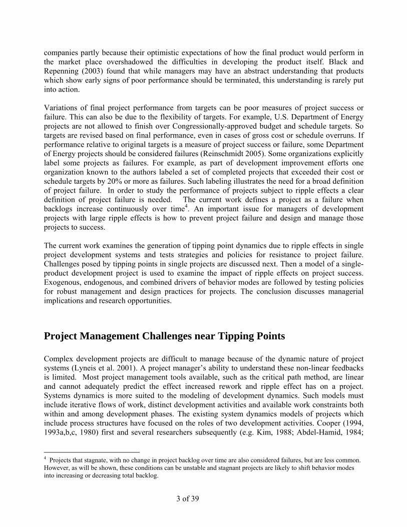
Figure 2: Workflow for a single project system (based on Ford and Sterman, 1998) A unique expansion of this basic model in the current work is the explicit modeling of ripple effects. As previously mentioned, ripple effects add work to a project beyond the original scope. Ripple effects are not iterative work, often generated from reinforcing loops within the project, to correct portions of the original scope. Ripple effects are work required in addition to completing and reworking the original project scope. This means that in order to simulate the effect of ripple effects, the basic workflow model shown in Figure 2 must be modified to allow additional work tasks to be added to the rework backlog during the course of a project. To model the ripple effect it is assumed when work is discovered to require rework that a proportional amount of additional work is added to the RW backlog: 5 Development activity flows represent the completion of a development task. Therefore backlogs, as used here, include work in progress.

6 of 39

REF = (DRW) (RES) (1) Where: REF - Ripple Effect {work packages / week} DRW - Discover Rework Rate {work packages / week}

RES - Ripple Effect Strength {dimensionless} The ripple effect strength is a project characteristic that describes the amount of impact that reworked portion of the project have on the total scope. The closed flow structure of the rework cycle allows for ripple effects to generate additional ripple effects when they are found to require rework. Equations (A.1) – (A.10) in Appendix A specify the stock and flow structure in Figure 2. Flows between the stocks of IC backlog, QA backlog, and RW backlog can be constrained by either the process rate or available resources (equations (A.11) – (A.16)). The process rate assumes infinite resources and is the amount of work that is available divided by the minimum amount of time required to perform a work package. The resource rate is the product of the number of resources assigned to each activity and the productivity of each resource. A resource allocation policy based on the bounded rationality of managers and simple heuristics is adopted here. In the basic model structure resources are allocated among the initial completion, quality assurance, and rework activities proportionally based on the current demand for each of these activities. The desired resource demand fraction for each activity is defined by the relative sizes of the backlogs (see Joglekar and Ford 2005 for more detail). For example, if productivities are equal and the current RW backlog is 40% of the current project backlog (ICbacklog+QAbacklog+RWbacklog) the rework activity would receive 40% of the available resources. Applied resource fractions are delayed with a first order exponential adjustment toward the desired fractions. This delay represents readjustment delays of the resource to the new assignment. Resource adjustment delays can be large due to the number of information and physical activities that must occur for a complete change in allocation, the time requirements for those activities, and the prerequisite information needs in those processes. For example, reallocating ironworkers from correcting flawed structural steel connections to inspecting new connections requires observing and collecting backlog sizes and current workforce allocations, forecasting demands for iron workers, determining desired allocations, informing the supervisor of the new targets, selecting and instructing the affected ironworkers, relocation of ironworkers and necessary equipment and tools, and the ramp-up of iron workers to full productivity in their new assignments. See Lee, Ford, and Joglekar (2005) for a study of the impacts of resource adjustment times on project performance. Model Validation and Typical Behavior The structure of the model was validated using standard methods for system dynamics models (Sterman, 2000). Basing the model on previously validated project models and the literature improves the model’s structural similarity to development processes and practices, as do unit consistency tests. Extreme condition tests were performed by setting model inputs, such as initial scope or total project staff to zero and simulating project behavior. As expected, no work was

7 of 39

performed. The model’s behavior for typical conditions is consistent with previous project models and practice (e.g. the "S" shaped growth of work released). Model behavior was also compared to actual project behavior as described by Ford and Sterman (1998 and 2003b) and Lyneis et al. (2001) and found to closely match the behavior modes of actual projects. Based on these tests the model was assessed to be useful for investigating tipping point dynamics in single development projects. Figure 3 shows typical project behavior for the total project backlog. As a successful project progresses the total backlog (IC, QA, and RW) initially decreases slowly as the value chain fills with work, increases progress during stable production and decreases to zero slowly as backlogs empty, indicating that the project is complete.

0

20

40

60

80

100

120

0 10 20 30 4Weeks

Tota

l Bac

klog

(Wor

k Pa

ckag

e

0

sTo

tal B

ackl

og (W

ork

Pack

ages

)

Figure 3: Typical project model behavior

Similar to Repenning (2001), project evolution is described with the project backlog as a fraction of the initial scope. Figure 4 shows the progression of the project backlog as a fraction of initial scope over time for three projects. The horizontal axis shows project backlog in the last time step and the vertical axis shows project backlog in the current time step. As an example of reading project behavior from the graph, the dashed lines show that in one of the projects the project backlog was 80% of the scope in the previous time period and 72% in the current time period. All projects begin in the center of Figure 4, with their backlog equal to their scope. Improving projects are reflected by conditions below the diagonal line, when preceding project backlogs exceed the current project backlog, and have a decreasing backlog. In contrast, degrading projects are reflected by conditions above the diagonal line (when current project backlogs exceed previous project backlogs) and theoretically have an ever-increasing unstable backlog. Successful projects end very near the origin6, when there is no more work backlog. Failed projects are reflected by continuously increasing backlogs in upper right corner of the graph. A project that remains on any point along the diagonal line has a constant project backlog and is considered to be stagnant. In the current model these conditions are not stable and projects tend to improve or degrade away from the diagonal.

6 The project simulation can reach the origin, when (BLt-1 , BLt) = (0,0), but actual projects stop when the backlog first reaches zero, when (BLt-1 , BLt) = (0,x) and x>0. This is represented in Figure 4 by a point on the horizontal axis very close to the origin.

8 of 39

0

0.2

0.4

0.6

0.8

1

1.2

1.4

1.6

1.8

2

0 0.2 0.4 0.6 0.8 1 1.2 1.4 1.6 1.8 2Total Backlog as a Fraction of Initial Scope (t-1)

Tota

l Bac

klog

as

a Fr

atio

n of

Initi

al S

cope

(t)

Beginning of Project

Degrading Project

Improving Project

Stagnation Line

Figure 4: Evolution of three projects near a project tipping point

Based on the previous discussions, projects with continuously increasing total backlogs are considered failures. These projects would be eventually terminated due to cost or schedule overruns. An upper limit describing project failure has been arbitrarily set at 2, when work remaining to be completed is twice the original scope. All simulations in the current work reaching this limit have continuously increasing total backlog. However, this limit may need to be adjusted for some projects. A Tipping Point Structure The feedback structure of the model is simple enough to be analyzed manually. Ford’s (1999) method for the analysis of loop dominance was applied. See Appendix B for detailed results and are summarized next. Figure 5 shows the reinforcing and balancing loops that drive the project.

9 of 39

Quality AssuranceBacklog

DiscoverRework Rate

Ripple Effect

Rework Backlog

+

+ R1

Approve WorkRate

QualityAssurance Rate

+

+

-

B1

frac discovered torequire rework

+Ripple EffectStrength

+

+

Rework Rate+

+

Work Released

+

Feedback Loop Legend

B1: Work Approval and Release Loop R1: Ripple Effect Loop Figure 5: Feedback structure controlling basic tipping point dynamics7

The Work Approval and Release loop (B1) is a balancing loop that withdraws work from the rework cycle. As the QA backlog increases from initial completion and rework the QA rate increases as resources are shifted to quality assurance (with a delay in resource allocation). Increasing QA increases the rate at which work is approved and removed from the QA backlog and added to the Work Released stock. Increasing the Approve Work rate decreases the QA backlog. This balancing loop drives the project to completion as the QA (and other) backlogs that represent the remaining project work decline to zero. In the absence of ripple effects loop B1 improves a project as quickly as process and resources allow. The Ripple Effect loop (R1) is a reinforcing loop that adds work to the project. Like in loop B1 increasing QA backlog increases the QA rate. In loop R1 this increases the rate at which work is discovered to require rework. As the Discover Rework rate increases the Ripple Effect increases, adding work to the RW backlog. The amount of ripple effect is driven by the ripple effect strength, which is the ratio of the amount of ripple effect work added to the RW backlog for each piece of work discovered to require rework. As the Rework Backlog increases resources are shifted to Rework (with a delay in resource allocation) and the Rework Rate increases. This adds more tasks to the QA Backlog, thereby increasing the Discover Rework rate further. In the absence of loop B1 (e.g. if the rework faction = 100%) loop R1 increases the rework and project backlogs infinitely, thereby degrading project performance to eventual failure. In many projects both loops B1 and R1 are active. In the improving project shown in Figure 4 the release loop (B1) is dominant and more work is being approved and removed from the rework cycle than is being added by ripple effects through loop R1. For the degrading project the ripple effect loop (R1) is dominant and more work is being added to the rework cycle than is being approved and released through loop B1. For stagnant projects (e.g. at the center of Figure 3) loops 7 Although not shown in the diagram a link exists between the “Discover Rework Rate” and the “Rework Backlog.” However, this link does not control exponential growth or decay and is not shown for simplicity.

10 of 39

B1 and R1 are balanced; work is being removed from the rework cycle at a rate equal to the rate at which work is added to the rework cycle. The relationship described by the two feedback loops in Figure 5 can be described using a tipping point. Project Tipping Point Conditions The tipping point is the conditions where a project ceases showing improvement and begins to degrade, or vice versa. Using the model equations from the work flow sector we describe the tipping point conditions and conditions for project improvement or degradation. The tipping point is where the work approved and released rate (RA), is equal to the ripple effect rate (REF). The rate at which work is approved and released is the compliment of the QA rate (RQA) that is discovered to require rework (DRW). Therefore, at the tipping point:

REF = RA = RQA – DRW (2) Where:

REF ripple effect {work packages/week} RA approve and release work rate {work packages/week} RQA quality assurance rate {work packages/week} DRW discover rework rate {work packages/week}

From the work flow model equations (Appendix A) Ripple Effect (REF) is the product of the discover rework rate (DRW) and the Ripple Effect Strength (RES) and the rate at which rework is discovered (DRW) is the product the QA rate (RQA) and the rework fraction (FRW). Equation (2) then becomes: (RES)(RQA)(FRW) = RQA – (RQA)(FRW) (3) simplification yields a description of the threshold conditions that define the tipping point.

FRW (RES + 1) = 1 (4) When the left hand side of equation (4) exceeds 1 the project is degrading, when less than 1 the project is improving, and when equal to 1 the project is stagnate. The tipping point conditions are shown graphically in Figure 6.

11 of 39

0.0

0.1

0.2

0.3

0.4

0.5

0.6

0.7

0.8

0.9

1.0

0 2 4 6 8

Ripple Effect Strength (R ES )

Frac

requ

iring

rew

ork

(F rw

)

10

F RW = 1/(R ES + 1)

Project Degrades

Project Improves Unstable Equilibrium

Figure 6: Basic project tipping point conditions Figure 6 can be used to intuitively explain the behavior of projects near the tipping point. The total backlog of projects to the lower left of the solid line decrease and the project improves. The total backlog of projects to the right of the solid line increase and the project degrades. The solid line represents possible tipping point conditions. A project can only remain at a tipping point if the loop B1 completes work at exactly the rate as loop R1 adds work to the project backlog (Eq. 2). In the absence of forces to keep the project stagnate, small digressions from the tipping point conditions in either direction will cause the project to improve or degrade. If either loop dominates total backlogs will increase (R1 dominates) to project failure or decrease (B1 dominates) to project completion. Therefore the tipping point is an unstable equilibrium. Project conditions that move across the tipping point conditions shown in Figure 6 experience a change in project behavior mode from increasing to decreasing or vice versa. The shape of Figure 6 reveals intuitive insights about project conditions that generate tipping point dynamics. The negative slope of the tipping point conditions line indicates that projects that have low ripple effect strength (RES) can tolerate a higher fraction of rework (FRW) before degrading and projects with low rework fractions (FRW) can tolerate higher ripple effect strengths. However, the tipping point relationship between ripple effect strength and rework fraction is not linear. A small increase in a small ripple effect strength greatly reduces the tolerable rework fraction. But as ripple effect strength increases the tolerable rework fraction decreases more slowly, asymptotically toward a value of zero.

12 of 39

Figure 6 can help explain how projects can be overwhelmed by rework and ripple effects. Consider the fate of some nuclear power plant construction projects in the United States8. The first commercial nuclear plant to come on-line in the United States was Dresden 1, located in Illinois, in 1959 (NRC 1982). Between 1959 – 1969 twelve nuclear plants were completed with an average construction duration of 46 months (NRC 1982). Between 1970 – 1981 the average duration nearly tripled, reaching 131 months in 1981 (NRC 1982). While the plants constructed during this time were higher capacity units (i.e. bigger) than earlier projects, most researchers identify the ever increasing (and ever changing) number of governmental regulations imposed on nuclear plants as the root cause for cost and duration increases in nuclear plant construction (Lake 2002, Kharbanda and Pinto 1996, Feldman et al. 1988, and Lillington 2004, Friedrich et al. 1987). A specific example of the effect of changing governmental regulation in nuclear plant construction is the changing requirements for pipe supports. In 1971, a new regulation was adopted that required all pipes within a nuclear power plant to be supported (Aron 1997). This included pipes within the reactor containment building (the large concrete dome seen at all U.S. nuclear plants). Designers failed to take into account the effect this change would have on plant design. One such example is the Shoreham plant in Long Island, New York. Figure 7 shows the progress of construction of the Shoreham plant. Construction began in 1972 and was to be completed in the first quarter of 1977. In September of 1977 the expected duration was increased by over 12 months due to material shortages, labor productivity, and “design changes due to regulatory requirements” (NRC 1982). The original estimate of $217 million was well short of the actual $5 billion cost when the plant was completed (Aron, 1997). Construction activities were completed in the mid 1980’s but the plant never came on-line due to political pressure over concerns of evacuating Long Island in the event of an accident (Aron, 1997) Although the plant did not begin construction until 1972, the design was already completed and approved before the new pipe support regulations took effect. According to a former Vice-President of the architect/engineering/construction firm building the Shoreham plant, during construction, the pipe supports had to be designed and installed (Reinschmidt 2005). As these supports were outside the initial scope they provide an example of ripple effect.

8 Sterman (2000, pp. 423-4) models a similar experience based upon plant construction times to illustrate the impacts of average durations in an aging chain and Little’s Law.

13 of 39

0%

10%

20%

30%

40%

50%

60%

70%

80%

90%

100%

Jul-72 Dec-73 Apr-75 Aug-76 Jan-78 May-79 Oct-80 Feb-82 Jul-83

% C

ompl

ete

% C

ompl

ete

Figure 7: Shoreham Construction Progression 1973-1982 (Data from NRC)

Ripple effect problems were not limited to the Shoreham plant. Friedrich et al. (1987) referred to the “reengineering and redesign” of pipe supports as a “frequently encountered event” in nuclear plant construction. Changing regulations along with changes in market conditions helped the economic viability of nuclear plants become suspect. A 1988 study (Feldman et al.) suggested that for most nuclear power plants under construction in the United States at the time, it would be more economical to either cancel the plants under construction, regardless of progress, or modify the plants to burn conventional fuel (coal, gas, or oil). This illustrates the large impacts that ripple effects can have on major development projects. Project Trajectory Reversal and Schedule Pressure We next investigate projects that begin on one side of the tipping point but, due to endogenous or exogenous influences, are pushed past the tipping point and reverse their behavior mode from improving to degrading or visa versa. As used here, project trajectory reversal is when the status of a project initially improves but later degrades and eventually fails (i.e. when an improving, “good,” project degrades, “goes bad”) or vice versa. Project trajectories that are monotonically improving or monotonically degrading (e.g. Figure 4) do not describe trajectory reversal. However, our study of large complex construction projects such as nuclear power plants indicate that trajectory reversal is an important issue. If project resources and productivity are limited and fixed, the basic project tipping point structure described above cannot endogenously simulate projects with trajectory reversal. This is because the structure lacks a mechanism to shift feedback loop dominance from

14 of 39

loop B1 to R1 in Figure 5. Exogenous influences, additional endogenous dynamic structures, or both, are required to propel projects beyond the tipping point and reverse their trajectory9. Exogenous Influences on Tipping Point Dynamics Exogenous factors can influence the rework fraction or ripple effect strength, such as changes in project scope during construction or, as with the case of the nuclear plant, changes in requirements. An inspection of equation (4) shows that, if a project starts far enough away from its tipping point (e.g. FRW (RES+1) <<1) and the increases in the rework fraction and ripple effect strength are small enough, that the project does not cross the tipping point and behaves essentially like a monotonically improving project. However, if the magnitude of the changes is large enough the project could be pushed past the tipping point, causing a project that initially improved to reverse its trajectory and degrade. However, as will be demonstrated next, pushing a project beyond its tipping point is not always sufficient to trap the project there and cause project failure. Figure 6 shows the behavior of a project that begins with FRW = 0.2 and RES = 1. Applying equation (4) (FRW (RES+1) =0.2(1+1) =0.4<1) places the project on the improving side of the tipping point (pt. 1 in Figure 6). The project progresses towards completion until, at week 10 the rework fraction was exogenously raised to 0.6 to reflect a new but temporary problem that the development team must address. The tipping point conditions jump to 1.2, pushing the project quickly past the tipping point (pt. 2 in Figure 8). The project degrades and the project backlog increases. The project continues to degrade until the rework fraction is exogenously returned to the original condition and the tipping point conditions return to their original level (pt. 3 in Figure 8). Once the project is operating below the tipping point again it begins to reduce the project backlog (pt. 4 in Figure 8), thus improving to completion (pt. 5 in Figure 8). This demonstrates how improving projects subjected to large but temporary exogenous increases in the rework fraction, ripple effect strength, or both can be pushed beyond their tipping point and begin to degrade. But, barring structures that prevent a full and immediate recovery of those factors, when the exogenous change is removed the project crosses the tipping point again and can improve again.

9 Delays that can also cause shifts in feedback loop dominance by temporarily constraining a strong loop are not addressed here.

15 of 39

0

0.2

0.4

0.6

0.8

1

1.2

1.4

1.6

1.8

2

0 0.2 0.4 0.6 0.8 1 1.2 1.4 1.6 1.8 2

Total Backlog as a Fraction of Intial Scope (t-1)

Tota

l Bac

klog

as

a Fr

atio

n of

Initi

al S

cope

(t)

1) Project begins below the tipping point

2) Temporary problem increases base rework fraction and pushes the project above the tipping point.

3) The temporary problem is solved and the base rework fraction returns to the original fraction.

5) Project C l t

4) Since the base rework is returned to its original fraction the project remains the same distance from the tipping point as before.

Tota

l Bac

klog

as

a Fr

actio

n of

Intia

l Sco

pe (t

)

Figure 8: Project exogenously pushed beyond the tipping point

As modeled above a sustained exogenous impact or another dynamic structure is required to cause an improving project to both reverse its trajectory and fail. In contrast to the behavior in the example above and in Figure 8, permanent exogenous changes in the rework fraction, ripple effect strength, or both that keep the project conditions beyond the tipping point (i.e. FRW(RES+1)>1) generate project failure. Simulations not shown here for brevity verify these results. A side effect of the temporary problem in the example above is that the project will have a longer duration than it would have if the rework fraction had not increased. The time projects spend beyond the tipping point increases the total required work. If resource quantities and productivity is limited, this can cause projects to be completed far later than without the trajectory reversal. But, given enough time, the project will finish. This may be a partial explanation of projects that are very difficult to terminate and have very poor schedule performance such as the Department of Energy projects described previously. In other cases economic or other types of deadlines may cause these projects to be terminated, such as with nuclear plants that were never completed (Nuclear Engineering International 1995). Endogenously Influenced Tipping Point Project Failure Some projects reverse their trajectory from improving to degrading and fail with continuously increasing project backlogs due to temporary problems. This suggests that temporary problems influence projects after the problem is resolved in ways that can cause failure. Schedule pressure is a common side effect of temporary development problems that can have important impacts on

16 of 39

performance. Schedule pressure is the effect an approaching project deadline has on project participants. As a project approaches a rigid deadline, work pace is increased to meet the deadline, thus the schedule pressure increases the risk of work being completed incorrectly. Schedule pressure increases as expected completion dates extend beyond required deadlines and can lower development quality and increase rework (Cooper 1994, Graham 2000, Ford and Sterman 2003b). We introduce schedule pressure into the model to investigate the potential for interactions between schedule pressure and tipping point structures to induce project failure. In our model schedule pressure (Figure 9) is modeled similar to the structure developed by Ford (1995), in which the schedule pressure ratio increases with the time required to complete the remaining work and decreases with the time available to complete that work. The time required (TR) is modeled based on the project backlog and the average productivity of releasing work. The time available (TA) is the difference between the deadline and the current time. To explicitly model the impacts of schedule pressure on tipping point dynamics we disaggregate the rework fraction into two components: the minimum rework fraction (mFRW) and the variable rework fraction (vFRW). The minimum rework fraction is the fraction requiring change that reflects basic project complexity. The variable rework fraction is the additional fraction of work requiring change due to schedule pressure and other factors. Increases in the variable rework fraction reflect more mistakes made by developers due to the pressure to meet the project deadline. The variable rework fraction is modeled as the product of a reference fraction (assumed to be 1) and the impact of schedule pressure. Schedule pressure impact is modeled as the schedule pressure ratio (shifted from a no-pressure value of 1 to 0) and the sensitivity of the rework fraction to schedule pressure (SRW-S). Therefore:

FRW = mFRW + vFRW = mFRW + [((TR / TA)-1) (SRW-S) (vFRW′)] (5)

Where:

mFRW - minimum rework fraction {percent} vFRW - variable rework fraction {percent} TR - time required to complete backlog {weeks} TA - time available to complete backlog {weeks} SRW-S - sensitivity of rework fraction to schedule pressure {percent} vFRW′ - reference of base variable rework {percent}

Figure 9 shows the tipping point structure in Figure 5 with schedule pressure. Loop (R2) can increase the strength of the ripple effect loop (R1) by increasing the rework fraction as described above. As the project (total) backlog increases the Time Required to complete the project increases, increasing Schedule Pressure. This increases the variable rework fraction, Fraction Discovered to Require Rework, and thereby the Discover Rework Rate. This increases the Ripple Effect which adds work to Rework Backlog, which increases the Project Backlog10. As will be shown, this simple schedule pressure structure can drive a project over the tipping point without exogenous

10 A third reinforcing loop exists that in which the RW backlog and Rework increase the QA Backlog, which also increases the Project Backlog. This loop performs like the R2 loop but instead of increasing the Total Backlog through Rework, it is increased through the QA Backlog.

17 of 39

influences or trap a project beyond the tipping point that would otherwise revert to an improving behavior mode and be completed.

Quality AssuranceBacklog

DiscoverRework Rate

Ripple Effect

Rework Backlog

+

+ R1

Approve Work RateQA Rate+

+

-

B1

Frac Discovered toRequire Rework

+Ripple EffectStrength

+

+

Rework Rate+

+

Work Released

+

Total Backlog+

+

Initial CompletionBacklog

+

Time Required

+

Schedule Pressure+

Project Deadline

-

R2

Variable ReworkFraction +

+

Feedback Loop Legend

B1: Work Approval and Release Loop R1: Ripple Effect Loop R2: Schedule Pressure Loop

Figure 9: Reinforcing feedback between schedule pressure and rework Setting aggressive deadlines is common in development projects. This generates schedule pressure, which can cause performance problems in development projects (Lyneis et al. 2001, Ford and Sterman 2003a). Here we investigate the impacts of schedule pressure due to aggressive deadlines on project performance through ripple effects. Figure 10 shows the behavior of two projects (A and B) with different deadlines and therefore different amounts of schedule pressure. Without schedule pressure (feedback loop R2 inactive) the two projects finish in 25 weeks. The expected duration for project A has been reduced by 20% (20 weeks instead of 25 weeks). Project B has had its expected duration reduced by 28% (18 weeks). The interaction of schedule pressure and the tipping point have a dramatic impact on project performance. Project A remains on the improving side of the tipping point and finishes, but schedule pressure pushes Project B past the tipping point, causes trajectory reversal, and leads to failure. Simulations verify that the amount of schedule pressure that can be absorbed without trajectory reversal is related to the distance the project starts away from its tipping point conditions. These simulations demonstrate that projects can absorb safely some schedule pressure, but that in the presence of a tipping point structure too much schedule pressure can cause projects to fail. The ripple effect–schedule pressure reinforcing loop provides an endogenous explanation for how projects that begin in conditions that can lead to success can become trapped beyond the tipping point, degrade, and fail.

18 of 39

0

0.2

0.4

0.6

0.8

1

1.2

1.4

1.6

1.8

2

0 0.2 0.4 0.6 0.8 1 1.2 1.4 1.6 1.8 2

Total Backlog as a Fraction of Initial Scope (t-1)

Tota

l Bac

klog

as

a fr

actio

n of

initi

al s

cope

(t)

Projects begins below the tipping point.

Project B: Expected project duration of 28% pushes the project over the tipping point and leads to failure.

Project A: 20% decrease in expected project duration still alows the project to finish.

Tota

l Bac

klog

as

a Fr

actio

n of

Intia

l Sco

pe (t

)

Figure 10: Effect of schedule pressure on project performance mode

Compound Project Failure Most development projects experience temporary problems and many have aggressive deadlines. In these cases, as shown above, development projects can be doomed or likely to fail due to a tipping point structure. However, projects that can succeed despite temporary problems but do not are of particular interest to development project managers because they provide opportunities for improvement. The model and tipping point structure shown in Figure 9 illuminates these circumstances. Schedule pressure can trap projects that would, under normal circumstances finish, beyond the tipping point and drive them to failure. Figure 11 describes such a project. When applied individually a temporary problem (Figure 8) or moderate schedule pressure (Project A in Figure 10) do not initiate permanent project degradation to failure. However, their combined impacted is enough to permanently push the project past the tipping point.

19 of 39

0

0.2

0.4

0.6

0.8

1

1.2

1.4

1.6

1.8

2

0 0.2 0.4 0.6 0.8 1 1.2 1.4 1.6 1.8 2

Total Backlog/Initial Scope (t-1)

Tota

l Bac

klog

/Initi

al S

cope

(t)

1) Project begins below the tipping point.


3) The temporary problem is solved and the base rework fraction returns to the original fraction but shedule pressure has moved the project closer to the tipping point.

4) The schedule pressure continues to increase and finally pushes the project past the tipping point to failure.

Tota

l Bac

klog

as

a Fr

actio

n of

Intia

l Sco

pe (t

)

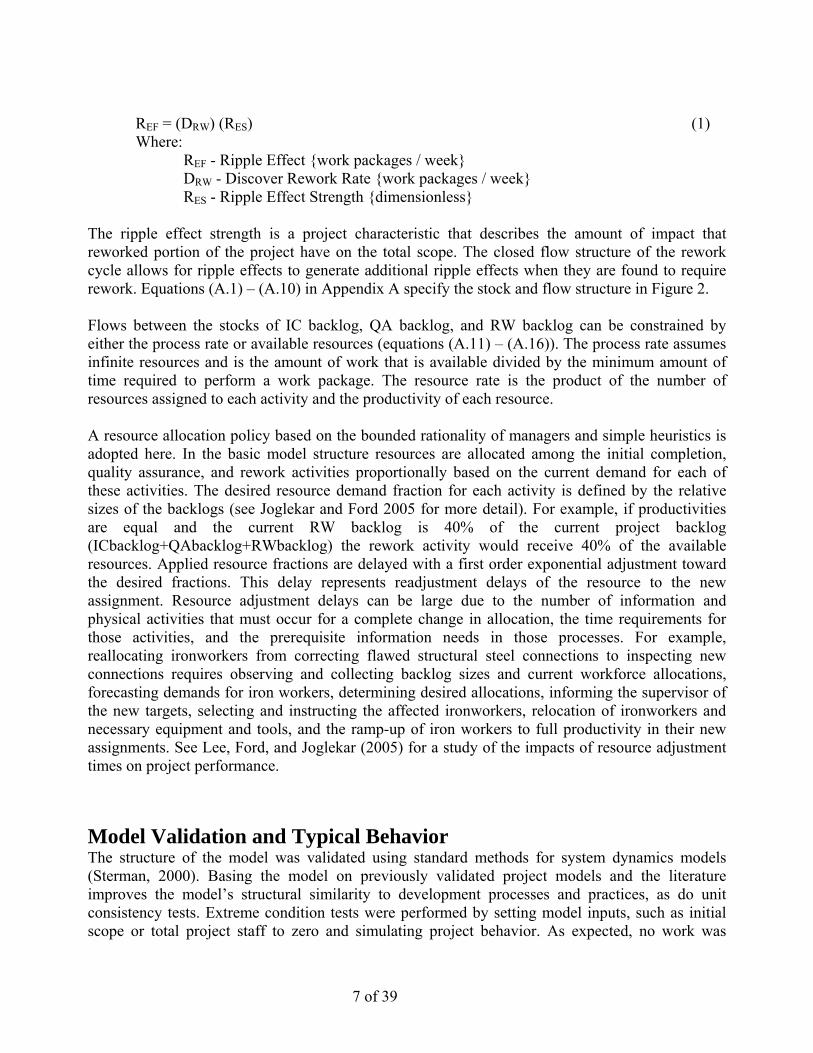
Figure 11: Interactive impact of a temporary problem and schedule pressure on a project

Consider a development project with an aggressive deadline that experiences an unexpected problem that temporarily increases the rework fraction. The project (see Figure 11) begins below the tipping point (pt. 1) and improves. In week 10 an exogenous temporary problem is encountered that pushes the project over the tipping point (pt. 2). The project begins to build project backlog, degrade, and increase schedule pressure. When the problem is resolved and the temporary increase in the rework fraction is removed the project dips below the tipping point and begins to improve again (pt.3), but remains closer to the tipping point line than its previous position. This is due to the increased project backlog generated by the temporary problem increasing the schedule pressure and therefore the rework fraction and ripple effect. In contrast to the project without schedule pressure, the rework fraction increases after the temporary problem is resolved due to the higher schedule pressure. This activates loop R2, increasing the ripple effect, project backlog, and schedule pressure. Eventually project conditions exceed the tipping point again (pt. 4) and the project crosses the tipping point a second time, this time due to endogenous causes. We have demonstrated several scenarios in which an improving (“good”) project can experience trajectory reversal and degrade to failure (“go bad”). Schedule pressure, an endogenous influence, can also push a project to failure. The experience shown in Figure 11 reflects a common problem that can be generated by a simple feedback structure (Figure 9). In the next section we use this problem as the basis for testing strategies for managing development projects near a tipping point to avoid project failure or save projects that are degrading.

20 of 39

Project Management near a Tipping Point Strategies for managing projects near a tipping point include avoiding tipping points, resource management, backlog management, and schedule management.

Avoiding Tipping Points Avoiding tipping point conditions such as those described above entails the selection or design of development projects with relatively low rework fractions and ripple effects. Project selection may include an assessment of project complexity and interdependence and their impacts on the probability of success. Some projects or portions of projects may have characteristics that allow this strategy. For example, construction projects often use relatively simple technologies and processes to constrain rework fractions and project planning purposefully keeps these operations separate to constrain ripple effects. Even projects with inherently high rework fractions and ripple effects can be designed to apply this strategy through methods such as modular design (Baldwin and Clark 2000). Modular design develops projects as sub-systems that can be adjusted independently with minimal impact on the design as a whole. By designing projects with loose dependencies, if a design change does arise, it can be corrected with minimal impact on other systems. Figure 6 helps illustrate how a modular project with relatively low ripple effect strength would be able to tolerate a higher rework fraction without crossing the tipping point (i.e. it would reside in the lower left of the chart). In the model, modular designed projects would have a lower ripple effect strength and would therefore be insulted from additional work added by the ripple effect. Modular design allows complex projects (with high rework fractions) to progress because a reduction in ripple effects has been designed into the project. An example of modular design from the automotive industry is Toyota’s method for designing components of a new car model. During the design of a new model Toyota will provide their brake system supplier with specifications regarding the weight of the car, the desired stopping distance from a given speed, and how much space the brake system can occupy in the wheel assembly (Womack et al. 1991). The brake supplier can change the design of the brake system without impacting other project components as long as the required specifications are met. Although technology selection, project planning, and modular design are helpful tools they often cannot completely eliminate ripple effects from projects. Resource Management Resource management includes altering the quantities of resources, their productivities, altering resource priorities to meet resource demands, anticipating future resource demands, and adjusting resources from current to needed applications. One reasonable response to a project that has crossed the tipping point is to add more resources to the project. The justification would be that since a project has more work, more resources are needed to complete the work. Model simulations show that increasing a project’s resource level when a project crosses the tipping point can “save” the project, but this must be approached carefully. If adding resources does not reduce the rework fraction adequately through increased expertise (for example) reduced schedule pressure, or other factors, the tipping point dynamics remain effectively the same. This can often be the case. Brooks (1982) states that, “adding manpower to a late software project makes it later.” Likewise, if

21 of 39

inexperienced resources are added to a project, particularly one that is complex, the amount of discovered rework could increase (Graham 2000, Lyneis et al. 2001). In these cases adding resources to a project that has begun to degrade would increase the rate of degradation. More resources making more mistakes would drive the project beyond the tipping point faster than fewer resources. Therefore managers must be careful when adding resources to a project near tipping points. Often the preceding strategy is unavailable because resource quantities for development projects are limited or fixed. A second strategy is to allocate resources to maximize the flows of work through the project. Certain backlogs could be given priority to resources based upon a manager’s understanding of the critical aspects of the system. Black and Repenning, (2001) studied this policy in multi-project systems. Repenning (2001) argues that “creating ‘fire-resistant [tipping point resistant]’ [new product development] systems requires the development of more dynamic methods of resource planning.” He suggests that this planning method use the present state of the system to forecast the future resource needs. The basic model as described above follows this recommendation. In the basic model managers are assumed to allocate the same fraction of resources to each activity as the activity’s current backlog contributes to the project backlog. A simple and reasonable extension of this policy is to assume that managers base allocations on their forecasts of resource needs at a time in the future. This is consistent with Cooper’s (1994) suggestion that “developing an information system to forecast resources committed to known projects as well as resource availability as a function of time is no easy task, but it is essential.” Thomke and Fujimoto (2000) suggest shifting resources to earlier parts of projects as the key to success, stating “faster product development can be achieved with an earlier generation of problem-and solution related information, particularly if it involves critical path activities.” Joglekar and Ford (2005) use a control theory model and system dynamics to evaluate the impacts of forecasting resource demand on project schedule performance. Sterman’s (2000, p. 634-6) structure for modeling trends is adopted11 and the resulting trend linearly extrapolated from current backlog sizes into the future the time required to reallocate resources. Sterman describes and explains the model structure and the equations that govern the resource forecasting system are included in Appendix C. Resource Management Impacts on a Degrading Project We simulated the potentially-successful project that became trapped beyond the tipping point and failed (Figure 11) across a range of resource adjustment times and demand forecasting policies from no forecasting to forecasting with long time horizons. As shown in Figure 12 resource forecasting can save the project. The project begins below the tipping point (pt. 1). At some point a temporary problem is encountered that pushed the project past the tipping point (pt. 2). Once this problem is resolved, the project returns below the tipping point. Schedule pressure pushes the project close to the tipping point (pt. 4) after the project recovers from the temporary problem. As RW and QA backlogs begin to increase, resources are shifted far enough in advance and fast enough to prevent the backlogs (through schedule pressure) from pushing a project across the

11 The exception to the use of Sterman’s trend structure is that only two exponential smoothing loops (rather than three) are used. Sterman’s structure uses the third exponential loop to smooth “noisy” data fed into the structure. The input data to our structure is already smooth so this third loop is unnecessary.

22 of 39

tipping point. A policy that uses four weeks of backlog history to develop a trend that is projected four weeks into the future can save the project if adjusted quickly enough (≤ 4 weeks).

0

0.2

0.4

0.6

0.8

1

1.2

1.4

1.6

1.8

2

0 0.2 0.4 0.6 0.8 1 1.2 1.4 1.6 1.8 2


Tota

l Bac

klog

/Initi

al S

cope

(t)

1) Project begins below the tipping point.



4) Resources are adjusted to prevent the build up of backlog from increasing the schedule pressure to a point that would push the project past the tipping point.

5) Project Complete

Tota

l Bac

klog

as

a Fr

actio

n of

Intia

l Sco

pe (t

)

Figure 12: Use of resource forecasting to save project

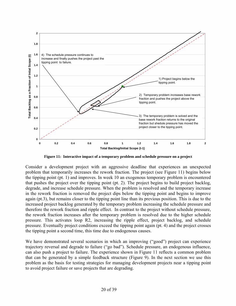
Initial results show that longer trend adjustment times (i.e. a slow reacting manager) prevent the trend from reacting quickly enough to the increases in backlogs to allow resources to be allocated fast enough to save the project. Shorter trend adjustments (i.e. a quick reacting manager) pull the project farther away from the tipping point. This suggests that managers should react quickly to changes in project work backlogs. Resource Adjustment Times The time required to shift resources across development activities also impacts performance. Lee, Ford, and Joglekar (2004) found that resource adjustment times can have important impacts on project schedule performance. Their model simulations identified that there exists optimal resource adjustment times that minimize project duration over a range of project complexities. Reducing resource adjustment times while still utilizing proportional resource allocation policies can also save the project. Figure 13 shows the problem project (Figure 11) with a resource adjustment time reduced from 4 weeks to 3 weeks. Faster adjustments of resources towards target levels cause the schedule pressure to decrease after the removal of the temporary problem ( Figure 13 pt. 4) and saves the project from continuous degradation (Figure 11).

23 of 39

0

0.2

0.4

0.6

0.8

1

1.2

1.4

1.6

1.8

2

0 0.2 0.4 0.6 0.8 1 1.2 1.4 1.6 1.8 2

Total Backlog as a fraction of initial scope (t-1)

Bac

klog

as

a fr

actio

n of

initi

al s

cope

(t)

1 ) Project begins below the tipping point.



5) Project Complete

4) Schedule pressure has pushed the project closer to the tipping point but it is not strong enough to drive the project to failure.

Tota

l Bac

klog

as

a Fr

actio

n of

Intia

l Sco

pe (t

)

Figure 13: Use of decreased resource adjustment time to save project

Both resource forecasting and reduced staff adjustment times provide managers levers that can be used to save failing projects. Forecasting resources is somewhat straight forward provided a manager can make a reasonable estimate of expected future work. From the authors own experience the success of this policy is highly dependant on the accuracy of the estimate. One must also ensure that a change in the projected trend is reflective of changing resource requirements. Reducing staff adjustment times can be more challenging than resource forecasting but appear to have a greater impact. Backlog Management Backlog management involves canceling work or releasing defective work. Work cancellation is a reduction during the project of features or scope of a project. Model simulations (not shown here for brevity) show that, if enough work is canceled, that canceling defective work can prevent a project from being overwhelmed with rework. As expected, projects nearer the tipping point required the cancellation of more work than those farther away. Black and Repenning (2001) found similar results using work cancellation in a multi-project system. Schedule Management One factor that controls schedule pressure is the project deadline. Both Cooper (1994) and Graham (2000) argue that setting realistic project deadlines reduces the amount of rework on a project.

24 of 39

Therefore, an important part of schedule management is monitoring the project deadline and ensuring that it is realistic. One way to ensure a realistic deadline is to implement a flexible deadline. A flexible deadline is dependent upon the amount of work left to be completed in a project. A rigid deadline does not take into account changes or delays in a project caused by rework and ripple effects. Flexible deadlines take these effects into account by adjusting the expected completion date based upon the time required to complete the total project backlog. To model this flexibility the project deadline moves toward the expected completion date at a rate based on the flexibility of the deadline and the difference between the expected completion data and deadline. The effectiveness of flexible deadlines in saving the problem project (Figure 11) was tested. Figure 14 shows how a flexible deadline prevents the increased backlog due to the temporary problem from increasing schedule pressure. This prevents schedule pressure from building up to a point that would drive the rework fraction high enough to push the project beyond the tipping point. This suggests that managers can use deadline flexibility to recover projects from degradation initiated by crossing a tipping point.

0

0.2

0.4

0.6

0.8

1

1.2

1.4

1.6

1.8

2

0 0.2 0.4 0.6 0.8 1 1.2 1.4 1.6 1.8 2


Bac

klog

as

a fr

actio

n of

initi

al s

cope

(t)

1 ) Project begins below the tipping point.



5) Project Complete

4) Schedule pressure has pushed the project closer to the tipping point but it is not strong enough to drive the project to failure.

Tota

l Bac

klog

as

a Fr

actio

n of

Intia

l Sco

pe (t

)

Figure 14: Use of flexible schedule on project past the tipping point

25 of 39

Conclusions Tipping point structures are integrated with single development project dynamics to examine project behavior modes. The tipping point is useful because it allows comparison of project failure due to different causes. Rework and ripple effects can combine to push projects to fail. By understanding these failure mechanisms potentially robust policies are examined that can decrease the risk of failure for projects near the tipping point threshold. Successful policies where those that avoided the tipping point by reducing rework and ripple effect or those that reduced backlogs by effectively managing resources. The policies tested provide several managerial implications. Tipping point conditions (Eq. (4)) support the use of modular design in the development of complex products. By reducing the ripple effect, modular design would allow more aggressive projects to be pursued with reduced risk of failure. As described in the discussion of Toyota’s brake system design, modular design allows concurrent development of project tasks with minimal interdependence. Project managers would benefit from preliminary designs which set project specifications to allowing concurrent modular design. Proper resource management can play an important role in project success. Resource forecasting with quick identification of changing trends has the potential to further insulate projects from the tipping point. Model simulations show that the most successful policies are those which are short in hindsight and forecast farther into the future. However, one limit of the model used here is that it benefits from data free of the “noise” typically associated with actual project tracking reports. Managers must be careful to ensure that a perceived project trend change is an actual change in project progression and not normal oscillations in project progress reporting before adjusting resources. Resource adjustment times were also found to be potentially effective in responding to projects vulnerable to tipping point dynamics. Quicker adjustment times for both proportional and forecasted resource allocation policies were beneficial in preventing projects subject to schedule pressure from crossing the tipping point. Again, the model is limited in that it does not take into account the negative effects (worker morale, lost production time, etc.) of shifting resources. Other work (Lee et al. 2004) has shown that there is an optimal adjustment time for resources, below which can be detrimental to a project. While flexible resources can be beneficial to a project, the key for managers is to ensure that resources are be adjusted in an efficient manner. Finally, realistic deadlines can help prevent a project from being overwhelmed with schedule pressure. Managers need to carefully consider how changes in work volume, through either increased rework or scope changes, affect a project’s deadline. Model simulations show that managers should resist the temptation to strive for schedules which have become unrealistic due to drastic changes in a project’s work volume. This is supported by other research (Lyneis et al. 2001 and Graham 2000). The model structure used in this work has several limitations. This includes the assumption that all work released is of one quality. This prevents a policy investigation similar to Black and Repenning (2001) of releasing lower quality work in a single project system. In addition the model does not take into account work that must be redone due to rework. Improved models that take into account

26 of 39

these conditions are needed to fully examine polices that govern single project development. Future research can improve model structure consistency with actual projects and calibrate the model to practice. Tipping point dynamics can strongly influence the behavior and performance of individual development projects, and sometimes determine their success or failure. Continued improvement in the understanding of tipping point dynamics can lead to better development project management and performance. Acknowledgement: The authors thank Prof. Nitin Joglekar for suggesting the positioning of this paper, Prof. Kenneth Reinchmidt for assisting in nuclear power plant investigation, and Marsha Ward, NRC Research Librarian, for assisting in the acquisition of NRC nuclear power plant construction data and three anonymous reviewers of a draft of this paper.

27 of 39

References Adbel-Hamid, T.K. 1984. The dynamics of software development project management: An integrative systems

dynamics perspective. Doctoral thesis, Massachusetts Institute of Technology. Cambridge, MA.

Abelson, P. 1996. Nuclear Power in East Asia. editorial, Science, Vol. 272: 465.

Aron, J. 1997. Licensed to Kill? The Nuclear Regulatory Commission and the Shoreham Power Plant. University of Pittsburgh Press: Pittsburgh, PA.

Baldwin, C. and Clark, C. 2000. Design Rules: The Power of Modularity. MIT Press. Cambridge, MA.

Black, L. and Repenning, N. 2001. Why firefighting is never enough: preserving high-quality product development. System Dynamics Review. 17(1): 33-62.

Brooks, F. 1982. The Mythical Man-Month. Addison-Wesley Publishing Company Inc., Philippines.

Cooper, K.G. 1980. Naval ship production: A claim settled and a framework built. Interfaces. 10(6): 20-36.

Cooper, K.G. 1993a. The rework cycle: why projects are mismanaged. PM network. February: 5-7.

Cooper, K.G. 1993b. The rework cycle: how it really works . . . and reworks. PM network. February: 25-28.

Cooper, K.G. 1993c. The rework cycle: benchmarks for the project managers. Project Management Journal 14(1): 17-21.

Copper, K.G. 1994. The $2,000 hour: How managers influence project performance through the rework cycle. Project Management Journal. 15(1): 11-24.

Courtney, H. and Lovallo, D. 2004. Brining rigor and reality to early-stage R&D decisions. Research·Technology Management. 47(5): 40-45.

Feldman, S., Bernstein, M., and Noland, R. 1988. The costs of completing unfinished US nuclear power plants. Energy Policy. 16(3): 270-279.

Ford, D. 1995. The Dynamics of Project Management: An Investigation of the Impacts of Project Process and Coordination on Performance. doctoral dissertation. Massachusetts Institute of Technology, Cambridge, MA. 1995.

Ford, D. and Sterman, J. 1998. Modeling Dynamic Development Processes. System Dynamics Review. 14(1): 31-68.

Ford, D. 1999. A behavioral approach to feedback loop dominance analysis. System Dynamics Review. 15(1): 3-36.

Ford, D. and Sterman, J. 2003a The Liar's Club: Impacts of Concealment in Concurrent Development Projects. Concurrent Engineering Research and Applications. 111(3): 211-219.

Ford, D. and Sterman, J. 2003b Overcoming the 90% Syndrome: Iteration Management in Concurrent Development Projects. Concurrent Engineering Research and Applications. 111(3): 177-186.

Friedrich, D., Daly, J., and Dick, W. 1987. Revisions, Repairs, and Rework on Large Projects. Journal of Construction Engineering and Management. 113(3): 488-500.

Joglekar, N. and Ford, D. 2005. Product Development Resource Allocation with Foresight. European Journal of Operational Research. 160(1): 72-87.

Kharbanda, O. and Pinto, J. 1996. What made Gertie Gallop: Learning from Project Failures. New York. Van Nostrand Reinhold.

Kim, D.H. 1988. Sun Microsystems, Sun3 product development/release model. Technical Report D-4113. Systems Dynamics Group, Sloan School of Management, Massachusetts Institute of Technology, Cambridge, MA.

Lake, J. 2002. The Fourth Generation of Nuclear Power. Progress in Nuclear Energy. 40(3-4): 301-307. Lee, N. 1995. Powering up of TVA reactor generates safety debate. The Washington Post: December 3, 1995. p.

A22-A-23.

28 of 39

Lee, Z, Ford, D. and Joglekar, N. 2004. The Design of Resource Allocation Policies Proceedings of the 2004 International System Dynamics Conference, Oxford, UK, July 25-29.

Lillington, J. 2004. The Future of Nuclear Power. Elsevier. United Kingdom. Lyneis, F. Cooper, K. Els, S. 2001. Strategic management of complex projects: a case study using system dynamics.

Systems Dynamics Review. 17(3): 237 – 260.

Matta, F. and Ashkenas, R. 2003. Why Good Projects Fail Anyway. Harvard Business Review. September, 2003. pp. 109 – 114.

Nuclear Engineering International 1995. TVA announces the end of the line for Watts Bar 2, Bellefonte 1 & 2. February.

Nuclear Regulatory Commission (NRC) 1982. Nuclear Power Plant Construction Status Report 06/30/82. NUREG-0030 6(2).

Reinschmidt, Kenneth. Personal Interview with author. College Station, TX. March 11, 2005.

Repenning, N. 2001. Understanding fire fighting in new product development. Journal of Product Innovation Management. 18(2001): 265-300.

Richardson, G.P. and Pugh, A.L. 1981. Introduction to Systems Dynamics Modeling with Dynamo. MIT Press. Cambridge, MA.

Royer, I. 2003. Why Bad Projects Are So Hard to Kill. Harvard Business Review. February 2003. pp. 48-56

Sterman, J.S. 2000. Business Dynamics: Systems Thinking and Modeling for a Complex World. Irwin McGraw-Hill, New York.

Thomas, H. R. and Napolitan, C. L. 1994. The Effects of Changes on Labor Productivity: Why and How Much. Construction Industry Institute. Austin, TX. SD No. 99. August, 1994.

Thomke, S. and Fujimoto, T. 2000 The Effect of “Font-Loading” Problem Solving on Product Development Performance. Journal of Product Innovation Management. 17(2000): 128-142.

Womack, J. Jones, D. and Roos, D. 1991 The machine that changed the world. Harper Perennial. New York.

29 of 39

Appendix A This appendix provides a detailed description of the basic workflow sector shown in Figure 2. A.1 Stocks The stocks of the basic workflow sector (Figure 2) are represented by the left-hand side of Eq. (A.1) – (A.4). Eq. (A1) represents the stocks of initial scope that have yet to be completed with an initial value of scope initial. The sizes of the stocks change due to the rates of the development activities, represented by the right-hand side of Eq. (A.1) – (A.4). These can be viewed as a specific task for the single project being removed from an upstream stock, the task being performed, and then placed in a downstream stock. For example the approve work rate removes tasks from Eq. (A.2) and the same activity deposits the same task into Eq. (A.4). (d/dt) IC = -RIC (A.1) (d/dt) QA = RIC - DRW + RRW - RA (A.2) (d/dt) RW = DRW -RRW + REF (A.3) (d/dt) WR = RA (A.4) Where:

IC initial completion backlog {work packages} QA quality assurance backlog {work packages} RW rework backlog {work packages} WR work released {work packages} RIC initially complete work rate {work packages/week} DRW discover rework rate {work packages/week} RRW rework rate {work packages/week} RA approve work rate {work packages/week} REF ripple effects {work packages/week}

A.2 Flows and Auxiliaries The flows represented by the variable on the left-hand side of Eq. (A.5) – (A.9) are the rates at which tasks are removed from stocks in the basic workflow sector (Figure 1). The minimum function determines which constraint is controlling the rate, either the amount of work available or the available resources. For the basic model, resources are allocated based upon a proportion of the total work. In the basic model, FRW in Eq. (A.6) is varied from 0 to 1 to model project complexity. RES in Eq. (A.10) is varied from 0 to some large number to model the interdependency of the project. The minimum durations for Eq. (A.11), (A.13), and (A.15) are set at 1 week. The SP in Eq. (A.12), (A.14), and (A.16) is set at 1 task/person week. That is 1 person (resource) can do 1 task per week. RIC = MIN(ICPR, ICRR) (A.5) DRW = RQA * FRW (A.6) RQA = MIN(QAPR, QARR) (A.7)

30 of 39

RRW = MIN(RWPR, RWRR) (A.8) RA = RQA – DRW (A.9) REF = DRW * RES (A.10) ICPR = ICWA / ICMIN (A.11) ICRR = SP * ICSTAFF (A.12) QAPR = QA / QAMIN (A.13) QARR = SP * QASTAFF (A.14) RWPR = RW / RWMIN (A.15) RWRR = SP * RWSTAFF (A.16) Where:

ICPR initial completion process rate {work packages/week} ICRR initial completion resource rate {work packages/week} RQA quality assurance rate {work packages/week} FRW rework fraction {work packages/week} QAPR quality assurance process rate {work packages/week} QARR quality assurance resource rate {work packages/week} RWPR rework process rate {work packages/week} RWRR rework resources rate {work packages/week} RES ripple effect strength {work packages/week} ICWA work available for initial completion {work packages} ICMIN minimum initial completion duration {1 week} SP staff productivity {1 task/person-week} ICSTAFF staff assigned to initial completion {people} QAMIN minimum quality assurance duration {1 week} QASTAFF staff assigned to quality assurance {people} RWMIN minimum rework duration {1 week} RWSTAFF staff assigned to rework {people}

31 of 39

Appendix B The following is an analysis of loops B1 and R1 shown in Figure 5 using Ford’s (1999) method to determine dominance. The belief is that B1 is dominate while the project is improving and R1 is dominant while the project is degrading. The steps of the Ford Method are shown in italics. For more information on the Ford Method see “A behavior approach to feedback loop dominance analysis” by David Ford, System Dynamics Review Vol. 15, No. 1. Spring 1999 pp. 3-36.

TEST FOR DOMINANCE WHILE PROJECT IS IMPROVING 1. Identify the variable of interest which will determine feedback loop dominance and simulate

the behavior of the variable of interest over time. The variable Total Backlog is selected as the variable of interest. This variable was selected because it can be influenced by both loops B1 and R1.

2. Identify a time interval during which the variable of interest displays only one atomic behavior pattern. This is the reference atomic behavior pattern and time interval. The system structure and parameter values during this time interval define the conditions in which dominance is specified. The time interval selected is between weeks 0 – 9.5. The atomic behavior pattern is exponential during this interval (see Figure B.1).

Atomic Pattern100 Task

5

50 Task0

0 Task-5

0 5 10 15 20 25 30 35 40 45 50Time (Week)

Current Value : ford2 TaskAtomic Behavior Pattern Indicator : ford2

Figure B.1: Reference atomic behavior pattern

32 of 39

3. Use the feedback structure of the model to identify the feedback loops that influence the variable of interest. Select one of those feedback loops as the candidate feedback loop, beginning with a loop that contains the variable of interest, if possible. Since the project is improving (Total Backlog is decreasing) during the time interval investigated loop B1 is selected. B1 is the loop that controls the release of work from the project (see Figure 5).

4. Identify or create a control variable in the candidate feedback loop that is not a variable in other feedback loops and can vary the gain of the candidate loop. Use the control variable to deactivate the candidate loop. The link between QA rate and approve work rate is severed by making the approve work rate a constant (4 tasks/week). This control variable is only present in the B1 loop.

5. Simulate the behavior of the variable of interest over the reference time interval with the candidate feedback loop deactivated and identify the atomic behavior pattern or patterns of the variable of interest during the time interval.


5

50 Task0

0 Task-5

0 5 10 15 20 25 30 35 40 45 50Time (Week)


Figure B.2: Atomic pattern with approve work rate held constant

6. Identify time intervals each of which contains a single atomic behavior pattern. Within

each time interval: a. If the atomic behavior pattern in a time interval generated in step 5 is different than

the reference pattern identified in step 2, the candidate feedback loop dominates the behavior of the variable of interest under the system conditions during that time interval.

The atomic behavior pattern changed from exponential to logarithmic during the time interval 0-9.5. This shows that loop B1 is dominate during the analyzed time interval. This proves that for this case, while the project is improving loop B1 is dominate.

33 of 39

7. Repeat steps 3 through 6 with the candidate loop active to test for multiple dominant feedback loops during the time interval. To test for multiple dominance loop B1 is reactivated and loop R1 is deactivated. R1 is deactivated by changing the equation for discover rework rate from: discover rework rate = fraction discovered to require change*QA rate to discover rework rate = fraction discovered to require change The simulation results are shown in Figure B.3


5

50 Task0

0 Task-5

0 5 10 15 20 25 30 35 40 45 50Time (Week)


Figure B.3: Test for multiple feedback loops

When loop R1 is deactivated the atomic behavior pattern is changed to logarithmic during the time interval 0 – 1. After week 1 the behavior become exponential and loop B1 is dominate during the time interval 1 – 9.5. The explanation for the brief atomic behavior pattern change during the interval 0 – 1 is due to the system reaching a steady state condition. The stocks in Figure 2 must fill with work at the beginning of the project.

DOMINANCE WHILE PROJECT IS DEGRADING 1. The variable Total Backlog is selected as the variable of interest. This variable was selected

because it can be influenced by both loops B1 and R1. 2. The interval to be examined is weeks 21 – 35 (see Figure B.1). This interval was selected

because the project is degrading at this time (Total Backlog is increasing over time). During this interval the atomic behavior pattern is exponential.

3. The loop being investigated is R1.

34 of 39

4. In order to isolate loop R1 the influence of loop B1 must be removed. The discover rework rate is made a constant by removing the influence of the QA rate from the variable by changing the discover rework rate from:

discover rework rate = fraction discovered to require change*QA rate to discover rework rate = fraction discovered to require change

5. The simulation is shown in Figure B.3 during the interval 21 – 35 weeks 6. When loop R1 is deactivated the atomic behavior pattern changes to logarithmic from

weeks 21 – 28.5 and to linear from weeks 28.5 – 35. This shows that loop R1 is dominate during this interval. The atomic behavior patterns becomes linear after week 28.5 because the Total Backlog is increasing at a constant rate.

7. To test for multiple dominance loop R1 is reactivated and loop B1 is deactivated. B1 is deactivated by changing the approve work rate to a constant (4 tasks/week). Figure B.2 shows the results of the simulation. When loop B1 is deactivated the atomic behavior pattern becomes logarithmic during weeks 21 – 29 and exponential during weeks 30-31. Since the atomic behavior pattern is changed during weeks 21-29 loop R1 is dominate during that time.

35 of 39

Appendix C This appendix describes the forecasting function used to predict future resource needs. It is adapted from the TREND function described by Sterman (2000). For brevity the function described is for QA resources only. The functions for IC and RW are identical. Figure C.1 shows the forecasting function.

QA HistoricalBacklog

Historical QARate

Current QABacklog

IndicatedQA Trend

HistoricalHorizon

Forcast ingHorizon

Projected QABacklog

Projected TotalWork

Forecasted QA fractionof resource demand

QA Staff

Staff AdjustmentTime

Actual QAfract ion

ChangeQA fract ion

QA trendappliedChange QA tend

applied

Trend adjustmentt ime

total projectstaff

Projected ICBacklog

Projected RWBacklog

Figure C.1: Forecasting function for QA.

C.1 Historical Trend Loop The historical trend is developed by the determining the change in QA backlog over a given historical time line. This is modeled using the first exponential smoothing loop with the stock QA Historical Backlog shown in Figure C.1. This function is described by Eqs. (C.1) – (C.3). HRQA = (QAC – QAH) / HH (C.1) (d/dt)QAH = HRQA (C.2) ITQA = ((QAC – QAH) / QAH) / HH (C.3) Where:

HRQA historical QA rate {work packages/week} QAC current QA backlog {work packages} QAH historical QA backlog {work packages} HH historical horizon {week} ITQA indicated QA trend {1/week}

36 of 39

C.2 Trend Adjustment Loop The current trend is adjusted to match the indicated trend over an adjustment period. The trend is then used to project the future QA backlog at a specified future date. This is modeled using the second exponential smoothing loop with the stock QA Trend Applied shown in Figure C.1. This function is described by Eqs. (C.4) – (C.6). TCQA = (ITQA - ATQA) / Tadj (C.4) (d/dt)ATQA = TCQA (C.5) QAP = QAC + [FH * ATQA * QAC] (C.6) Where:

TCQA change in QA trend applied {1/(week * week)} ATQA applied QA trend {1/week} Tadj trend adjustment time {week} QAP projected QA backlog {work packages} FH forecasting horizon {week}

C.3 Resource Allocation Resources are allocated based upon QA’s projected fraction of total work. This fraction is used to adjust the resources according to the indicated future demand over an adjustment period. This is modeled using the third exponential smoothing loop with the stock Actual QA fraction shown in Figure C.1. The function is described by Eqs. (C.7) – (C.11). FFQA = QAP / TWP (C.7) TWP = QAP + RWP + ICP (C.8) CFQA = (FFQA – AFQA) / Sadj (C.9) (d/dt)AFQA = CFQA (C.10) QASTAFF = AFQA * TSTAFF (C.11) Where:

FFQA forecasted fraction of QA work {fraction} TWP total project work {work packages} RWP projected RW backlog {work packages} ICP projected IC backlog {work packages} CFQA change in QA fraction {1/week} AFQA actual QA fraction {fraction} Sadj staff adjustment time {week} TSTAFF total project staff {people}

37 of 39

Appendix D The following model inputs were used to create Figure 3: The evolution of three projects near the project tipping point. The initial scope was 100 work packages. Degrading project: FRW = 0.8 RES = 3 Improving project: FRW = 0.1 RES = 0.25 Stagnate project: FRW = 0.5 RES = 1 The following model inputs were used to create Figure 6: Project exogenously pushed beyond the tipping point. The initial scope was 100 tasks. For the example presented in the text the FRW was exogenously raised. Based upon the relationship described by Eq. (B.2) the result can be duplicated by adjusted the ripple effect strength as well.

FRW = 0.2 (raised to 0.6 for 30 weeks beginning at week 10) RES = 1

The following model inputs were used to create Figure 8: Effect of schedule pressure on project completion. The initial scope was 100 tasks. FRW = 0.2 RES = 1 sensitivity of rework fraction to schedule pressure = 0.1 project deadline = 20 for 20% increase 18 for 28% increase The following model inputs were used to create Figure 9: Effect of exogenous bump and schedule pressure on a project. The initial scope was 100 work packages.

FRE = 0.2 (raised to 0.6 for 5 weeks beginning at week 10) RES = 1 sensitivity of rework fraction to schedule pressure = 0.1 project deadline = 25 The following model inputs were used to create Figure 10: Use of resource forecasting to save project. The initial scope was 100 work packages.

38 of 39

FRW = 0.2 (raised to 0.6 for 5 weeks beginning at week 10) RES = 1 sensitivity of rework fraction to schedule pressure = 0.1 project deadline = 25 weeks HH = 4 weeks Tadj = 10 weeks FH = 4 weeks Sadj = 4 weeks The following model inputs were used to create Figure 11: Use of decreased resource adjustment time to save project (no resource forecasting). The initial scope was 100 work packages FRW = 0.2 (raised to 0.6 for 5 weeks beginning at week 10) RES = 1 sensitivity of rework fraction to schedule pressure = 0.1 project deadline = 25 weeks Sadj = 3 weeks The following model inputs were used to create Figure 12: Use of flexible schedule on project past the tipping point. The initial scope was 100 work packages. FRW = 0.2 (raised to 0.6 for 5 weeks beginning at week 10) RES = 1 sensitivity of rework fraction to schedule pressure = 0.1 initial project deadline = 25 weeks (allowed to slip) flexibility of deadline = 0.2 / week

39 of 39

Date post:	13-May-2018
Category:	Documents
Upload:	nguyenduong
View:	213 times
Download:	0 times

Why Good Projects Go Bad: Managing Development … · Managing Development Projects near Tipping...

Documents