WHY HAVE AGGREGATE SKILLED HOURS BECOME SO …coen/research/inequality.pdf · · 2010-11-10WHY...

INTERNATIONAL ECONOMIC REVIEWVol. 49, No. 1, February 2008

WHY HAVE AGGREGATE SKILLED HOURS BECOME SO CYCLICALSINCE THE MID-1980s?∗

BY RUI CASTRO AND DANIELE COEN-PIRANI1

Universite de Montreal, Canada; Carnegie Mellon University, U.S.A.

We document and discuss a dramatic change in the cyclical behavior of ag-

gregate skilled hours since the mid-1980s. Using CPS data for 1979:1–2003:4, we

find that the volatility of skilled hours relative to the volatility of GDP has nearly

tripled since 1984. In contrast, the cyclical properties of unskilled hours have

remained essentially unchanged. We evaluate whether a simple supply/demand

model for skilled and unskilled labor with capital-skill complementarity in pro-

duction can help explain this stylized fact. Our model accounts for about 60% of

the observed increase in the relative volatility of skilled labor.

1. INTRODUCTION

In recent years economists have dedicated considerable attention to the studyof the causes and implications of the sustained increase in the skill premium in theU.S. starting from the late 1970s.2 This literature has provided interesting insightson the economic forces driving the relative demand for skilled workers and theirrelative wages over the course of the last 25–30 years.

It is fair to say that economists have, instead, paid considerably less attention tothe analysis of the cyclical behavior of aggregate employment and wages of skilledand unskilled workers in the same sample period. Skilled labor has been tradi-tionally thought of as being relatively insulated from business cycle fluctuations,with most variations in aggregate hours of work being accounted for by changesin unskilled employment (Kydland, 1984; Keane and Prasad, 1993). In this paper,we document that this has not been the case in the last 20 years. Since the mid-1980s, aggregate hours worked by individuals with a college degree (“skilled”)

∗ Manuscript received March 2006; revised August 2006.1 We thank Paul Beaudry, Jenny Hunt, Per Krusell, Jose-Victor Rıos-Rull, Scott Schuh, Fallaw

Sowell, and Gianluca Violante for helpful conversations and comments, as well as seminar attendants

at Universidad de Alicante, Texas A&M, Rice University, Dallas Fed, University of Pennsylvania,

University of Texas at Austin, Carnegie Mellon (lunch seminar), New York University, Universite

Laval, 2005 Midwest Macro Meetings in Iowa City, 2004 Canadian Macro Study Group in Montreal,

2004 CEA Meeting in Toronto, 2003 Rochester Wegmans conference, and 2003 SED Meeting in Paris

for helpful suggestions on earlier drafts of this paper. Thanks to Gianluca Violante for providing us

with the data for capital equipment. We thank Timothee Picarello and Maria Julia Bocco for excellent

research assistance. Financial support from the W.E. Upjohn Institute for Employment Research is

gratefully acknowledged. Castro acknowledges financial support from the SSHRC (Canada). The

usual disclaimer applies. Please address correspondence to: Rui Castro, Department of Economics,

Universite de Montreal, C.P. 6128, Succ. Centre-Ville, Montreal, Quebec, H3C 3J7, Canada. Phone:

(514) 343-6760. Fax (514) 343-7221. Email: [email protected] a recent review of this literature, see Acemoglu (2002).

135

136 CASTRO AND COEN-PIRANI

have become as procyclical as, and slightly more volatile than, the hours workedby individuals without a college degree (“unskilled”). The cyclical properties ofthe latter have, instead, remained roughly constant relative to aggregate outputover our sample period. This dramatic increase in the cyclicality of skilled laborhas received some attention in the popular press, but has not been extensivelydocumented, quantified, or formally discussed by academics so far.3 In this ar-ticle, we first document and then try to formally explain these trends. A centralfeature of our analysis is that it is tightly connected to the extensive literature onthe low frequency dynamics of the skill premium.

1.1. Empirical Analysis. We first use the Current Population Survey (CPS)’sMerged Outgoing Rotation Groups to construct quarterly measures of the quan-tity and price of hours worked by college educated and noncollege educated work-ers for the sample period 1979:1–2003:4. To compute the quantity and price oflabor of each skill group, hours worked by different individuals are aggregatedcontrolling for composition effects. These data reveal a striking change in thecyclical behavior of aggregate hours worked by skilled individuals around 1984.Whereas aggregate hours for unskilled workers follows closely the behavior ofreal Gross Domestic Product (GDP) and becomes substantially less volatile after1984, the corresponding series for skilled workers becomes slightly more volatile.This motivates us to split the sample in 1984 and to consider the two subperiodsseparately.

In the 1979:1–1983:4 subperiod, detrended aggregate hours worked by skilledindividuals are not very volatile, with a standard deviation relative to GDP of 0.37.Instead, the unskilled labor input is roughly as volatile as GDP, with a relativestandard deviation of 0.97.

In the 1984:1–2003:4 subperiod, instead, the relative volatility of skilled hoursincreases to 1.04, a figure that actually exceeds the corresponding one for unskilledhours (0.90). This pattern is dominated by an increase in the relative volatility ofskilled employment rather than average hours per employed worker. The behav-ior of unskilled hours relative to GDP remains basically the same as in the firstsubperiod. In contrast to the change in the behavior of skilled hours, the skillpremium has remained essentially acyclical and not very volatile relative to GDPthroughout the entire sample period.

1.2. Theory and Empirical Implementation. Our second goal is to providean analysis of the increase in the cyclical volatility of skilled hours. We base our

3See, for example, the 1996 article by Paul Krugman and the 2002 article by Alan Krueger in

the New York Times. The former writes that: “As economists quickly pointed out, the rate at which

Americans were losing jobs in the 90s was not especially high by historical standards. Why, then, did

downsizing suddenly become news? Because for the first time white-collar, college-educated workers

were being fired in large numbers, even while skilled machinists and other blue-collar workers were

in high demand. This should have been a clear signal that the days of ever-rising wage premia for

people with higher education were over, but somehow nobody noticed.” Below we review the related

empirical literature.

AGGREGATE SKILLED HOURS 137

analysis on a simple relative demand/supply framework. On the demand side, weconsider the problem of a competitive representative firm optimally choosing itslabor inputs and capital stocks for given input prices, technology, and businesscycle shocks. Consistently with recent empirical literature on the low-frequencybehavior of the skill premium (see, e.g., Krusell et al., 2000), we postulate that theproduction function exhibits capital-skill complementarity. On the supply side,since we find the skill premium to be essentially acyclical, we assume preferencesthat yield a constant skill premium at the business cycle frequency.

In equilibrium, capital-skill complementarity implies that skilled hours are cycli-cally less volatile than unskilled hours. To see this, consider, for example, a reces-sion. In a recession, demand for skilled and unskilled hours drops. However, giventhat the stock of capital equipment changes slowly at high frequencies, capital-skillcomplementarity in production increases the relative demand for skilled hours,leading to a smaller reduction in the quantity of this type of labor input. Oi (1962)and Rosen (1968) call this mechanism the “substitution hypothesis.”

Our main hypothesis is that there has been a structural decrease in the degreeof capital-skill complementarity that occurred sometime between the mid to late1980s. To make it operational, we calibrate the parameters of the model to accountfor the slowdown in the growth rate of the skilled premium since the late 1980s.The latter occurred despite the dramatic increase in the growth rate of the stockof capital equipment in the same period.

In addition, we show that the capital-skill complementarity production structurealso implies that the relative volatility of skilled hours is inversely related to theabsolute volatility of GDP (and unskilled labor) and positively related to the levelof the stock of capital equipment relative to skilled labor. We also find evidencefor these two channels and evaluate their contribution to the higher volatility ofskilled hours.

Our calibration exercise suggests that these three mechanisms can jointly ac-count for about 60% of the increase in the relative volatility of skilled hours. Themain effect, from a quantitative point of view, comes from the reduction in thedegree of capital-skill complementarity, followed by the lower volatility of GDPand unskilled labor.

1.3. Related Literature. This paper is related to several literatures. Our styl-ized facts for the 1979–84 period confirm the findings from previous work. Usingmicrodata spanning the 1970s and early 1980s, Kydland (1984) and Keane andPrasad (1993) also provide evidence that employment of skilled workers is lesscyclical than its counterpart for unskilled workers, and Keane and Prasad (1993)also find the skill premium to be acyclical.4 In Section 5, we ask whether this pat-tern extends back to the early 1960s. Using annual data from the March CPS, weinstead document that aggregate skilled employment has been relatively acyclicalonly in the 1976–83 period. In the 1963–75 period, the volatilities of skilled and

4Previously, Reder (1955) had found some evidence that the skill premium was countercyclical in

the 1930s and 1940s, but his study did not control for composition effects.


unskilled labor were not significantly different. We then discuss the implicationsof this finding for our main hypothesis.

A few formal models have attempted to rationalize the lower cyclicality ofskilled hours. Kydland (1984) and Prasad (1996) extend the representative agentreal business cycle model to allow for skilled and unskilled workers, but rely onexogenous mechanisms to make skilled labor more volatile. Young (2003) andLindquist (2004) consider calibrated general equilibrium models with capital-skillcomplementarity in production, with the goal of explaining the acyclical behaviorof the skill premium in the last 25 years. They analyze the same data as we do, butdo not split the sample and therefore fail to detect the dramatic increase in thevolatility of skilled hours since 1984.5

A growing literature, reviewed by Stock and Watson (2002), has documentedand discussed the reduction in the volatility of GDP and aggregate hours thatoccurred around 1984. As far as we are aware, we are the first to provide a com-prehensive documentation of the change in the cyclical behavior of skilled andunskilled hours that occurred also in the mid-1980s. This decomposition is interest-ing because, whereas unskilled hours follow closely the behavior of GDP, skilledhours display a very different pattern. Farber (2005) provides some independentevidence consistent with our findings using the Displaced Workers Survey supple-ments of the CPS.6

Finally, this article is related to the recent literature on the low frequency dy-namics of the skill premium (see Acemoglu, 2002, for a review). Katz and Murphy(1992) and Krusell et al. (2000), among others, have argued that the decline of theskill premium in the 1970s and its increase in the early 1980s are consistent with asimple supply/demand view of the labor market.7 Our formal analysis is based onthe capital-skill complementarity framework developed by Krusell et al. (2000).We use the long-run trends in the skill premium and the production inputs tocalibrate the key parameters of the model, and then evaluate its implications forthe business cycle. Importantly, like Card and DiNardo (2002) and Beaudry andGreen (2002), we find strong evidence of a slowdown in the demand for college

5Both papers focus more on the behavior of prices (the skill premium) than on allocations (relative

hours worked). When focusing on the entire sample 1979:1–2003:4 we find that our empirical results

concerning the correlation of the skill premium with output are similar to the ones reported in Young

(2003) and Lindquist (2004). However, contrary to Lindquist (2004), and similarly to Young (2003),

we find that the skill premium is significantly less volatile than output. This discrepancy might be

explained by the fact that Lindquist (2004) defines skilled (unskilled) wages as the average of hourly

wages across skilled (unskilled) workers. Instead, we define skilled wages as the ratio of total weekly

earnings by skilled workers and their total hours. The difference between these two approaches is that

the former weights all individual wages equally whereas the latter uses individuals’ relative hours as

weights.6It is important to notice that, differently from Farber, who focuses on involuntary separations

between workers and employers, our analysis is centered around the behavior of aggregate hours

worked by each skill group.7These two papers differ in one important dimension. Katz and Murphy (1992) argue that the

dynamics of the skill premium in the period 1963–87 can be explained by variations in the relative

supply of skilled workers combined with a constant rate of growth of skill-biased technological change.

Krusell et al. (2000), instead, argue that the acceleration in the growth rate of capital equipment since

the late 1970s plays a major role in accounting for the increase in the skill premium in the 1980s.


educated workers in the 1990s. In calibrating the model, we capture this slowdownby allowing for a reduction in the degree of capital-skill complementarity since thelate 1980s.

The remainder of the article is organized as follows. In Section 2, we presentand discuss the stylized facts about the behavior of the skilled and unskilled laborinputs and their relative price that are the object of our empirical analysis. InSection 3, we discuss our hypothesis from a qualitative point of view. Section 4presents the quantitative results. Section 5 presents some empirical evidence forthe pre-1979 period. Section 6 discusses alternative explanations for the highervolatility of skilled labor. Section 7 concludes. Appendix A.1 contains additionalinformation regarding the data. Appendix A.2 presents details on robustness ofour stylized facts to possible composition effects. Appendix A.3 considers theCanadian evidence.

2. EMPIRICAL ANALYSIS

Our goal in this section is to document the business cycle dynamics of totalhours, employment, weekly working hours per employed worker, and relativewages of skilled and unskilled individuals. An individual is “skilled” if he/she hasobtained at least a four-year college degree. In order to construct “skilled” and“unskilled” aggregates for these variables we take an efficiency units approach,analogous to that of Katz and Murphy (1992) and Krusell et al. (2000).

2.1. Data. The main data set we use is the Merged Outgoing Rotation Groups(MORG) extracts from 288 Monthly Current Population Surveys (CPS), preparedby the NBER and covering the period from 1979 through 2003.8 The MORG rep-resents the only comprehensive set of quarterly data with information regardingindividual weekly hours and, especially, wages. One drawback is that these dataare available only since 1979, leaving us with a relatively short subsample beforethe 1984 break date. The latter, however, includes one of the deepest recessionsafter WWII, the 1981–82 recession. In Section 5, we complement our analysis withyearly March CPS data on employment, which allows us to extend the sample pe-riod to 1963–2002. This pre-1979 evidence is important because it allows us to testsome of the implications of our main hypothesis regarding the structural decline inthe degree of capital-skill complementarity and distinguish them from alternativeexplanations. We postpone the discussion of these findings to Sections 5 and 6.

Each monthly sample contains about 30,000 individuals that are associated witha sample weight and are representative of the U.S. population. In what followswe always use these weights to aggregate individual observations. We organizethe data by quarters, ending up with 100 observations for the variables of interest.These 100 quarters include four NBER-defined recessions (1980:1–1980:3, 1981:3–1982:4, 1990:3–1991:1, and 2001:1–2001:4).

8More details on the data and the variables are provided in Appendix A.1.


For each quarter, we restrict attention to individuals in the labor force between16 and 65 years of age that are not self-employed, to concentrate on paid earn-ings. After applying some standard sample selection criteria to deal with missingobservations and coding errors we end up, for each quarter, with a cross section ofabout 45,000 representative individuals, of which, on average, about 10,000 holdat least a college degree.

The variables we use to construct measures of employment and hours of workfor skilled and unskilled workers are: employment status, usual weekly earnings(inclusive of overtime, tips, and commissions), usual weekly hours worked, and aseries of demographic variables such as age, sex, race, and years of education.

Weekly earnings are top-coded in the CPS. The top-code was revised twice dur-ing the sample, at the end of 1988 and at the end of 1997. We imputed top-codedearnings by multiplying every top-coded value in the sample by 1.3. This adjust-ment factor ensures that average earnings in the top decile remain constant fromDecember 1988 to January 1989 (when only a very small number of observationsis top-coded). It turns out that the same adjustment factor works for 1997. Foreach quarter, real weekly earnings are computed by deflating nominal weeklyearnings by the Consumer Price Index (CPI). Real hourly wages are computed asreal weekly earnings divided by usual weekly hours.

The variables of interest are defined in more detail as follows:

(i) Employment. Aggregate employment for skilled (unskilled) individuals ina given quarter is just the sum of skilled (unskilled) individuals, weightedby their sampling weight, who report to be employed in that period. Ag-gregate skilled employment grew over the sample period at the averagerate of 3.3% per year, against an yearly growth rate of 0.8% of unskilledemployment. Thus, the skilled share of aggregate employment went fromabout 18% in 1979:1 to approximately 29% in 2003:4.

(ii) Total Hours. To construct a measure of total hours worked by skilled(unskilled) individuals in a given quarter we adopt an efficiency unitsapproach.9 This amounts to using some time-invariant measure of indi-viduals’ hourly wages as weights when aggregating the hours worked bydifferent individuals. When looking at business cycles, one advantage ofthis procedure is that it controls for composition effects. For example, iflabor force quality is countercyclical, then a simple aggregation of hoursacross workers is likely to introduce a countercyclical bias in the measureof the real wage and exaggerate the volatility of hours over the cycle.10

9This is a point of departure of our empirical analysis from Young (2003) and Lindquist (2004),

who do not control for cyclical changes in the demographic composition of skilled and unskilled

employment. Also, Young’s (2003) reported statistics computed using the MORG data (Table 1, p. 24)

suggest that he is focusing on average hours worked by employed individuals, rather than total hours

(which are significantly more volatile).10Rather than focusing on hours in efficiency units as a way to overcome the aggregation bias,

several papers in the literature have alternatively exploited the panel dimension of the data, in order

to control for worker characteristics—see Bils (1985), Solon et al. (1994) and Keane and Prasad (1993).

For papers that have also used an efficiency units approach see Hansen (1993), Kydland and Prescott

(1993), and Bowlus et al. (2002).


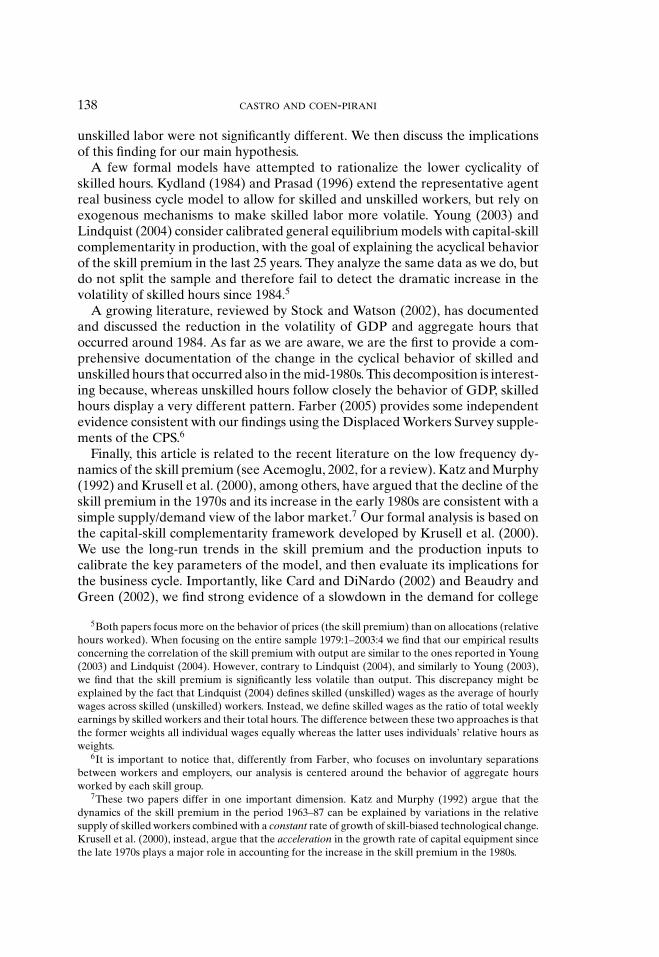
We first partition the sample into 240 demographic groups. Demographicgroups are constructed using information on individuals’ sex, age, race,and education. First, for each quarter and for each demographic groupin our partition, we compute total weekly hours worked by individuals inthat group and their associated total earnings by summing up the individ-ual data. This amounts to assuming that individuals in each demographicgroup are perfect substitutes. We then divide total weekly earnings bytotal hours to obtain a measure of the hourly wage rate for that demo-graphic group. A group’s average hourly wage rate across all quarters isthen used, together with its sampling weight, to aggregate hours of workacross demographic groups. Total hours for skilled (unskilled) workers ina quarter are then defined as the weighted sum of total hours worked bydemographic groups composed by skilled (unskilled) individuals. Thesetwo series are reported in Figure 1. This figure documents an increase intotal hours throughout the sample period, at a significantly higher pacefor skilled workers. As suggested above, the main driving force was anincrease in the relative employment of skilled workers.

(iii) Average Weekly Working Hours. This variable is defined as Total Hoursdivided by Employment.

(iv) Hourly Wage. To define the hourly wage for skilled (unskilled) individualswe divide the sum of weekly earnings across the appropriate demographicgroups by our measure of total hours.

(v) Skill Premium. The skill premium is defined as the ratio of hourly wagesof skilled and unskilled workers. It is also represented in Figure 1. Thefigure documents a steady increase in the skill premium in the last twodecades, 22% between 1979:1 and 2003:4, with a slower growth rate in the1990s.

2.2. Stylized Facts. In what follows we are interested in the behavior of thequantity and price variables described above at the business cycle frequency.The raw series of all the variables considered in this section, like the ones inFigure 1, typically display a trend, seasonal cycles, and fluctuations with higherfrequencies than standard business cycles. In order to deseasonalize the series weuse the Census Bureau’s seasonal adjustment program, X12. In order to smooththe high frequency variations in the data, we applied a centered five quarters mov-ing average to the seasonally adjusted series.11 Finally, each series is detrendedusing the Hodrick–Prescott (HP) filter with parameter 1600, as is standard withquarterly data.

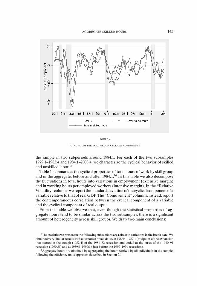
Figure 2 shows the cyclical behavior of total hours per skill group, together withreal GDP. A quick glance at this figure reveals a clear difference between the

11This high frequency noise is likely due to measurement error. In fact, it becomes more significant

for more disaggregated time series, such as the ones underlying Tables 7 and 9, which are based upon

a smaller number of observations. Filtering away the high frequency fluctuations in the data does not

significantly affect the stylized facts emphasized in this section. The tables presented in this section,

obtained using deseasonalized but unfiltered data, are available from the authors upon request.


FIGURE 1

TOTAL HOURS AND SKILL PREMIUM

first and the second halves of our sample. In the first two NBER recessions (1980and 1981–82), the unskilled labor input is strongly procyclical and essentially asvolatile as output.12 The skilled labor input, instead, is not very volatile. The lasttwo recessions (1990–91 and 2001) display a remarkably different pattern: Theskilled input becomes strongly procyclical and essentially as volatile as both GDPand the unskilled input.

This dramatic increase in the absolute volatility of skilled labor is remark-able because, as documented by McConnell and Perez-Quiros (2000), Stock andWatson (2002), and many others, the volatility of most macroeconomic aggregateshas declined since the mid-1980s.

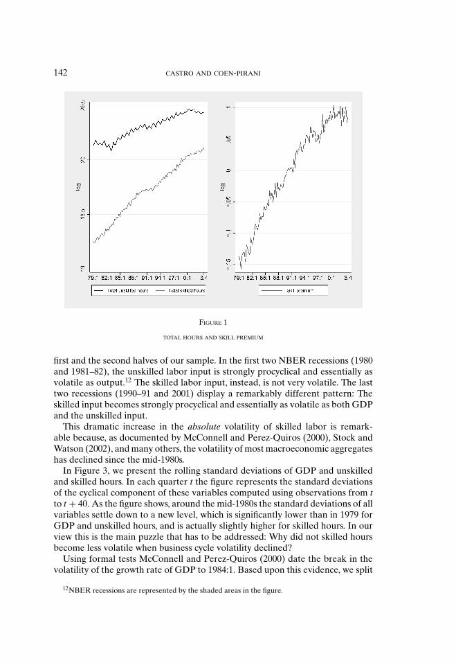
In Figure 3, we present the rolling standard deviations of GDP and unskilledand skilled hours. In each quarter t the figure represents the standard deviationsof the cyclical component of these variables computed using observations from tto t + 40. As the figure shows, around the mid-1980s the standard deviations of allvariables settle down to a new level, which is significantly lower than in 1979 forGDP and unskilled hours, and is actually slightly higher for skilled hours. In ourview this is the main puzzle that has to be addressed: Why did not skilled hoursbecome less volatile when business cycle volatility declined?

Using formal tests McConnell and Perez-Quiros (2000) date the break in thevolatility of the growth rate of GDP to 1984:1. Based upon this evidence, we split

12NBER recessions are represented by the shaded areas in the figure.


FIGURE 2

TOTAL HOURS PER SKILL GROUP: CYCLICAL COMPONENTS

the sample in two subperiods around 1984:1. For each of the two subsamples1979:1–1983:4 and 1984:1–2003:4, we characterize the cyclical behavior of skilledand unskilled labor.13

Table 1 summarizes the cyclical properties of total hours of work by skill groupand in the aggregate, before and after 1984:1.14 In this table we also decomposethe fluctuations in total hours into variations in employment (extensive margin)and in working hours per employed workers (intensive margin). In the “RelativeVolatility” columns we report the standard deviation of the cyclical component of avariable relative to that of real GDP. The “Comovement” columns, instead, reportthe contemporaneous correlation between the cyclical component of a variableand the cyclical component of real output.

From this table we observe that, even though the statistical properties of ag-gregate hours tend to be similar across the two subsamples, there is a significantamount of heterogeneity across skill groups. We draw two main conclusions:

13The statistics we present in the following subsections are robust to variations in the break date. We

obtained very similar results with alternative break dates, at 1986:4–1987:1 (midpoint of the expansion

that started at the trough (1982:4) of the 1981–82 recession and ended at the onset of the 1990–91

recession (1990:3)) and at 1989:4–1990:1 ( just before the 1990–1991 recession).14Aggregate hours are obtained by aggregating the hours worked by all individuals in the sample,

following the efficiency units approach described in Section 2.1.


FIGURE 3

ROLLING STANDARD DEVIATIONS (40 QUARTERS AHEAD) OF GDP AND UNSKILLED AND SKILLED HOURS

TABLE 1

VOLATILITY AND COMOVEMENT OF TOTAL HOURS, EMPLOYMENT, AND AVERAGE WEEKLY HOURS PER SKILL

GROUP (HOUSEHOLD SURVEY)

Relative volatility Comovement

Variable Skilled Unskilled Aggregate Skilled Unskilled Aggregate

1979:1–1983:4 Total hours 0.37 0.97 0.73 0.61a 0.88a 0.91a

Employment 0.32 0.82 0.67 0.25 0.86a 0.87a

Average weekly 0.18 0.17 0.11 0.78a 0.90a 0.71a

hours of work

1984:1–2003:4 Total hours 1.04 0.90 0.81 0.71a 0.69a 0.80a

Employment 0.93 0.81 0.73 0.66a 0.69a 0.76a

Average weekly 0.30 0.26 0.22 0.45a 0.28b 0.47a

hours of work

NOTES: a and b denote correlations significant at the 1% and 5% level, respectively.

(i) Stylized Fact 1. Before 1984 total hours worked by skilled individuals areprocyclical but not very volatile relative to GDP. After 1984 their relativevolatility nearly triples. This result is driven by an increase in the relativevolatility of skilled employment after 1984.15

15Interestingly, using Canadian household survey data (Labour Force Survey) on skilled and un-

skilled employment for the period 1976:1–2002:4 we have found a similar pattern. Specifically, there


TABLE 2

VOLATILITY AND COMOVEMENT OF THE SKILL PREMIUM AND WAGES PER SKILL GROUP AND IN THE

AGGREGATE (HOUSEHOLD SURVEY)



1979:1–1983:4 Hourly wage 0.75 0.57 0.63 0.29 0.41c 0.41c

Skill premium 0.26 −0.11

1984:1–2003:4 Hourly wage 0.96 0.66 0.74 0.35a 0.27b 0.29a

Skill premium 0.60 0.15

NOTES: a, b, c denote correlations significant at the 1%, 5%, and 10% level, respectively.

(ii) Stylized Fact 2. The cyclical properties of total hours worked by unskilledindividuals remain roughly constant relative to GDP after 1984. Specifi-cally, their relative volatility remains virtually unchanged and close to one.16

Despite the changes in the cyclical behavior of quantities, we do not observea significant change in the behavior of prices. Table 2 summarizes the cyclicalbehavior of wages and the skill premium by skill group and in the aggregate,before and after 1984.

This table shows that, even though the relative price of skilled labor becamemore volatile after 1984, its correlation with GDP is basically zero in both samples.Our main conclusion is thus that:

(iii) Stylized Fact 3. The skill premium is acyclical both before and after 1984.

2.3. Ruling Out Explanations Based on Composition Effects. As mentionedin Section 2.1, we follow an efficiency units approach to aggregate individual hoursdata for skilled and unskilled workers. This procedure allows one to control forcyclical variations in the quality of the labor force. However, it is not sufficientto rule out other types of composition effects due to the fact that the structureof the economy is changing over time. In this section we briefly address the mainconcerns regarding the role of aggregation in explaining the stylized facts of theprevious section. Our conclusion is that these empirical observations are not anartifact of aggregation. For the sake of conciseness, in this section we summarizeour main findings on this issue. The interested reader can find additional detailsand tables in Appendix A.2.

has been a dramatic increase in the volatility and comovement of aggregate employment for college

educated workers in Canada after 1984. Details on these data and on the cyclical properties of labor

in Canada are contained in Appendix A.3.16Unskilled total hours display a one quarter lag with respect to GDP in both subperiods. Notice that

the contemporaneous correlation of GDP with unskilled hours, employment, and especially average

weekly hours drops after 1984.


2.3.1. Sectoral composition. Do the statistics reported in Section 2.2 reflectthe different distribution of skilled and unskilled employment across sectors? Itcould be argued, for example, that the 1980 and 1981–82 recessions mainly affectedthe manufacturing sector, where most of unskilled employment tends to be con-centrated, whereas the subsequent recessions affected relatively more the servicesector, where most of skilled employment tends to be concentrated. To addressthis concern, we constructed an artificial time series for the cyclical componentof skilled labor by imposing that the share of aggregate skilled hours worked ineach one-digit industry is equal to the analogous share for unskilled hours (seeAppendix A.2 for details on this new series). The cyclical properties of this artifi-cial series are very similar to the ones of the original series. In particular, its relativevolatility in the second subperiod is 2.4 times larger than in the first subperiod. Thecomparable figure for the original series is 2.8.17 Thus, even after controlling fordifferences in the composition of hours across sectors, there has been a significantincrease in the relative volatility of skilled hours since 1984.

2.3.2. Occupational composition. Similar to the previous point, it may be pos-sible that Stylized Fact 1 is due to the fact that skilled workers are particularly con-centrated in occupations that have become more cyclical since 1984 or that skilledlabor has become more and more employed in traditionally unskilled occupations.To address these concerns we have computed the volatility and comovement withaggregate GDP of total hours by skill group and one-digit occupation. This disag-gregated analysis (see Table 9 in Appendix A.2) shows that after 1984 skilled totalhours tend to be significantly more volatile and procyclical in all the three majoroccupations for skilled workers. Instead, the cyclical properties of unskilled totalhours in these same occupations do not change in an important way after 1984.We also find that the share of skilled employment in each of the four major occu-pations for unskilled workers (lines 3 to 6 in Table 9) has been remarkably stableduring the sample period. These observations, therefore, do not lend support tothe hypothesis that aggregation effects related to the occupational composition ofthe workforce can explain our results.

2.3.3. Males vs. females. Can the increased volatility of aggregate skilled hoursbe explained by an increase in the labor force participation of women in the last25 years? Our concern is that women’s hours might be more cyclical than men’sdue to their higher elasticity of labor supply. To control for potential compositionaleffects, we restricted attention to the subsample of white males workers aged 31–55. The results of this exercise (see Table 10 in Appendix A.2) not only confirmour Stylized Facts 1 and 2, but also contribute to show that the phenomenon weare documenting affects a category of workers (skilled white males with some

17A related question is whether the increased volatility of skilled hours is due to an increase in their

variances at the sectoral level, or in their covariances. Decomposing the increase in the variance of

total skilled hours relative to GDP into these two components reveals that approximately 70% of this

increase is due to higher sectoral variances and the remaining 30% to higher sectoral covariances.


work experience) that has been traditionally thought of as relatively insulatedfrom business cycle fluctuations.18

2.3.4. Skills vs. education. The share of the labor force accounted for by work-ers with a college degree has increased steadily over the sample period, from 18%in 1979 to 29% in 2003. This trend might have been accompanied by a change inthe distribution of workers’ unobserved skills for at least two reasons: a reductionin the quality of college education over time and/or a change in the pattern ofselection into college education. For both reasons, workers who obtained a col-lege degree in more recent years could have less unobserved skills than collegeeducated workers from older cohorts. This composition effect might explain thehigher volatility of aggregate hours worked by college educated individuals after1984. In order to partially address this concern, we changed our definition of skilledlabor. Skilled workers are now those with at least a master’s degree (or with atleast 18 years of school attendance), and unskilled workers are all the remaining.Underlying this approach is the idea that the composition effects mentioned abovewould mostly affect the unobserved quality of individuals who have obtained acollege degree after 1984, and relatively less the quality of individuals obtaininga master degree. We repeated the analysis of Table 1 using this alternative defini-tion of skill (see Table 11 in Appendix A.2). The results clearly indicate that thestandard deviation of aggregate skilled hours has risen dramatically after 1984,even adopting this more restrictive definition of skills.19 As further evidence thatthere has not been a reduction in the “skill content” of a college degree relativeto a high school one, Card and DiNardo (2002) document that the rise in the skillpremium since the early 1980s has been concentrated among younger workersaged 26–35. Thus, it seems unlikely that changes in the distribution of unobservedskills can explain our Stylized Fact 1.

In conclusion, the analysis of this section shows that the increased volatility ofaggregate skilled hours is likely not an artifact of aggregation, but rather a robuststylized fact. In the rest of the paper we propose and empirically evaluate someexplanations for this fact.

3. CAPITAL-SKILL COMPLEMENTARITY AND THE BUSINESS CYCLE

In this section, we perform an analysis of our stylized facts and suggest a candi-date explanation for them. Since the cyclical properties of unskilled hours, relative

18Focusing on female, rather than male, workers yields qualitatively similar results. The relative

standard deviation of total hours increases for both skilled and unskilled females, but proportionally

more so for the former group. The relative standard deviation of total hours for skilled females goes

from 0.61 to 0.99, whereas for unskilled females it goes from 0.76 to 0.92. The correlation between total

hours worked by skilled females and GDP goes from 0.23 before 1984 to 0.52 afterwards, whereas the

analogous correlation for unskilled females declines from 0.72 to 0.59.19Notice that, with this new definition of skilled workers, the relative volatility of skilled labor tends

to be higher than in Table 1. This is likely due to the fact that the measure of aggregate skilled labor

obtained using the “Master” cutoff has to be computed with less observations than the benchmark

measure in Table 1. As pointed out in footnote 55 of Appendix A.2, we think that in this case it is more

meaningful to look at the ratio of post-to-pre 1984 relative volatilities, rather than at their absolute

levels.


to GDP, have not changed significantly during the sample period (Stylized Fact 2),our goal, in what follows is to try to explain Stylized Fact 1:

� In the pre-1984 period, skilled hours are significantly less volatile thanunskilled hours and GDP.

� In the post-1984 period, skilled hours become roughly as volatile as un-skilled hours and GDP.

We begin with a description of our framework, which is further discussed inSection 3.2. Section 3.3 illustrates qualitatively our hypothesis, while Section 4develops its quantitative implications.

3.1. Framework. We follow Krusell et al. (2000) and derive the relative de-mand for skilled and unskilled workers from this production function:

yt = zt kαst

[μuσ

t + (1 − μ)(λkρ

et + (1 − λ)sρt

)σ/ρ](1−α)/σ,(1)

where yt denotes output, zt total factor productivity, and ut and st total unskilledand skilled hours, respectively. kst and ket are, respectively, the stock of capitalstructures and capital equipment. The distinction between the two types of cap-ital will be important for our quantitative analysis: They have been growing atsignificantly different rates, and equipment is likely to exhibit the highest degreeof complementarity with skilled labor.

In this production function, the direct elasticity of substitution between un-skilled labor and either skilled labor or capital equals 1/(1 − σ ), and the directelasticity of substitution between skilled labor and capital equals 1/(1 − ρ).

Assuming perfectly competitive factor markets, profit maximization yields theinverse relative demand for skilled workers:

ωt = (1 − μ) (1 − λ)

μ

(st

ut

)σ−1 [λ

(ket

st

)ρ

+ 1 − λ

] σ−ρ

ρ

,(2)

where ωt denotes the skill premium:

ωt = wst

wut,

and wjt is the real hourly wage of a worker of type j = s, u. It is important to notice

that Equation (2) holds even in the absence of perfect competition in the outputmarket,20 and it is consistent with different sources of business cycle fluctuations,

20In general, the labor demand for each type of worker equals

wjt =

(1 + m−1

t

)MPjt , j = s, u,

where mt denotes the price elasticity of output demand faced by the firm, and MPjt is the (physical)

marginal product of factor j. If the output market is competitive, mt = ∞.


either productivity or monetary shocks. In this sense, our insights apply both toReal Business Cycle and to New Keynesian models.

Equation (2) has been used by Krusell et al. (2000) to study the long-run be-havior of the skill premium. Their exercise consists of using data on the inputratios st/ut and ket/st, together with estimates of the production function’s param-eters, to predict the low frequency variations in the skill premium over the period1963–92.

Our main focus is, instead, on the cyclical dynamics of the skill premium andthe input ratios. In order to introduce a relative supply for skilled labor at thecyclical frequency, we decompose each variable xt in Equation (2) into a trendcomponent, xT

t , and cyclical component xct . The latter is defined as

xct = xt

xTt

.

Using this notation, Equation (2) can be rewritten as

ωct = (1 − μ) (1 − λ)

μωTt

(sc

t sTt

uct uT

t

)σ−1 [λ

(kc

et kTet

sct sT

t

)ρ

+ 1 − λ

] σ−ρ

ρ

.

The relationship between the cyclical component of the skill premium, ωct , and

the ratios of the cyclical components of skilled and unskilled total hours sct /uc

t isrepresented in Figure 4. In drawing this curve we take as given the trends ωT

t ,sT

t /uTt , kT

et/sTt , as well as the ratio of the cyclical components of capital and skilled

labor kcet/sc

t . This relative demand curve is downward sloping in the space (sct /uc

t ,ωc

t ) because a firm is willing to hire more skilled hours only at a lower relativewage (relative quantity effect). Moreover, if σ > ρ, the production function (1)displays capital-skill complementarity and an increase in kc

et/sct gives rise to an

outward shift of this curve (capital-skill complementarity effect).21,22

We add to Figure 4 a perfectly elastic relative supply of skilled hours at thebusiness cycle frequency:

ωct = v.

This yields a skill premium that does not display any cyclical variations, which isconsistent with the empirical evidence discussed in Section 2.1. From a theoreticalpoint of view, a perfectly elastic relative supply at the business cycle frequencywould emerge in an indivisible labor model with skilled and unskilled workers,

21Fallon and Layard (1975) show that capital-skill complementarity is in fact characterized by the

same condition on the parameters of the production function (1) even if alternative definitions of the

elasticity of substitution are used, namely either the elasticity of complementarity or the Hicks–Allen

elasticity of substitution. Differently from the notion of direct elasticity of substitution used in the text,

these alternatives yield elasticities that depend upon input shares, as well as on production function

parameters.22Krusell et al. (2000) estimate Equation (2), given the observed behavior of the labor inputs and

capital stock in the U.S. for the period 1963–92, and find support for the hypothesis that σ > ρ.


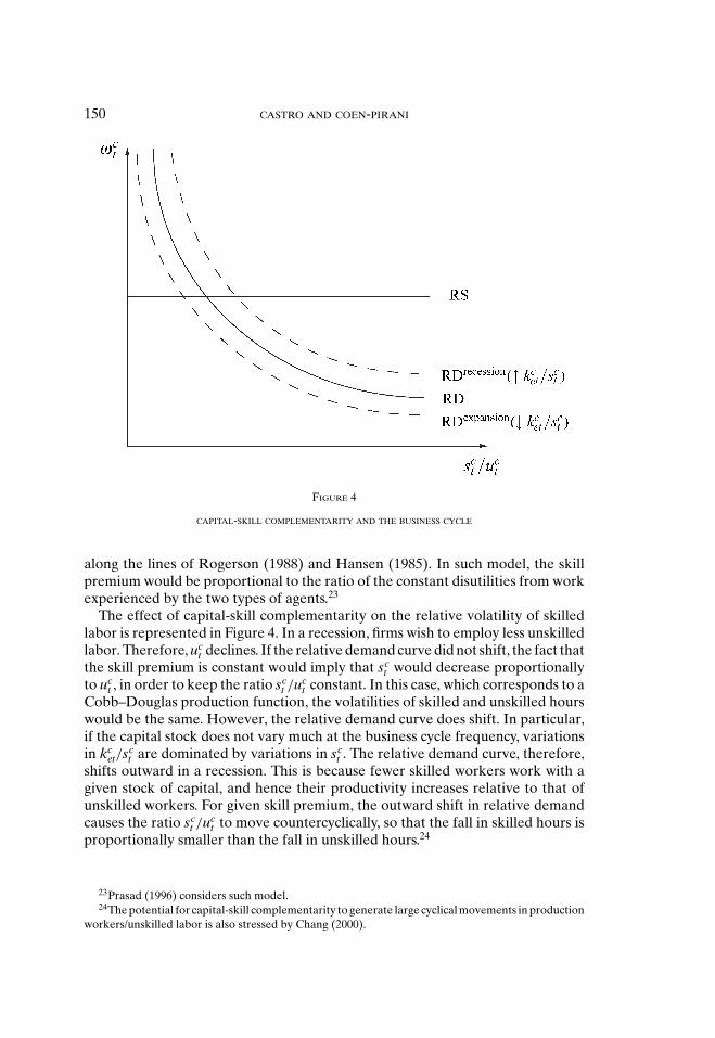
FIGURE 4

CAPITAL-SKILL COMPLEMENTARITY AND THE BUSINESS CYCLE

along the lines of Rogerson (1988) and Hansen (1985). In such model, the skillpremium would be proportional to the ratio of the constant disutilities from workexperienced by the two types of agents.23

The effect of capital-skill complementarity on the relative volatility of skilledlabor is represented in Figure 4. In a recession, firms wish to employ less unskilledlabor. Therefore, uc

t declines. If the relative demand curve did not shift, the fact thatthe skill premium is constant would imply that sc

t would decrease proportionallyto uc

t , in order to keep the ratio sct /uc

t constant. In this case, which corresponds to aCobb–Douglas production function, the volatilities of skilled and unskilled hourswould be the same. However, the relative demand curve does shift. In particular,if the capital stock does not vary much at the business cycle frequency, variationsin kc

et/sct are dominated by variations in sc

t . The relative demand curve, therefore,shifts outward in a recession. This is because fewer skilled workers work with agiven stock of capital, and hence their productivity increases relative to that ofunskilled workers. For given skill premium, the outward shift in relative demandcauses the ratio sc

t /uct to move countercyclically, so that the fall in skilled hours is

proportionally smaller than the fall in unskilled hours.24

23Prasad (1996) considers such model.24The potential for capital-skill complementarity to generate large cyclical movements in production

workers/unskilled labor is also stressed by Chang (2000).


3.2. Discussion. Before proceeding, it is useful to discuss some aspects ofour modelling strategy.

We chose not to use a full-fledged general equilibrium model, but rather focuson the relative supply and demand equations that characterize the equilibrium ofthe labor market in the short run. We use this equilibrium condition to ask thefollowing question: Given the long-run dynamics of the skill premium, and theobserved behavior of unskilled hours and capital equipment, how much of theshort-run behavior of skilled hours is accounted for by the model?

This type of approach has been employed in different areas of macroeconomics.For example, within the context of a representative agent model, Prescott (2004)exploits the equality between the marginal product of labor and the marginalrate of substitution between consumption and leisure to derive an expression forlabor supply as a function of aggregate consumption, output, and the labor taxrate. He then replaces U.S. and European data in this expression and derivespredicted series for per-capita hours worked in these countries. Similarly, in theconsumption-based asset pricing literature (see, e.g., Kocherlakota, 1996) it iscommon to use a parameterized version of the Euler equation, together with theactual series for aggregate consumption, in order to derive predicted series forasset returns.

A second motivation for focusing exclusively on the labor market equilibriumis that it is not obvious how to make a general equilibrium business cycle modelconsistent with the “nonbalanced growth” kind of dynamics exhibited by the seriesfor capital, the two labor inputs, and the skill premium. For example, along thebalanced growth path of a general equilibrium version of our model, the skillpremium and the relative quantities of inputs would have to be constant, ratherthan increasing, as in the data.25 We chose not to pursue this approach because,empirically, these trends play an important role, as they allow us to calibrate theparameters of the model (see Section 4).

Instead, this partial equilibrium approach allows us to cleanly connect our ex-ercise with the literature on the long-run behavior of the skill premium.26 In thisliterature, researchers commonly derive a relative demand function for skilledworkers analogous to the one in Equation (2). Then, they take as given the seriesfor the supplies of labor and either derive implications for the dynamics of skill-biased technical change for given behavior of the skill premium (see, e.g., Katzand Murphy, 1992), or obtain predictions for the behavior of the skill premiumfor given behavior of the capital stock (see, e.g., Krusell et al., 2000). In additionto specifying the relative demand for skilled labor, which holds at all frequencies,

25Lindquist (2004) considers a general equilibrium real business cycle model with capital skill

complementarity in production. His model is calibrated with reference to the average ratio of unskilled

to skilled labor and the average skill premium in the sample period 1979–2002. However, these ratios

display significant trends over that period.26In taking this frictionless view of the labor market, we do not intend to minimize the potential

roles played by firm-specific human capital, insurance contracts, search and matching, wage rigidities,

etc. in accounting for the stylized facts of Section 2. Instead, we view our exercise as a first step, based

on the simplest representation of labor market interactions, towards their explanation. In Section 6,

we speculate on some of these possible complementary explanations.


we also specify a perfectly elastic short-run relative supply. It is simple to showthat this would be the case in a stationary business cycle model characterized byindivisible labor (Hansen, 1985). However, as suggested above, we prefer not towork with a stationary version of the model in order to retain the low-frequencyvariations of the series for the skill premium and the production inputs. Underly-ing this approach is the view that the decision of workers of a given educationalbackground to supply more or less hours in response to cyclical variations in realwages is fundamentally different from the decision of whether to acquire moreskills in face of secular changes in the skill premium. We think it is appropriate tostudy the former problem separately from the latter.

3.3. Hypothesis. In order to try to explain our pre- and post-1984 stylizedfacts, it is convenient to derive an analytical expression for the volatility of skilledhours. To do so, first equalize relative supply to relative demand at the businesscycle frequency to obtain

ωTt = (1 − μ) (1 − λ)

μv

(sc

t sTt

uct uT

t

)σ−1 [λ

(kc

et kTet

sct sT

t

)ρ

+ 1 − λ

] σ−ρ

ρ

.(3)

Then, assume for simplicity that there are no low frequency variations in thevariables that enter this equation: ωT

t = ω, sTt = s, uT

t = u, kTet = ke. Last, linearize

Equation (3) to obtain sct as function of uc

t and kcet:

sct = 1

1 + Quc

t + Q1 + Q

kcet ,(4)

where the constant Q is defined as

Q ≡ σ − ρ

1 − σ

λ( ke

s

)ρ

λ( ke

s

)ρ + 1 − λ.(5)

Under the assumption that the covariance between uct and kc

et is zero, it followsfrom Equation (4) that27

var(sct )

var(uct )

=(

1

1 + Q

)2

+(

Q1 + Q

)2 var(kcet )

var(uct )

.(6)

This equation contains our main insights concerning the volatility of skilled laborrelative to unskilled labor. In what follows, we first describe our hypothesis in a

27In the data the correlation between uct and kc

et is equal to 0.36. Here, we set it equal to zero to

simplify our explanation. Of course, in the empirical section of the paper, we allow uct and kc

et to be

positively correlated. See Section 4 for a description of the data for the stock of capital equipment.


qualitative way. In Section 4, we calibrate the model and evaluate each mechanismquantitatively.

3.3.1. Pre-1984 period. In the data the variance of sct is lower than the variance of

uct . From Equation (6), we know that our simple model can qualitatively account

for this fact under two conditions: (1) capital-skill complementarity in production(σ > ρ), implying Q > 0; (2) the capital stock is less volatile than unskilled labor:var(kc

et) < var(uct ). Regarding the latter point, notice that although the stock of

physical capital does not display large variations at the business cycle frequency,the flow of services per unit of time provided by this stock might be significantlyprocyclical, as firms can adjust the work week of capital along the business cy-cle. The reason why we did not allow for cyclical capital utilization in our modelhas to do with the nature of complementarity between skilled workers and cap-ital equipment that we intend to formalize. If skilled workers are needed in or-der to set up and supervise the work of equipment capital, then variations inthe work week of capital will only have limited influence on the demand forskilled workers, while possibly exerting some influence on their average weeklyhours.

Notice that, ceteris paribus, if var(kcet)/var(uc

t ) is low enough, the relative volatil-ity of skilled labor declines with an increase in Q.28 In turn Q increases with thedegree of capital skill complementarity, measured by σ − ρ. With a Cobb–Douglasproduction function, the term Q would be equal to zero and our model would pre-dict that var(sc

t ) = var(uct ). The mechanism emphasized here has been first pointed

out by Oi (1962) and Rosen (1968) to explain the lower cyclicality of skilled labor,but, to our knowledge, it has not been quantitatively evaluated.

3.3.2. Post-1984 period. In the post-1984 period, the variance of sct increases

significantly relative to the variance of uct . The variances of these two variables

are approximately equal after 1984. In what follows we focus on three effects thatcan potentially explain this change.

(1) Reduction in degree of capital-skill complementarity. Our main candidateexplanation for the increase in the relative volatility of skilled hours isrepresented by a reduction in the degree of capital skill complementarity.Mechanically, a reduction in σ − ρ leads to a reduction in Q, which tendsto increase var(sc

t )/var(uct ). The key question is, of course, whether and

when such decline in the degree of capital-skill complementarity tookplace. As we discuss in more detail in the next section, this hypothesisis consistent with the long-run behavior of the skill premium ωT

t and therelative inputs sT

t /uTt and kT

et/sTt since the late 1980s. During this period,

and relative to the early 1980s, the growth rate of the skill premium slowsdown considerably. This deceleration is accompanied by a higher growthrate of the stock of capital equipment relative to skilled hours, and by aslowdown in the growth rate of sT

t /uTt . In order to reconcile these facts

28Since capital is not very cyclical, the relevant condition is verified in the data.


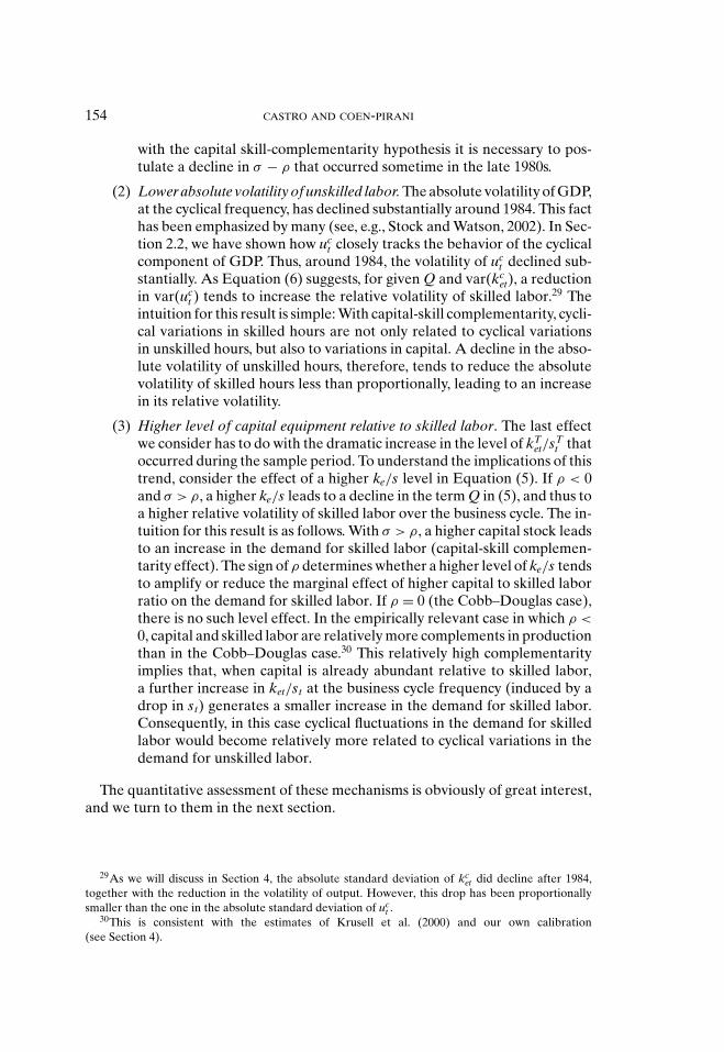
with the capital skill-complementarity hypothesis it is necessary to pos-tulate a decline in σ − ρ that occurred sometime in the late 1980s.

(2) Lower absolute volatility of unskilled labor. The absolute volatility of GDP,at the cyclical frequency, has declined substantially around 1984. This facthas been emphasized by many (see, e.g., Stock and Watson, 2002). In Sec-tion 2.2, we have shown how uc

t closely tracks the behavior of the cyclicalcomponent of GDP. Thus, around 1984, the volatility of uc

t declined sub-stantially. As Equation (6) suggests, for given Q and var(kc

et), a reductionin var(uc

t ) tends to increase the relative volatility of skilled labor.29 Theintuition for this result is simple: With capital-skill complementarity, cycli-cal variations in skilled hours are not only related to cyclical variationsin unskilled hours, but also to variations in capital. A decline in the abso-lute volatility of unskilled hours, therefore, tends to reduce the absolutevolatility of skilled hours less than proportionally, leading to an increasein its relative volatility.

(3) Higher level of capital equipment relative to skilled labor. The last effectwe consider has to do with the dramatic increase in the level of kT

et/sTt that

occurred during the sample period. To understand the implications of thistrend, consider the effect of a higher ke/s level in Equation (5). If ρ < 0and σ > ρ, a higher ke/s leads to a decline in the term Q in (5), and thus toa higher relative volatility of skilled labor over the business cycle. The in-tuition for this result is as follows. With σ > ρ, a higher capital stock leadsto an increase in the demand for skilled labor (capital-skill complemen-tarity effect). The sign of ρ determines whether a higher level of ke/s tendsto amplify or reduce the marginal effect of higher capital to skilled laborratio on the demand for skilled labor. If ρ = 0 (the Cobb–Douglas case),there is no such level effect. In the empirically relevant case in which ρ <

0, capital and skilled labor are relatively more complements in productionthan in the Cobb–Douglas case.30 This relatively high complementarityimplies that, when capital is already abundant relative to skilled labor,a further increase in ket/st at the business cycle frequency (induced by adrop in st) generates a smaller increase in the demand for skilled labor.Consequently, in this case cyclical fluctuations in the demand for skilledlabor would become relatively more related to cyclical variations in thedemand for unskilled labor.

The quantitative assessment of these mechanisms is obviously of great interest,and we turn to them in the next section.

29As we will discuss in Section 4, the absolute standard deviation of kcet did decline after 1984,

together with the reduction in the volatility of output. However, this drop has been proportionally

smaller than the one in the absolute standard deviation of uct .

30This is consistent with the estimates of Krusell et al. (2000) and our own calibration

(see Section 4).


4. QUANTITATIVE ANALYSIS

In this section we calibrate the model and undertake a quantitative analysis ofthe three mechanisms illustrated in Section 3. In Section 4.1, we consider two ofthese mechanisms: the lower volatility of unskilled hours and the higher capital-skilled labor ratio that characterize the post-1984 period. To do so, the parametersof the equilibrium relationship (3) are calibrated using data for the whole 1979:1–2002:4 period.31 For this reason, we label this exercise “Constant Parameters.”

In Section 4.2, we evaluate the effect of our main mechanism, a reduction inthe degree of capital-skill complementarity. This “Changing Parameters” exerciseis motivated by the difficulty faced by the version of the model with constantparameters in reconciling the lower growth rate of the skill premium in the 1990swith the simultaneous acceleration in the growth rate of the capital-skilled hoursratio.

4.1. The Lower Volatility of Unskilled Hours and the Higher Capital-Skilled La-bor Ratio. The center of our quantitative analysis is the labor market equilibriumcondition (3), which we reproduce below for convenience:

ωTt = (1 − μ) (1 − λ)

μv

(st

ut

)σ−1 [λ

(ket

st

)ρ

+ 1 − λ

] σ−ρ

ρ

.(7)

In Figure 5, we plot the variable ωt and in Figure 6 the variables st/ut andket/st.

32 The series for capital equipment is from Cummins and Violante (2002).33

We interpolate their yearly data to obtain quarterly observations, by imposing aconstant quarterly rate of growth within each year.

Figures 5 and 6 are to be interpreted jointly in terms of Equation (7). Over theentire sample period 1979:1–2002:4, the skill premium and the ratio of skilled tounskilled hours display an upward trend. Given the increase in the ratio of thestock of capital equipment to skilled hours, these two trends can only be recon-ciled, within our framework, by the existence of capital-skill complementarity inproduction.

31Notice that in order to calibrate the model, we use only data up to 2002:4. The reason is that,

although the MORG data set extends until 2003:4, the series for capital equipment is not available for

2003.32The key feature of these series that we wish to emphasize for the purposes of the exercise in this

section is that they all display upward trends. In the next section we will explore the fact that these

trends have in fact changed over time.33The capital equipment series is based upon the Cummins and Violante (2002) series of quality-

adjusted equipment prices. The latter extrapolates Gordon’s (1990) quality-adjusted series, which span

only the 1947–1983 period, until 2000. We extrapolate the Cummins–Violante series to the year 2002.

In order to compute the growth rate of the stock of equipment from 2000 to 2003, we compute the

growth rate of the series published by the BEA and add to it the average amount by which the growth

rate of the Cummins–Violante series exceeds the published data over the period 1979–2000.


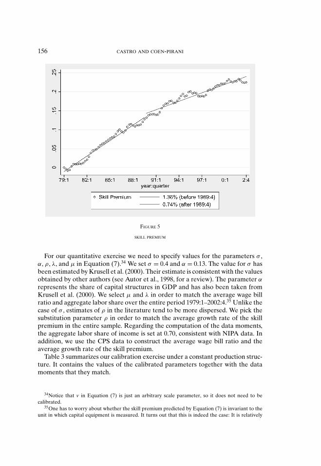
FIGURE 5

SKILL PREMIUM

For our quantitative exercise we need to specify values for the parameters σ ,α, ρ, λ, and μ in Equation (7).34 We set σ = 0.4 and α = 0.13. The value for σ hasbeen estimated by Krusell et al. (2000). Their estimate is consistent with the valuesobtained by other authors (see Autor et al., 1998, for a review). The parameter α

represents the share of capital structures in GDP and has also been taken fromKrusell et al. (2000). We select μ and λ in order to match the average wage billratio and aggregate labor share over the entire period 1979:1–2002:4.35 Unlike thecase of σ , estimates of ρ in the literature tend to be more dispersed. We pick thesubstitution parameter ρ in order to match the average growth rate of the skillpremium in the entire sample. Regarding the computation of the data moments,the aggregate labor share of income is set at 0.70, consistent with NIPA data. Inaddition, we use the CPS data to construct the average wage bill ratio and theaverage growth rate of the skill premium.

Table 3 summarizes our calibration exercise under a constant production struc-ture. It contains the values of the calibrated parameters together with the datamoments that they match.

34Notice that v in Equation (7) is just an arbitrary scale parameter, so it does not need to be

calibrated.35One has to worry about whether the skill premium predicted by Equation (7) is invariant to the

unit in which capital equipment is measured. It turns out that this is indeed the case: It is relatively


FIGURE 6

EQUIPMENT-SKILL AND SKILLED-UNSKILLED INPUT RATIOS

TABLE 3

CALIBRATION UNDER CONSTANT PARAMETERS

Period Parameters Values Target moments Values

1979:1–2003:4 λ 0.73 Average labor share in GDP 0.70

μ 0.54 Average wage bill ratio 0.56

ρ −0.88 Average yearly growth rate of skill premium 1.06%

To evaluate the performance of the model, we use the actual series for ut, ket, andωT

t (computed as the HP-filter trend of ωt ) together with the calibrated parameters(Table 3) in Equation (7), to obtain a predicted series st for skilled hours. We thenHP-filter st to extract its cyclical component sc

t . Figure 7 plots the actual series forst together with st . Figure 8 reports sc

t , together with the the cyclical componentsof output and actual total skilled hours.

Table 4 contains the cyclical properties of skilled hours predicted by our model,before and after 1984. This is our “benchmark” exercise under constant parame-ters, when both effects considered in this section are at work.

easy to show that different measurement units are fully absorbed by the share parameters λ and μ in

our calibration.


FIGURE 7

MODEL FIT FOR THE TOTAL SKILLED HOURS UNDER CONSTANT PARAMETERS

In interpreting these results recall that, with no capital-skill complementarityin production (σ = ρ), the ratio of the standard deviations of skilled and unskilledhours would equal one in both subperiods.36 The existence of capital-skill com-plementarity in production, by itself, explains why the relative standard deviationof skilled hours is significantly smaller than one before 1984.

After 1984, the relative standard deviation of skilled hours increases by 17percentage points (from 0.61 to 0.79), which is about a quarter of the increaseobserved in the data. This change is due to the two effects considered in thissection. First, the absolute volatility of the cyclical component of unskilled hours(uc

t ) has declined dramatically after 1984, whereas the volatility of the cyclicalcomponent of capital equipment (kc

et) did not change in a significant way overthe sample period. In the data, std(kc

et)/std(uct ) increased from 0.50 before 1984:1

to 0.91 after this date. This fact in conjunction with capital-skill complementarityimplies that, as explained in Section 3, the volatility of skilled hours will dropproportionally less than the volatility of unskilled hours and GDP. Second, theratio ket/st has increased over the sample period, especially in the 1990s, when itsgrowth rate more than doubled. If ρ < 0, as in our benchmark calibration, thisincrease should have increased the relative volatility of skilled hours.

36As a consequence, the volatility of skilled hours relative to GDP would also be approximately

equal to one in both subperiods.


FIGURE 8

MODEL PERFORMANCE UNDER CONSTANT PARAMETERS: CYCLICAL COMPONENTS

TABLE 4

QUANTITATIVE RESULTS UNDER CONSTANT PARAMETERS


Total hours Skilled Unskilled Skilled Unskilled

1979:1–1983:4 Data 0.37 0.97 0.61 0.88

Benchmark 0.61 0.63

1984:1–2002:4 Data 1.05 0.91 0.73 0.74

Benchmark 0.79 0.69

Constant ket/st after 1984 0.76 0.69

In order to get a sense of the relative contribution of each of these two effects,we have performed a simple experiment with Equation (4). For given coefficientQ, and for given actual series for the cyclical components of unskilled hours andcapital equipment, this equation can be used to obtain a predicted series for thecyclical component of skilled hours. We have computed the value of the coeffi-cient Q such that the predicted series for skilled hours displays a relative standarddeviation for the period 1979:1–1983:4 equal to the one predicted by the bench-mark case (i.e., 0.61). The relative standard deviation of skilled hours after 1983:4obtained using this procedure is reported in Table 4 under the label “Constantket/st after 1984”. This figure, 0.76, represents the relative volatility of skilled hours


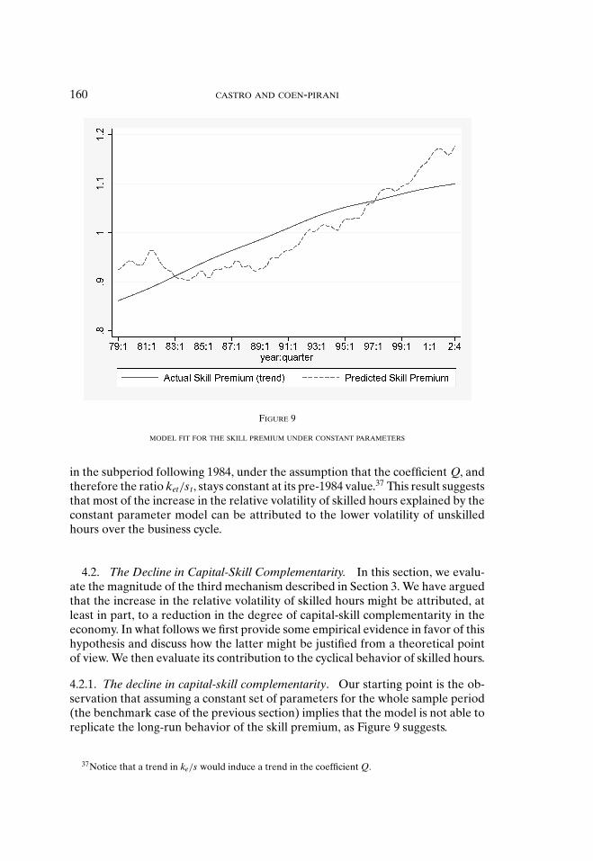
FIGURE 9

MODEL FIT FOR THE SKILL PREMIUM UNDER CONSTANT PARAMETERS

in the subperiod following 1984, under the assumption that the coefficient Q, andtherefore the ratio ket/st, stays constant at its pre-1984 value.37 This result suggeststhat most of the increase in the relative volatility of skilled hours explained by theconstant parameter model can be attributed to the lower volatility of unskilledhours over the business cycle.

4.2. The Decline in Capital-Skill Complementarity. In this section, we evalu-ate the magnitude of the third mechanism described in Section 3. We have arguedthat the increase in the relative volatility of skilled hours might be attributed, atleast in part, to a reduction in the degree of capital-skill complementarity in theeconomy. In what follows we first provide some empirical evidence in favor of thishypothesis and discuss how the latter might be justified from a theoretical pointof view. We then evaluate its contribution to the cyclical behavior of skilled hours.

4.2.1. The decline in capital-skill complementarity. Our starting point is the ob-servation that assuming a constant set of parameters for the whole sample period(the benchmark case of the previous section) implies that the model is not able toreplicate the long-run behavior of the skill premium, as Figure 9 suggests.

37Notice that a trend in ke/s would induce a trend in the coefficient Q.


The principal reason for this failure is that the trends in the skill premium andthe input ratios appear to change sometime around the late 1980s. Figure 5 shows adecline in the average growth rate of the skill premium between the 1979:1–1989:3and 1989:4–2002:4 subperiods (the reason for splitting the sample around 1989:4for the purpose of looking at the long-run trends will become clear later in thissection).

In the first subperiod, the skill premium has grown, on average, at a rate of1.36% per year, and in the second period it has grown at an average rate of 0.74%per year. Figure 6 depicts the evolution of the relative inputs ket/st and st/ut. Thisfigure shows a substantial acceleration after 1989:3 in the growth rate of ket/st

(from 2.69% to 6.19% per year) and a contemporaneous slowdown in the growthof st/ut (from 2.89% to 1.89% per year).38 These observations accord well withthe empirical evidence presented by Card and DiNardo (2002) and Beaudry andGreen (2002), who also notice that the skill premium has grown at a significantlysmaller rate after about 1987 with respect to the previous seven years, despite anacceleration in the growth rate of the stock of capital equipment.

The evolution of ket/st and st/ut since the late 1980s represents a challengeto the view that the long-run behavior of the skill premium in the 1980s and1990s can be explained using a production structure characterized by capital-skillcomplementarity and constant parameters. The latter would have predicted afaster, rather than a slower, increase in the skill premium since 1989, because thefaster growth in ket/st and the slower growth in st/ut should have made skilledlabor relatively more productive than in the first subperiod (see also Figure 9).Instead, Figure 5 clearly tells otherwise.39

Our view is that this evidence may point to a reduction in the degree of com-plementarity in production between skilled labor and capital equipment startingfrom the late 1980s. The lower degree of capital-skill complementarity would thencontribute to explain the increase in the relative volatility of skilled hours overthe business cycle.

To evaluate the importance of this effect for the cyclical behavior of skilledhours, we follow a simple approach, and assume a once-and-for-all decline inσ − ρ in the production function (1). We view this modelling approach more asa convenient short-cut than a rigorous model of the underlying phenomena, aswe share economists’ reluctance to base their theories on changes in “structural

38The increase in the growth rate of ket/st can be traced back to a substantial decline in the relative

price of equipment in terms of consumption, brought about by a significant acceleration in the tech-

nological progress specific to the production of capital equipment goods. In part as a consequence of

this fact, investment in equipment has accelerated in the post-1989 period, and most notably in the

late 1990s. This is consistent with anecdotal evidence suggesting that the 1990s were a boom period in

terms of investment in equipment.39Figures 9 and 7 are obviously closely related, as they are two different ways of conveying the same

information. In the constant production structure model, the sharp increase in capital equipment that

took place during the 1990s induces a significant increase in relative productivity of skilled labor, all

else constant. Since the actual s/u ratio does not grow any faster in the 1990s, this must lead to a faster

growth in the predicted skill premium (Figure 9). Similarly, since the actual skill premium does not

grow any faster in the 1990s, this must lead to a faster growth in predicted skilled employment (Figure

7).


parameters” such as σ and ρ. A full-fledged model should be able to capturethe decline in capital-skill complementarity as a slowly evolving process spanningseveral years, presumably due to the diffusion and routinization of computersand information technologies, and reaching maturity around the late 1980s. Inthis regard, Katz (1999, p. 17) has interpreted the slowdown in the growth ofthe relative demand for skill since the late 1980s, as reflecting a “maturing ofthe computer revolution,” whereby “as technologies diffuse and become moreroutinized the comparative advantage of the highly skilled declines.” Along thesame line, Blanchard (2003, p. 181) conjectures that “it is likely that computers willbecome easier and easier to use in the future, even by low skill workers. Computersmight even replace high-skill workers, those workers whose skills involve primarilythe ability to compute or to memorize.” The theoretical model that, perhaps, bestcaptures this view is the one developed by Greenwood and Yorokoglu (1997) todescribe the effects of the faster decline in the price of equipment since 1974 onthe relative demand for skilled labor. In this model, a technological revolution isfollowed by a transitory increase in the demand for skilled labor that is needed toimplement the new technologies. Afterwards, as the latter have been adopted andimplemented, the relative demand for skilled labor declines towards its originalsteady state level. Although we agree that it would be more satisfactory to usea version of Greenwood and Yorokoglu’s (1997) model as a foundation for ourempirical exercise, we do not pursue this route because of the difficult task ofaugmenting the latter with business cycle fluctuations.

4.2.2. Business cycle implications. In order to evaluate the importance of theevidence described above for the cyclical properties of skilled labor, we recalibratethe model allowing for a different degree of capital-skill complementarity after acertain break date in the late 1980s.

In order to set values for the model’s parameters and determine a precise breakdate, we proceed as follows. First, for a given break date T, we assume that whereasthe parameters ρ, μ, and λ of the production function (1) may take on differentvalues before and after T, the parameters α and σ remain instead unchanged overthe entire sample period. The values of ρ, μ, and λ for the subperiod precedingT are set exactly as in Section 4.1, in order to match the average labor share, theaverage wage bill ratio, and the average growth rate of the skill premium between1979:1 and T. The values of ρ, μ, and λ for the subperiod following T are setin an analogous way. For given set of parameters, we then select the break dateT that minimizes the sum of squared errors between the trend in the actual skillpremium, ωT , and the skill premium predicted by the model. This procedure yieldsT = 1989:3 as the break date.

The results of this calibration exercise are summarized in Table 5. Notice, inparticular, how the calibrated elasticity of substitution between skilled labor andcapital equipment is now much lower before 1984, and much higher after 1984,compared to the benchmark case of Table 3.

Before proceeding, a few observations are in order. First, the assumption thatthe decline in σ − ρ is due to an increase in ρ, rather than a decrease in σ , ismotivated by the idea that, as computers and information technologies become


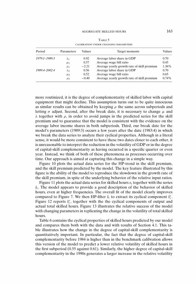
TABLE 5

CALIBRATION UNDER CHANGING PARAMETERS

Period Parameters Values Target moments Values

1979:1–1989:3 λ1 0.92 Average labor share in GDP 0.70

μ1 0.57 Average wage bill ratio 0.45

ρ1 −2.21 Average yearly growth rate of skill premium 1.36%

1989:4–2002:4 λ2 0.56 Average labor share in GDP 0.70

μ2 0.52 Average wage bill ratio 0.65

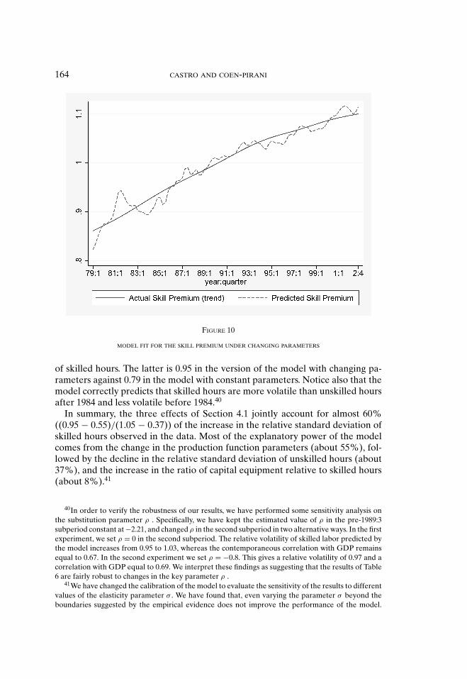
ρ2 −0.40 Average yearly growth rate of skill premium 0.74%

more routinized, it is the degree of complementarity of skilled labor with capitalequipment that might decline. This assumption turns out to be quite innocuousas similar results can be obtained by keeping ρ the same across subperiods andletting σ adjust. Second, after the break date, it is necessary to change μ andλ together with ρ, in order to avoid jumps in the predicted series for the skillpremium and to guarantee that the model is consistent with the evidence on theaverage labor income shares in both subperiods. Third, our break date for themodel’s parameters (1989:3) occurs a few years after the date (1983:4) in whichwe break the data series to analyze their cyclical properties. Although in a literalsense, it would be more consistent to have these two dates closer to each other, itis unreasonable to interpret the reduction in the volatility of GDP or in the degreeof capital-skill complementarity as having occurred in a specific quarter or evenyear. Instead, we think of both of these phenomena as processes occurring overtime. Our approach is aimed at capturing this change in a simple way.

Figure 10 plots the actual data series for the HP-trend in the skill premium,and the skill premium predicted by the model. The key feature illustrated by thisfigure is the ability of the model to reproduce the slowdown in the growth rate ofthe skill premium, in spite of the underlying behavior of the relative input ratios.

Figure 11 plots the actual data series for skilled hours st together with the seriesst . The model appears to provide a good description of the behavior of skilledhours, even at higher frequencies. The overall fit of the model clearly improvescompared to Figure 7. We then HP-filter st to extract its cyclical component sc

t .Figure 12 reports sc

t , together with the the cyclical components of output andactual total skilled hours. Figure 13 illustrates the relative success of the modelwith changing parameters in replicating the change in the volatility of total skilledhours.

Table 6 contains the cyclical properties of skilled hours predicted by our modeland compares them both with the data and with results of Section 4.1. This ta-ble illustrates how the change in the degree of capital-skill complementarity isquantitatively important. In particular, the fact that the degree of capital-skillcomplementarity before 1984 is higher than in the benchmark calibration allowsthis version of the model to predict a lower relative volatility of skilled hours inthe first subperiod (0.55 against 0.61). Similarly, the higher degree of capital-skillcomplementarity in the 1990s generates a larger increase in the relative volatility


FIGURE 10

MODEL FIT FOR THE SKILL PREMIUM UNDER CHANGING PARAMETERS

of skilled hours. The latter is 0.95 in the version of the model with changing pa-rameters against 0.79 in the model with constant parameters. Notice also that themodel correctly predicts that skilled hours are more volatile than unskilled hoursafter 1984 and less volatile before 1984.40

In summary, the three effects of Section 4.1 jointly account for almost 60%((0.95 − 0.55)/(1.05 − 0.37)) of the increase in the relative standard deviation ofskilled hours observed in the data. Most of the explanatory power of the modelcomes from the change in the production function parameters (about 55%), fol-lowed by the decline in the relative standard deviation of unskilled hours (about37%), and the increase in the ratio of capital equipment relative to skilled hours(about 8%).41

40In order to verify the robustness of our results, we have performed some sensitivity analysis on

the substitution parameter ρ . Specifically, we have kept the estimated value of ρ in the pre-1989:3

subperiod constant at −2.21, and changed ρ in the second subperiod in two alternative ways. In the first

experiment, we set ρ = 0 in the second subperiod. The relative volatility of skilled labor predicted by

the model increases from 0.95 to 1.03, whereas the contemporaneous correlation with GDP remains

equal to 0.67. In the second experiment we set ρ = −0.8. This gives a relative volatility of 0.97 and a

correlation with GDP equal to 0.69. We interpret these findings as suggesting that the results of Table

6 are fairly robust to changes in the key parameter ρ .41We have changed the calibration of the model to evaluate the sensitivity of the results to different

values of the elasticity parameter σ . We have found that, even varying the parameter σ beyond the

boundaries suggested by the empirical evidence does not improve the performance of the model.


FIGURE 11

MODEL FIT FOR TOTAL SKILLED HOURS UNDER CHANGING PARAMETERS

5. BEFORE 1979: EVIDENCE FROM THE MARCH CPS

The quantitative results of Section 4.2 provide some support for the hypothe-sis that the higher volatility of skilled labor observed in the 1990s might be duein part to a decline in the degree of complementarity between skills and capitalequipment. As observed above, such a decline is consistent with the view, orig-inally advanced by Nelson and Phelps (1966) and more recently by Greenwoodand Yorokoglu (1997), that skilled workers have a comparative advantage in im-plementing and adopting new technologies. According to this interpretation, the“technological revolution” that started in the mid 1970s has been characterizedby a transition period of 10–15 years. During this transition period the demandfor skilled labor accelerated, leading to a fast-growing skill premium and to theacyclicality of skilled labor documented in Section 2.2. After this transition period,starting from the late 1980s, new technologies become more routinized, leadingto a slowdown in the demand for skilled labor. This slowdown is reflected in the

Notice that, given our parsimonious parameterization, σ and the share of structures, α, are the only

parameters that can, in principle, be set exogenously. Reasonable variations in the latter also do not give

rise to noticeably different results from those of Table 6. Although variations in the other, calibrated,

parameters of the model, λ, μ, and ρ, could possibly generate a better fit of the model at the cyclical

frequency, they would also oblige us not to be able to capture some of the low frequency variations in

the data. Given the role played by the latter in disciplining our empirical exercise we did not pursue

this avenue.


FIGURE 12

MODEL PERFORMANCE UNDER CHANGING PARAMETERS: CYCLICAL COMPONENTS

decline in the growth rate of the skill premium and the higher cyclicality of skilledlabor.

If this line of argument is correct, one should expect skilled labor to be relativelyacyclical only during periods of “technological revolutions,” such as the late 1970sand early 1980s. In order to evaluate this prediction of our model, we need toprovide some evidence regarding the cyclical behavior of skilled labor before 1979.Given that the CPS ORG data are available only since that date, we constructmeasures of the aggregate skilled and unskilled labor inputs using annual datafrom the March CPS for the period 1963–2002.

The analysis of Section 2.2 reveals that most of the increase in the volatilityof skilled labor since 1984 is due to a higher volatility of aggregate employment,as opposed to average hours. Thus, for simplicity, we focus exclusively on theextensive margin.42 Aggregate skilled labor in a given year is measured, using theMarch CPS survey, as the aggregate number of weeks worked by individuals witha college degree in that year. Aggregate unskilled labor is defined analogously.43

42Before 1976, the March CPS survey only asks individuals how many weeks they have worked

last year and how many hours they have worked last week. This presents a limitation in computing

a measure of total hours based upon this sample before 1976. Also for this reason we decided to

concentrate on aggregate employment.43To make these data as comparable to the ORG ones in Section 2.2 as possible, we use the same

sample selection criteria described in the Appendix.


FIGURE 13

MODEL PERFORMANCE UNDER CHANGING PARAMETERS: ROLLING STANDARD DEVIATIONS

(40 QUARTERS AHEAD)

Figure 14 represents the HP-filtered series for aggregate skilled and unskilledlabor from the March CPS, together with aggregate GDP.44 Two features of thesedata stand out. First, from 1979 onwards, the cyclical properties of aggregate skilledlabor measured using the March CPS data are very similar to the ones obtainedusing the ORG data, and represented in Figure 2. In particular, aggregate skilledlabor is relatively acyclical in the 1980 and 1981–82 recessions, whereas it is sig-nificantly more volatile afterwards. Second, and more important, the March CPSdata reveal that in the period between 1963 and 1975, skilled labor tends to beroughly as cyclical as unskilled labor.45 In other words, the acyclicality of skilled la-bor is a transitional phenomenon stretching from the mid-1970s to the mid-1980s.This point can be easily seen by considering, in Figure 15, the rolling standard

44We used a smoothing parameter of 6.25, as suggested by Ravn and Uhlig (2002) for annual data.45This fact requires further comment, as few of the authors cited in the Introduction (particularly

Kydland, 1984; Keane and Prasad, 1993) had found skilled labor to be relatively acyclical in earlier

studies. We attribute this apparent discrepancy to the fact that these authors use microdata samples for

the period 1970–80 (Kydland) and 1966–81 (Keane and Prasad) that include information from both the

“high volatility” subperiod 1963–75 and from the “low volatility” subperiod 1976–83. Additionally, in

order to compute measures of the cyclicality of skilled labor, these authors adopt a regression approach

in which the unemployment rate in one year is correlated with workers’ employment status in the same

year. This method fails to account for any leads and lags in the response of skilled labor to cyclical

fluctuations in GDP in the 1963–75 subperiod (see Figure 14).


TABLE 6

QUANTITATIVE RESULTS: EFFECT OF CHANGING CAPITAL-SKILL COMPLEMENTARITY


Total hours Skilled Unskilled Skilled Unskilled

1979:1–1983:4 Data 0.37 0.97 0.61 0.88

Constant parameters 0.61 0.63

Changing parameters 0.55 0.46

1984:1–2002:4 Data 1.05 0.91 0.73 0.74

Constant parameters 0.79 0.69

Changing parameters 0.95 0.67

deviation for skilled and unskilled labor and GDP in the 1963–2002 period. Thefigure clearly suggests that in the earlier as well as in the later parts of this longsample, the volatility of skilled labor was about the same as the volatility of un-skilled labor and GDP. The rolling standard deviation of skilled labor reaches aminimum in the mid-1970s, indicating that the decade 1976–85 was indeed char-acterized by the smallest degree of volatility for this variable.46 This observationsupports our interpretation of the observed reduction in the volatility of aggregateskilled hours from the mid-1980s.

6. COMPLEMENTARY EXPLANATIONS

In this article we have focused on the hypothesis that the increase in the rela-tive volatility of skilled labor since the mid-1980s reflects the end of a decade-longtransition period during which the demand for skilled labor accelerated dramat-ically. Since our model can only account for about 60% of the observed increasein this volatility, in this section we discuss a few explanations that are potentiallycomplementary to ours.

6.1. Adjustment Costs to Skilled Labor and Temporary vs. Permanent Shocks toGDP. In the simple model of Section 3 we have for simplicity abstracted fromadjustment costs to employment. However, starting from Oi (1962), economistshave argued that adjustment costs to skilled labor play an important role in ex-plaining the high frequency dynamics of skilled employment. Thus, faced with tem-porary cyclical reductions in productivity or product demand, employers wouldprefer to hoard skilled labor in order not to dissipate costly training costs. Loweradjustment costs for unskilled workers, instead, would make unskilled employ-ment more sensitive to the business cycle.

46The relative standard deviation of the HP-filtered measure of skilled labor for the subperiods

1963–75, 1976–83, 1984–2002 is, respectively, 0.91, 0.45, 1.13. The relative standard deviation of un-

skilled labor in these three periods is, respectively, 0.98, 0.89, 0.69.


FIGURE 14

CYCLICAL BEHAVIOR OF GDP AND SKILLED AND UNSKILLED EMPLOYMENT—MARCH CPS

Within this context, the increase in the volatility of skilled employment doc-umented in Section 2.2 might reflect a change in the nature of business cyclefluctuations. According to this hypothesis, the shocks underlying the recessions inthe early part of our sample were temporary, whereas the last two recessions weredriven by more permanent shocks.

If a recession is perceived to be temporary, and if skilled workers have higheradjustment costs, firms might respond to a cyclical downturn with temporary lay-offs of unskilled workers, but leave their skilled workers in place. If a recession isinstead perceived to be more permanent, as this hypothesis would hold was thecase since the mid-1980s, then firms would have less incentive to hoard skilled la-bor. This argument could potentially explain why skilled employment has becomerelatively more volatile in recent years.

The key question is, of course, whether business cycle shocks have become morepermanent in recent years. Although this is difficult to measure empirically, there isat least some indirect evidence consistent with this view. Figure 16 plots Bureau ofLabor Statistics series representing the aggregate number of unemployed workersand the number of unemployed workers due to temporary layoffs. It is clear fromthe figure that temporary layoffs tend to increase systematically during all NBER-defined recessions preceding the 1990–91 one. In the last two recessions, instead,temporary layoffs did not increase substantially.47 One may interpret this evidence

47Bleakley et al. (1999) present and discuss similar evidence.


FIGURE 15

ROLLING STANDARD DEVIATIONS (10 YEARS AHEAD) OF GDP AND SKILLED AND UNSKILLED EMPLOYMENT—MARCH CPS

as suggesting that business cycle shocks have become more permanent in recentyears, thus leading to less hoarding of skilled workers.

It is also worth asking whether this story can explain the whole pattern followedby the volatility of skilled labor since the early 1960s, as described in Section 5. Inthis dimension, the labor-hoarding story does not appear able to explain the facts.According to the evidence on temporary layoffs just discussed, before 1975 thecyclical volatility of skilled labor should have been small relative to the volatilityof unskilled labor and GDP. This is because of labor hoarding of skilled workers byfirms facing temporary business cycle shocks—as evidenced by the importance oftemporary layoffs in the 1969–70 and 1973–75 recessions. The evidence of Section5 does not support this hypothesis, however, as skilled labor was as cyclical asunskilled labor before 1975.

6.2. Adjustment Costs to Skilled Labor and General Purpose Technology. Ag-gregate skilled labor might have become more cyclical because new technologieshave reduced training costs for skilled workers. Some have argued (see, e.g., Bres-nahan and Trajtenberg, 1995 and Aghion et al., 2002) that information technolo-gies are general purpose technologies, in the sense that they have the potential ofbeing widely used and applied in a variety of sectors of the economy. It followsthat skilled workers’ comparative advantage in using information technologies


FIGURE 16

UNEMPLOYED PERSONS BY REASON, 1967–2005

should translate into a greater transferability of their skills across firms, jobs, andsectors of the economy. This lower specificity of workers’ human capital wouldthen entail lower training costs for firms and consequently reduce the extent oflabor hoarding in response to cyclical fluctuations. Skilled hours would then be-come more volatile over the business cycle. Moreover, lower adjustment costs forskilled labor should also have implied an increase in separation rates for this groupof workers, relative to the unskilled group, since the mid 1980s. A few papers haveindeed documented that this has been the case. For example, Rodriguez and Za-vodny (2003) analyze data from the Displaced Workers Surveys and documentan increase in displacement rates for college educated workers between 1983–87and 1993–97. Farber (2005) reports a similar trend comparing the 1980s with the1990–2004 period.

Notice that this evidence is in principle also consistent with the capital-skillcomplementarity story developed above. According to the latter, a lower degree ofcomplementarity between skilled labor and capital equipment in the 1990s shouldhave made skilled employment at the firm-level more sensitive to aggregate aswell as idiosyncratic shocks. In turn, this higher sensitivity would translate intohigher cyclical and average separation rates for skilled workers.

We again ask whether this hypothesis might also explain the dynamics sincethe early 1960s. Notice that, according to the general purpose technology story,skilled labor should have been less volatile than unskilled labor even before 1975.


This is because, before the information technology revolution, technologies weresuch that the human capital of skilled workers was more “specific” to a particularemployer and therefore harder to transfer across jobs. Hence, this hypothesis doesnot appear to be able to account for the evidence of Section 5.

6.3. Changes in Taxes. The U.S. has experienced significant tax cuts in 1981and 1986. These tax reforms also featured a marked reduction in tax progressivity.As such, skilled workers were likely to have benefited the most from the tax cuts.A natural question is whether this policy change might have contributed to theincrease in the relative volatility of skilled hours.

To address this issue, consider the situation where the economy moves intoan expansion period characterized by rising hourly wages. The extent to whichskilled workers would be willing to expand their working hours depends on theprogressivity of the tax code. If marginal tax rates increase steeply with income,one should expect skilled workers to increase their labor supply significantly lessthan unskilled workers. As the tax code becomes less progressive, skilled workersshould be willing to expand their labor supply relatively more. Thus, in principle, areduction in the progressivity of tax rates might account for Stylized Fact 1.48 Thismechanism, although plausible, runs into a problem: The evidence of Section 2.2reveals that Stylized Fact 1 is mainly due to the higher cyclical volatility of skilledemployment rather than of average hours worked by employed individuals. It isan open question whether a decrease in the progressivity of the tax code wouldbe able to explain the higher volatility of skilled employment. In addition to thisissue, it is also unclear how this mechanism could account for the relatively highvolatility of skilled labor in the 1960s and early 1970s (Section 5).

In summary, the purpose of this section has been to discuss some explanationsfor the higher volatility of skilled labor, complementary to the one we have ex-plored in this paper. Our main conclusion is that, like our story, some of theseexplanations are indeed plausible in accounting for the increase in the relativevolatility of skilled labor. However, unlike our story, it is not clear whether theycan provide a comprehensive account of the observed dynamics of input quanti-ties and prices since the early 1960s, both at high and low frequencies. Specifically,they appear, on the surface, inconsistent with the nonlinear pattern followed bythe cyclical volatility of skilled labor during the last 40 years or so. More work isneeded to develop and test these other stories.

7. SUMMARY AND CONCLUSIONS

In recent years economists have devoted considerable attention to documentingand analyzing the increased inequality between skilled and unskilled workers.The focus of the literature has been on the low-frequency increase of the college

48Notice that whereas the mechanisms reviewed in Sections 6.1 and 6.2 operate on labor demand,

this one relies on cyclical variations in the relative labor supply of skilled workers.


premium. In this paper, we have studied another dimension along which skilledand unskilled workers are traditionally thought to differ: the sensitivity of theiremployment status to the business cycle. The data suggest that, although wageinequality between skilled and unskilled workers has been increasing over thelast 25 years, inequality among these two groups, as measured by the sensitivityof their employment status to business cycles, is instead lower now than it was20 years ago. Rather than viewing the low- and the high-frequency dynamicsof inequality as separate phenomena, our hypothesis is that the technologicalfactors responsible for the long-run evolution of wage inequality also help us tounderstand the short-run dynamics of skilled and unskilled labor.

Using high-frequency CPS data for the period 1979:1–2003:4, we have docu-mented a dramatic increase in the cyclical volatility of aggregate skilled hoursrelative to GDP, starting from the mid-1980s. Aggregate skilled hours display lit-tle cyclicality in the 1980 and 1981–82 recessions relative to unskilled hours andGDP. Starting from the mid-1980s, instead, aggregate skilled hours become morevolatile than both unskilled hours and GDP. We have provided an interpretationof this evidence using a simple supply/demand model for skilled and unskilledlabor based on the hypothesis of capital-skill complementarity in production. Inparticular, within this framework, we have considered the impact of the followingthree effects on the relative volatility of skilled hours: a reduction in the absolutevolatility of GDP and unskilled hours since 1984, an increase in the level of cap-ital equipment relative to skilled labor over the sample period, and a reductionin the degree of capital-skill complementarity since the late 1980s. These threemechanisms can jointly explain about 60% of the observed increase in the rel-ative volatility of skilled labor, with the reduction in the degree of capital-skillcomplementarity playing the key role quantitatively.

In evaluating these results it is important to emphasize that the reduction inthe degree of capital-skill complementarity that we postulated involves a discretechange in one of the model’s structural parameters. Although this approach repre-sents a convenient modelling shortcut, a rigorous investigation of this mechanismshould be based on a full-fledged general equilibrium model in which the com-plementarity between skilled labor and capital equipment evolves endogenouslyover time.49 We leave this interesting, but nontrivial, extension to future research.

A second open question concerns the evidence regarding the change in thedegree of capital-skill complementarity. In the paper, we use the low-frequencyinformation contained in the pre- and post-1989 trends in the skill premium toobtain an estimate of this change. Although this procedure is consistent withthe literature on the dynamics of the skill premium (e.g., Krusell et al., 2000),additional evidence on the matter would certainly strengthen the paper’s results.We believe microevidence on the labor market outcomes of skilled individualsmay prove to be particularly informative.

49As we discussed in the text, one option would be to adopt the framework developed by Greenwood

and Yorokoglu (1997). See also the papers by Acemoglu (1998) and Kiley (1999).


APPENDIX

A.1. Additional Information Regarding the Data. In this section we provide someadditional information regarding the steps followed to construct the variables usedin the paper.

SAMPLE SELECTION. For each quarter, we restrict attention to individuals in thelabor force that are not self-employed to concentrate on paid earnings. For indi-viduals reporting to be employed, we use the following sample selection criteria:

1. Eliminate those with either missing or zero reported earnings.2. Assign actual hours worked last week to usual hours, if usual hours is

missing. This addresses the fact that individuals reporting “hours vary”are declared as having missing usual hours (but not actual hours) after1993, causing a slight discontinuity in the series for hours between 1993:4and 1994:1. In fact, it turns out that this imputation of usual hours isapplicable only after 1994.

3. Eliminate those with either zero or a missing value for actual hours, andsimilarly for usual hours.

DEMOGRAPHIC GROUPS. We partition the sample into 240 demographic groups in away analogous to Katz and Murphy (1992) and, more recently, Krusell et al. (2000).First, each individual is either male or female. Second, starting from age 16, wecreate 10 5-year age groups. Third, we consider three race groups, whites, blacks,and otherwise. Last, we create four education groups, (1) no high school diploma(less than 12 years of completed schooling), (2) high school graduate (12 years ofcompleted schooling), (3) some college (between 13 and 15 years of completedschooling), and (4) college graduate and more (16 years of completed schoolingand above). After 1992, consistent with the CPS education classification changefrom years of schooling to educational categories, education group (1) correspondsto less than a high school diploma, (2) to a high school diploma, (3) to more thana high school degree but less than a B.A., and (4) to a B.A. degree or higher. Thisadjustment produces time series for the number of individuals in each educationgroup, as well as for the various variables of interest, that display no significantbreak in 1992.

In defining skill groups, we assign education groups (1)–(3) to the unskilledcategory and education group (4) to the skilled category.

EFFICIENCY UNITS AND WAGES. A primary reason for recording demographic vari-ables is to allow us to compute adjusted measures of the aggregate labor input,in which actual hours are weighted by some time-invariant base wage rate. Thisproduces series for the labor input in efficiency units, which is more sensible foraggregation across demographic groups. We again proceed in a way analogous toKatz and Murphy (1992) and Krusell et al. (2000).50

50It may be useful at this point to relate our approach to that of Bowlus et al. (2002). These

authors propose a methodology for constructing labor input series in efficiency units that is based

upon a human capital production function with time-varying productivity parameters. Our approach,


TA

BL

E7

VO

LA

TIL

ITY

AN

DC

OM

OV

EM

EN

TO

FT

OT

AL

HO

UR

SP

ER

SK

ILL

GR

OU

P,1

-DIG

ITIN

DU

ST

RY

(HO

US

EH

OL

DS

UR

VE

Y)

Ho

urs

’sh

are

(%)

Re

lati

ve

vo

lati

lity

Co

mo

ve

me

nt

To

tal

ho

urs

inS

kil

led

Un

skil

led

Sk

ille

dU

nsk

ille

dS

kil

led

Un

skil

led

1979

:1–1

983:

4A

ggre

gate

100

100

0.37

0.97

0.61

a0.

88a

Ag

ricu

ltu

re,

Fo

rest

rya

nd

Fis

he

rie

s0.6

71.7

72

.54

1.1

80

.03

−0.1

4

Min

ing

1.0

61.2

82

.88

3.9

80

.26

0.1

7

Co

nst

ruct

ion

2.1

36.8

33

.10

2.2

20

.59

a0

.93

a

Ma

nu

fact

uri

ng

-d

ura

ble

s1

1.2

11

7.3

61

.12

1.9

30

.67

a0

.84

a

Ma

nu

fact

uri

ng

-n

on

du

rab

les

6.6

61

0.5

71

.22

0.9

40

.14

0.8

4a

Tra

nsp

ort

ati

on

,C

om

mu

nic

ati

on

s4.9

49.2

61

.29

1.1

40

.37

c0

.89

a

Wh

ole

sale

an

dR

eta

ilT

rad

e1

0.1

31

9.7

41

.11

0.7

7−0

.22

0.8

2a

Fin

an

ce,

Insu

ran

cea

nd

Re

al

Est

ate

7.6

45.6

11

.13

0.7

60

.07

0.7

4a

Va

rio

us

Se

rvic

eIn

du

stri

es

47.3

02

1.2

70

.27

0.5

80

.39

b0

.79

a

Pu

bli

cA

dm

inis

tra

tio

n8.3

06.4

11

.22

2.5

50

.38

b−0

.14

1984

:1–2

002:

4A

ggre

gate

100

100

1.04

(2.8

1)0.

90(0

.93)

0.71

a0.

69a

Ag

ricu

ltu

re,

Fo

rest

rya

nd

Fis

he

rie

s0.5

91.7

59

.20

(3.6

2)

3.7

3(3

.14

)0

.17

0.0

7

Min

ing

0.6

60.8

01

2.3

0(4

.26

)5

.22

(1.3

1)

0.0

30

.03

Co

nst

ruct

ion

2.1

27.6

35

.52

(1.7

8)

3.2

0(1

.44

)0

.42

a0

.66

a

Ma

nu

fact

uri

ng

-d

ura

ble

s9.7

31

3.6

53

.42

(3.0

6)

2.0

9(1

.09

)0

.42

a0

.66

a

Ma

nu

fact

uri

ng

-n

on

du

rab

les

5.7

78.5

62

.84

(2.3

2)

1.7

2(1

.83

)−0

.04

0.4

2a

Tra

nsp

ort

ati

on

,C

om

mu

nic

ati

on

s6.1

49.6

82

.87

(2.2

3)

1.6

6(1

.46

)0

.38

a0

.52

a

Wh

ole

sale

an

dR

eta

ilT

rad

e1

0.5

12

1.1

91

.73

(1.5

6)

1.2

6(1

.63

)0

.13

0.3

3b

Fin

an

ce,

Insu

ran

cea

nd

Re

al

Est

ate

8.7

65.6

52

.84

(2.5

1)

2.2

4(2

.93

)0

.33

a0

.32

a

Va

rio

us

Se

rvic

eIn

du

stri

es

47.8

82

5.7

91

.15

(4.2

2)

0.7

8(1

.33

)0

.58

a0

.34

a

Pu

bli

cA

dm

inis

tra

tio

n7.8

95.3

13

.37

(2.7

3)

2.5

7(1

.01

)0

.30

a−0

.03

NO

TE

S:H

ou

rs’

sha

reis

the

av

era

ge

rati

oo

fto

tal

ho

urs

ina

pa

rtic

ula

rin

du

stry

rela

tiv

eto

the

ag

gre

ga

te.T

he

nu

mb

ers

inp

are

nth

esi

sa

reth

era

tio

of

po

st-t

o-p

re1

98

4re

lati

ve

sta

nd

ard

de

via

tio

ns.

a,b,

cd

en

ote

corr

ela

tio

ns

sig

nifi

can

ta

tth

e1

%,

5%

,a

nd

10

%le

ve

l,re

spe

ctiv

ely

.


TABLE 8

VOLATILITY AND COMOVEMENT OF TOTAL SKILLED HOURS ADJUSTING FOR SECTORAL

COMPOSITION EFFECTS (HOUSEHOLD SURVEY)


Variable Skilled (st ) Skilled (sut ) Skilled (st ) Skilled (su

t )

1979:1–1983:4 Total hours 0.37 0.49 0.61a 0.67a

1984:1–2002:4 Total hours 1.04 1.18 0.71a 0.70a

NOTES: a denotes correlations significant at the 1% level.

First, for each quarter and for each demographic group in our partition we com-pute, for employed individuals, (i) the average hourly wage rate, (ii) the averageweekly working hours, and (iii) the demographic group’s weight in the popula-tion. Formally, and using Krusell et al.’s (2000) notation, let G be our populationpartition, where each demographic group is indexed by g. We compute

hg,t =∑

i∈g μi,t hi,t∑i∈g μi,t

,

wg,t =∑

i∈g μi,t (wi,t hi,t )∑i∈g μi,t hi,t

,

μg,t = ∑i∈g μi,t ,

where wi,t and hi,t are, respectively, the individual’s real hourly wage and usualweekly hours, and μi,t is the individual’s population weight.

Following Kydland and Prescott (1993), we select the time average of the wagerates over the whole sample as the weights to be placed on hours.51 Denoting theseweights by wg , for g ∈ G, we compute the average labor input for a particularpopulation category j ∈ Gj as

Nj,t =∑g∈Gj

μg,t wghg,t .

Depending on the question being asked in the main body of the paper, Gj maycorrespond, for instance, to skilled individuals or to skilled individuals working ina particular sector or having a certain occupation.

instead, implicitly assumes no technological progress (the β’s in Bowlus et al.’s) notation are constant).

In reality, however, since our analysis filters out low frequency movements in the data, it is in fact

consistent with long-run technical change.51We note that, since some demographic groups have no observations in some quarters, the number

of observations used to compute average wages may differ from group to group. Also, similar results

obtain if the weights were based on any particular base-period wages.


TA

BL

E9

VO

LA

TIL

ITY

AN

DC

OM

OV

EM

EN

TO

FT

OT

AL

HO

UR

SP

ER

SK

ILL

GR

OU

P,1

-DIG

ITO

CC

UPA

TIO

N(H

OU

SE

HO

LD

SU

RV

EY

)

Ho

urs

’sh

are

(%)

Re

lati

ve

vo

lati

lity

Co

mo

ve

me

nt

To

tal

ho

urs

inS

kil

led

Un

skil

led

Sk

ille

dU

nsk

ille

dS

kil

led

Un

skil

led

1979

:1–1

983:

4A

ggre

gate

100

100

0.37

0.97

0.61

a0.

88a

Pro

fess

ion

al,

Te

chn

ica

lw

ork

ers

55

.84

8.8

30

.42

1.7

80

.39

b0

.57

a

Ma

na

ge

rs,

Offi

cia

ls,

Pro

pri

eto

rs2

0.3

98

.67

1.0

62

.37

0.5

2b

0.2

6

Cle

rica

l,S

ale

sw

ork

ers

15

.37

25

.55

0.5

60

.75

0.0

60

.68

a

Cra

ftsm

en

,F

ore

me

n4

.52

20

.74

1.8

31

.17

0.4

1c

0.8

3a

Op

era

tiv

es

1.7

31

8.2

72

.78

1.7

7−0

.01

0.8

4a

La

bo

rers

,S

erv

ice

wo

rke

rs2

.93

17

.96

3.0

90

.67

−0.4

2c

0.8

7a

Fa

rme

rs,

Fa

rmm

an

ag

ers

0.0

70

.05

9.0

48

.19

0.4

5b

0.1

0

1984

:1–2

002:

4A

ggre

gate

100

100

1.04

(2.8

1)0.

90(0

.93)

0.71

a0.

69a

Pro

fess

ion

al,

Te

chn

ica

lw

ork

ers

53

.77

11

.23

1.4

4(3

.40

)1

.79

(1.0

1)

0.6

0a

0.2

9b

Ma

na

ge

rs,

Offi

cia

ls,

Pro

pri

eto

rs2

1.4

09

.89

2.0

0(1

.88

)2

.42

(1.0

2)

0.5

4a

0.3

9a

Cle

rica

l,S

ale

sw

ork

ers

15

.48

24

.49

1.7

5(3

.11

)1

.21

(1.6

0)

0.1

60

.36

a

Cra

ftsm

en

,F

ore

me

n4

.40

19

.48

4.3

2(2

.36

)1

.52

(1.3

0)

0.2

9b

0.6

5a

Op

era

tiv

es

1.8

41

5.5

85

.97

(2.1

4)

1.4

6(0

.83

)−0

.01

0.5

7a

La

bo

rers

,S

erv

ice

wo

rke

rs3

.08

19

.25

4.3

6(1

.41

)1

.07

(1.6

0)

−0.1

9c

0.5

4a

Fa

rme

rs,

Fa

rmm

an

ag

ers

0.0

60

.09

42

.78

(4.8

4)

17

.68

(2.1

6)

−0.2

0c

0.0

2

NO

TE

S:H

ou

rs’s

ha

reis

the

av

era

ge

rati

oo

fto

talh

ou

rsin

ap

art

icu

lar

occ

up

ati

on

rela

tiv

eto

the

ag

gre

ga

te.T

he

nu

mb

ers

inp

are

nth

ese

sa

reth

era

tio

of

po

st-t

o-p

re1

98

4re

lati

ve

sta

nd

ard

de

via

tio

ns.

a,b,

cd

en

ote

corr

ela

tio

ns

sig

nifi

can

ta

tth

e1

%,5

%,a

nd

10

%le

ve

l,re

spe

ctiv

ely

.


TABLE 10

VOLATILITY AND COMOVEMENT OF TOTAL HOURS, EMPLOYMENT, AND AVERAGE WEEKLY HOURS

PER SKILL GROUP—RESTRICTED SAMPLE: WHITE, MALES, AGED 31–55


Variable Skilled Unskilled Skilled Unskilled

1979:1–1983:4 Total hours 0.45 1.00 0.38c 0.89a

Employment 0.49 0.81 0.01 0.87a

Average weekly hours of work 0.23 0.20 0.62a 0.83a

1984:1–2003:4 Total hours 1.56 0.89 0.56a 0.61a

Employment 1.34 0.77 0.48a 0.51a

Average weekly hours of work 0.37 0.37 0.47a 0.50a

NOTES: a and c denote correlations significant at the 1% and 10% level, respectively.

Similarly, the average wage rate for subgroup Gj is computed as the ratio be-tween total weekly earnings and adjusted weekly hours:

Wj,t =∑

g∈Gjμg,twg,t hg,t

Nj,t.

This provides a real hourly wage rate per unit of efficiency supplied by group jindividuals.52

SECTORS AND OCCUPATIONS. For the analysis by sector of activity, we use theNBER-created 2-digit industry codes (variable “dind”) and assign them to the1-digit 1987 SIC categories (with manufacturing split into durable and nondurablemanufacturing).

For the analysis by occupation, one major difficulty is that our data do notprovide a time-consistent occupational classification. Until 1982 it is based on the1970 Census, but from 1983 until 2002 it is based on the 1980 Census. We developedan assignment between 2-digit occupational codes (and when necessary 3-digitcodes) and 1-digit codes. Using this assignment, we do not observe any breakin the number of people in each occupational category from 1982 to 1983. Theassignment rule is available upon request.

A.2. Controlling for Composition Effects. In this section we analyze the MORGdata at lower levels of aggregation and report the results regarding the robustnessof our stylized facts to possible composition effects.

A.2.1. Sectoral composition. In order to address composition effects due to thesectoral composition of the workforce, we computed the sectoral distribution oftotal hours worked by skill group and the business cycle statistics of total hours

52Our analysis implicitly assumes two separate markets for skilled and unskilled workers, each type

earning a different wage per efficiency unit of labor supplied.


TA

BL

E1

1

VO

LA

TIL

ITY

AN

DC

OM

OV

EM

EN

TO

FT

OT

AL

HO

UR

S,E

MP

LO

YM

EN

T,

AN

DA

VE

RA

GE

WE

EK

LY

HO

UR

SP

ER

SK

ILL

GR

OU

P:

AL

TE

RN

AT

IVE

SK

ILL

DE

FIN

ITIO

N(S

KIL

LE

DW

OR

KE

RS

MU

ST

HA

VE

AM

AS

TE

R’S

DE

GR

EE

)

Re

lati

ve

vo

lati

lity

Co

mo

ve

me

nt

Va

ria

ble

Sk

ille

dU

nsk

ille

dA

gg

reg

ate

Sk

ille

dU

nsk

ille

dA

gg

reg

ate

1979

:1–1

983:

4T

ota

lh

ou

rs0

.51

0.8

00

.73

0.2

50

.90

a0

.91

a

Em

plo

ym

en

t0

.45

0.7

10

.67

0.0

10

.88

a0

.87

a

Av

era

ge

we

ek

lyh

ou

rso

fw

ork

0.1

90

.13

0.1

10

.62

a0

.82

a0

.71

a

1984

:1–2

003:

4T

ota

lh

ou

rs1

.99

0.8

00

.81

0.5

3a

0.7

5a

0.8

0a

Em

plo

ym

en

t1

.85

0.7

40

.73

0.5

0a

0.7

1a

0.7

6a

Av

era

ge

we

ek

lyh

ou

rso

fw

ork

0.3

30

.21

0.2

20

.27

b0

.44

a0

.47

a

NO

TE

S:

aa

nd

bd

en

ote

corr

ela

tio

ns

sig

nifi

can

ta

tth

e1

%a

nd

5%

lev

el,

resp

ect

ive

ly.


TABLE 12

VOLATILITY AND COMOVEMENT OF EMPLOYMENT PER SKILL GROUP: CANADIAN LABOUR FORCE SURVEY



1976:1–1983:4 Employment 0.82 1.11 1.02 0.26 0.86a 0.87a

1984:1–2002:4 Employment 1.40 0.95 0.91 0.55a 0.77a 0.82a

NOTES: a denotes correlations significant at the 1% level.

by 1-digit sector and skill group.53 These are reported in Table 7. In the “RelativeVolatility” columns, we report in parentheses the ratio of post to pre-1984 relativestandard deviations.54

As Table 7 suggests, in many service industries (see for example the row “Vari-ous Service Industries,” which includes Business and Repair Services, PersonalServices, Entertainment and Recreational Services, and Professional and Re-lated Services) the volatility of aggregate hours has increased for both skilledand unskilled workers, even if proportionally more for skilled workers. More-over, within the manufacturing sector the relative volatility of skilled hours hasalso increased significantly whereas the relative volatility of unskilled hours hasremained approximately constant (as in durables) or increased proportionallyless (as in nondurables).55 This indicates that our results are not due to differ-ences in the sectoral composition of employment across skilled and unskilledindividuals.

As described in Section 2.3, in order to control more formally for these differ-ences, we recomputed the aggregate statistics of Table 1 by imposing that the shareof aggregate skilled hours worked in each industry is equal to the analogous sharefor unskilled hours. To do so, we exploited the fact that the cyclical component

53For the analysis by sectors and occupation, one major difficulty is that our data does not provide

a consistent occupational classification over time. Until 1982, it is based on the 1970 Census, but from

1983 until 2002 it is based on the 1980 Census. To overcome this problem, we have developed an

assignment between 2-digit occupational codes (and when necessary 3-digit codes) and 1-digit codes.

Using this assignment we do not observe any break in the number of people in each 1-digit occupational

category from 1982 to 1983. Notice that our analysis by sectors and occupations is restricted to 1979:1–

2002:4 because, from 2003 onwards, the CPS uses yet a different classification system, based upon the

2000 Census.54The statistics on employment and working hours per employed workers are available from the

authors upon request. As already observed in Section 2.2 for the broad aggregates, most of the change

across the two subperiods is accounted for by changes in the behavior of employment.55In interpreting these disaggregated results, and those of the following subsections, it is worthwhile

to keep in mind two issues. First, one should naturally expect the labor aggregates in a given sector

(or occupation, as in the next subsection) to display larger volatility than in the aggregate, simply

as a result of sectoral idiosyncratic variations that tend to cancel out in the aggregate. The second

issue is that the more disaggregated labor inputs have to be computed with a relatively small number

of observations. Consequently, some of these disaggregated series are relatively noisy. For the same

reason, since the number of observations differs across sectors, comparing the cyclical behavior of

labor aggregates across sectors becomes potentially problematic. Thus, in order to try to minimize the

effects of this small-sample problem, we prefer to focus on the changes across periods in the relative

volatilities of the various labor market aggregates in a given sector.


of aggregate skilled and unskilled hours, denoted by st and ut , can be expressed

(approximately) as the weighted average of the cyclical components s jt and u j

t of

industries’ hours, where the weights κjst and κ

jut are equal to the share of total

hours worked in industry j in period t:56

st ≈10∑j=1

κj

st sjt ,(8)

ut ≈10∑j=1

κj

ut ujt .(9)

Our experiment consists of constructing a new measure of skilled hours, denotedby su

t , which is characterized by the same sectoral distribution as unskilled hours:

sut ≡

10∑j=1

κj

ut sjt .

Table 8 reports the cyclical properties of sut . We comment on this table in the

main text (Section 2.3).

A.2.2. Occupational composition. Table 9 displays the volatility and comove-ment with aggregate GDP of total hours by skill group and 1-digit occupation. Wecomment on this table in the main text (Section 2.3).

A.2.3. Males vs. females. Table 10 represents the counterpart of Table 1 for thesubsample of white males workers aged 31–55.57 We comment on this table in themain text (Section 2.3).

A.2.4. Skills vs. education. Table 11 reports the main statistics regarding skilledand unskilled hours when we label a worker skilled if he or she has a master’s,instead of a college, degree.58 We comment on this table in the main text (Section2.3).

A.3. Canadian Data. Using Canadian household survey data from the LabourForce Survey (LFS) we have constructed time series of employment for the period1976:1–2002:4. For simplicity, in this case we just focus on employment since mostof the cyclical variation in total hours can be attributed to this margin. To constructthese times series, we applied the same sample selection criterion used for theCPS. We focused on individuals aged between 15 and 64 years that reported to be

56As a way of checking the validity of this approximation, we have recomputed the moments of

Table 1 using the right-hand side of Equations (8) and (9) as our measure of the cyclical component

of skilled and unskilled hours, obtaining basically the same results as in that table.57The associated results for wages and the skill premium are available from the authors upon

request.58The associated results for wages and the skill premium are available from the authors upon

request.


employed and at work, as either private or public employees. Skilled individualsare those classified by the LFS as having a university degree before 1990, andthose classified as being university graduates after 1990. This difference reflects achange in the educational classification that was implemented by the LFS startingin 1990. Unfortunately, the post-1990 classification is more restrictive (excludesuniversity certificates), and this induces an artificial drop in the number of skilledindividuals from December 1989 to January 1990. We dealt with this issue byapplying a constant multiplicative adjustment factor to the whole pre-1990 seriessuch that the number of skilled employed in December 1989 equalled the one inJanuary 1990. The workers in excess were added to the unskilled series before1990. The raw series were aggregated by quarters, and deseasonalized and noise-filtered as described in the beginning of Section 2.2.

Table 12 presents the cyclical properties of employment in Canada for the pre-and post-1984:1 subsamples.

These results reveal a dramatic increase in the volatility and comovement ofaggregate employment for college educated workers in Canada after 1984. Thecyclical properties of unskilled employment, instead, remain roughly constant inthe two subperiods. This is the same pattern found in the CPS data.59

REFERENCES

ACEMOGLU, D., “Why Do New Technologies Complement Skills? Directed TechnicalChange and Wage Inequality,” The Quarterly Journal of Economics 113 (1998), 1055–89.

——, “Technical Change, Inequality, and the Labor Market,” Journal of Economic Litera-ture 40 (2002), 7–72.

AGHION, P., P. HOWITT, AND G. VIOLANTE, “General Purpose Technology, and Wage Inequal-ity,” Journal of Economic Growth 7 (2002), 315–45.

AUTOR, D. H., L. F. KATZ, AND A. B. KRUEGER, “Computing Inequality: Have ComputersChanged the Labor Market?” Quarterly Journal of Economics 113 (1998), 1169–213.

BEAUDRY, P., AND D. A. GREEN, “Changes in US wages 1976–2000: Ongoing Skill Bias orMajor Technological Change?” Mimeo, University of British Columbia, October 2002.

BILS, M. J., “Real Wages over the Business Cycle: Evidence from Panel Data,” Journal ofPolitical Economy 93 (1985), 666–89.

BLANCHARD, O. J., Macroeconomics, 3rd edition (Upper Saddle River, NJ: Prentice Hall,2003).

BLEAKLEY, H., A. E. FERRIS, AND J. C. FUHRER, “New Data on Worker Flows During BusinessCycles,” New England Economic Review (1999), 49–76.

BOWLUS, A., H. LIU, AND C. ROBINSON, “Business Cycle Models, Aggregation, and RealWage Cyclicality,” Journal of Labor Economics 20 (2002), 308–35.

BRESNAHAN, T. F., AND M. TRAJTENBERG, “General Purpose Technologies ‘Engines ofGrowth’?” Journal of Econometrics 65 (1995), 83–108.

CARD, D., AND J. E. DINARDO, “Skill-Biased Technological Change, and Rising Wage In-equality: Some Problems and Puzzles,” Journal of Labor Economics 20 (2002), 733–83.

CHANG, Y., “Wages, Business Cycles, and Comparative Advantage,” Journal of MonetaryEconomics 46 (2000), 143–71.

59One noteworthy difference between the statistics of Table 12 and those of Table 1 is that, differ-

ently from the U.S., the relative volatility of skilled employment in Canada is closer to that of unskilled

employment before 1984.


CUMMINS, J. G., AND G. L. VIOLANTE, “Investment-Specific Technical Change in the UnitedStates (1947-2000): Measurement, and Macroeconomic Consequences,” Review ofEconomic Dynamics 5 (2002), 243–84.

FALLON, P. R., AND P. R. G. LAYARD, “Capital-Skill Complementarity, Income Distribution,and Output Accounting,” Journal of Political Economy 83 (1975), 279–302.

FARBER, H. S., “What Do We Know about Job Loss in the United States? Evidence fromthe Displaced Workers Survey, 1984-2004,” Working Paper # 498, Industrial RelationsSection, Princeton University, January 2005.

GORDON, R. J., The Measurement of Durable Goods Prices (Chicago, IL: University ofChicago Press, 1990).

GREENWOOD, J., AND M. YOROKOGLU, “1974,” Carnegie-Rochester Conference Series onPublic Policy 46 (1997), 49–95.

HANSEN, G. D., “Indivisible Labor and the Business Cycle,” Journal of Monetary Economics16 (1985), 309–27.

——, “The Cyclical and Secular Behaviour of the Labour Input: Comparing EfficiencyUnits and Hours Worked,” Journal of Applied Econometrics 8 (1993), 71–80.

KATZ, L. F., “Technological Change, Computerization, and the Wage Structure,” Mimeo,Harvard University, September 1999.

——, AND K. M. MURPHY, “Changes in Relative Wages, 1963–1987: Supply and DemandFactors,” Quarterly Journal of Economics 107 (1992), 35–78.

KEANE, M. P., AND E. S. PRASAD, “The Relation Between Skill Levels and the CyclicalVariability of Employment, Hours, and Wages,” Working Paper 93/44, InternationalMonetary Fund, May 1993.

KILEY, M. T., “The Supply of Skilled Labour and Skill-Biased Technological Progress,”Economic Journal 109 (1999): 708–24.

KOCHERLAKOTA, N. R., “The Equity Premium: It’s Still a Puzzle,” Journal of EconomicLiterature 34 (1996), 42–71.

KRUEGER, A. B., “As Recovery Builds, the Less Educated Go to the End of the EmploymentLine,” New York Times March 7. (2002).

KRUGMAN, P., “White Collars Turn Blue,” New York Times September 29 (1996).KRUSELL, P., L. OHANIAN, J.-V. RıOS-RULL, AND G. L. VIOLANTE, “Capital-Skill Complemen-

tarity, and Inequality: A Macroeconomic Analysis,” Econometrica 68 (2000), 1029–53.KYDLAND, F. E., “Labor-Force Heterogeneity and the Business Cycle,” Carnegie Rochester

Conference Series on Public Policy 21 (1984), 173–208.——, AND E. C. PRESCOTT, “Cyclical Movements of the Labor Input and Its Implicit Real

Wage,” Federal Reserve Bank of Cleveland Economic Review 29 (1993), 12–23.LINDQUIST, M., “Capital-Skill Complementarity and Inequality over the Business Cycle,”

Review of Economic Dynamics 7 (2004), 519–40.MCCONNELL, M. M., AND G. PEREZ-QUIROS, “Output Fluctuations in the United States:

What Has Changed Since the Early 1980’s?” American Economic Review 90 (2000),1464–76.

NELSON, R. R., AND E. S. PHELPS, “Investment in Humans, Technology Diffusion, and Eco-nomic Growth,” American Economic Review Papers and Proceedings 56 (1966), 69–75.

OI, W., “Labor as a Quasi-Fixed Factor,” Journal of Political Economy 70 (1962), 538–55.PRASAD, E., “Skill Heterogeneity and the Business Cycle,” Canadian Journal of Economics

29 (1996), 910–29.PRESCOTT, E. C., “Why Do Americans Work So Much More than Europeans?” Quarterly

Review 28 (2004), 2–13.RAVN, M., AND H. UHLIG, “On Adjusting the HP-Filter for the Frequency of Observations,”

Review of Economics and Statistics 84 (2002), 371–76.REDER, M. W., “The Theory of Occupational Wage Differentials,” American Economic

Review 45 (1955), 833–52.RODRIGUEZ, D., AND M. ZAVODNY, “Changes in the Age and Education Profile of Displace-

ment,” Industrial and Labor Relations Review 56 (2003), 498–510.


ROGERSON, R., “Indivisible Labor, Lotteries, and Equilibrium,” Journal of Monetary Eco-nomics 21 (1988), 3–16.

ROSEN, S., “Short-Run Employment Variation on Class-I Railroads in the U.S., 1947–1963,”Econometrica 36 (1968), 511–29.

SOLON, G., R. BARSKI, AND J. A. PARKER, “Measuring the Cyclicality of Real Wages: HowImportant Is Composition Bias?” Quarterly Journal of Economics 109 (1994), 1–25.

STOCK, J. H., AND M. W. WATSON, “Has the Business Cycle Changed and Why?” in NBERMacroeconomics Annual. (Cambridge, MA: MIT Press, 2002), 159–218.

YOUNG, E. R., “The Wage Premium: A Puzzle,” Mimeo, Florida State University, October2003.

Date post:	25-Mar-2018
Category:	Documents
Upload:	duonghanh
View:	214 times
Download:	1 times

WHY HAVE AGGREGATE SKILLED HOURS BECOME SO …coen/research/inequality.pdf · · 2010-11-10WHY...

Documents