Why is Consumption More Log Normal Than Income? Gibrat’s ... · Why is Consumption More Log...

Why is Consumption More Log Normal Than Income?Gibrat’s Law Revisited

Erich BattistinUniversity of Padova and Institute for Fiscal Studies

Richard BlundellUniversity College London and Institute for Fiscal Studies

Arthur LewbelBoston College

Original: October 1999Revised: June 2007

Abstract

Significant departures from log normality are observed in income data, in violationof Gibrat’s law. We identify a new empirical regularity, which is that the distributionof consumption expenditures across households is, within cohorts, closer to log normalthan the distribution of income. We explain these empirical results by showing thatthe logic of Gibrat’s law applies not to total income, but to permanent income and tomaginal utility. These findings have important implications for welfare and inequalitymeasurement, aggregation, and econometric model analysis.Key Words: Consumption, Income, Lognormal, Inequality, Gibrat.

JEL Classification: D3, D12, D91

Acknowledgments: Funding for this research was provided by the ESRC centre

for the analysis of Public Policy at the IFS. Data from the FES made available from the

CSO through the ESRC data archive has been used by permission of the Controller of

HMSO. We are responsible for all errors and interpretations.

1

1 Introduction

A long-standing economic puzzle is the question of why the income distribution has a shape

that is close to, but not quite, log normal. This is illustrated by Figure 1, which shows

characteristics of the distribution of logged real income for a sample of households in the US

consumer expenditure surveys from 1980 to 1989 (details regarding these figures are provided

in section 4). The traditional parameterization of the income distribution is log normal with a

thick, Pareto upper tail. The classic explanation for log normality of income is Gibrat’s (1931)

law, which essentially models income as an accumulation of random multiplicative shocks,

however, the observed systematic departures from log normality have not been satisfactorily

explained.

In this paper we first identify some new empirical regularities. One finding is that the

distribution of consumption is also close to log normal, and is in fact closer to log normal

than income. This can be seen in Figure 2, which shows the distribution of logged real

consumption expenditures on nondurables and services for a birth-cohort of US households.

This log normality of consumption within groups is not just a feature of US data, for example,

Figure 3, shows the distribution of consumption for a demographically homogeneous group of

United Kingdom households.

We now have two puzzles: why are both consumption and income approximately log

normal, and why, within cohorts, is consumption much closer to log normal than income? We

show that standard models of consumption and income evolution can explain both puzzles. In

particular, the usual decomposition of an individual’s income evolution process into permanent

and transitory components is shown to imply that Gibrat’s law applies to permanent income

rather than total income. Similarly, standard Euler equation models make Gibrat’s law apply

to marginal utility and hence to consumption. The result is that the consumption distribution

is closer to log normal than the income distribution within cohorts, and observed departures

from log normality in the income distribution are attributable to non lognormality of the

distribution of transitory income shocks across households.

These findings have important implications for welfare and inequality measurement, aggre-

gation, and econometric model analysis, and may give rise to regularities in the distributions

of other variables. Some examples of these implications are as follows:

1

1. Log normal distributions result in simple expressions for aggregate models involving

consumption or permanent income. See, e.g., Aitchison and Brown (1957), Doorn (1975), and

Lewbel (1990, 1992).

2. Log normality implies that within cohorts, any measure of inequality, such as a Gini

coefficient or the Lorenz curve, can be expressed as a function of a single scalar, the variance

of log consumption (or equivalently, the coefficient of variation of consumption itself). This

in turn implies that social welfare functions can be parsimoniously specified.

3. Banks, Blundell, and Lewbel (1997) exploit log normality of total consumption to

simplify the handling of possible measurement errors in a nonlinear demand model.

4. Gabaix (1999) shows that Zipf’s (1949) law for city populations may arise from an

application of Gibrat’s law to individual cities in a steady state. Analogous regularities may

arise in consumption from Gibrat’s law.

5. The budget shares for some goods, such as food, are known to be close to log linear in

total consumption (see, e.g., Lewbel 1991 for US data and Banks, Blundell, and Lewbel 1997

for UK data), and hence can be expected to have a normal distribution across consumers.

In the next section we show why the logic behind Gibrat’s law applies to permanent

income rather than total income. In Section 3 we show how standard Euler equation models

of consumption also yield Gibrat’s law. The remainder of the paper is then devoted to

detailed empirical analyses of the distributions of income and consumption by cohort, based

on multiple surveys of United States and United Kingdom data.

2 The Income Process and Log Normality

For an individual that has been earning an income for τ years, let yτ and ypτ be the individual’s

log income and log permanent income, respectively, so

yτ = ypτ + uτ

where uτ is defined as the transitory shock in log income. Permanent income evolves as

ypτ = ypτ−1 + ητ

where ητ is the shock to permanent income and η1 is permanent income in the initial time

period. In the above definitions it is assumed that the annuitized contributions of transitory

2

income to future permanent income have been removed from uτ and included in ητ . For

example, all shocks to income in the final year of a person’s life would be permanent shocks.

This formalization of Friedman’s (1957) decomposition of current income into permanent and

transitory components is a common model of income behavior, see, e.g., MaCurdy (1982) and

Meghir and Pistaferri (2004). This permanent income model implies that

ypττ=

Pτs=1 ηsτ

where τ is the number of time periods that the person has been earning an income, or more

formally the number of periods for the income process.

Since ypτ/τ is a simple average of random shocks, by application of a central limit theorem

(CLT) assuming standard regularity conditions (e.g., shocks ητ that satisfy a mixing process

and have moments higher than two) there exists moments μp and σ2p such that

ypτ ≈ N(τμp, σ2p)

for large τ . Therefore, the standard income generation model implies that permanent income

(scaled by age τ) should be close to log normally distributed, at least for individuals that

are old enough to have experienced a moderate number of permanent income shocks. In

particular, if permanent income were observable, the model would imply that the distribution

of permanent income across individuals in the same (working) age cohort should be close to

log normal.

The CLT also immediately implies Deaton and Paxson’s (1994) result that the dispersion

of income within cohorts increases with the age of the cohort. This follows from E(y2τ) =

[E(ypτ + uτ)2] = τ 2μ2p + σ2p + E(u2τ ), which grows with τ . Our derivation here shows that not

only does the standard model make dispersion of log income increase with age as Deaton and

Paxson (1994) observe, but that the distribution becomes more normal as well. In fact, the

observation that Gibrat’s law implies a growing second moment was noted as early as Kalecki

(1945).

Gibrat’s original law assumed that income is determined by the accumulation of a series of

proportional shocks. We have shown here that the standard permanent income model implies

that it is permanent income, not total income, that is determined by an accumulation of

3

shocks, and therefore that Gibrat’s law should hold for permanent income, but not necessarily

for total income.

If the transitory shocks uτ are small relative to ypτ then log total income will also be ap-

proximately normal, but unless transitory shocks are themselves normally distributed, log

permanent income will be closer to normal than total income. In particular, if transitory

shocks have an appropriately skewed distribution (perhaps through some combination of over-

time and temporary layoffs, or occasional large wealth shocks such as bequest receipts) then

the total income distribution can take the classic empirical form of log normal with a Pareto

upper tail.

3 Euler Equations and Log Normality of Consumption

An individual’s permanent income is not directly observable. In this section we show that

intertemporal utility maximization implies a similar structure for consumption, resulting from

the cumulation of random shocks to income and other variables that affect utility. Traditional

models of consumer behavior going at least as far back as Friedman (1957) assume that

consumption is at least approximately equal to permanent income, and so the results of the

previous section directly imply normality of log consumption in traditional models. In this

section we obtain a similar result directly from consumption Euler equations.

Let cτ be an individual’s log real consumption at age τ , and let xτ be a vector of income

and other variables that affect utility. These other variables could include lagged c’s to permit

habit effects, as well as prices, wages, demographic characteristics, stocks of durables, etc.,.

Assume that in each time period τ the individual maximizes the expectation of the time

separable utility function

u(cτ , xτ ) +TX

s=τ+1

δτ+1...δsu(cs, xs)

subject to the expectation of the intertemporal budget constraint

cτ − yτ +TX

s=τ+1

Rτ ...Rs(cs − ys) = wτ

where δτ is the individual’s age τ subjective discount rate, Rτ is the market discount rate

when the individual is aged τ , and wτ is accumulated wealth at age τ , which can include

4

a desired bequest, appropriately time discounted. Budget constrained maximization of this

utility function yields the standard Euler equation model for consumption, (see, e.g., Deaton

1994 and references therein, beginning with Hall 1978), which is

φ(cτ , xτ) = bτφ(cτ−1, xτ−1) + e∗τ .

Here φτ = φ(cτ , xτ) = ∂u(cτ , xτ )/∂cτ is the marginal utility of consumption, e∗τ is the shock

to consumption resulting from new information at age τ , and bτ = δτ/Rτ . Define e∗1 = φ1,

and define εττ = e∗τ and ετs = bτbτ−1...bs+1e∗s for s = 0, ..., τ − 1. Then

φ(cτ , xτ) =τX

s=1

ετs.

Assuming the ετs terms satisfy the conditions required for a triangular array CLT, there exists

moments μφ and σ2φ such that

φ(cτ , xτ) ≈ N(τμφ, σ2φ)

for large τ . There are many alternative regularity conditions that will yield a CLT here (see,

e.g., Wooldridge and White 1988), but they all require a uniform asymptotic negligibility

condition (relating to existence of moments) and a limit on the degree of dependence of

observations over time such as alpha mixing. These conditions permit ετs to be autocorrelated

(by, e.g., the presence of bτ terms, or because of taste changes over time), however, any such

conditions will require that the bτ terms be centered around one to avoid having bτbτ−1...bs+1,

and hence ετs, go to zero or infinity as τ goes to infinity.

This derivation shows that marginal utility φ should be close to normal, so if φ(c, x)

is approximately linear in c, then logged consumption c will also be close to log normal.

Alternatively, expanding φ(cτ , xτ ) around φ(cτ−1, xτ−1) gives

φ(cτ , xτ) = φ(cτ−1, xτ−1) + (cτ − cτ−1)θcτ + (xτ − xτ−1)θxτ

where θcτ = (1/2)∂φ(c, x)/∂c and θxτ = (1/2)∂φ(c, x)/∂x, each evaluated at a level of c

between cτ and cτ−1 and a level of x between xτ and xτ−1. Substituting this expression into

the Euler equation and summing then gives

cττ=

Pτs=1 esτ

5

where es = [e∗s + (bs − 1)φs − (xs − xs−1)θxs]/θcs and e1 = c1. This again yields approximate

normality of log consumption,

cτ ≈ N(τμ, σ2)

for some μ and σ2, provided that a CLT can be applied to the average of the autocorrelated

errors es.

4 Detecting Departures from Log Normality

We examine the closeness of observed data to log normality by comparing different features

of the empirical distributions of log income and log expenditures to their theoretical normal

counterparts. To visually depict departures from normality we construct quantile-quantile

(QQ) plots as well as histograms of the sample, overlaid with a N(μ, σ2) density function.

The QQ plots are scatterplots of empirical quantiles against theoretical quantiles implied

under normality. In particular, let y(1) < y(2) < · · · < y(n) denote the ordered values of

a sample of draws y1, y2, . . . , yn of a random variable Y , and let Φ−1 denote the inverse of

the cumulative distribution of a standard normal variable. The QQ plot depicts the points

{y(i), μ + σΦ−1( in)} for i = 1, ..., n, which on average will lie along the 45-degree line if the

data are independent draws of Y having a normal N(μ, σ2) distribution. We indicate the 5th,

25th, 50th, 75th and 95th quantile on each QQ plot.

To construct graphical comparisons or formal test statistics for normality requires estima-

tion of the location and scale parameters μ and σ. Standard estimates of these and higher

moments can be very sensitive to outliers, and both income and consumption data may well

contain reporting errors, particularly at very low and very high income levels. We therefore use

estimates and tests based on robust statistics, which mitigate the impact of gross errors and

outliers in the data (see, e.g., Hampel et al., 1986). Consequently, in our application we will use

the medianM(Y ) and the population median absolute deviationMAD(Y ) ≡M(|Y −M(Y )|)

as our robust measures of location and scale. For normal distributions M(Y ) and MAD(Y )

are related to the mean and variance by M(Y ) = μ and MAD(Y ) ' 0.6745σ (where the

appoximation ' is just due to the number of decimal places used). The corresponding robust

6

estimators of the location and scale parameters for a normal distribution are therefore

μ̂ = M̂(Y ), σ̂ =ˆMAD(Y )

0.6745.

where M̂(Y ) and ˆMAD(Y ) denote the sample median and sample median absolute deviation.

We provide histograms of the data, and superimposed on each histogram is a normal density

function that uses these robust mean and variance estimates.

Given location and scale parameter estimates, tests for departure from normality can be

implemented. We first construct Kolmogorov-Smirnov tests based on the distance between the

empirical distributions of income and expenditure and the theoretical distributions obtained

under normality. To account for estimation error in μ̂ and σ̂, we obtained p-values for this

test using 10, 000 random samples generated under the null hypothesis of normality, N(μ̂,

σ̂2), and counted the number of replicate samples that produced a test statistic greater than

or equal to that calculated for the actual data.

We also construct two additional tests based on robust indicators of skewness and kurtosis.

Hinkley (1975) and Groeneveld and Meeden (1984) suggest skewness measures of the form

[Q1−p(Y )−M(Y )]− [M(Y )−Qp(Y )]

Q1−p(Y )−Qp(Y ), (1)

where Qα(Y ) is the α-th percentile of the distribution of Y . In our application we use quartile

skewness, which takes p = 0.25 and is zero for normal distributions. The resulting expression

is analogous to estimating skewness by first using the median to center the data and scaling

with the interquartile range. The numerator of (1) is then the difference of the positive

distances between the upper half median and the median (Q75(Y ) − M(Y )) and between

the median and the lower half median (M(Y ) − Q25(Y )), and the denominator is the sum

of these distances. Positive (negative) values of this statistic indicate right (left) skewness.

Additionally, this coefficient will take values in the interval (−1, 1), with 1 (−1) representing

extreme right (left) skewness.

Analogous to these other moments, for kurtosis we follow Moors (1988) and use

[O7(Y )−O5(Y )] + [O3(Y )−O1(Y )]

O6(Y )−O2(Y ), (2)

where Oα(Y ) is the α-th octile of the distribution of Y . This statistic is non-negative and

not very sensitive (hence robust) to the extreme tails of the distribution, and for normal

distributions it equals 1.233 (see Moors, 1988).

7

We computed the sample analogues of both the skewness coefficient (1) and the kurtosis co-

efficient (2), and compare them to their theoretical values under the assumption of normality.

P-values under the null hypothesis of normality were computed from 10, 000 pseudo-samples

as before.

5 The Consumption and Income Data

Most of our empirical analysis is based on expenditure and income data from the Consumer

Expenditure (CEX) Interview Survey. The CEX is currently the only micro-level data set

reporting comprehensive measures of consumption expenditures for a large cross-section of

households in the United States. The Interview Survey has been collected continuously since

1980, with a sample selected on a rotating panel basis targeted at 5000 units each quarter

until 1998, increasing about 30 percent after then.

Households are interviewed about their expenditures every three months over five consec-

utive quarters. Information is collected using recall questions on the usual weekly or monthly

spending, depending on the item (see, e.g., Battistin 2003 for more details about the survey

methodology). After the last interview households are dropped and replaced by a new unit,

so that, by design, 20 percent of the sample changes every quarter. Expenditure information

is collected in the second through the fifth interview; with one month recall expenditures are

asked in the first interview only for bounding purposes. In the second and the fifth interview,

the household’s reference person is also asked about income in the previous twelve months.

The information in the last interview can therefore be matched to the period covered by the

expenditure data.

We used quarterly expenditures published by the US Bureau of Labor Statistics (BLS)

between 1980 and 2003 to derive annual aggregate measures of expenditure at the household

level. This information is contained in the Summary Expenditure Data section available in the

public use data files. To this extent, we used only households who participated in the survey for

all interviews (representing about 75-80 percent of the original sample) and sum their quarterly

expenditures over the year covered by the four interviews. We considered the measure of

total expenditure as published by the BLS after excluding ‘cash contributions’ and ‘personal

insurance and pensions’, thus using a definition that includes expenditures for food, alcohol,

8

housing, transportation, apparel, medical care, entertainment, and other miscellaneous items

(such as personal care services, reading, education and tobacco products).For income, we

use before tax figures as reported in the fifth interview by households who were classified as

complete income reporters (though we checked that our results were largely unaffected when

we also used income data from the second interview). Real income and expenditure figures

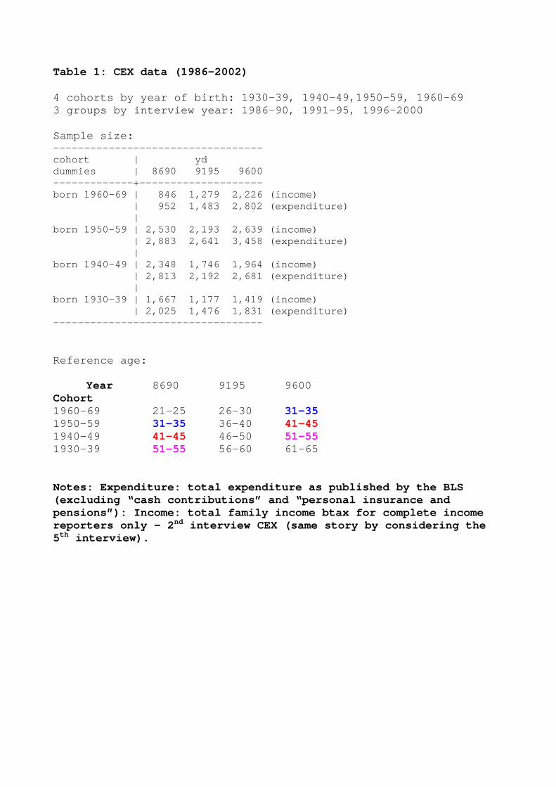
were obtained throughout by deflating using the Consumer Price Index. Table 1 provides

some sample summary statistics, including the cohort definitions and subsample sizes.

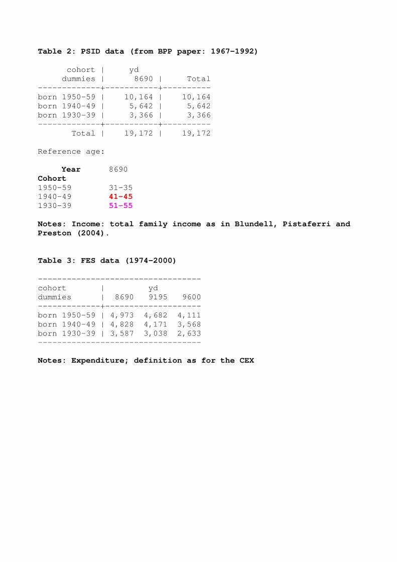
We complemented information from the CEX with information from the Panel Study of

Income Dynamics (PSID) and from the British Family Expenditure Survey (FES) for the

United Kingdom. Unlike the CEX, the PSID collects longitudinal annual data on a sample of

households followed on a consistent basis since 1968. We examine family disposable income

in the PSID for a sample of couples with and without children as described in Blundell,

Pistaferri and Preston (2004, 2005). The UK FES contains both detailed household income

and consumption data within the same survey, though total expenditures are only recorded

for a few weeks, and so may suffer from measurement errors due to problems like infrequency

of purchase.

For all surveys, for stability we focus on a sample of married couples (with or without

children) and define cohorts based on the year of birth of the head, which we conventionally

take to be the husband. Tables 2 and 3 present the summary statistics for our PSID and

the FES samples, respectively. A caveat regarding these data is that there is likely to be

under reporting in both tails of the income and consumption distributions, because many

poor households (such as the homeless) will be excluded, and wealthy households are also

likely to be underreported, both because their incentive to fill out the lengthy surveys is low,

and because of data topcoding by the reporting agencies. This is one reason why we used

robust measures distribution moments as discussed earlier.

6 The Empirical Distributions of Consumption and In-come

The Euler equation and permanent income models of the previous sections are likely to be

oversimplifications of reality. Our goal here is to check if their theoretical distribution im-

9

plications are roughly consistent with empirical distributions of income and consumption

data, which would be the case if the models at least coarsely approximate the income and

consumption behavior of most households.

To assess empirically the distribution implications of these models, consider a cross-section

of individuals, all of the same age τ . By definition, τμ and σ2 are unconditional moments of

the distribution of consumption. If the individuals in the sample are sufficiently similar, in

the sense of having similar unconditional moments μ and σ2, then the model can be tested

by examining whether the shape of the distribution of cτ across individuals in the sample

is close to normal. These are unconditional moments for each individual, so these tests do

not rule out conditional differences or correlations. For example, shocks can be conditionally

heteroskedastic and correlated across individuals. Similarly, having μ and σ2 be the same

across consumers does not mean that every consumer has the same consumption or the same

permanent income on average, but rather that each individual’s age τ permanent income

or consumption is drawn from some common underlying unconditional distribution that is

characterized by these moments, where by ‘unconditional’ we mean not conditioning on the

individual’s previous consumption, income, or other attributes.

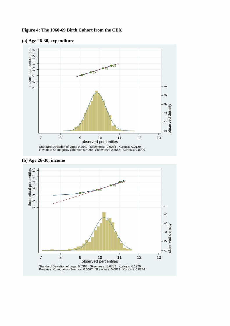
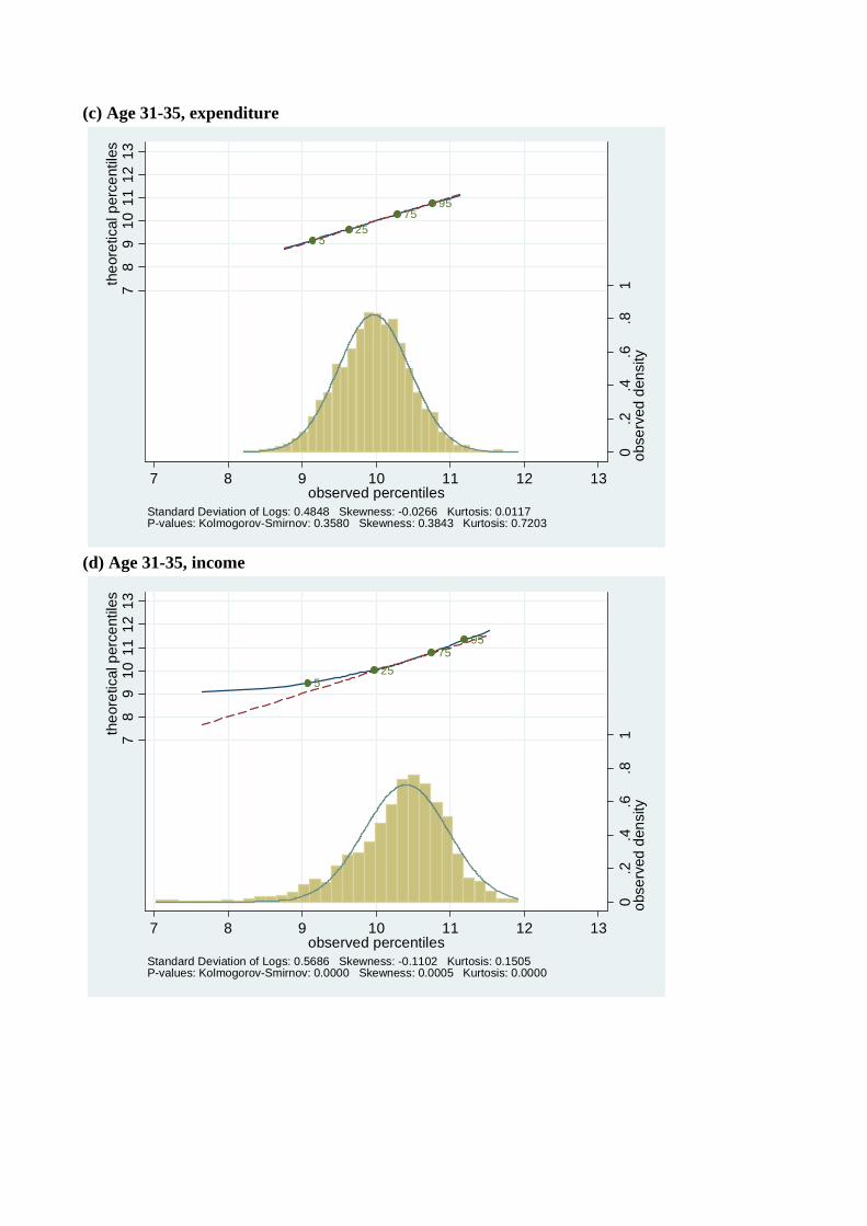
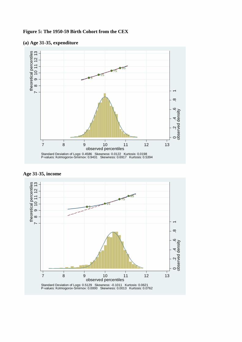
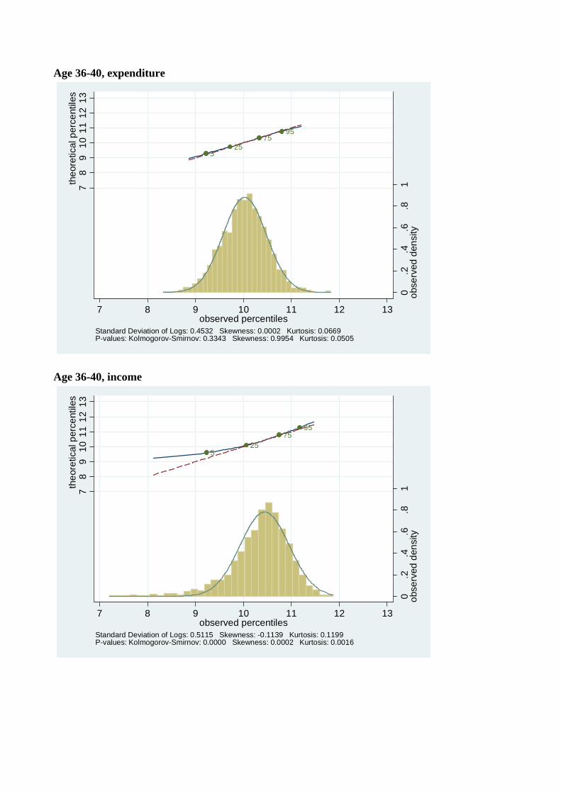
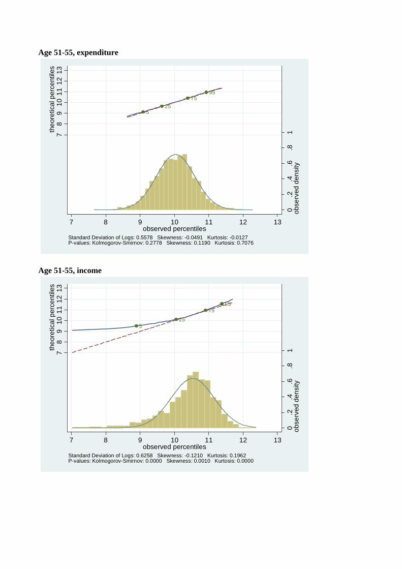
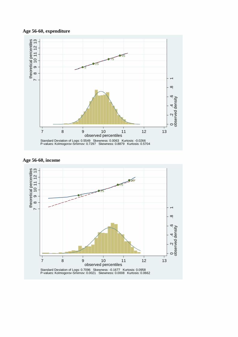
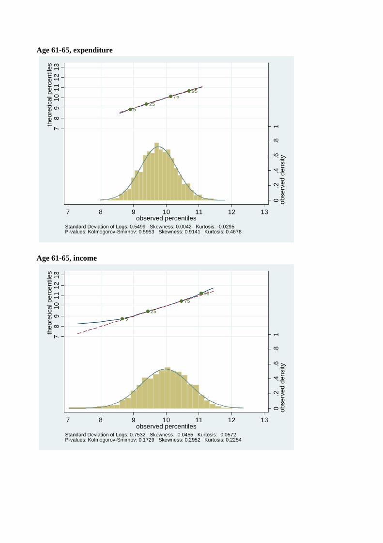
Figures 4-7 show the distribution of log expenditure and log income across the life-cycle for

each of four birth decade cohorts available from the Consumer Expenditure Surveys, beginning

with the youngest cohort (those born in the 1960’s). For each cohort, the distribution of log

consumption and log income is presented at each five year age interval in their lifecycle. So,

e.g., Figures 4(a) and 4(b) are consumption and income from the 1960’s cohort when they

were aged 26-30, Figures 4(c) and 4(d) are the same variables for the same cohort when they

are aged 31-35, Figure 5 has the same data for the 1970’s cohort going up to age 41-45, etc.,.

Figure 4(a) shows a log real expenditure distribution that is very close to normal. In

contrast, Figure 4(b) shows that log real income for these households is much further from

normal with the upper tail skewness that is typical of income distributions, and greater

kurtosis as well. A similar pattern holds across all age groups. These and the other log

income distributions we report also show a long lower tail. We expect that at least some of

this observed lower tail behavior is due to measurement error, e.g., there may be considerable

under reporting of income at these levels, and relatively small absolute errors in reported

10

income at low absolute levels of income may cause large distortions in the distribution of

income after taking logs.

Comparing people of the same ages across cohorts in Figures 4 to 7 shows that younger

cohorts have a higher dispersion of income and consumption, e.g., 31 to 35 year olds born

in the 1960’s have a higher variance of income than 31 to 35 year olds born in the 1970’s.

A similar pattern holds up across most age groups and cohorts. Also, in accordance with

Kalecki (1945) and Deaton and Paxson (1992), and consistent with Gibrat’s law, as every

birth cohort ages, their distributions of income and consumption become more dispersed.

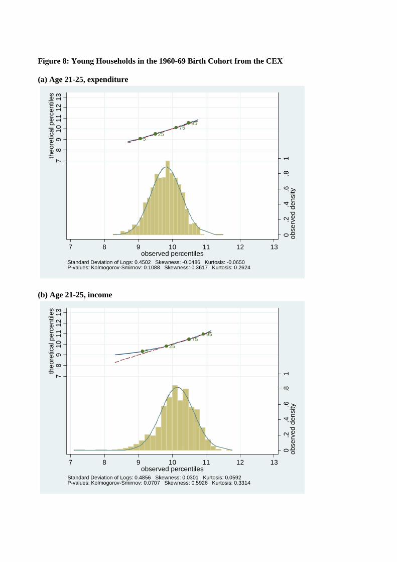
In Figure 8 we report data for the youngest available age group, which is 21-25 year olds

born in the 1960’s. Figure 8 shows that the distributions for these very young households are

further from log normal than for the older groups, which is again consistent with our theory of

distributions determined by Gibrat’s law. Above ages 25 or 30 departures from log normality

of consumption are very small and do not seem to systematically decrease further with age,

which suggests that by relatively early in one’s working life enough shocks have accumulated

to get close to asymptotic normality.

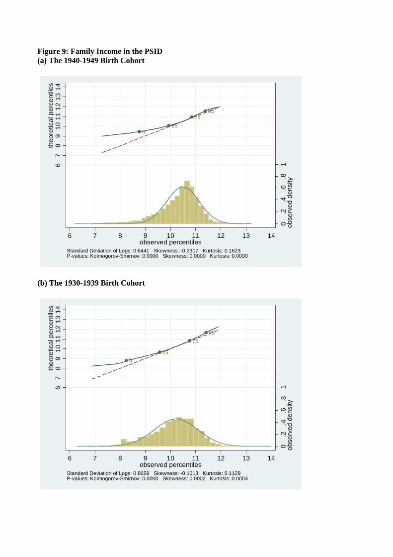
Our theory suggests that consumption should be closer to log normal than income, be-

cause income contains a potentially large transitory component in addition to a log normal

permanent income component. This is what we found in the CEX, but one might worry that

departures from log normality in CEX income data could be due measurement error, because

income may be measured less precisely than consumption in that data set. As a check, in

Figure 9 we examine income by birth cohort and age but this time for log family disposable

income from the PSID data set, which measures income more carefully than the CEX. We

find significant deviations from normality of log income in this data, similar to the departures

from log normality found in the CEX.

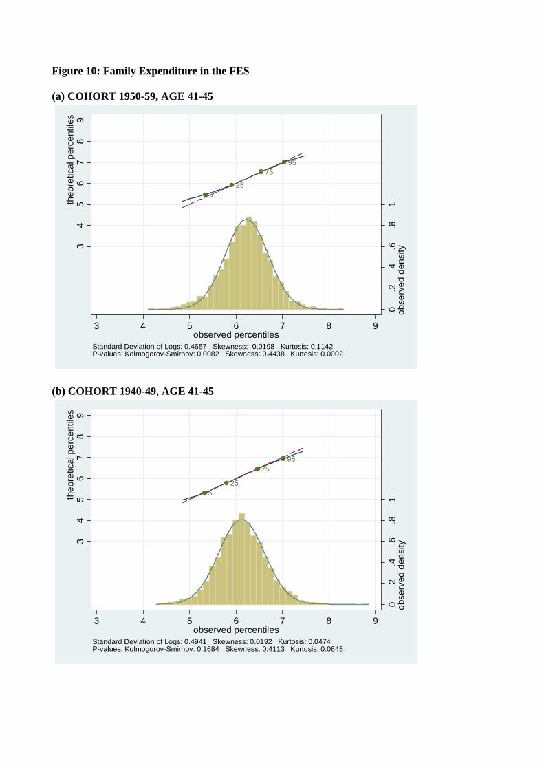
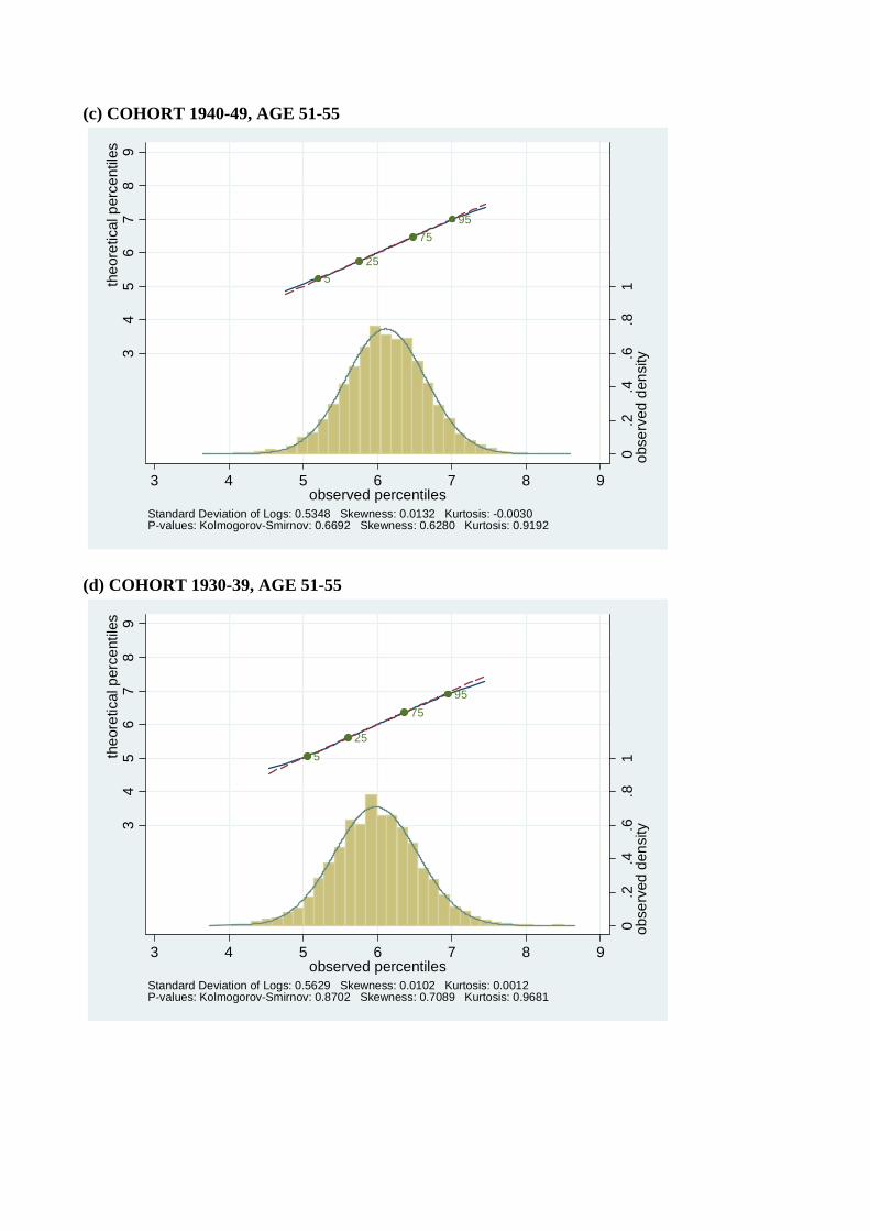
To show that the finding of normality of log consumption is not exclusive to the United

States, in Figure 10 we report consumption data by birth cohort and age from the British

FES. As in the CEX, consumption in the FES is very close to log normal.

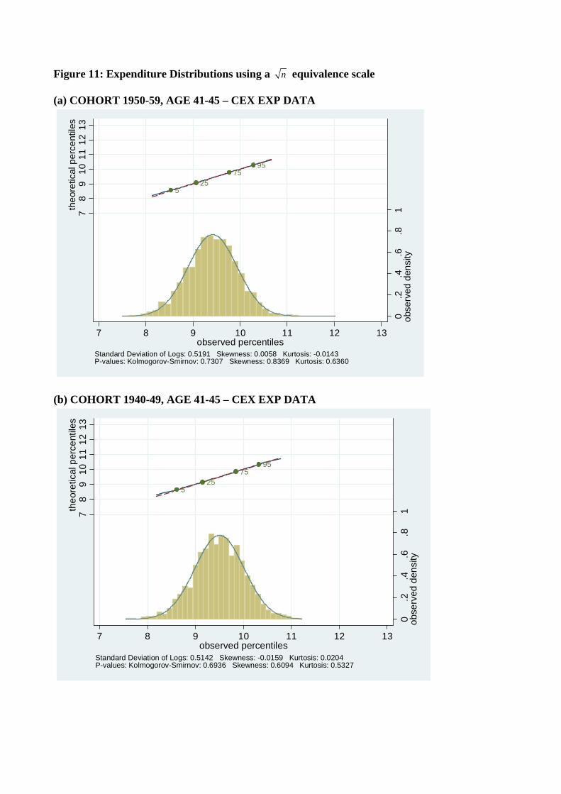
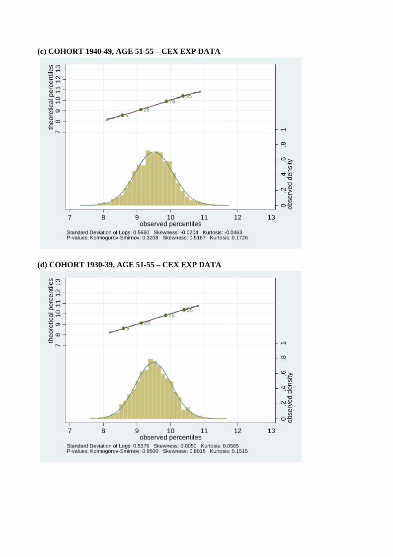
Our data includes households with varying numbers of children, because subpopulations

sorted by household size would not be comparable across age brackets. For example, house-

holds at age 40 with three children are more representative of the general population than

11

households at age 20 that have three children. However, numbers of children correlates with

income, and affects the propensity to consume out of current income. So as further check

on the robustness of our results, we recalculated distributions after dividing each household’s

income and consumption by√n where n is family size, thereby following a common practice

of using√n as an equivalence scale. These results, which remain consistent with our other

findings, are presented in Figure 11.

7 Conclusions

The income distribution has long been known to be approximately log normal. We have shown

that the consumption distribution is also close to log normal, and that within demographically

homogeneous groups, the distribution of consumption is much closer to log normal than is the

distribution of income. We also demonstrate that these empirical regularities are implications

of traditional models of the evolution of income and consumption, specifically, that the theory

which motivates Gibrat’s law should apply to permanent income and consumption (via Euler

equations), rather than to total income as originally formulated.

We would not expect perfect normality for a variety of reasons. Traditional permanent

income and Euler equation models are implausibly simplistic, so we should not expect them

to hold exactly. Also, the CLT is an asymptotic property while individuals only have finite

lifespans. Even when permanent income is close to log normal for some individuals, their

consumption may depart from log normality if marginal utility differs substantially from log

consumption, or if liquidity constraints, precautionary savings, or purchases of large durables

produce enough dependence in Euler equation innovations to violate the conditions required

for a CLT. More generally, normality may not hold for some individuals because their time

series of shocks may possess features such as bτ ’s far from one or long memory, that violate

the regularity conditions required for a CLT. Despite these possible problems, we find that

the observed distributions of consumption and income to be broadly consistent with the

distribution implications of these models, across cohorts, over time, and across data sets.

Other explanations for the observed consumption and income distributions may exist.

For example, if consumption is very badly measured, then its observed distribution could

be dominated by measurement errors that happen to be log normal. Another possibility is

12

based on the observation that higher income households tend to consume a smaller fraction

of income than lower income households, resulting in a consumption distribution that has

a thinner upper tail than the income distribution. If the income distribution is close to

log normal except for a thick (Pareto) upper tail, the consumption distribution should then

have a thinner upper tail, which could by coincidence be almost the same size as its lower

tail, resulting in a near normal distribution. These alternative explanations for consumption

log normality require coincidences that we find less plausible than our derivations based on

permanent income and Euler equation models, though these alternatives could be contributing

factors in the observed distributions.

As discussed in the introduction, the finding that Gibrat’s law applies to consumption

within cohorts has many important implications for welfare and inequality measurement,

aggregation, and econometric model analysis, and results in additional regularities in the dis-

tributions of related variables. It would be interesting to test if other economic variables that

are determined either by Euler equations or decompositions into permanent and transitory

components display a similar conformity to Gibrat’s law.

References

[1] Aitchison, J., and J.A.C. Brown (1957), The Lognormal Distribution, Cambridge Uni-versity Press, Cambridge.

[2] Banks, J. Blundell, R. and A. Lewbel (1997), ‘Quadratic Engel Curves, Indirect TaxReform and Welfare’, Review of Economics and Statistics, Vol. LXXIX, No.4, 527-539,November.

[3] Battistin, E. (2003), “Errors in Survey Reports of Consumption Expenditures”, WorkingPaper 07/03, Institute for Fiscal Studies, London.

[4] Blundell, R., L. Pistaferri and I. Preston (2004), “Imputing consumption in the PSIDusing food demand estimates from the CEX”, Institute for Fiscal Studies, WP04/27,(http://www.ifs.org.uk/ workingpapers/ wp0427.pdf).

[5] Blundell, R., L. Pistaferri and I. Preston (2005), “Consumption Inequality and PartialInsurance”, Consumption Inequality and Partial Insurance, (with L. Pistaferri and I.Preston), Institute for Fiscal Studies, WP04/27, revised May 2005.

[6] Blundell, R., and I. Preston (1995), ‘Income, Expenditure and the Living Standards ofUK Households’ Fiscal Studies, Vol. 16, No.3, 40-54, 1995.

13

[7] Blundell, R., and I. Preston (1998), “Consumption inequality and income uncertainty”,Quarterly Journal of Economics 113, 603-640.

[8] Deaton, A. (1992), Understanding Consumption. Baltimore: John Hopkins UniversityPress.

[9] Deaton, A., and C. Paxson (1994), “Intertemporal choice and inequality”, Journal ofPolitical Economy, 102, 384-94.

[10] Friedman, M. (1957), A Theory of the Consumption Function, Princeton: PrincetonUniversity Press.

[11] Gabaix, X. (1999) ‘Zipf’s Law for Cities: An Explanation’, The Quarterly Journal ofEconomics, vol. 113, no. 3 (August), pp. 739-767.

[12] Gibrat, R. (1931). Les Inegalites Economiques. Librairie du Recueil Sirey. Paris.

[13] Groeneveld, R.A. and Meeden, G. (1984), Measuring Skewness and Kurtosis, The Sta-tistician, Vol. 33, No. 4, 391-399.

[14] Hall, R. E. (1978), "Stochastic Implications of the Life Cycle-Permanent Income Hy-pothesis: Theory and Evidence," The Journal of Political Economy, 86, 971-987.

[15] Hampel, F.R., Ronchetti, E.M., Rousseeuw, P.J., and Stahel, W.A. (1986), Robust Sta-tistics, John Wiley and Sons: New York.

[16] Hinkley, D.V. (1975), On Power Transormations to Simmetry, Biometrika, Vol. 62, No.1, 101-111.

[17] Kalecki, M. (1945), "On the Gibrat Distribution," Econometrica, 13, 161-170.

[18] MaCurdy, T. E. (1982), "The use of time series processes to model the error structure ofearnings in a longitudinal data analysis," Journal of Econometrics, 18, 83-114.

[19] Meghir, C., and L. Pistaferri (2004), “Income variance dynamics and heterogeneity”,Econometrica, 72(1), 1-32.

[20] Meyer, B. and J. Sullivan (2003), “Measuring the Well-Being of the Poor Using Incomeand Consumption’, Journal of Human Resources, 1180-220.

[21] Moors, J.J.A. (1988), A Quantile Alternative to Kurtosis, The Statistician, Vol. 37, No.1, 25-32.

[22] Wooldridge, J. M. and H White, (1988), "Some Invariance Principles and Central LimitTheorems for Dependent Heterogeneous Processes," Econometric Theory, 4, 210-230.

[23] Zipf, G.K. (1949), Human Behavior and the Principle of Least Effort, Addison-Wesley.

14

Figure 1: The Distribution of Log Household Income in the US

525

7595

0.2

.4.6

.81

obse

rved

den

sity

78

910

1112

13th

eore

tical

per

cent

iles

7 8 9 10 11 12 13observed percentiles

Standard Deviation of Logs: 0.5686 Skewness: -0.1102 Kurtosis: 0.1505P-values: Kolmogorov-Smirnov: 0.0000 Skewness: 0.0005 Kurtosis: 0.0000

Notes: Age 31-35, income Figure 2: The Distribution of Log Household Consumption in the US

525

7595

0.2

.4.6

.81

obse

rved

den

sity

78

910

1112

13th

eore

tical

per

cent

iles



Notes: Age 31-35, expenditure

Figure 3: Consumption in the UK

525

7595

0.2

.4.6

.81

obse

rved

den

sity3

45

67

89

theo

retic

al p

erce

ntile

s


Standard Deviation of Logs: 0.5629 Skewness: 0.0102 Kurtosis: 0.0012P-values: Kolmogorov-Smirnov: 0.8702 Skewness: 0.7089 Kurtosis: 0.9681

Notes: FES EXP DATA: COHORT 1930-39, AGE 51-55

Table 1: CEX data (1986-2002) 4 cohorts by year of birth: 1930-39, 1940-49,1950-59, 1960-69 3 groups by interview year: 1986-90, 1991-95, 1996-2000 Sample size: ---------------------------------- cohort | yd dummies | 8690 9195 9600 -------------+-------------------- born 1960-69 | 846 1,279 2,226 (income) | 952 1,483 2,802 (expenditure) | born 1950-59 | 2,530 2,193 2,639 (income) | 2,883 2,641 3,458 (expenditure) | born 1940-49 | 2,348 1,746 1,964 (income) | 2,813 2,192 2,681 (expenditure) | born 1930-39 | 1,667 1,177 1,419 (income) | 2,025 1,476 1,831 (expenditure) ---------------------------------- Reference age:

Year 8690 9195 9600 Cohort 1960-69 21-25 26-30 31-35 1950-59 31-35 36-40 41-45 1940-49 41-45 46-50 51-55 1930-39 51-55 56-60 61-65 Notes: Expenditure: total expenditure as published by the BLS (excluding “cash contributions” and “personal insurance and pensions”): Income: total family income btax for complete income reporters only - 2nd interview CEX (same story by considering the 5th interview).

Table 2: PSID data (from BPP paper: 1967-1992) cohort | yd dummies | 8690 | Total -------------+-----------+---------- born 1950-59 | 10,164 | 10,164 born 1940-49 | 5,642 | 5,642 born 1930-39 | 3,366 | 3,366 -------------+-----------+---------- Total | 19,172 | 19,172 Reference age:

Year 8690 Cohort 1950-59 31-35 1940-49 41-45 1930-39 51-55

Notes: Income: total family income as in Blundell, Pistaferri and Preston (2004). Table 3: FES data (1974-2000) ---------------------------------- cohort | yd dummies | 8690 9195 9600 -------------+-------------------- born 1950-59 | 4,973 4,682 4,111 born 1940-49 | 4,828 4,171 3,568 born 1930-39 | 3,587 3,038 2,633 ---------------------------------- Notes: Expenditure; definition as for the CEX

Figure 4: The 1960-69 Birth Cohort from the CEX (a) Age 26-30, expenditure

525

7595

0.2

.4.6

.81

obse

rved

den

sity

78

910

1112

13th

eore

tical

per

cent

iles



(b) Age 26-30, income

525

7595

0.2

.4.6

.81

obse

rved

den

sity

78

910

1112

13th

eore

tical

per

cent

iles



(c) Age 31-35, expenditure

525

7595

0.2

.4.6

.81

obse

rved

den

sity

78

910

1112

13th

eore

tical

per

cent

iles



(d) Age 31-35, income

525

7595

0.2

.4.6

.81

obse

rved

den

sity

78

910

1112

13th

eore

tical

per

cent

iles



Figure 5: The 1950-59 Birth Cohort from the CEX (a) Age 31-35, expenditure

525

7595

0.2

.4.6

.81

obse

rved

den

sity

78

910

1112

13th

eore

tical

per

cent

iles



Age 31-35, income

525

7595

0.2

.4.6

.81

obse

rved

den

sity

78

910

1112

13th

eore

tical

per

cent

iles



Age 36-40, expenditure

525

7595

0.2

.4.6

.81

obse

rved

den

sity

78

910

1112

13th

eore

tical

per

cent

iles



Age 36-40, income

525

7595

0.2

.4.6

.81

obse

rved

den

sity

78

910

1112

13th

eore

tical

per

cent

iles




525

7595

0.2

.4.6

.81

obse

rved

den

sity

78

910

1112

13th

eore

tical

per

cent

iles



Age 41-45, income

525

7595

0.2

.4.6

.81

obse

rved

den

sity

78

910

1112

13th

eore

tical

per

cent

iles



Figure 6: The 1940-49 Birth Cohort from the CEX Age 41-45, expenditure

525

7595

0.2

.4.6

.81

obse

rved

den

sity

78

910

1112

13th

eore

tical

per

cent

iles


Standard Deviation of Logs: 0.4980 Skewness: -0.0081 Kurtosis: -0.0205P-values: Kolmogorov-Smirnov: 0.7181 Skewness: 0.7931 Kurtosis: 0.5307

Age 41-45, income

525

7595

0.2

.4.6

.81

obse

rved

den

sity

78

910

1112

13th

eore

tical

per

cent

iles




525

7595

0.2

.4.6

.81

obse

rved

den

sity

78

910

1112

13th

eore

tical

per

cent

iles



Age 46-50, income

525

7595

0.2

.4.6

.81

obse

rved

den

sity

78

910

1112

13th

eore

tical

per

cent

iles




525

7595

0.2

.4.6

.81

obse

rved

den

sity

78

910

1112

13th

eore

tical

per

cent

iles



Age 51-55, income

525

7595

0.2

.4.6

.81

obse

rved

den

sity

78

910

1112

13th

eore

tical

per

cent

iles



Figure 7: The 1930-39 Birth Cohort from the CEX Age 51-55, expenditure

525

7595

0.2

.4.6

.81

obse

rved

den

sity

78

910

1112

13th

eore

tical

per

cent

iles



Age 51-55, income

525

7595

0.2

.4.6

.81

obse

rved

den

sity

78

910

1112

13th

eore

tical

per

cent

iles




525

7595

0.2

.4.6

.81

obse

rved

den

sity

78

910

1112

13th

eore

tical

per

cent

iles


Standard Deviation of Logs: 0.5549 Skewness: 0.0063 Kurtosis: -0.0266P-values: Kolmogorov-Smirnov: 0.7297 Skewness: 0.8879 Kurtosis: 0.5704

Age 56-60, income

525

7595

0.2

.4.6

.81

obse

rved

den

sity

78

910

1112

13th

eore

tical

per

cent

iles




525

7595

0.2

.4.6

.81

obse

rved

den

sity

78

910

1112

13th

eore

tical

per

cent

iles



Age 61-65, income

525

7595

0.2

.4.6

.81

obse

rved

den

sity

78

910

1112

13th

eore

tical

per

cent

iles



Figure 8: Young Households in the 1960-69 Birth Cohort from the CEX (a) Age 21-25, expenditure

525

7595

0.2

.4.6

.81

obse

rved

den

sity

78

910

1112

13th

eore

tical

per

cent

iles



(b) Age 21-25, income

525

7595

0.2

.4.6

.81

obse

rved

den

sity

78

910

1112

13th

eore

tical

per

cent

iles



Figure 9: Family Income in the PSID (a) The 1940-1949 Birth Cohort

525

7595

0.2

.4.6

.81

obse

rved

den

sity

67

89

1011

1213

14th

eore

tical

per

cent

iles

6 7 8 9 10 11 12 13 14observed percentiles


(b) The 1930-1939 Birth Cohort

525

7595

0.2

.4.6

.81

obse

rved

den

sity

67

89

1011

1213

14th

eore

tical

per

cent

iles

6 7 8 9 10 11 12 13 14observed percentiles


Figure 10: Family Expenditure in the FES (a) COHORT 1950-59, AGE 41-45

525

7595

0.2

.4.6

.81

obse

rved

den

sity3

45

67

89

theo

retic

al p

erce

ntile

s



(b) COHORT 1940-49, AGE 41-45

525

7595

0.2

.4.6

.81

obse

rved

den

sity3

45

67

89

theo

retic

al p

erce

ntile

s



(c) COHORT 1940-49, AGE 51-55

525

7595

0.2

.4.6

.81

obse

rved

den

sity3

45

67

89

theo

retic

al p

erce

ntile

s



(d) COHORT 1930-39, AGE 51-55

525

7595

0.2

.4.6

.81

obse

rved

den

sity3

45

67

89

theo

retic

al p

erce

ntile

s



Figure 11: Expenditure Distributions using a n equivalence scale (a) COHORT 1950-59, AGE 41-45 – CEX EXP DATA

525

7595

0.2

.4.6

.81

obse

rved

den

sity

78

910

1112

13th

eore

tical

per

cent

iles



(b) COHORT 1940-49, AGE 41-45 – CEX EXP DATA

525

7595

0.2

.4.6

.81

obse

rved

den

sity

78

910

1112

13th

eore

tical

per

cent

iles



(c) COHORT 1940-49, AGE 51-55 – CEX EXP DATA

525

7595

0.2

.4.6

.81

obse

rved

den

sity

78

910

1112

13th

eore

tical

per

cent

iles



(d) COHORT 1930-39, AGE 51-55 – CEX EXP DATA

525

7595

0.2

.4.6

.81

obse

rved

den

sity

78

910

1112

13th

eore

tical

per

cent

iles



Date post:	12-May-2019
Category:	Documents
Upload:	buinhu
View:	217 times
Download:	0 times

Why is Consumption More Log Normal Than Income? Gibrat’s ... · Why is Consumption More Log...

Documents