Why seismic-to-well ties are difficult - CREWES · Why seismic-to-well ties are difficult Gary F....

Why well tying is difficult

CREWES Research Report — Volume 25 (2013) 1

Why seismic-to-well ties are difficult

Gary F. Margrave

SUMMARY

Tying seismic data to well control is a crucial step in seismic inversion and interpretation. This is where key ambiguities that prevent the interpretation of a seismic image as bandlimited reflectivity are resolved. Reflectivity can be calculated directly from suitable well logs while the estimation of reflectivity from seismic data requires the unambiguous determination of the seismic wavelet and the removal of the same. However, due to the unavoidable presence of anelastic attenuation, the very notion of a single seismic wavelet is not robust. Instead, constant-Q theory predicts that the source waveform evolves continuously as it propagates in the subsurface. It progressively loses frequency content and undergoes continual phase changes. This evolution means that each reflecting structure in the subsurface is illuminated by a unique waveform. The use of stationary (standard) deconvolution methods leads to a trace with unbalanced amplitude, in both time and frequency, and time-variant residual phase. Attempts to remedy this by time-variant balancing leads to a trace that can, at best, be tied to a well in a local time zone but which has misties above and below that zone. Nonstationary deconvolution or inverse Q filtering can potentially address these effects but the former relies on a statistical reflectivity model while the latter requires knowledge of Q. The theoretical advantage of inverse Q filtering over nonstationary deconvolution largely vanishes with the presence of even small noise levels. Processes that successfully address nonstationarity must also be data adaptive to successfully deal with noise. Well tying can be improved by using deconvolution algorithms and well-tying methodologies that are consistent with constant-Q theory.

INTRODUCTION

Tying seismic data to wells is meant to ensure that that the seismic data lives up to its promise of being a robust estimate of bandlimited reflectivity. Reflectivity can be calculated directly in a well from suitable well logs (usually sonic and density logs) so well tying seeks to use the well information to “calibrate” the seismic estimate. Since data processing is designed to estimate reflectivity, one might hope that well-tying would happen automatically with modern algorithms. However, this is not generally observed to be the case and it is the thesis of this paper that failure to adequately address anelastic attenuation is a first-order culprit. The commonly assumed convolutional model, which is the basis for most seismic deconvolution algorithms, is invalidated by the presence of attenuation. No matter the physical mechanism for attenuation, or whether it is intrinsic or extrinsic, as long as the attenuation is both time and frequency dependent then the convolutional model is not valid. This is because the wavelet evolves as it propagates, progressively losing high frequencies and undergoing phase rotations. The convolutional model assumes translational invariance meaning that the wavelet does not evolve and that an identical wavelet is incident on all reflectors. Data processing has recognized this in limited ways that are adequate for zone-of-interest interpretation but cause problems for larger scale inversions. For example, it can be argued that in a sufficiently limited time zone the convolutional model is approximately valid, and that deconvolution can

Margrave

2 CREWES Research Report — Volume 25 (2013)

estimate a reasonable wavelet. However, it will be shown here that above and below that design window the deconvolution becomes increasingly erroneous. Similar arguments hold for the wavelet estimations made during well tying. At best they are valid locally and become increasingly erroneous with increasing displacement from the analysis window.

Methods used for well tying vary but often follow empirical rules and techniques. White (1980) gives a spectral coherence matching formula for the estimation of a matching wavelet. While theoretically valid if the convolutional model is assumed, more approximate approaches are common. Usually a 1D synthetic seismogram is constructed from the well information but the well logs may first be altered by “stretching and squeezing”. The synthetic seismogram is normally a simple convolutional one where the wavelet amplitude spectrum is that required to match the seismic data (i.e. the amplitude spectrum of the seismic divided by that of the well reflectivity) and the phase is initially zero. Then a “phase rotation” is determined by scanning through all possible constant phase rotations to find that which minimizes the L2 norm of the difference between a seismic trace at the well and the synthetic. Usually this process is done in a very limited time window dictated by the length of available logs.

Possible objections to the standard process are many, including (1) the log information may be of doubtful quality or the 6 inch borehole measurements may not represent the wider stratigraphy, (2) the available well logs may be very short, (3) matching is usually done to primary reflectivity and there may be multiples present in the seismic data, (4) the sonic log may have been through an interpretive stretch-squeeze process, (5) simple phase scanning may be insufficient to model the actual wavelet, (6) when multiple wells are available, different wavelets are often obtained from each, (7) the character tie between synthetic and data may be ambiguous (especially a problem with long logs) (8) the extracted wavelet may have doubtful validity above and below the estimation window (due to attenuation). This report will mainly be concerned with the last point.

A PERFECT CASE WITH DOUBTFUL PHYSICAL VALIDITY

As mentioned previously, the convolutional model is the basis for the most common deconvolution algorithms as well as most well-tie procedures, so this is an appropriate place to start. As used in practice, the convolutional mode posits a relationship between the reflectivity function ( )r t , the seismic wavelet ( )w t , and the seismic trace ( )s t of

the form

( ) ( ) ( ) ( )s t w t r t n t= • + (1)

where ( )n t is noise. Strictly speaking, this is not derivable from the wave equation,

rather, Green’s theorem says

( ) ( ) ( ) ( )s t w t I t n t= • + (2)

where ( )I t is the earth’s impulse response. The difference between ( )I t and ( )r t is

very significant for this discussion. The former is the full response of the earth system to



an impulsive source and includes all physical effects of wave propagation such as wavefront spreading, reflection, transmission, multiples, attenuation, and anything else conceivable. On the other hand, ( )r t is simply a time series whose amplitudes represent

the reflection coefficients of subsurface structures. In order to assert that equation 1 models a seismic trace, we must claim that data processing has corrected for all of these physical effects and somehow converted ( )I t into ( )r t . This is a tall order and is

almost certainly achieved with considerable uncertainty.

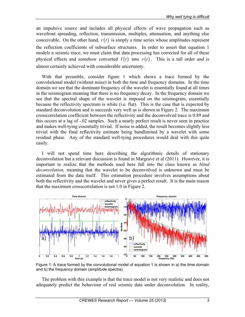
With that preamble, consider figure 1 which shows a trace formed by the convolutional model (without noise) in both the time and frequency domains. In the time domain we see that the dominant frequency of the wavelet is essentially found at all times in the seismogram meaning that there is no frequency decay. In the frequency domain we see that the spectral shape of the wavelet is imposed on the seismogram, essentially because the reflectivity spectrum is white (i.e. flat). This is the case that is expected by standard deconvolution and is succeeds very well as is shown in Figure 2. The maximum crosscorrelation coefficient between the reflectivity and the deconvolved trace is 0.89 and this occurs at a lag of -.02 samples. Such a nearly perfect result is never seen in practice and makes well-tying essentially trivial. If noise is added, the result becomes slightly less trivial with the final reflectivity estimate being bandlimited by a wavelet with some residual phase. Any of the standard well-tying procedures would deal with this quite easily.

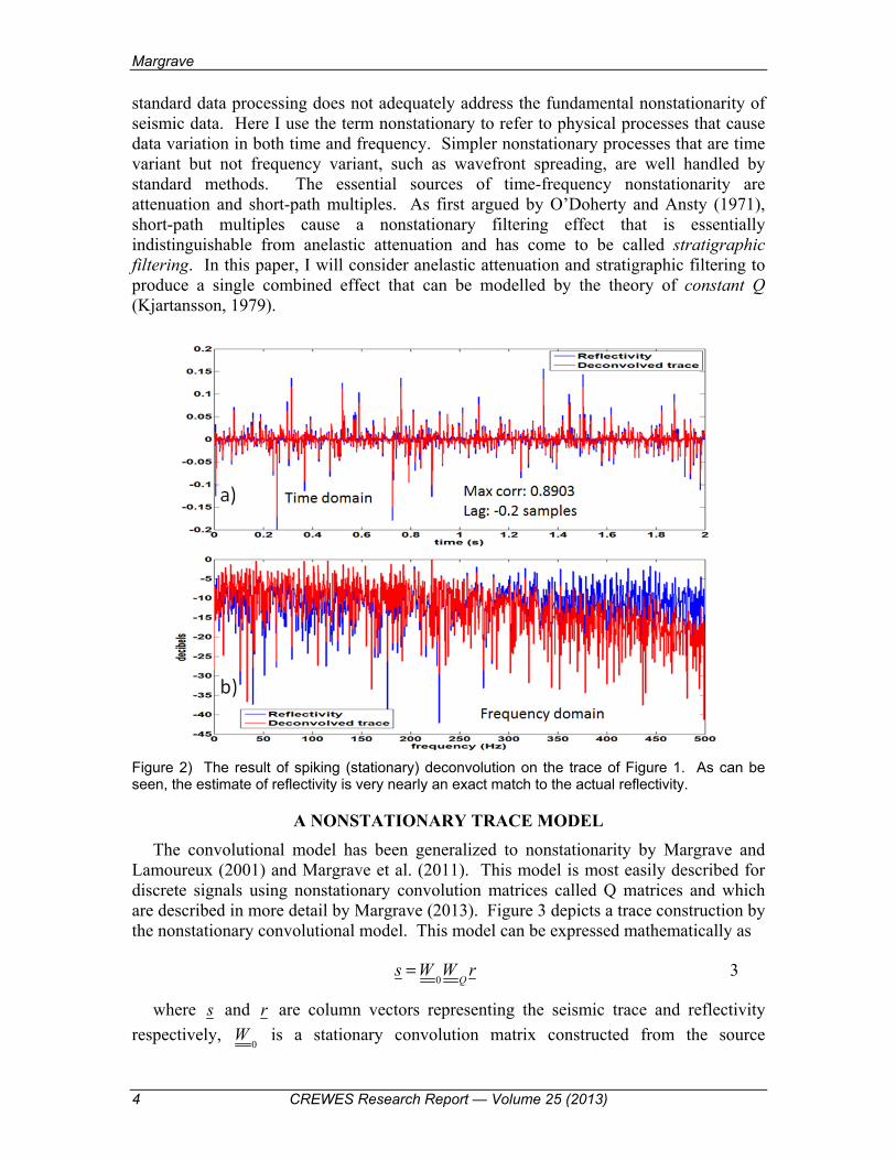
I will not spend time here describing the algorithmic details of stationary deconvolution but a relevant discussion is found in Margrave et al (2011). However, it is important to realize that the methods used here fall into the class known as blind deconvolution, meaning that the wavelet to be deconvolved is unknown and must be estimated from the data itself. This estimation procedure involves assumptions about both the reflectivity and the wavelet and never gives a perfect result. It is the main reason that the maximum crosscorrelation is not 1.0 in Figure 2.

Figure 1: A trace formed by the convolutional model of equation 1 is shown in a) the time domain and b) the frequency domain (amplitude spectra).

The problem with this example is that the trace model is not very realistic and does not adequately predict the behaviour of real seismic data under deconvolution. In reality,

Margrave


standard data processing does not adequately address the fundamental nonstationarity of seismic data. Here I use the term nonstationary to refer to physical processes that cause data variation in both time and frequency. Simpler nonstationary processes that are time variant but not frequency variant, such as wavefront spreading, are well handled by standard methods. The essential sources of time-frequency nonstationarity are attenuation and short-path multiples. As first argued by O’Doherty and Ansty (1971), short-path multiples cause a nonstationary filtering effect that is essentially indistinguishable from anelastic attenuation and has come to be called stratigraphic filtering. In this paper, I will consider anelastic attenuation and stratigraphic filtering to produce a single combined effect that can be modelled by the theory of constant Q (Kjartansson, 1979).

Figure 2) The result of spiking (stationary) deconvolution on the trace of Figure 1. As can be seen, the estimate of reflectivity is very nearly an exact match to the actual reflectivity.

A NONSTATIONARY TRACE MODEL

The convolutional model has been generalized to nonstationarity by Margrave and Lamoureux (2001) and Margrave et al. (2011). This model is most easily described for discrete signals using nonstationary convolution matrices called Q matrices and which are described in more detail by Margrave (2013). Figure 3 depicts a trace construction by the nonstationary convolutional model. This model can be expressed mathematically as

0 Q

s W W r= 3

where s and r are column vectors representing the seismic trace and reflectivity

respectively, 0

W is a stationary convolution matrix constructed from the source



signature, 0w , and Q

W is a nonstationary convolution matrix that applies the constant-Q

impulse response. Q

W is called the Q matrix while 0

W is the source convolution matrix.

Each column of Q

W contains the impulse response of the constant-Q process for the

particular traveltime of the column. Figure 3 only shows the matrix product 0 Q

W W

while Figure 4 shows the individual matrices. It is apparent that 0

W has the Toeplitz

symmetry (or translation invariance) that is so essential in the convolutional model. This symmetry is destroyed by

QW which describes the time-frequency decay of the Q

process.

The traces resulting from the stationary trace model of equation 1 and the nonstationary model of equation 3 are compared in Figure 5. Since the source wavelet and the reflectivity were identical for this construction, all the differences are caused by the Q matrix. At early times, the effects of nonstationarity are not large but they build progressively as time increases. The loss of both amplitude and frequency content is clearly apparent such that the traces are very different at later times. Here the stationary and nonstationary models agree at early times. However, it is possible to build a convolutional model that agrees with the nonstationary model in any small time window but they will disagree dramatically outside this window.

Figure 3: Depiction of the nonstationary convolutional model of equation 3. The matrix product

0 QW W is shown as a single matrix here and as individual matrices in Figure 4.

Margrave


Figure 4: The individual matrices that compose the product

0 QW W in the nonstationary

convolutional model of equation 3. 0

W is a stationary (Toeplitz symmetric) matrix while Q

W

defines the time-frequency attenuation inherent in the Constant-Q process.

Figure 5: Comparisons of the traces for the stationary trace model of equation 1 and the nonstationary model of equation 3. The source wavelet and reflectivity are identical for both

models so that the Q matrix Q

W is entirely responsible for the differences.

Matrix multiplication is not generally commutative which means that 0 Q

W W cannot

be expected to equal 0Q

W W . This seems unfortunate because, given knowledge of Q,

we would like to process the nonstationary trace in such a way as to render it stationary



without yet knowing the source signature. The result could then be input to stationary deconvolution with a reasonable expectation of success. This means that we would like s defined by

1 1

0Q Q Qs W s W W W r− −= = 4

to be similar to 0stats W r= , the stationary trace. This could only happen if

0 QW W are

approximately commutative. A numerical experiment is shown in Figure 6 that suggests that this is true.

Figure 6: A numerical demonstration that

0 QW W (green trace) is almost equal to

0QW W (red

trace). Thus we expect that the application of an inverse Q matrix should render the nonstationary trace stationary.

WAVELET EVOLUTION DUE TO Q

The constant-Q theory of Kjartansson (1979) offers a first-order explanation of the evolution of a wavelet in an attenuating medium. Here “first-order” means that transmission effects are reasonably well described but reflection is ignored. This theory captures the wavelet decay with both time and frequency and the associated minimum-phase shifts. According to the constant Q theory, the amplitude spectrum of the wavelet evolves according to

Margrave


( ) ( ) /0ˆ ˆ, f t Qw f t w f e π−= 5

where ( )ˆ ,w f t is the amplitude spectrum after traveltime t, ( )0w f is the initial

amplitude spectrum (as emitted by the source), f is frequency, and Q is a rock property independent of frequency although time dependence is allowed. As first argued by Futterman (1962) and illustrated very well by Aki and Richards (2002), causality arguments completely determine the phase associated with the amplitude attenuation in equation 5. Both references show that the phase is determined by the minimum-phase condition that the Hilbert transform of the log-amplitude give the phase. Kjartannson (1979) gives the complete formula

( ) ( ) ( ) ( )0/ , ,0ˆ ˆ, f x v Q i f x Qw f x w f e π ϕ− −= 6

where x is distance travelled, 0v is a high-frequency reference velocity measured at

frequency 0f , and

( ) ( ), , 2 /f t Q f x v fϕ π= . 7

with ( )v f being the frequency dependent phase velocity given by

( ) 00

11 ln

fv f vQ fπ

= +

. 8

Defining traveltime 0/t x v= we can re-write equation 6 as

( ) ( ) 0

1/ 2 1 ln

0ˆ ˆ,ff t Q i f t

Q fw f t w f eπ π

π

− − − ≈ . 9

(These formulae are all written for positive f only and case must be taken when generalizing to negative frequencies.) Figure 7 shows the result of equation 9 when used to calculate the impulse response of the Q theory (corresponding to ( )0ˆ 1w f = ) and the

bandlimited response (corresponding to ( )0w f representing a minimum phase wavelet

with a dominant frequency of 100 Hz.). (See Margrave (2013) for a description of the software used to make this and similar figures.) The main thing to observe here is that there is no single “wavelet” that can be analyzed and perhaps deconvolved. Instead, there is a different wavelet for every possible traveltime (or travel distance) and so the seismic trace must have a continuously varying wavelet embedded in it. This continuous variation is encoded in the Q matrix of Figures 3 and 4 and is transferred to the seismogram in Figure 5. What we can say about these wavelets is that they are all derived from an initial source wavelet by the application of a minimum-phase forward Q filter. If the initial source wavelet is minimum phase, then so are all of the embedded wavelets.



As a second thought experiment, suppose we have a reflectivity consisting of a sequence of unit spikes placed every 0.2 s. Then applying

QW to this spike sequence

extracts the expected Q-impulse response every 0.2 s. Similarly, applying 0 Q

W W , to the

spike sequence extracts the evolution of an initial wavelet represented by 0

W . This is

shown in Figure 8.

Figure 7: a,b) The evolution of an initial impulse (Dirac Delta) in a constant-Q medium. Panel a) shows the wavelets in true relative size for various distances. Panel b) shows the wavelets after amplitude normalization and with most of the propagation delay removed. c,d) Similar to a,b) except thet the intial pulse was a bandlimited minimum phase wavelet.

Figure 8: A sequence of spikes representing a reflectivity (blue) is show after multiplication by

QW (green) and by

0 QW W (red) where

0W was a minimum phase, 20 Hz dominant, wavelet.

Margrave


In Figure 8, we observe that the bandlimited evolving wavelets always lag behind the corresponding unit spike by a progressively increasing amount. This lag time in controlled by the 0f parameter in equation 9. In generating Figure 8, 0f was taken to be

the Nyquist frequency of the simulation which was 500 Hz. Since 0f corresponds to the

frequency of measurement of velocity information, a better value for this would be the dominant frequency of well-logging which is about 12500 Hz. Figure 9 compares the result of using Q matrices with 0 500f = and with 0 12500f = Hz. As can be seen, the

delay of the wavelet behind the spike is much larger for 0 12500f = Hz. This happens

because 0f is the frequency at which the reference velocity 0v is assumed specified and

the spikes are at times defined by 0 0t xv= (see equations 6-9). Because the wavelet has a

dominant frequency near 20sf = Hz, it has a traveltime of ( )s st xv f= . The time

difference 0dr st t t= − is called the drift time and is always positive. The implication is

that a synthetic seismogram computed with the velocities measured by a sonic tool will predict event times that are too early by drt . This phenomenon can be corrected for in a

variety of ways including (1) calibrating the sonic velocities by using a check-shot survey, (2) given a Q estimate, we can calculate the expected well velocities at seismic frequencies using equation 8, (3) the seismogram can be constructed at the measured logging velocities and then stretched to seismic time by calculating the drift correction, (4) the sonic log can be interpretively stretched by moving key markers to greater depths until the synthetic seismogram appears to match. All of these methods are used in practice although (2) might have a theoretical preference.

Figure 9: Similar to Figure 8 except that the wavelet evolution for two different reference frequencies is compared. The reference frequency of 12500 Hz is roughly the dominant frequency of well-logging.

SYNTHETIC SEISMOGRAMS CREATED FROM REAL WELL LOGS

Before examining the performance of stationary deconvolution on a nonstationary synthetic, it is advisable to make a more realistic synthetic seismogram than that shown in Figure 1. That result was created from a synthetic reflectivity which fits the “white”



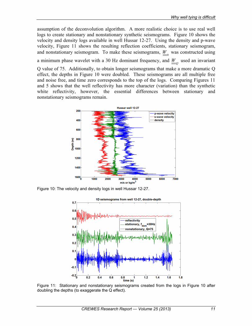
assumption of the deconvolution algorithm. A more realistic choice is to use real well logs to create stationary and nonstationary synthetic seismograms. Figure 10 shows the velocity and density logs available in well Hussar 12-27. Using the density and p-wave velocity, Figure 11 shows the resulting reflection coefficients, stationary seismogram, and nonstationary seismogram. To make these seismograms,

0W was constructed using

a minimum phase wavelet with a 30 Hz dominant frequency, and Q

W used an invariant

Q value of 75. Additionally, to obtain longer seismograms that make a more dramatic Q effect, the depths in Figure 10 were doubled. These seismograms are all multiple free and noise free, and time zero corresponds to the top of the logs. Comparing Figures 11 and 5 shows that the well reflectivity has more character (variation) than the synthetic white reflectivity, however, the essential differences between stationary and nonstationary seismograms remain.

Figure 10: The velocity and density logs in well Hussar 12-27.

Figure 11: Stationary and nonstationary seismograms created from the logs in Figure 10 after doubling the depths (to exaggerate the Q effect).

Margrave


STATIONARY DECONVOLUTION ON A NONSTATIONARY SEISMOGRAM

The performance of stationary deconvolution on the seismograms of Figure 11 is a good proxy for what happens when gain corrected, high quality, real seismic data is deconvolved. Gain correction is used to remove nonstationary effects that are frequency independent (like wavefront spreading) and by “high quality” it is meant that we are not considering any noise effects either random or coherent.

Both the stationary and nonstationary seismograms have a reflectivity that is not white. As shown in Figure 12, well log reflectivity has a flat “white” spectrum at high frequencies but at lower frequencies has a distinct spectral roll off. This is contrary to the assumptions of stationary deconvolution but causes relatively subtle low-frequency errors. Of greater interest and effect is the time and frequency variant spectrum of the nonstationary seismogram. While this “brute fact” is usually understood by data processors, its full range of consequences is not. The usual accommodation to spectral nonstationarity is to select a design window taken over the zone of interest and small enough that wavelet evolution should be small and within which the deconvolution operator is designed. For this purpose, I will use the time window 0.6 1.2t≤ ≤ . In view of Figure 8, this might seem a bit large but data processors typically choose such window sizes.

Figure 12: Comparison of synthetic random reflectivity and well log reflectivity in the Frequency Domain. The low-frequency roll-off (below 50 Hz) exhibited by the well-log is outside the assumptions of standard deconvolution. The white reflectivity shows constant power at all frequencies. Real well-log reflectivity shows a roll-off in power at lower frequencies which means, of course, that it is blue.

Figure 13 shows the result of running stationary deconvolution of the stationary synthetic trace of Figure 11. The maximum crosscorrelation between the reflectivity and the deconvolved trace is a bit less than that in Figure 2 but still very good. This is an excellent result in any context. From this we can conclude that the effects of non-white reflectivity are relatively subtle at this stage. However, for a subsequent impedance inversion, this becomes a more important issue (see Lloyd 2013, Lloyd and Margrave 2012a, 2012b, and Esmaeli and Margrave 2013).



Figure 13: The result of running stationary deconvolution on the stationary synthetic of Figure 11. The result is quit comparable in quality to that in Figure 2.

Figure 14: The Nonstationary Catastrophe is the result of running stationary deconvolution on the nonstationary seismogram of Figure 11. The deconvolution parameters were identical to those used for Figure 13, and the reflectivity trace (blue) is identical to the one in Figure 13.

In contract to the excellent results shown in Figure 13, the application of the identical deconvolution algorithm and parameters to the nonstationary trace of Figure 11 produces the catastrophic result in Figure 14. The operator was designed within the same window as before, yet the result seems almost unrecognizable. The maximum crosscorrelation is

Margrave


only 0.08 when the entire trace is compared but is a more reasonable 0.41 when the comparison is restricted to the design window.

Data processors are used to seeing the nonstationary catastrophe and typically cope with is by applying something like an AGC (automatic gain correction) after deconvolution. Figure 15 shows the result of applying a 0.2 second AGC to the result of Figure 14. This makes the variable character of the trace easier to assess and changes the maximum correlation values. Within the design window the correlation lowers to 0.29 while before the design window it is 0.55 and after the window it is 0.18. The lag is smallest within the design window. The implication of these numbers is that the deconvolved trace is still highly nonstationary so that the amplitude and phase errors are time variant as well.

Figure 15: An AGC with a 0.2s operator length has been applied to the nonstationary catastrophe of Figure 15.

UNDERSTANDING THE NONSTATIONARY CATASTROPHE

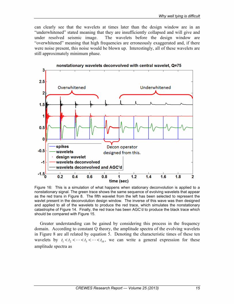
A better understanding of exactly why the nonstationary catastrophe occurs will help to appreciate its consequences and possible solutions. Towards this end, consider again the wavelet evolution shown in Figure 8. According to constant-Q theory the nonstationary seismogram contains a continuously evolving wavelet and Figure 8 shows a regularly spaced subset of those wavelets. Designing a deconvolution operator over a limited time zone, as was done to produce Figure 14, is very much like taking one of the central red wavelets in Figure 8, calculating its numerical inverse and applying this inverse to all of the wavelets. The result of doing exactly that is shown in Figure 16 as the red curve which directly simulates the nonstationary catastrophe. The black trace in Figure 16 is achieved by applying an AGC to the disastrous result of the red trace. We



can clearly see that the wavelets at times later than the design window are in an “underwhitened” stated meaning that they are insufficiently collapsed and will give and under resolved seismic image. The wavelets before the design window are “overwhitened” meaning that high frequencies are erroneously exaggerated and, if there were noise present, this noise would be blown up. Interestingly, all of these wavelets are still approximately minimum phase.

Figure 16: This is a simulation of what happens when stationary deconvolution is applied to a nonstationary signal. The green trace shows the same sequence of evolving wavelets that appear as the red trans in Figure 8. The fifth wavelet from the left has been selected to represent the wavlet present in the deconvolution design window. The inverse of this wave was then designed and applied to all of the wavelets to produce the red trace, which simulates the nonstationary catastrophe of Figure 14. Finally, the red trace has been AGC’d to produce the black trace which should be compared with Figure 15.

Greater understanding can be gained by considering this process in the frequency domain. According to constant Q theory, the amplitude spectra of the evolving wavelets in Figure 8 are all related by equation 5. Denoting the characteristic times of these ten wavelets by 1 2 5 10t t t t< < < < < , we can write a general expression for these

amplitude spectra as

Margrave


( ) ( ) [ ]/0ˆ ˆ, , 1, 2, 10kf t Q

kw f t w f e kπ−= ∈ , 10

where ( )0w f represents the initial spectrum of the source. Choosing wavelet 5 to

design our deconvolution operator, ( )D f . means that

( ) ( ) ( )5 /

5 0

1ˆ ˆ,

f t QeD fw f t w f

π+

= = 11

is the amplitude spectrum of the deconvolution operator. Thus the deconvolved wavelets have amplitude spectra given by

( ) ( ) ( ) ( ) [ ]5 /ˆ ˆ, , , 1, 2, 10kf t t QD k kw f t w f t D f e kπ− −= = ∈ . 12

So for 5kt t< , ( )ˆ ,D kw f t is a growing exponential while for 5kt t> we have exponential

decay. Only for 5kt t= do we achieve the desired flat spectrum. The phase associated

with the amplitude spectra in equation 12 should be locally minimum phase and hence nonstationary as well.

Figure 17 panel a) shows a direct numerical calculation of the evolving wavelets before deconvolution (i.e. the green trace in Figure 16) and panel b) shows the wavelets after deconvolution (the red trace of Figure 16). Equation 10 describes panel a) while equation 12 describes panel b).

Figure 17: A frequency domain explanation of the nonstationary catastrophe. In panel a) (left) are the amplitude spectra of the evolving wavelets in Figure 8. The red line indicates the spectrum of the wavelet chosen for the deconvolution operator. Deconvolution is then simulated by dividing each curve on the left by the red curve, and the result is in panel b) (right). Clearly all wavelets earlier than the design wavelet are exponentially overwhitened while the later wavelets are exponentially underwhitened. (“Exponentially” is used here because the vertical axis is a decibel log scale and the deconvolved spectra are straight lines on this figure.)



So, the nonstationary catastrophe is a consequence of trying to use a single representative of the evolving wavelet to deconvolve the wavelets at all times. The wavelet chosen for the deconvolution operator design is the source wavelet as modified by the anelastic attenuation along the travel path to the design window. When the resulting deconvolution operator is applied to earlier times, it removes too much attenuation and when applied to later times it does not do enough. The result is a very poor reflectivity estimate and a subsequent AGC is really just a cosmetic adjustment.

DEALING WITH THE NONSTATIONARY CATASTROPHE

I will discuss three approaches to dealing with this situation which are: (1) a simple time-variant balancing after deconvolution, (2) an inverse Q filter, (3) Gabor deconvolution. Of these, the first is not really a solution and is merely cosmetic, the second can work very well but requires knowledge of Q, and the third accomplishes a nonstationary deconvolution without knowing Q but can distort amplitudes.

Time variant balancing

Since the main visual effect of nonstationarity is a time-variant amplitude imbalance, we are lead to try an automatic gain correction whenever needed. The results are shown in Figure 18. Beginning with the raw trace at the top, the next trace shows the result of an AGC (0.3 second operator length) and this does indeed appear to have balanced the amplitudes. However, the stationary deconvolution still results in a nonstationary catastrophe although perhaps less severe. Another AGC afterwards serves as a cosmetic fix for the high amplitudes at the beginning of the trace but there is still an obvious frequency imbalance. The correlation coefficients, measured in the design window between each trace and the reflectivity, are quoted on the Figure. There is a general increase in correlation but the end values are quite small for a noise free simulation.

The final step in Figure 18 is an attempt to correct the residual phase errors by doing a time-variant phase adjustment based on comparing with the known reflectivity. This is analogous to comparing to well control. The phase measurements are shown in Figure 19. The method for phase measurement is very simple and is conducted repeatedly in a sliding Gaussian window. For each window position, the trace and the reflectivity are windowed and the windowed reflectivity is bandlimited to match the bandwidth of the windowed trace. Then these two signals are compared for all phase angles between -180 and 180 in 1 degree increments. The phase angle for which the L2 norm of the trace difference is minimal is chosen as the optimal angle for that window position. Having measured a time-variant phase, the trace phase is rotated in a time variant way and then the phase is re-measured as a quality check. Note that the residual phase measurement and correction actually causes a slight decrease in the correlation coefficient. This is likely an indication that the actual phase errors are more complex than can be accommodated by time-variant constant phase rotations.

For comparison in Figure 19, the measured time-variant phase for the stationary case (stationary seismogram and stationary deconvolution) are shown. The measured phase error in this case is very small and essentially stationary. After moving this phase, the re-measurement shows essentially zero. In the nonstationary case of Figure 18, the measured phase is nonstationary. Given that we might expect the phase to be more

Margrave


complex than a constant rotation and that the application of this phase actually decreases the correlation, the meaning of these phases could be challenged.

Figure 18: An attempt to deal with nonstationarity by using AGC for time-variant balancing before and after stationary deconvolution. The AGC before stationary deconvolution lessens the apparent severity of the nonstationary catastrophe but it is still apparent. The AGC afterward does a cosmetic adjustment of amplitudes. The cc values annotated are the maximum correlation coefficient measured in the design window when compared with the reflectivity.

Figure 19: The result of a time variant phase analysis to (top) the stationary seismogram after stationary deconvolution, and (bottom) the nonstationary trace after stationary deconvolution and amplitude balancing. In each case, constant phase rotations were estimated in a sliding Gaussian window by comparing to the actual reflectivity. The time-variant rotations were then applied and the result was re-measured. In the stationary case, the phase errors are essentially stationary while in the nonstationary case a time-variant phase error is measured.



Inverse Q filtering and Gabor Deconvolution

Inverse Q filtering is the common terminology for applying an operator meant to remove the Q effect, thereby rendering the trace stationary. Following the inverse Q filter, stationary deconvolution is then applied to estimate and remove the source wavelet. As discussed previously in the vicinity of equation 4, this approach implicitly assumes that the Q impulse response matrix,

QW , commutes with the convolution matrix for the

source wavelet, 0

W . In general, these matrices do not commute, however; as

demonstrated in Figure 6 they almost commute in at least this simple case. It is not known how this almost commutativity might change with a more complex Q structure, but there have been many successful tests of inverse Q filtering.

Another difficulty with this process is that the actual Q structure must be known. Measurement of Q is a difficult process and the reality is that the actual Q values can only be crudely estimated at present (e.g. Cheng and Margrave 2012, 2013). The implications of an erroneous Q value will not be examined here.

Despite these difficulties, it is worth examining the performance of inverse Q filtering in the context of the present discussion. The computation of efficient inverse Q filters is important for processing large datasets, but here the simple pseudo inverse of

QW will

illustrate the potential. Figure 20 shows the result of an inverse Q filter (actually matrix) applied to the nonstationary seismogram of Figure 11 and compares it to the stationary seismogram. As in the example of Figure 6 we see that the matrix commutation is almost exact.

Figure 20: The inverse Q matrix applied to the nonstationary trace of Figure 11 essentially

recovers the stationary trace due to the almost commuting nature of the matrices Q

W and 0

W .

The correlation coefficient between the inverse Q filters result and the stationary result is 0.99.

Margrave


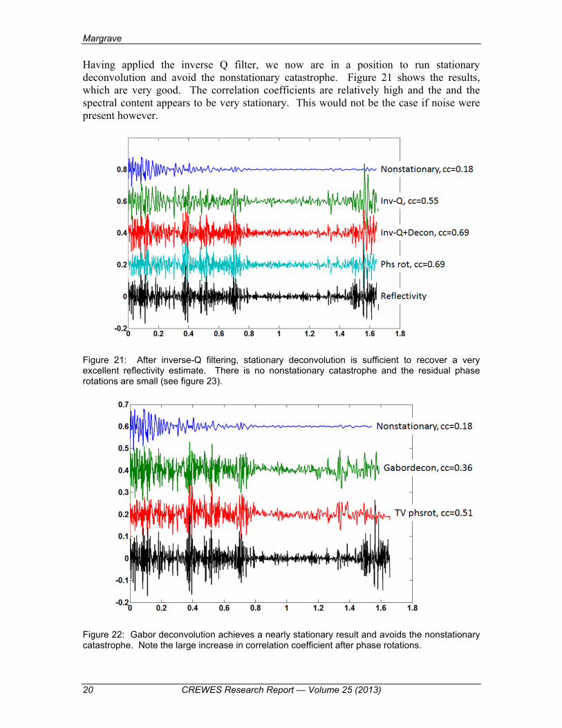
Having applied the inverse Q filter, we now are in a position to run stationary deconvolution and avoid the nonstationary catastrophe. Figure 21 shows the results, which are very good. The correlation coefficients are relatively high and the and the spectral content appears to be very stationary. This would not be the case if noise were present however.

Figure 21: After inverse-Q filtering, stationary deconvolution is sufficient to recover a very excellent reflectivity estimate. There is no nonstationary catastrophe and the residual phase rotations are small (see figure 23).

Figure 22: Gabor deconvolution achieves a nearly stationary result and avoids the nonstationary catastrophe. Note the large increase in correlation coefficient after phase rotations.



An alternative to inverse Q filtering is a nonstationary deconvolution like Gabor deconvolution (Margrave and Lamoureux, 2001; Margrave et al., 2011). This process attempts to combine the operations of Inverse Q filtering and stationary deconvolution into a single step. Unlike inverse Q filtering, Q information is not used because the algorithm uses a time-frequency decomposition of the data to measure the actual attenuation. Figure 22 shows the result of Gabor deconvolution applied to the nonstationary synthetic of Figure 11. While there is no nonstationary catastrophe and the spectral content of the trace appears visually stationary (compared with Figure 18) the correlation coefficient is only 0.36. However, after the time-variant constant-phase analysis and correction, the correlation increases substantially to 0.51. This is taken as an indication that the residual phase after Gabor decon is relatively simple and is correctable by this method. The reason for the residual phase is not presently known.

Figure 23: Time variant phase analysis after inverse Q filtering+stationary decon compared with the same analysis after Gabor decon. Gabor decon shows a much larger residual phase. However, it seems correctable upon comparison with well control.

NOISY SYNTHETICS

Incorporation of just a small amount of noise makes the inverse Q filter much less attractive. Figure 24 shows the same synthetic seismograms with a small amount of normally distributed random noise added in. The noise power was selected such that the time-domain signal-to-noise ratio in the design window of the nonstationary trace is 2.0. The same noise was added to the stationary trace so that it has a higher signal-to-noise ratio. Note that the visual appearance of either seismogram is changed very little.

In Figure 25 we see the performance of several different inverse Q filters. The filters differ by the choice of a tolerance parameter used in the Matlab function pinv that was used to calculate the inverse of the Q matrix. When designing the pseudo inverse of the Q matrix, pinv does not invert singular values less than the tolerance and instead sets them to zero. The tolerance value of 10 is the same value used in the results of Figure 21 that worked so well in the noise free case. This time the results are a mess because the operator has greatly amplified small amplitude noise. To get a stable result, a tolerance

Margrave


of 0.1 was used to get a stable result, but this has the effect of not rendering the trace stationary.

Figure 24: Identical Gaussian random noise has been added to both seismograms. The noise power is such that the signal-to-noise ratio is 2 in the design window of the nonstationary seismogram. This means that the stationary seismogram has a much higher signal-to-noise ratio.

Figure 25: The performance of 3 different inverse Q filters on the noisy nonstationary synthetic of Figure 24 is shown. The tolerance parameter is used in the design of the pseudo inverse of the Q matrix. A smaller tolerance is a more precise inverse. The tol=10 filter was the same as that



used for Figures 20 and 21, but this time it blows up the noise disastrously. A much larger tol is required for a stable result but this lessens the performance of the inverse Q filter.

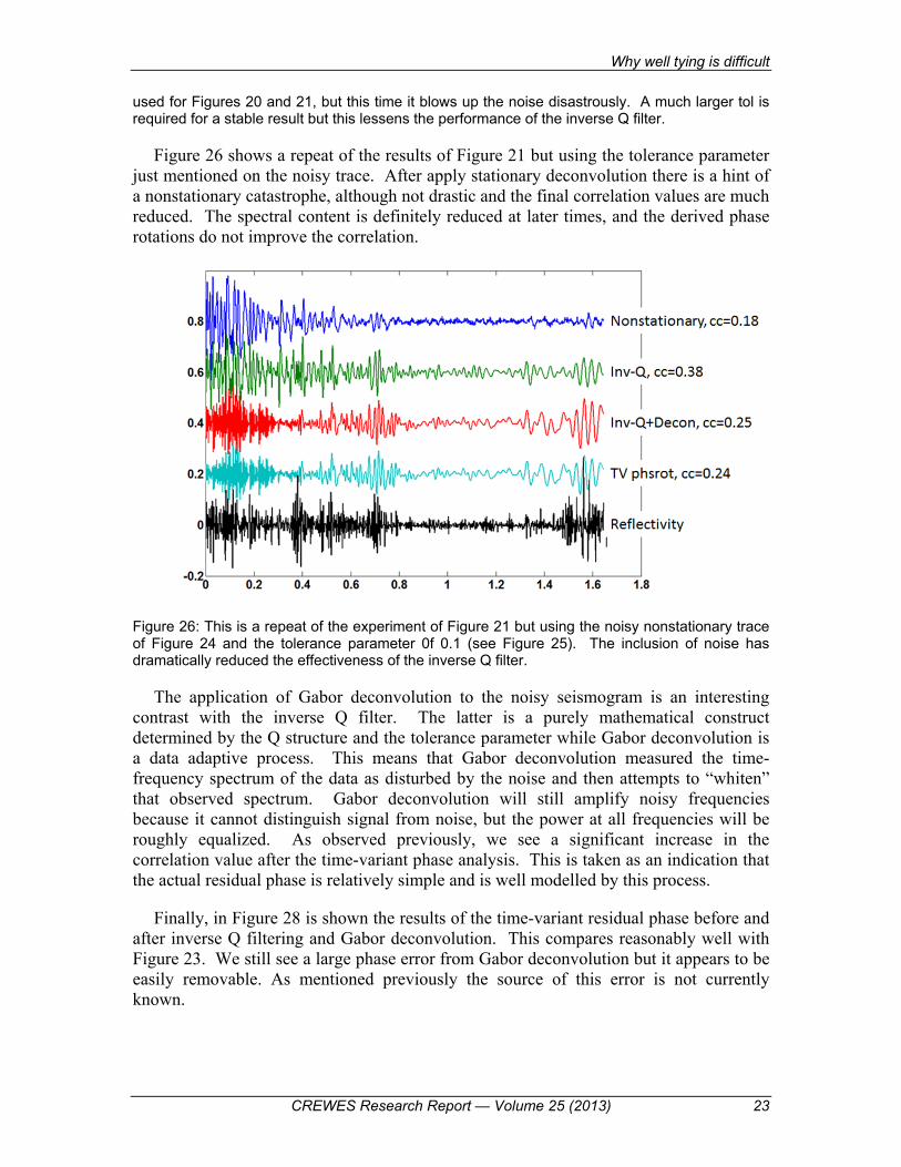
Figure 26 shows a repeat of the results of Figure 21 but using the tolerance parameter just mentioned on the noisy trace. After apply stationary deconvolution there is a hint of a nonstationary catastrophe, although not drastic and the final correlation values are much reduced. The spectral content is definitely reduced at later times, and the derived phase rotations do not improve the correlation.

Figure 26: This is a repeat of the experiment of Figure 21 but using the noisy nonstationary trace of Figure 24 and the tolerance parameter 0f 0.1 (see Figure 25). The inclusion of noise has dramatically reduced the effectiveness of the inverse Q filter.

The application of Gabor deconvolution to the noisy seismogram is an interesting contrast with the inverse Q filter. The latter is a purely mathematical construct determined by the Q structure and the tolerance parameter while Gabor deconvolution is a data adaptive process. This means that Gabor deconvolution measured the time-frequency spectrum of the data as disturbed by the noise and then attempts to “whiten” that observed spectrum. Gabor deconvolution will still amplify noisy frequencies because it cannot distinguish signal from noise, but the power at all frequencies will be roughly equalized. As observed previously, we see a significant increase in the correlation value after the time-variant phase analysis. This is taken as an indication that the actual residual phase is relatively simple and is well modelled by this process.

Finally, in Figure 28 is shown the results of the time-variant residual phase before and after inverse Q filtering and Gabor deconvolution. This compares reasonably well with Figure 23. We still see a large phase error from Gabor deconvolution but it appears to be easily removable. As mentioned previously the source of this error is not currently known.

Margrave


Figure 27: This shows the results of Gabor deconvolution on the noisy nonstationary synthetic and should be compared with Figures 22 and 26. The presence of noise degrades the performance of Gabor deconvolution but not as drastically as it does for the inverse Q filter. This is because Gabor deconvolution adapts to the data while the inverse Q filter does not.

Figure 28: Time-variant residual phase analysis is shown before and after the application of the inverse Q filter and Gabor deconvolution to the noisy nonstationary seismogram. Compare with the noise free case of Figure 23

CONCLUSIONS

It has been argued that anelastic attenuation is the cause of well-tying difficulties such as spectral balancing and phase matching. Using stationary deconvolution on a nonstationary trace leads to large nonstationary amplitude and phase errors that are difficult to correct, even with well control. Termed the nonstationary catastrophe, it was



shown that these errors are directly attributable to deconvolving a temporally evolving wavelet with an inverse operator designed from a snapshot of the wavelet in a target zone. This causes an exponential (with time and frequency) increase in amplitude at times before the design time and an exponential decrease at later times. These nonstationary amplitude errors are paired with nonstationary minimum phase spectra. The common practice of an AGC after the deconvolution does balance the amplitudes in time but leaves the amplitude spectrum nonstationary and does not address the phase errors. Attempts to correct the phase errors by nonstationary constant phase rotations were generally unsuccessful.

The theoretically better approach is to apply an inverse Q filter followed by stationary deconvolution. This avoids the nonstationary catastrophe and gives a reflectivity estimate with small amplitude and phase errors. However it requires knowledge of Q. Gabor deconvolution provides an alternative that also avoids the nonstationary catastrophe, does not require knowledge of Q, but has larger amplitude and phase errors than inverse Q filtering. However, the residual phase after Gabor deconvolution appears to be correctible by nonstationary constant phase analysis in comparison with well control.

The inclusion of noise leads to greater problems for inverse Q filtering than for Gabor deconvolution. Fundamentally, this is because Gabor deconvolution adapts to the data while an inverse Q filter does not. Application of an inverse Q filter with even a small amount of noise leads to unstable amplification of the noise. Gabor deconvolution measures the inherent attenuation of the data in time and frequency and designs a data dependent operator to remove it. There are other similar processes that are also data dependent in the same class as Gabor deconvolution.

It has been argued here that better well ties will come from data processing that recognizes and addresses the fundamental nonstationarity of seismic data. Such processes will need to be data adaptive to cope with noise.

ACKNOWLEDGEMENTS

I am grateful to the Sponsors of CREWES and NSERC for their continued support. I also thank those who have worked with me over the years in the analysis of nonstationary effects including: Michael Lamoureux, Jeff Grossman, Victor Iliescu, Rob Ferguson, Alana Schoepp, Carlos Montana, Linping Dong, Safa Ismail, Peter Gibson, Chad Hogan, Heather Lloyd, Peng Cheng, Todor Todorov, and Hugh Geiger.

REFERENCES

Aki K. and P. G. Richards, 2002, Quantitative Seismology 2nd Edition, University Science Books. Cheng, P., and G. F. Margrave, 2012, Estimation of Q: a comparison of different computational methods:

in the 24th Annual Research Report of the CREWES Project. Cheng, P., and G. F. Margrave, 2013, Comparison of Q-estimation methods: an update: in the 25th Annual

Research Report of the CREWES Project. Futterman, W. I., 1962, Dispersive body waves: J. Geophys. Res., 67, 5279-91. Esmaeli, S., and G. F. Margrave, 2013, Recovering low frequency for impedance inversion by frequency

domain deconvolution, in the 25th Annual Report of the CREWES Project. Kjartansson, E, 1979, Constant Q-wave Propagation and Attenuation, Journal of Geophysical Research, 84,

4737-4748.

Margrave


Lloyd, H, J, E, 2013, An investigation of the role of low frequencies in seismic impedance inversion, MSc thesis, University of Calgary, available at www.crewes.org.

Lloyd, H. J. E., and G. F. Margrave, 2012a, Incorporating spectral colour into impedance inversion: Hussar Example: in the 24th Annual Research Report of the CREWES Project.

Lloyd, H. J. E., and G. F. Margrave, 2012b, Investigating the low frequency content of the Hussar data with impedance inversion: in the 24th Annual Research Report of the CREWES Project.

Margrave, G. F. and Lamoureux, M. P., 2001, Gabor Deconvolution: in the 13th Annual Research Report of the CREWES Project.

Margrave, G. F., Lamoureux, M. P., and Henley, D. C., 2011, Gabor deconvolution: Estimating reflectivity by nonstationary deconvolution of seismic data: Geophysics, 76, 15-30.

Margrave, G. F., 2013, Q tools: Summary of CREWES software for Q modelling and analysis, in the 25th Annual Report of the CREWES Project.

O’Doherty, R. F., and N. A. Anstey, 1971, Reflections on amplitudes, Geophysical Prospecting, 19, 430-458.

White, R. E., R. Simm, and S. Xu, 1998, Well tie, fluid substitution and AVO modelling: a North Sea example: Geophysical Prospecting 46, 323-436.

White, R. E., 1980, Partial coherence matching of synthetic seismograms with seismic traces, Geophysical Prospecting, 28, 333-358.

Date post:	21-Mar-2020
Category:	Documents
Upload:	others
View:	15 times
Download:	5 times

Why seismic-to-well ties are difficult - CREWES · Why seismic-to-well ties are difficult Gary F....

Documents