Why Your Wifi Sucks and How It Can Be Helped, Part 1 (Tom’s Hardware article July 2011) Please Power Down ‐ “All you bloggers need to turn off your base stations,” an increasingly annoyed Steve Jobs told the crowd at the June 2010 iPhone 4 demo. “If you want to see the demos, shut off your laptops, turn off all these MiFi base stations, and put them on the floor, please.” In a crowd of 5000 people, roughly 500 Wi‐Fi devices were active. It was the wireless apocalypse, and not even a fleet of Silicon Valley’s finest backstage engineers could do a thing about it. If this example of 802.11 extremity sounds inapplicable to your everyday world, refer back to August 2009, when Tom’s Hardware took its first look at Ruckus Wireless's beamforming technology in Beamforming: The Best WiFi You’ve Never Seen. In that story, we introduced the concepts of beamforming and examined some competitive test results in a big office environment. As enlightening as this was at the time, there is clearly much more of the tale to be told. This literally came home to me a few months ago after setting up a nettop for my children and using a dual‐spectrum (2.4 GHz and 5.0 GHz) Linksys 802.11n USB dongle to connect to my Cisco small business‐class 802.11n access point. The wireless performance was horrific. We couldn’t even stream YouTube videos. I assumed the problem was the nettop’s feeble processing and graphics capabilities. One day, I tried substituting the 7811 wireless bridge kit from that previous piece. The difference was instantaneous, and video looked perfectly fluid. It was as if I had plugged in a wired Ethernet connection. What was going on here? I wasn’t in an auditorium filled with 500 live bloggers crushing my connection. I was using supposedly best‐of‐breed small business Cisco/Linksys gear that I’d personally tested and knew had higher performance than most competing brands. It wasn’t enough to have switched to the Ruckus‐based wireless bridge. That left too many unanswered questions. Why was one product performing better than the other? Why had editor Chris Angelini himself observed in our original article that not only did the up‐close proximity between his client and the access point impact performance but so did the shape of the AP itself? Unanswered Questions ‐ Six months ago, Ruckus tried to set up a test scenario to help us answer those unanswered questions through analysis of RF interference on Wi‐Fi performance, but just before the tests were set to begin, the company halted its experiment. Engineers had set up RF noise generators and sample client machines, but a test result measurement taken one minute would come back two minutes later with numbers that were wildly different. Even averaging a set of five results in a given location would be meaningless. This is why you never see real‐
Transcript
Why Your Wifi Sucks and How It Can Be Helped, Part 1 (Tom’s Hardware article July 2011)
Please Power Down ‐ “All you bloggers need to
turn off your base stations,” an increasingly
annoyed Steve Jobs told the crowd at the June
2010 iPhone 4 demo. “If you want to see the
demos, shut off your laptops, turn off all these
MiFi base stations, and put them on the floor,
please.”
In a crowd of 5000 people, roughly 500 Wi‐Fi
devices were active. It was the wireless
apocalypse, and not even a fleet of Silicon
Valley’s finest backstage engineers could do a
thing about it.
If this example of 802.11 extremity sounds
inapplicable to your everyday world, refer back to
August 2009, when Tom’s Hardware took its first
look at Ruckus Wireless's beamforming technology in Beamforming: The Best WiFi You’ve Never Seen. In that story, we
introduced the concepts of beamforming and examined some competitive test results in a big office environment. As
enlightening as this was at the time, there is clearly much more of the tale to be told.
This literally came home to me a few months ago after setting up a nettop for my children and using a dual‐spectrum
(2.4 GHz and 5.0 GHz) Linksys 802.11n USB dongle to connect to my Cisco small business‐class 802.11n access point. The
wireless performance was horrific. We couldn’t even stream YouTube videos. I assumed the problem was the nettop’s
feeble processing and graphics capabilities. One day, I tried substituting the 7811 wireless bridge kit from that previous
piece. The difference was instantaneous, and video looked perfectly fluid. It was as if I had plugged in a wired Ethernet
connection.
What was going on here? I wasn’t in an auditorium filled with 500 live bloggers crushing my connection. I was using
supposedly best‐of‐breed small business Cisco/Linksys gear that I’d personally tested and knew had higher performance
than most competing brands. It wasn’t enough to have switched to the Ruckus‐based wireless bridge. That left too many
unanswered questions. Why was one product performing better than the other? Why had editor Chris Angelini himself
observed in our original article that not only did the up‐close proximity between his client and the access point impact
performance but so did the shape of the AP itself?
Unanswered Questions ‐ Six months ago, Ruckus tried to
set up a test scenario to help us answer those
unanswered questions through analysis of RF
interference on Wi‐Fi performance, but just before the
tests were set to begin, the company halted its
experiment. Engineers had set up RF noise generators
and sample client machines, but a test result
measurement taken one minute would come back two
minutes later with numbers that were wildly different.
Even averaging a set of five results in a given location
would be meaningless. This is why you never see real‐
world interference studies done in the press. It’s so hard to control the environment and the variables that testing is
effectively impossible. Vendors can spout all of the performance numbers they like from optimally‐configured testing
done in RF isolation chambers, but those statistics are meaningless out in the real world.
Frankly, we've never seen these issues explained and explored before, so we chose to pick up the reins, shed some light
on Wi‐Fi performance, and expose its inner mysteries. This is not going to be a short trip. We have a lot of ground to
cover, which is why we’re going to break the story into two pieces. Today, we’ll be exploring the theoretical aspects
(how Wi‐Fi works at the data and hardware levels). Then we’ll proceed to put this theory to the test in the most extreme
wireless environment we’ve ever encountered, which includes 60 notebooks and nine tablets all pounding a single
access point. Whose technology will stand up and whose will crumble and cry for mercy? By the time we’re done, you’ll
not only have the answer, but you’ll understand why we saw those results and how the technologies behind those
results work. Hang on tight. It’s going to get a bit congested in here.
Congestion Vs. Contention ‐ We normally use
the word “congestion” when describing
wireless traffic overload situations, but, when
you get down into the networking nitty‐gritty,
congestion doesn’t really mean anything. The
better term is “contention.” Packets must
contend with each other for permission to
send and receive during open opportunities,
like gaps in traffic. Remember that Wi‐Fi is a
half‐duplex technology, so at any given
moment, only one device on a channel can
transmit, either the AP or one of its clients.
The more devices on a wireless LAN, the more
important contention management becomes,
as many clients compete for airtime.
Given the ever‐increasing proliferation of Wi‐Fi networks, exactly who gets to transmit, and when, is hugely important.
There is only one rule: whoever talks into silence wins. If no one else is trying to transmit when you do, then you get to
talk unhindered. But if two or more clients try to talk at the same time, you have a problem. It’s like talking to your
buddy with a walkie‐talkie. When you talk, your friend has to wait and listen. If you both try to talk at the same time,
neither one of you will be heard. To communicate with each other effectively, the two of you must manage your airtime
access and contention. This is why you say something like “over” when you’re done talking. You signal that the air is free
for someone else to talk.
If you’ve ever taken walkie‐talkies on a trip, you may have noticed there were only a few available channels—and lots of
other people who had the same idea. Especially in the days before cheap cell phones, it felt like everybody was on
walkie‐talkies. You and your friend might not talk over each other, but that still left every other walkie‐talkie user near
you who happened to be using the same channel. Every time you wanted to get a word in, someone would already be
on your channel, forcing you to wait...and wait...and wait.
This kind of interference is called “co‐channel” interference, wherein interferers clog your channel. To get around the
problem, you can try moving to another channel, but if nothing better is available, you're stuck with very, very slow
communication speeds. You only get to transmit when all of those longwinded so‐and‐sos around you all have a rare
moment of silence. You might only want to say one small thing, like “Holy cow, co‐channel interference bites!” But you
might have to wait 15 minutes for an opening in which make your quick, pithy statement.
Interference Sources ‐ Compounding the co‐
channel problem is the fact that Wi‐Fi traffic
flow is never smooth. We have radio frequency
(RF) interference randomly interjecting itself into
packet paths, striking anywhere at any time for
any duration. Interference can come from a wide
variety of sources, everything from cosmic rays
to competing Wi‐Fi networks. For example,
microwave ovens and cordless phones are
notorious offenders for the 2.4 GHz Wi‐Fi
spectrum.
To illustrate, imagine you’re playing Hot Wheels
cars with a friend, and each car that you shove
across the floor to your friend represents a
packet. Interference is like your little brother
playing marbles with his friend across your line
of traffic. A marble might not hit your Hot
Wheels rig at any given time, but eventually you
will get nailed. When a collision does happen, you have to stop what you’re doing, take the car that got hit back to the
starting line, and try sending it again. And just to be a brat, your little brother doesn’t always use marbles. Sometimes he
sends in a beach ball or a dog.
Effective wireless networking is all about managing the Wi‐Fi or RF spectrum—getting the user on and off the wireless
road as quickly as possible. How do you get your Hot Wheels to travel faster and aim more accurately? How do you get
more cars passed back and forth and ignore your little brother’s feeble efforts to interfere with your day? Therein lies
the secret sauce of wireless networking vendors.
The Difference Between Wi‐Fi Traffic And
Interference ‐ We’ll come back to this in a bit,
but understand up front that the 802.11
standard does many things to regulate how
packets get handled. Again, take an automotive
metaphor. When you drive a car onto the road,
you have lanes, speed laws, and other rules that
govern how your car should behave within
certain parameters. But if your great
grandmother with her Coke bottle glasses and
Lawrence Welk eight‐track plods down the
interstate doing 35 in a 65, the other drivers will
get upset and honk. Traffic slows down. But
everyone keeps driving, even if at a reduced
speed.
This is analogous to what happens when your neighbor’s Wi‐Fi traffic enters your own wireless LAN. Because all of the
traffic is 802.11, all packets are governed by the same rules. That unwanted traffic gets in your way and slows down
overall packet flow, but it doesn’t have the same impact as microwave oven emissions, which play by no rules and
simply plow across the various Wi‐Fi traffic lanes (channels) like a line of suicidal pedestrians.
Obviously, the relative impact of RF noise in Wi‐Fi’s 2.4 or 5.0 GHz ranges is worse than that of competing WLAN traffic,
but one of the objects in improving performance is mitigating both. As we’ll see, there are many ways to do this. For
now, just keep in mind that all of this competing traffic and interference ultimately becomes background noise. A packet
stream that starts out strong at ‐30 dB will ultimately fade to ‐100 dB and less over distance. Such levels are far too low
to be intelligible to an access point, but it can still disrupt traffic, just like that old lady in the Coke bottle glasses.
All’s Fair In War And Airtime ‐ Let’s talk about how access points
(including the access points buried in routers) administer traffic
rules. Consider your typical two‐lane freeway onramp. You have
cars lined up in each lane, and each lane has a stop/go light timed
to regulate how traffic enters the main roadway. Each green light
lasts for, say, five seconds.
Wi‐Fi tweaks this idea slightly with a process called airtime
fairness. The access point assesses the number of client devices
present and assigns equal time blocks for each device, as if a
camera overlooking the onramp could judge the amount of
backed up traffic and use that information to decide how long
each green light should last. As long as the light is green, cars can
keep moving from that onramp into traffic. When the light turns
red, that onramp lane stops and the next lane turns green.
Now say we have three lanes in that onramp, one each for
802.11b, 11g, and 11n. Obviously, the packets travel at different
speeds, like one lane being for zippy sports cars and another for
slow 18‐wheelers. You’re going to get more fast packets than slow
packets into traffic during a given time period.
Without airtime fairness, traffic sinks to the lowest common denominator. All vehicles line up in one lane, and if a fast
car (11n) gets stuck behind a semi (11b), the whole chain slows down to the semi’s speed. This is why, if you’ve done
much traffic analysis with consumer routers and APs, you find that performance can tank when you bring an old 11b
device onto an 11n network, which is why many APs feature an “11n only” mode. Doing this, of course, forces the AP to
ignore the slower device. Unfortunately, most consumer Wi‐Fi products do not yet support airtime fairness. This is an
increasingly common feature in the enterprise world that will hopefully trickle down to the masses soon.
When Bad Things Happen To Good Packets ‐ Enough about cars. Let’s
look at packets and interference in a slightly different way. As said before,
interference can strike at any time and last for any amount of time. You
see this in the following page’s image with its blue bars, which represent
interference. When interference strikes a data packet, the packet
becomes corrupted and must be resent, causing latencies and increasing
total send time.
When we say we want faster wireless performance, that largely means we
want our packets to get from the AP to the client (or vice versa) more
quickly. To make this possible, APs tend to use any or all of three tactics:
lowering the PHY data rate, lowering transmit power (Tx), and changing
the radio channel.
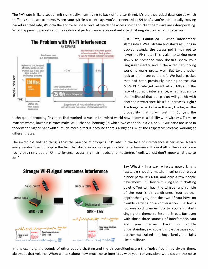
The PHY rate is like a speed limit sign (really, I am trying to back off the car thing). It’s the theoretical data rate at which
traffic is supposed to move. When your wireless client says you’ve connected at 54 Mb/s, you’re not actually moving
packets at that rate; it’s only the approved speed level at which the access point and client hardware are interoperating.
What happens to packets and the real‐world performance rates realized after that negotiation remains to be seen.
PHY Rate, Continued ‐ When interference
slams into a Wi‐Fi stream and starts resulting in
packet resends, the access point may opt to
lower the PHY rate. This is akin to talking more
slowly to someone who doesn’t speak your
language fluently, and in the wired networking
world, it works pretty well. But take another
look at the image to the left. We had a packet
that had been previously running at the 150
Mb/s PHY rate get resent at 25 Mb/s. In the
face of sporadic interference, what happens to
the likelihood that our packet will get hit with
another interference blast? It increases, right?
The longer a packet is in the air, the higher the
probability that it will get hit. So yes, the
technique of dropping PHY rates that worked so well in the wired world now becomes a liability with wireless. To make
matters worse, lower PHY rates make Wi‐Fi channel bonding (in which two channels in a 2.4 or 5.0 GHz band are used in
tandem for higher bandwidth) much more difficult because there’s a higher risk of the respective streams working at
different rates.
The incredible and sad thing is that the practice of dropping PHY rates in the face of interference is pervasive. Nearly
every vendor does it, despite the fact that doing so is counterproductive to performance. It’s as if all of the vendors are
facing this rising tide of RF interference, scratching their heads, and muttering, “well, we just don’t know what else to
do!”
Say What? ‐ In a way, wireless networking is
just a big shouting match. Imagine you’re at a
dinner party. It’s 6:00, and only a few people
have shown up. They’re mulling about, chatting
quietly. You can hear the whisper and rumble
of the room’s air conditioner. Your partner
approaches you, and the two of you have no
trouble carrying on a conversation. The host’s
four‐year‐old wanders up to you and starts
singing the theme to Sesame Street. But even
with those three sources of interference, you
and your partner have no trouble
understanding each other, in part because your
partner was raised in a huge family and talks
like a bullhorn.
In this example, the sounds of other people chatting and the air conditioning are the “noise floor.” It’s always there,
always at that volume. When we talk about how much noise interferes with your conversation, we discount the noise
floor. It’s like putting the tray on a food scale and then hitting the button to zero the weight readout. The scale's tray
and background noise are constants, just like the background RF noise present all around us. Every environment has its
own noise floor.
However, the kid and his Big Bird homage are interference. With a partner speaking loudly, you can still converse
effectively, but what happens when a soft‐spoken friend walks up and joins the discussion? You find yourself casting
annoyed glances at the (previously charming) toddler and asking “what?” to your new conversation mate.
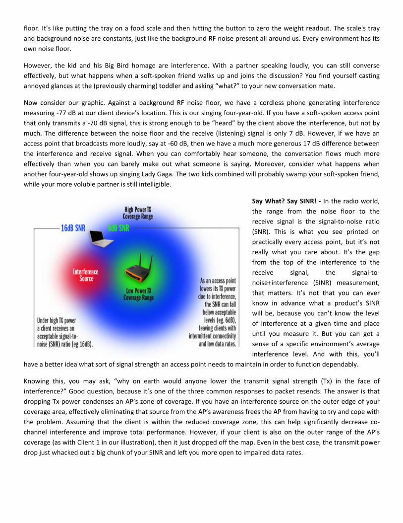
Now consider our graphic. Against a background RF noise floor, we have a cordless phone generating interference
measuring ‐77 dB at our client device’s location. This is our singing four‐year‐old. If you have a soft‐spoken access point
that only transmits a ‐70 dB signal, this is strong enough to be “heard” by the client above the interference, but not by
much. The difference between the noise floor and the receive (listening) signal is only 7 dB. However, if we have an
access point that broadcasts more loudly, say at ‐60 dB, then we have a much more generous 17 dB difference between
the interference and receive signal. When you can comfortably hear someone, the conversation flows much more
effectively than when you can barely make out what someone is saying. Moreover, consider what happens when
another four‐year‐old shows up singing Lady Gaga. The two kids combined will probably swamp your soft‐spoken friend,
while your more voluble partner is still intelligible.
Say What? Say SINR! ‐ In the radio world,
the range from the noise floor to the
receive signal is the signal‐to‐noise ratio
(SNR). This is what you see printed on
practically every access point, but it’s not
really what you care about. It’s the gap
from the top of the interference to the
receive signal, the signal‐to‐
noise+interference (SINR) measurement,
that matters. It’s not that you can ever
know in advance what a product’s SINR
will be, because you can’t know the level
of interference at a given time and place
until you measure it. But you can get a
sense of a specific environment’s average
interference level. And with this, you’ll
have a better idea what sort of signal strength an access point needs to maintain in order to function dependably.
Knowing this, you may ask, “why on earth would anyone lower the transmit signal strength (Tx) in the face of
interference?” Good question, because it’s one of the three common responses to packet resends. The answer is that
dropping Tx power condenses an AP’s zone of coverage. If you have an interference source on the outer edge of your
coverage area, effectively eliminating that source from the AP’s awareness frees the AP from having to try and cope with
the problem. Assuming that the client is within the reduced coverage zone, this can help significantly decrease co‐
channel interference and improve total performance. However, if your client is also on the outer range of the AP’s
coverage (as with Client 1 in our illustration), then it just dropped off the map. Even in the best case, the transmit power
drop just whacked out a big chunk of your SINR and left you more open to impaired data rates.
So Many Channels, So Little To Watch ‐ As we’ve
seen, the first two common approaches for
dealing with interference are lowering the PHY
rate and lowering power. The third approach is
one we touched on in the walkie‐talkie example:
change the wireless channel, which in effect
changes the frequency on which the signal is
being carried. This is the key idea behind spread
spectrum technology, or frequency hopping,
which was invented by Nikola Tesla at the turn of
the 20th century and gained notable military use
during World War II. In one instance, famous and
beautiful actress Hedy Lamarr helped invent a
frequency hopping approach to thwart enemy
jamming of radio‐controlled torpedoes. When
frequency hopping is employed over a wider
range of frequencies than that on which the signal is normally carried, this is known as spread spectrum.
Wi‐Fi uses spread spectrum technology primarily to improve bandwidth, reliability, and security. As anyone who’s ever
been under the hood of his or her Wi‐Fi settings knows, the 2.4 to 2.4835 GHz band has 11 channels. However, because
the total bandwidth used for 2.4 GHz Wi‐Fi spread spectrum is 22 MHz, you get overlapping between these channels. In
reality, you only have three channels in North America—1, 6, and 11—which will not overlap. Europe can use channels
1, 5, 9, and 13. If you’re using 2.4 GHz 802.11n with a “bonded” 40 MHz channel width, your options shrink to only two:
channels 3 and 11.
In the 5 GHz range, things improve somewhat. Here, we have eight non‐overlapping indoor channels (36, 40, 44, 48, 52,
56, 60, and 64.) Higher‐end access points usually integrate both 2.4 GHz and 5.0 GHz radios, and the correct assumption
is that there is less interference on the 5.0 GHz band. Just getting rid of 2.4 GHz Bluetooth interference can make a
difference. Unfortunately, the end result is inevitable: the 5.0 GHz spectrum is now filling up with traffic, just as the 2.4
GHz spectrum did. With 40 MHz channel bonding used in 802.11n, the number of non‐overlapping channels shrinks to
just four (dynamic frequency selection, or DFS, channels are excluded due to military worries about conflicting with
radar signals), and users are already finding times when there isn’t a decently open channel within range. It’s like having
more channels of TV to watch all day but still nothing on except personal hygiene commercials. Nobody wants to see
that.
Omnidirectional, Not Omnipotent ‐ We’ve covered a fair
amount of bad news so far. There’s more. It’s time to discuss
antennas.
We mentioned signal strength, but not signal direction. As
you probably know, most antennas are omnidirectional. Like
a ring of speakers blaring in every direction at once (with
attached microphones receiving from all 360 degrees
equally), omnidirectional microphones give you excellent
coverage. It doesn’t matter where the client is located. As
long as the client is within range, an omnidirectional antenna
should be able to find and communicate with it. The
downside, of course, is that the same omnidirectional
antenna is also picking up every other source of noise and interference within range. Omnidirectional systems hear
everything—good, bad, and ugly—and there’s very little you can do about it.
Imagine standing in a crowd, and you’re trying to talk with someone several feet away. You can barely hear someone
over the ambient noise. What’s the natural thing to do? Cup a hand to your ear, of course. You’re trying to better focus
the sound coming from one direction, while simultaneously blocking sounds coming from other directions, namely
behind your hand. An even better sound isolator is a stethoscope. These try to block all ambient sound by plugging your
ears, only allowing passing sounds carried through the flat chestpiece. In the world of radio, the equivalent of a
stethoscope is a technique called beamforming.
Beamforming Revisited ‐ We covered beamforming in considerable
depth during our prior visit with Ruckus, so we’ll only briefly review
here.
The object in beamforming is to create a directed zone of
heightened wave energy. The classic example of this is shown with
water drops into a pool. If you were to hold two spigots over a pool
of water and opened each spigot in just the right way that they
released synchronized water droplets every so often, the concentric
wave rings that flowed from each epicenter (where the droplets
land) would create an overlapping pattern. You can see this pattern
in the above illustration. Where the wave crests overlap, you have
an additive effect, where the energy of both waves combine to
create an even larger crest in the waveform. Because of the
regularity of the drops, these amplified crests manifest in certain
directions, forming a sort of “beam” of heightened energy.
The waves in this example are omnidirectional. They flow outward uniformly from the point of origin until reaching
some opposing object or energy. Wi‐Fi signals emitted from an omnidirectional antenna behave in the same way,
outputting waves of radio energy that, when combined with waves from another antenna source, can create beams of
heightened signal strength. When you have two waveforms in phase, the result can be a beam with nearly double the
signal strength of the original wave.
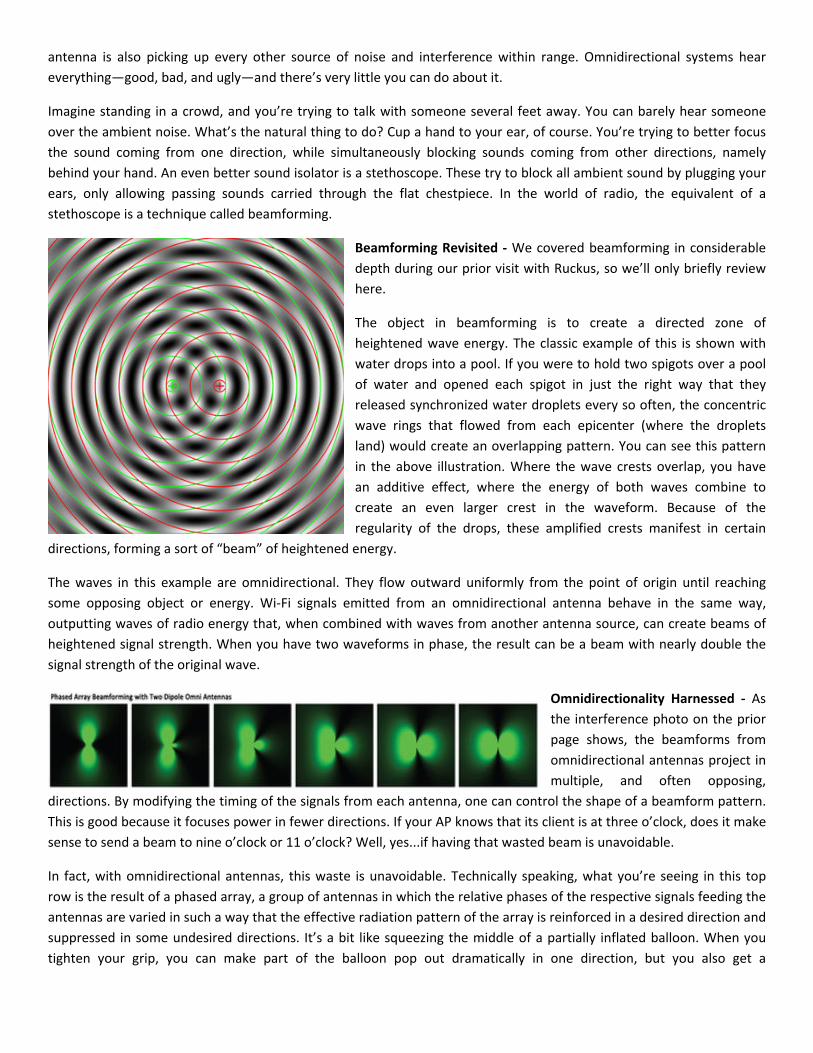
Omnidirectionality Harnessed ‐ As
the interference photo on the prior
page shows, the beamforms from
omnidirectional antennas project in
multiple, and often opposing,
directions. By modifying the timing of the signals from each antenna, one can control the shape of a beamform pattern.
This is good because it focuses power in fewer directions. If your AP knows that its client is at three o’clock, does it make
sense to send a beam to nine o’clock or 11 o’clock? Well, yes...if having that wasted beam is unavoidable.
In fact, with omnidirectional antennas, this waste is unavoidable. Technically speaking, what you’re seeing in this top
row is the result of a phased array, a group of antennas in which the relative phases of the respective signals feeding the
antennas are varied in such a way that the effective radiation pattern of the array is reinforced in a desired direction and
suppressed in some undesired directions. It’s a bit like squeezing the middle of a partially inflated balloon. When you
tighten your grip, you can make part of the balloon pop out dramatically in one direction, but you also get a
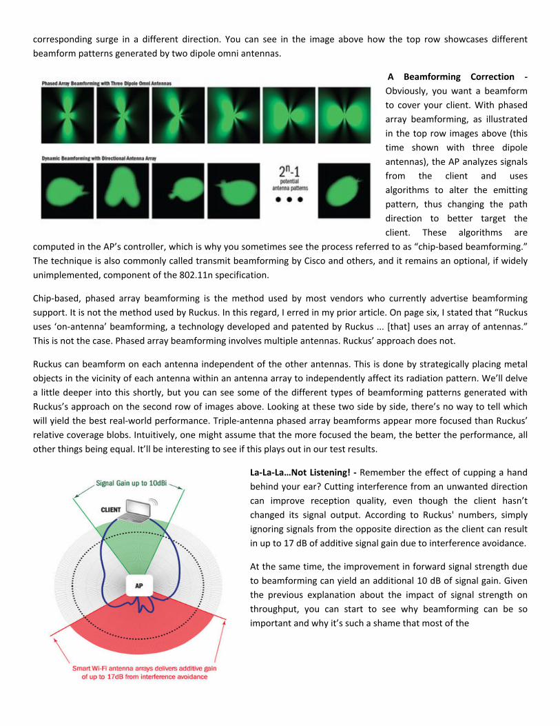
corresponding surge in a different direction. You can see in the image above how the top row showcases different
beamform patterns generated by two dipole omni antennas.
A Beamforming Correction ‐
Obviously, you want a beamform
to cover your client. With phased
array beamforming, as illustrated
in the top row images above (this
time shown with three dipole
antennas), the AP analyzes signals
from the client and uses
algorithms to alter the emitting
pattern, thus changing the path
direction to better target the
client. These algorithms are
computed in the AP’s controller, which is why you sometimes see the process referred to as “chip‐based beamforming.”
The technique is also commonly called transmit beamforming by Cisco and others, and it remains an optional, if widely
unimplemented, component of the 802.11n specification.
Chip‐based, phased array beamforming is the method used by most vendors who currently advertise beamforming
support. It is not the method used by Ruckus. In this regard, I erred in my prior article. On page six, I stated that “Ruckus
uses ‘on‐antenna’ beamforming, a technology developed and patented by Ruckus ... [that] uses an array of antennas.”
This is not the case. Phased array beamforming involves multiple antennas. Ruckus’ approach does not.
Ruckus can beamform on each antenna independent of the other antennas. This is done by strategically placing metal
objects in the vicinity of each antenna within an antenna array to independently affect its radiation pattern. We’ll delve
a little deeper into this shortly, but you can see some of the different types of beamforming patterns generated with
Ruckus’s approach on the second row of images above. Looking at these two side by side, there’s no way to tell which
will yield the best real‐world performance. Triple‐antenna phased array beamforms appear more focused than Ruckus’
relative coverage blobs. Intuitively, one might assume that the more focused the beam, the better the performance, all
other things being equal. It’ll be interesting to see if this plays out in our test results.
La‐La‐La…Not Listening! ‐ Remember the effect of cupping a hand
behind your ear? Cutting interference from an unwanted direction
can improve reception quality, even though the client hasn’t
changed its signal output. According to Ruckus' numbers, simply
ignoring signals from the opposite direction as the client can result
in up to 17 dB of additive signal gain due to interference avoidance.
At the same time, the improvement in forward signal strength due
to beamforming can yield an additional 10 dB of signal gain. Given
the previous explanation about the impact of signal strength on
throughput, you can start to see why beamforming can be so
important and why it’s such a shame that most of the
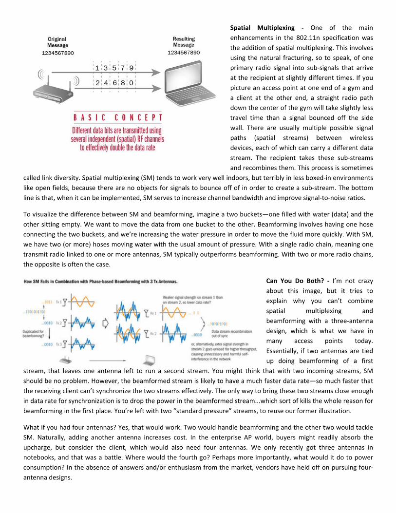
Spatial Multiplexing ‐ One of the main
enhancements in the 802.11n specification was
the addition of spatial multiplexing. This involves
using the natural fracturing, so to speak, of one
primary radio signal into sub‐signals that arrive
at the recipient at slightly different times. If you
picture an access point at one end of a gym and
a client at the other end, a straight radio path
down the center of the gym will take slightly less
travel time than a signal bounced off the side
wall. There are usually multiple possible signal
paths (spatial streams) between wireless
devices, each of which can carry a different data
stream. The recipient takes these sub‐streams
and recombines them. This process is sometimes
called link diversity. Spatial multiplexing (SM) tends to work very well indoors, but terribly in less boxed‐in environments
like open fields, because there are no objects for signals to bounce off of in order to create a sub‐stream. The bottom
line is that, when it can be implemented, SM serves to increase channel bandwidth and improve signal‐to‐noise ratios.
To visualize the difference between SM and beamforming, imagine a two buckets—one filled with water (data) and the
other sitting empty. We want to move the data from one bucket to the other. Beamforming involves having one hose
connecting the two buckets, and we’re increasing the water pressure in order to move the fluid more quickly. With SM,
we have two (or more) hoses moving water with the usual amount of pressure. With a single radio chain, meaning one
transmit radio linked to one or more antennas, SM typically outperforms beamforming. With two or more radio chains,
the opposite is often the case.
Can You Do Both? ‐ I’m not crazy
about this image, but it tries to
explain why you can’t combine
spatial multiplexing and
beamforming with a three‐antenna
design, which is what we have in
many access points today.
Essentially, if two antennas are tied
up doing beamforming of a first
stream, that leaves one antenna left to run a second stream. You might think that with two incoming streams, SM
should be no problem. However, the beamformed stream is likely to have a much faster data rate—so much faster that
the receiving client can’t synchronize the two streams effectively. The only way to bring these two streams close enough
in data rate for synchronization is to drop the power in the beamformed stream...which sort of kills the whole reason for
beamforming in the first place. You’re left with two “standard pressure” streams, to reuse our former illustration.
What if you had four antennas? Yes, that would work. Two would handle beamforming and the other two would tackle
SM. Naturally, adding another antenna increases cost. In the enterprise AP world, buyers might readily absorb the
upcharge, but consider the client, which would also need four antennas. We only recently got three antennas in
notebooks, and that was a battle. Where would the fourth go? Perhaps more importantly, what would it do to power
consumption? In the absence of answers and/or enthusiasm from the market, vendors have held off on pursuing four‐
antenna designs.
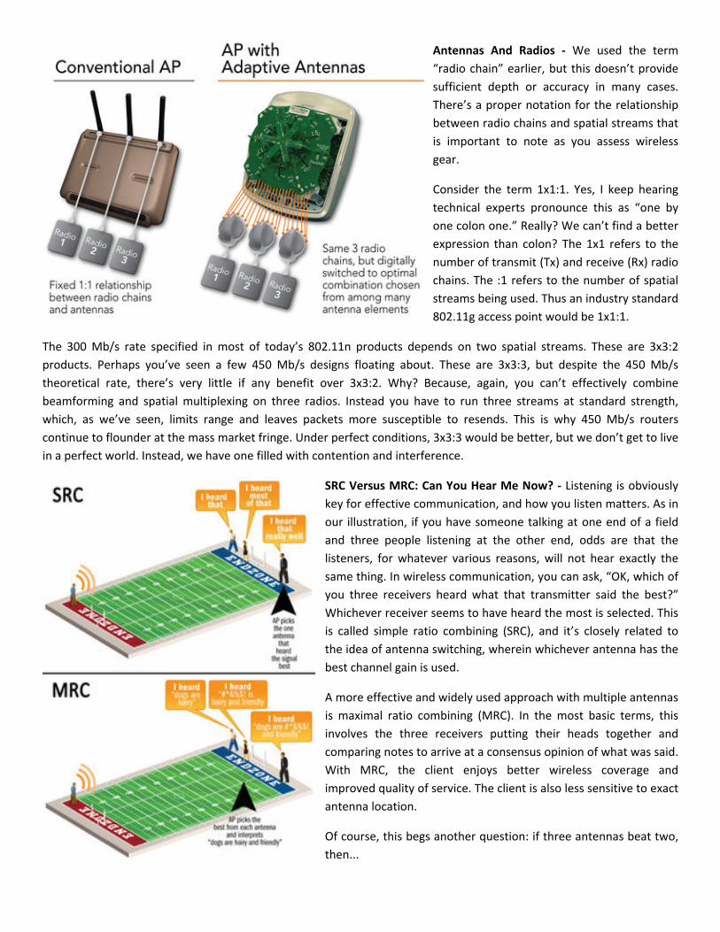
Antennas And Radios ‐ We used the term
“radio chain” earlier, but this doesn’t provide
sufficient depth or accuracy in many cases.
There’s a proper notation for the relationship
between radio chains and spatial streams that
is important to note as you assess wireless
gear.
Consider the term 1x1:1. Yes, I keep hearing
technical experts pronounce this as “one by
one colon one.” Really? We can’t find a better
expression than colon? The 1x1 refers to the
number of transmit (Tx) and receive (Rx) radio
chains. The :1 refers to the number of spatial
streams being used. Thus an industry standard
802.11g access point would be 1x1:1.
The 300 Mb/s rate specified in most of today’s 802.11n products depends on two spatial streams. These are 3x3:2
products. Perhaps you’ve seen a few 450 Mb/s designs floating about. These are 3x3:3, but despite the 450 Mb/s
theoretical rate, there’s very little if any benefit over 3x3:2. Why? Because, again, you can’t effectively combine
beamforming and spatial multiplexing on three radios. Instead you have to run three streams at standard strength,
which, as we’ve seen, limits range and leaves packets more susceptible to resends. This is why 450 Mb/s routers
continue to flounder at the mass market fringe. Under perfect conditions, 3x3:3 would be better, but we don’t get to live
in a perfect world. Instead, we have one filled with contention and interference.
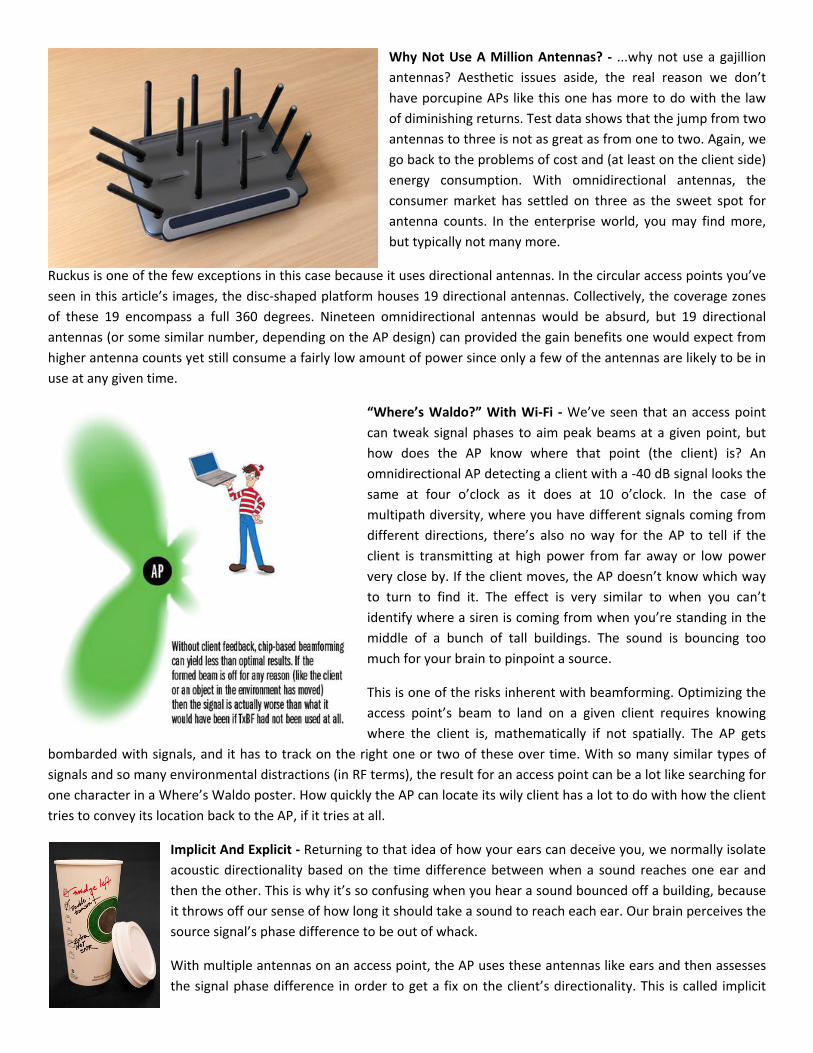
SRC Versus MRC: Can You Hear Me Now? ‐ Listening is obviously
key for effective communication, and how you listen matters. As in
our illustration, if you have someone talking at one end of a field
and three people listening at the other end, odds are that the
listeners, for whatever various reasons, will not hear exactly the
same thing. In wireless communication, you can ask, “OK, which of
you three receivers heard what that transmitter said the best?”
Whichever receiver seems to have heard the most is selected. This
is called simple ratio combining (SRC), and it’s closely related to
the idea of antenna switching, wherein whichever antenna has the
best channel gain is used.
A more effective and widely used approach with multiple antennas
is maximal ratio combining (MRC). In the most basic terms, this
involves the three receivers putting their heads together and
comparing notes to arrive at a consensus opinion of what was said.
With MRC, the client enjoys better wireless coverage and
improved quality of service. The client is also less sensitive to exact
antenna location.
Of course, this begs another question: if three antennas beat two,
then...
Why Not Use A Million Antennas? ‐ ...why not use a gajillion
antennas? Aesthetic issues aside, the real reason we don’t
have porcupine APs like this one has more to do with the law
of diminishing returns. Test data shows that the jump from two
antennas to three is not as great as from one to two. Again, we
go back to the problems of cost and (at least on the client side)
energy consumption. With omnidirectional antennas, the
consumer market has settled on three as the sweet spot for
antenna counts. In the enterprise world, you may find more,
but typically not many more.
Ruckus is one of the few exceptions in this case because it uses directional antennas. In the circular access points you’ve
seen in this article’s images, the disc‐shaped platform houses 19 directional antennas. Collectively, the coverage zones
of these 19 encompass a full 360 degrees. Nineteen omnidirectional antennas would be absurd, but 19 directional
antennas (or some similar number, depending on the AP design) can provided the gain benefits one would expect from
higher antenna counts yet still consume a fairly low amount of power since only a few of the antennas are likely to be in
use at any given time.
“Where’s Waldo?” With Wi‐Fi ‐ We’ve seen that an access point
can tweak signal phases to aim peak beams at a given point, but
how does the AP know where that point (the client) is? An
omnidirectional AP detecting a client with a ‐40 dB signal looks the
same at four o’clock as it does at 10 o’clock. In the case of
multipath diversity, where you have different signals coming from
different directions, there’s also no way for the AP to tell if the
client is transmitting at high power from far away or low power
very close by. If the client moves, the AP doesn’t know which way
to turn to find it. The effect is very similar to when you can’t
identify where a siren is coming from when you’re standing in the
middle of a bunch of tall buildings. The sound is bouncing too
much for your brain to pinpoint a source.
This is one of the risks inherent with beamforming. Optimizing the
access point’s beam to land on a given client requires knowing
where the client is, mathematically if not spatially. The AP gets
bombarded with signals, and it has to track on the right one or two of these over time. With so many similar types of
signals and so many environmental distractions (in RF terms), the result for an access point can be a lot like searching for
one character in a Where’s Waldo poster. How quickly the AP can locate its wily client has a lot to do with how the client
tries to convey its location back to the AP, if it tries at all.
Implicit And Explicit ‐ Returning to that idea of how your ears can deceive you, we normally isolate
acoustic directionality based on the time difference between when a sound reaches one ear and
then the other. This is why it’s so confusing when you hear a sound bounced off a building, because
it throws off our sense of how long it should take a sound to reach each ear. Our brain perceives the
source signal’s phase difference to be out of whack.
With multiple antennas on an access point, the AP uses these antennas like ears and then assesses
the signal phase difference in order to get a fix on the client’s directionality. This is called implicit
beamforming. The beamform is directed to a course derived implicitly from the detected signal phase. However, the AP
can be confused by odd signal bounces just like your brain can. This confusion can be compounded by differences in the
uplink and downlink paths.
With explicit beamforming, the client says exactly what it wants, just as if it was placing a complicated espresso order.
The client makes requests regarding transmit phase, power, and other factors relative to its current circumstances in the
radio environment. The results are far more accurate and effective than implicit beamforming. So what’s the catch?
Nobody supports explicit beamforming, at least not in today’s client devices. Both implicit and explicit methods must be
built into the Wi‐Fi chipset. Hopefully, explicit support will arrive soon.
Polarization ‐ On top of all the other issues we’ve
encountered with wireless communications so far, we can
add polarization to the list. Polarization is a bigger deal
than many people suspect, and I had the chance to
witness its effects first‐hand with an iPad 2. But first, the
theory...
You probably know that light travels in waves, and all
waveforms have a directional orientation. This is why
polarized sunglasses work so well. Light that reflects off
of the road or snow and into your eyes tends to be
polarized along a horizontal orientation, parallel to the
ground. The polarized filter coating in sunglasses is
oriented in a vertical orientation. Think of the waveform
as a big, long piece of cardboard you’re trying to slide
through window blinds. If you’re holding the cardboard
horizontally, and it encounters vertical blinds, the cardboard will be blocked. If the blinds are horizontal, like Venetian
blinds, then the cardboard can slide through unimpeded. Sunglasses are designed to cut glare in particular, which has a
horizontal orientation.
Back to Wi‐Fi. When a signal emits from an antenna, it carries the polarization orientation of that antenna. So if the AP is
sitting on a table and the emitting antenna is pointing straight up, then the emitted waveform will have a vertical
orientation. It follows that the receiving antenna, if it’s going to have the best reception possible, should also have a
vertical orientation. The reverse is also true—the receiving AP should have antenna(s) in polarization alignment with the
sending client. The further out of polarization alignment the antennas are, the worse the signal reception. The good
news here is that most routers and access points have moveable antennas that allow users to suit their positioning to
the best possible client reception, much like bunny ears on TV sets. The bad news is that because so few people
understand the principles of how their Wi‐Fi gear uses polarization, hardly anyone performs this orientation
optimization.
With all of that said, as you look at the above illustration, you’ll see that the access point is emitting both a horizontal
(top) and a vertical signal waveform to the iPad 2 client. Which orientation results in better reception quality and
performance? That depends on how many antennas are operating within the client and the orientation of those
antennas.
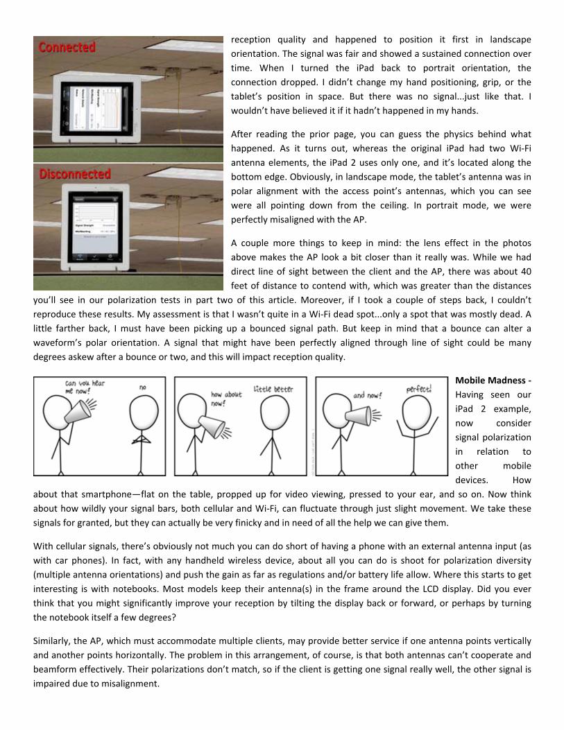
Taking A Bad Bounce ‐ Now, about that first‐hand experience I had with iPad 2 polarization. I was standing just about
where the camera was when the above picture was taken. You can see the Aruba access point to which I was connected
hanging from the ceiling in the background. I held the tablet up by its corners with two hands. I was simply looking for
reception quality and happened to position it first in landscape
orientation. The signal was fair and showed a sustained connection over
time. When I turned the iPad back to portrait orientation, the
connection dropped. I didn’t change my hand positioning, grip, or the
tablet’s position in space. But there was no signal...just like that. I
wouldn’t have believed it if it hadn’t happened in my hands.
After reading the prior page, you can guess the physics behind what
happened. As it turns out, whereas the original iPad had two Wi‐Fi
antenna elements, the iPad 2 uses only one, and it’s located along the
bottom edge. Obviously, in landscape mode, the tablet’s antenna was in
polar alignment with the access point’s antennas, which you can see
were all pointing down from the ceiling. In portrait mode, we were
perfectly misaligned with the AP.
A couple more things to keep in mind: the lens effect in the photos
above makes the AP look a bit closer than it really was. While we had
direct line of sight between the client and the AP, there was about 40
feet of distance to contend with, which was greater than the distances
you’ll see in our polarization tests in part two of this article. Moreover, if I took a couple of steps back, I couldn’t
reproduce these results. My assessment is that I wasn’t quite in a Wi‐Fi dead spot...only a spot that was mostly dead. A
little farther back, I must have been picking up a bounced signal path. But keep in mind that a bounce can alter a
waveform’s polar orientation. A signal that might have been perfectly aligned through line of sight could be many
degrees askew after a bounce or two, and this will impact reception quality.
Mobile Madness ‐
Having seen our
iPad 2 example,
now consider
signal polarization
in relation to
other mobile
devices. How
about that smartphone—flat on the table, propped up for video viewing, pressed to your ear, and so on. Now think
about how wildly your signal bars, both cellular and Wi‐Fi, can fluctuate through just slight movement. We take these
signals for granted, but they can actually be very finicky and in need of all the help we can give them.
With cellular signals, there’s obviously not much you can do short of having a phone with an external antenna input (as
with car phones). In fact, with any handheld wireless device, about all you can do is shoot for polarization diversity
(multiple antenna orientations) and push the gain as far as regulations and/or battery life allow. Where this starts to get
interesting is with notebooks. Most models keep their antenna(s) in the frame around the LCD display. Did you ever
think that you might significantly improve your reception by tilting the display back or forward, or perhaps by turning
the notebook itself a few degrees?
Similarly, the AP, which must accommodate multiple clients, may provide better service if one antenna points vertically
and another points horizontally. The problem in this arrangement, of course, is that both antennas can’t cooperate and
beamform effectively. Their polarizations don’t match, so if the client is getting one signal really well, the other signal is
impaired due to misalignment.
If Rx antennas are only looking for waveforms in one orientation, that's a recipe for failure. This is why it’s important to
have more orientations on the receiving end. If you had two receiving antennas, one vertical and one horizontal, and
two vertical Tx, you would only receive one stream well.
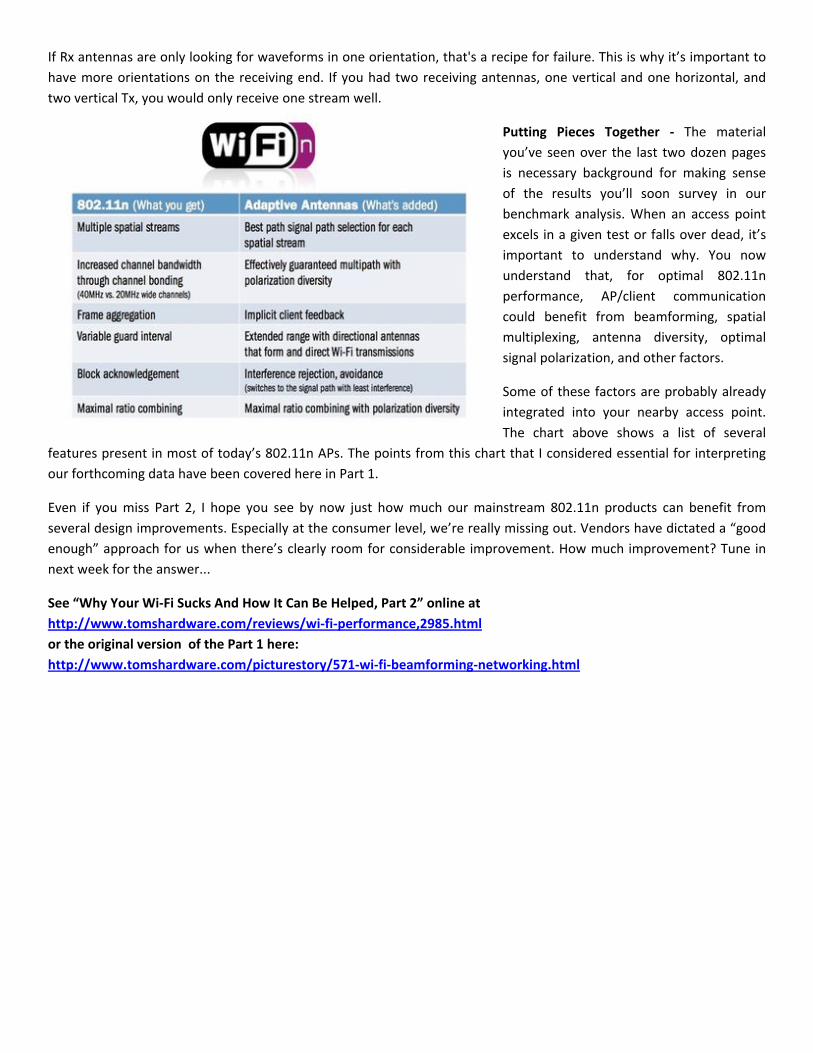
Putting Pieces Together ‐ The material
you’ve seen over the last two dozen pages
is necessary background for making sense
of the results you’ll soon survey in our
benchmark analysis. When an access point
excels in a given test or falls over dead, it’s
important to understand why. You now
understand that, for optimal 802.11n
performance, AP/client communication
could benefit from beamforming, spatial
multiplexing, antenna diversity, optimal
signal polarization, and other factors.
Some of these factors are probably already
integrated into your nearby access point.
The chart above shows a list of several
features present in most of today’s 802.11n APs. The points from this chart that I considered essential for interpreting
our forthcoming data have been covered here in Part 1.
Even if you miss Part 2, I hope you see by now just how much our mainstream 802.11n products can benefit from
several design improvements. Especially at the consumer level, we’re really missing out. Vendors have dictated a “good
enough” approach for us when there’s clearly room for considerable improvement. How much improvement? Tune in
next week for the answer...
See “Why Your Wi‐Fi Sucks And How It Can Be Helped, Part 2” online at