Willingness to Accept Equals Willingness to Pay for …ftp.iza.org/dp6816.pdfA revised version may...

DI

SC

US

SI

ON

P

AP

ER

S

ER

IE

S

Forschungsinstitut zur Zukunft der ArbeitInstitute for the Study of Labor

Willingness to Accept Equals Willingness to Pay for Labor Market Estimates of the Value of Statistical Life

IZA DP No. 6816

August 2012

Thomas J. KniesnerW. Kip ViscusiJames P. Ziliak

Willingness to Accept Equals Willingness to Pay for Labor Market

Estimates of the Value of Statistical Life

Thomas J. Kniesner Claremont Graduate University,

Syracuse University and IZA

W. Kip Viscusi Vanderbilt University

and NBER

James P. Ziliak University of Kentucky

Discussion Paper No. 6816 August 2012

IZA

P.O. Box 7240 53072 Bonn

Germany

Phone: +49-228-3894-0 Fax: +49-228-3894-180

E-mail: [email protected]

Any opinions expressed here are those of the author(s) and not those of IZA. Research published in this series may include views on policy, but the institute itself takes no institutional policy positions. The Institute for the Study of Labor (IZA) in Bonn is a local and virtual international research center and a place of communication between science, politics and business. IZA is an independent nonprofit organization supported by Deutsche Post Foundation. The center is associated with the University of Bonn and offers a stimulating research environment through its international network, workshops and conferences, data service, project support, research visits and doctoral program. IZA engages in (i) original and internationally competitive research in all fields of labor economics, (ii) development of policy concepts, and (iii) dissemination of research results and concepts to the interested public. IZA Discussion Papers often represent preliminary work and are circulated to encourage discussion. Citation of such a paper should account for its provisional character. A revised version may be available directly from the author.

mailto:[email protected]

IZA Discussion Paper No. 6816 August 2012

ABSTRACT

Willingness to Accept Equals Willingness to Pay for Labor Market Estimates of the Value of Statistical Life

Our research clarifies the conceptual linkages among willingness to pay for additional safety, willingness to accept less safety, and the value of statistical life (VSL). We present econometric estimates that in the important case of workers’ decisions concerning exposure to fatal injury risk there is no statistically significant divergence between willingness to accept and willingness to pay. Our focal result contrasts with the literature documenting a considerable asymmetry in tradeoff rates for increases and decreases in risk. An important implication for policy is that it is reasonable to use labor market estimates of VSL as a measure of the willingness to pay for additional safety. JEL Classification: C23, I10, J17, J28, K00 Keywords: willingness to pay, willingness to accept, value of statistical life, VSL, CFOI,

panel data, PSID Corresponding author: Thomas J. Kniesner Center for Policy Research Syracuse University 426 Eggers Hall Syracuse, NY 13244-1020 USA E-mail: [email protected]

mailto:[email protected]

1

1. Introduction

The fundamental principle for valuing the benefits of government policies is society’s

willingness to pay for the policy effects. In the case of regulations and other government policies

that reduce fatal injury risks, the policy impact to be valued is the expected number of lives that

will be saved by the policy. The standard measure of the willingness-to-pay value is the tradeoff

rate between money and fatal injury risks, or what is known as the value of statistical life (VSL).

Here we explicate the connections among VSL as willingness to pay for additional safety or

willingness to accept less safety and present estimates that there is no significant divergence

between willingness to accept and willingness to pay in the important case of the decisions

workers make concerning exposure to fatal injury risk.

The practice throughout the U.S. Federal government for estimating the VSL to be used

in benefit assessments is to rely principally on labor market estimates of VSL based on workers’

wage-risk tradeoffs.1 Labor market estimates capture the compensating differential that workers

require to incur job risks as compared to a risk-free job. Consequently, from the vantage point of

a model in which workers are comparing a hypothetical baseline risk-free job with a risky job,

the estimated wage-risk tradeoffs are not estimates of willingness to pay (WTP) for a decrease in

risk but rather are measures of willingness to accept (WTA) for the increase in risk associated

with taking the hazardous job compared to the safe alternative. Given the assumptions of

standard hedonic labor market models, the local rates of tradeoff for WTA and WTP are identical

for very small changes in risk. Consequently, the use of labor market estimates of VSL as a WTP

measure in policy applications is reasonable.

1 See U.S. Office of Management and Budget Circular A-4, Regulatory Analysis (Sept. 17, 2003), which is available at http://www.whitehouse.gov/omb/circulars/a004/a-4.pdf; U.S. Dept. of Transportation, Office of the Assistant Secretary for Transportation Policy, “Memorandum: Treatment of the Economic Value of Statistical Life in Departmental Analyses,” http://ostpxweb.gov.policy/reports/080205.htm; and U.S. Environmental Protection Agency, “Valuing Mortality Risk Reductions for Environmental Policy: A White Paper,” SAB Review Draft, 2010.

2

Various models of the rationality of individual choice have hypothesized that there may,

however, be important status quo effects that can generate a spread between WTA and WTP

values. In the Kahneman and Tversky (1979) prospect theory model, utility levels are based on

changes in wealth rather than on levels of wealth, and people are assumed to be much more

averse to a loss in money than would be indicated by their valuation of an increase in money.

Thus, there is a kink in utility functions associated with a shift in marginal utility values at the

current wealth level. Numerous other models have incorporated similar kinds of reference point

effects in which the tradeoff rate for a decrease in some attribute is quite different than for a

comparable increase.

A wide body of literature involving economic experiments and stated preference studies

has documented a substantial discrepancy between WTA and WTP values for the same

commodity. The meta-analysis by Horowitz and McConnell (2002) reviewed a large set of

studies over a wide range of commodities, including environmental outcomes and real goods,

and found an average of the mean values of WTA/WTP of 7.2. If VSL estimates are viewed as

WTA values rather than WTP and also are characterized by a similar WTA/WTP ratio, then

meta-analysis estimates of the median labor market estimates of VSL of $7 million in $2000

(Viscusi and Aldy, 2003) should be reduced to $1 million in order to reflect the value of WTP

rather than WTA. Such a change in VSL levels would have a profound effect on benefit

estimates for government regulations and on which policies pass a benefit-cost test. However, no

studies to date have explored the discrepancy between WTA and WTP values in the risky job

choice situation.

The WTA/WTP gap for labor market decisions may be different than that identified in

experimental studies. First, job choices involve repeated decisions for which the individual is

3

able to acquire information such as that provided by hazard warnings, observations of various

workplace signals of injury risks such as lax safety standards, and personal experience with

whether the job poses a risk of injury. The WTA/WTP gap is related to the family of influences

associated with endowment effects. Evidence for endowment effects indicates that experience

with a good may affect the existence and strength of the asymmetry between buying and selling

prices (List, 2003). Second, while some experimental studies use actual commodities rather than

hypothetical payoffs, the stakes involved in life-or-death risky job decisions are much greater.

Even on an expected value basis, the magnitude of the typical VSL estimate multiplied by the

average job fatal injury risk is roughly two orders of magnitude larger than the stakes in any

related experiments dealing with reference dependence effects. Whether greater stakes increase

or decrease the WTA/WTP discrepancy based on theory is unclear, but the importance of the

decision and the incentives to think carefully about one’s choices are greater for repeated

exposures to fatal injury risks.2 Third, risks of death on the job differ from commodities in most

of the previous literature in that life and health affect utility functions in a manner that cannot be

treated as a monetary equivalent.

How one should characterize a situation of compensating differentials depends on the

reference point so that treating labor market estimates of VSL as always being a WTA value is

not correct. The categorization of labor market estimates as a WTA amount based on an

economic model in which workers face a hypothetical choice between a risk-free job and a risky

job is overly simplistic and ignores the shifting nature of the worker’s reference point in actual

job choice situations. Whether labor market estimates of VSL reflect a WTP or WTA amount

depends on how the worker’s current job differs from the worker’s baseline situation, which is

2 For minor health effects that do not reduce the marginal utility of income, Chilton et al. (2012) report stated preference evidence indicating a narrowing of the WTA/WTP gap for more minor health effects.

4

unlikely to involve risk-free employment. The status quo for the worker is being continuously

redefined as the worker changes jobs over the lifetime. If the worker accepts the compensating

differential to move from the current job to a higher risk job, the estimated wage-risk tradeoff

rate is a WTA measure of VSL. However, if the worker moves from a riskier job to a lower risk

job with a decreased risk differential, then the wage-risk tradeoff rate is a WTP measure even

though the new job is not risk-free and will generate a compensating differential compared to a

zero risk job.

Use of panel data to examine such job changes can potentially provide insight into

whether there is a discrepancy between WTA and WTP measures of VSL. However, with but a

few exceptions (Brown 1980, Villanueva 2007, Schaffner and Spengler 2010, and Kniesner,

Viscusi, Woock, and Ziliak 2012) that have used panel data to examine VSL, all labor market

estimates have focused on cross-sectional evidence. And no panel study to date has examined

whether there is any difference in tradeoff rates in the WTA and WTP situations. Here we use

data from the Panel Study of Income Dynamics (PSID) in conjunction with very refined

measures of fatal injury risk to explore possible asymmetries in VSL based on whether the job

change should be viewed as a WTA or WTP situation.

To summarize our research, first we provide a theoretical framework in which there are

reference point effects whereby workers can be particularly averse to changes on dimensions that

make them worse off. There could be a reference effect associated with either a decrease in

wages or an increase in the fatal injury risk. The models incorporate the several possible

reference effects an otherwise standard model of labor market estimates of VSL and show that

the ratio WTA/WTP will exceed 1.0 if either of the reference effects is influential. We then use

the PSID to test whether there is such a reference effect(s) generating a difference between WTA

5

and WTP. By focusing on job changers, we are able to distinguish situations that should be

reflective of the WTA and WTP situations. There is no statistically significant difference in VSL

across the two groups. Though the point estimates of VSL are sometimes higher for risk

increases than for risk decreases, the WTA and WTP values for labor market estimates of VSL

are not significantly different.

2. Compensating Differentials with Reference Effects

The focus of our empirical analysis is on workers in risky occupations who change jobs.

We take as given the standard aspects of the hedonic labor market models. Workers are choosing

jobs from a market opportunities locus, which is the outer envelope of firms’ market offer

curves. Available jobs are associated with a wage rate and an objective risk measure, which in

our empirical analysis we will equate with the fatal injury rate for the worker’s industry-

occupation cell. This locus offers a higher wage rate for jobs posing greater risk, so that increases

in job risk are associated with greater pay and decreases in job risks are associated with smaller

compensating differentials. For simplicity assume that there are no transactions costs to changing

jobs.

2.1. Wage-Risk Tradeoffs

Let the worker’s initial job be characterized by a fatal injury risk p0 and a wage w0. This

position gives the worker the highest expected utility level of all the available jobs on the market

opportunities locus. The worker has an indirect utility function u(w), where u′ > 0 and u″ ≤ 0.

Levels of wealth and other income are subsumed in the functional form of u(w). If the worker is

killed on the job, the utility level is zero. The expected utility v(p0, w0) of the base case job

situation is given by

).u(w )p (1 = ) w,v(p 0000 (1)

6

If the worker’s experiences on the job are favorable, the position becomes increasingly

attractive relative to other positions, and there is no incentive for the worker to quit. If the worker

has an unfavorable experience, such as observing risky job conditions, the posterior probability

of a fatal accident is 0*0 pp .3 Thus, the worker with an adverse experience may believe that job

is more dangerous than given by the average objective risk value.

Now that the attractiveness of the initial job has declined, for the second and final period

in the model let the worker consider some alternative job from the available opportunities set.

Let the worker consider changing jobs to a position with a fatal injury rate p1 and wage w1. For

the alternative position to be desirable compared to the initial job the worker’s reservation wage

for the new job must satisfy

, ) w, v(p= )u(w )p (1 = ) w,v(p 11110*0 (2)

where )w,v(p 0*0 equals some constant value. If there are no reference point effects involving the

wage or the fatal injury risk, whether the job change involves an increase in risk for more pay or

a decrease in risk for less pay does not enter the expected utility calculation.

By implicit differentiation of v(p1, w1), one can calculate the reservation wage-risk

tradeoff rate for the new job, or

)(wu)p(1

)(wu

v

v

p

w

11

1

w

p

1

1

1

1

, (3)

where this expression is defined as the VSL. In the case of a new job involving a higher wage

rate for greater risk, w1/p1 is a willingness-to-accept measure. In the standard situation with

no reference point effects,

3 If workers have a beta distribution of assessed fatal injury risks with γ being the informational content of the prior and p0 reflecting the probability of an adverse outcome, the posterior probability of *

0p that prevails after observing

information equivalent to one unfavorable trial outcome is (γp0 + 1)/( γ +1) > p0.

7

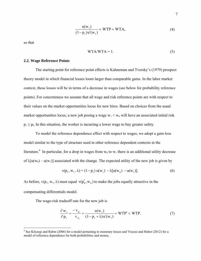
WTA,WTP)(wu)p(1

)(wu

11

1

(4)

so that

WTA/WTA = 1. (5)

2.2. Wage Reference Points

The starting point for reference point effects is Kahneman and Tversky’s (1979) prospect

theory model in which financial losses loom larger than comparable gains. In the labor market

context, these losses will be in terms of a decrease in wages (see below for probability reference

points). For concreteness we assume that all wage and risk reference points are with respect to

their values on the market opportunities locus for new hires. Based on choices from the usual

market opportunities locus, a new job posing a wage w1 < w0 will have an associated initial risk

p1 ≤ p0. In this situation, the worker is incurring a lower wage to buy greater safety.

To model the reference dependence effect with respect to wages, we adopt a gain-loss

model similar to the type of structure used in other reference dependent contexts in the

literature.4 In particular, for a drop in wages from w0 to w1 there is an additional utility decrease

of λ[u(w0) – u(w1)] associated with the change. The expected utility of the new job is given by

1 1 1 1 0 1v(p , w , λ) = (1 p ) u(w ) λ[u(w ) u(w )]. (6)

As before, v(p1, w1, λ) must equal )w,v(p 0*0 to make the jobs equally attractive in the

compensating differentials model.

The wage-risk tradeoff rate for the new job is

WTP.PWT)(wuλ)p(1

)(wu

v

v

p

w

11

1

w

p

1

1

1

1

(7)

4 See Kőszegi and Rabin (2006) for a model pertaining to monetary losses and Viscusi and Huber (2012) for a model of reference dependence for both probabilities and money.

8

The reference wage effect serves to lower the value of WTP as incurring a wage cut for greater

safety is less attractive. Because the wage reference effect influences the value of WTP but not

WTA, the ratio

1.p1

λp1

)(wu

λ)p(1

)(wu)p(1

)(wu

PWT

WTA

1

1

1

1

11

1

(8)

The ratio of WTA to WTP′ exceeds 1 since WTP has been reduced by the reference wage effect,

while WTA is unaffected.

2.3. Probability Reference Points

Suppose that the reference point of consequence is not with respect to wages but rather

workers’ unwillingness to move to a job with greater objective risk value p1 > p0. To model this

case, we assume a reference utility loss of µ(p1 – p0) associated with job changes that involve an

increase in the worker’s objective risk level. The expected utility of the new job is consequently

).p µ(p )u(w )p (1 = µ) , w,v(p 011111 (9)

Assessment of the wage-risk tradeoff yields the result that

WTA.AWT)(wu)p(1

μ)(wu

v

v

p

w

11

1

w

p

1

1

1

1

(10)

In calculating the ratio of willingness-to-accept to willingness-to-pay, it is WTP that is the

pertinent value rather than WTP′ since the wage rate is not declining in this instance. As a result,

for job changes involving more pay for greater risk,

1.)(wu

μ)(wu

WTP

AWT

1

1

(11)

2.4. Both Monetary and Probability Reference Points

Any job change that is equally attractive as the worker’s current position will trigger only

one reference point effect even if both potentially may be influential. For p1 < p0 and w1 < w0,

9

there will be a wage reference effect making WTP′ < WTP. For p1 > p0 and w1 > w0, there is a

probability reference effect leading to WTA′ > WTA. Both reference point effects will not result

from the same job change. Irrespective of whether it is the wage reference point or fatal injury

risk reference point that comes into play, willingness to accept will exceed willingness to pay.

3. Data and Regression Variables

When examining whether labor market decisions display WTA = WTP our primary data

source is the 1993-2001 waves of the Panel Study of Income Dynamics (PSID), which provides

worker-level data on wages, industry, occupation, and key personal characteristics. The

particular PSID data that we use are the random Survey Research Center sample of male heads

of households ages 18-65 who (a) worked for an hourly or salary pay during the previous

calendar year, (b) were not permanently disabled or institutionalized, (c) were not in agriculture

or the armed forces, (d) had a real hourly wage greater than $2 and less than $100, and (e) had no

missing data on wages, education, region, industry, and occupation.

Beginning in 1997 the PSID changed to interviewing every other year. To have

consistently spaced survey responses we use data from the 1993, 1995, 1997, 1999, and 2001

waves. We do not require workers to be present for the entire sample period; we have an

unbalanced panel where we take missing values as random events.5 Our sample inclusion

conditions resulted in 2,036 men and 6,625 person years. About 40% of the men appear on all

five waves (covering nine years) and another 25% are present for four waves.

The dependent variable in our regressions is the hourly wage rate. We deflate the nominal

wage by the personal consumption expenditure deflator for the 2001 base year. We then take the

5 When there is time-invariant non-random attrition the differenced data models we use will remove it along with other latent time-invariant factors (Ziliak and Kniesner 1998).

10

natural log of the real wage rate to downplay the influence of outliers as well as for ease of

comparison with others’ estimates.

The focal regressor in our research is the fatal injury rate of the worker’s two-digit

industry by one-digit occupation group, which we denote as . We created the 720 industry-

occupation groups as the intersections of 72 two-digit SIC code industries and the 10 one-digit

occupational groups. We constructed our workers’ fatal injury risk variable using proprietary

U.S. Bureau of Labor Statistics data from the Census of Fatal Occupational Injuries (CFOI) for

1992-2002.6 The CFOI provides the most comprehensive and accurate inventory available of all

work-related fatalities in a given year.

It is important to emphasize that we construct two measures of fatal risk. The first uses

the number of fatalities in each industry-occupation cell in survey year t divided by the number

of employees for that industry-occupation cell in survey year t. The second measure uses a three-

year average of fatalities surrounding each PSID survey year (1992-1994 for the 1993 wave,

1994-1996 for the 1995 wave, and so on), divided by a similar three-year average of

employment. Both of our measures of the fatal injury risk time-vary because of changes in the

numerator and the denominator.

We expect there may be less measurement error in the three-year average fatal injury

rates relative to the annual rate because of the averaging process, which will reduce the influence

of random fluctuations in fatalities as well as mitigate the small sample problems that arise from

many narrowly defined job categories. Alternatively, the annual measure should be a more

pertinent measure of the risk in that particular survey year.

6 The fatal injury data we use can be obtained through a confidentiality agreement with the U.S. Bureau of Labor Statistics. How we construct our regressions’ fatal injury risk variable follows Viscusi (2004), which describes the procedures in more detail.

11

Kniesner, et al. (2012) show that the main source of variation identifying compensating

differentials for fatal injury risk comes from workers who switch industry-occupation cells over

time. That is, some changes in fatal injury risk occur because of within industry-occupation cell

changes and others occur because workers switch industry-occupation cells. Kniesner, et al. find

that the within-group variation is 8 times higher for job changers than job stayers, and thus job

changers are key to identifying compensating differentials. Thus, in our empirical models below

we focus on two types of job changers—those who ever switch industry/occupation over the

sample period, and the year that they switch. The latter group is a subset of the former. Appendix

A lists the means for both the annual and three-year fatal injury risk measures for the samples of

workers that ever change jobs or when they change jobs. The sample in Appendix A is for those

used in our first-difference regression models described below. The sample mean risks for the

annual measures for the two samples are 6.31/100,000 and 6.21/100,000, respectively. As

expected the variation in the annual measure exceeds that of the three-year average.

4. Econometric Estimates of WTA and WTP

For ease of presentation and discussion we suppress the coefficients other than those

involving fatal risk. Every regression model in what follows controls for a quadratic in age; years

of schooling; and indicators for marital status, union status, race, one-digit occupation, two-digit

industry, region, state, and year. The occupation and industry dummies account for the

substantial heterogeneity of jobs in different occupations and industries. Because there might

also be unmeasured differences in labor markets across states and regions that do not vary over

time we include the full set of state and region (nine Census divisions) fixed effects. Year

dummies control for common macroeconomic shocks. Finally, the standard errors that we report

are clustered by industry and occupation and are also robust to the relevant heteroskedasticity.

12

Note the first-difference baseline specifications automatically net out the influence of workers’

compensation, industry, and other job and personal characteristics that do not change over time.

Appendix A provides means of the regression variables for the three samples used in estimation.

4.1 Baseline Wage Equation Estimates

As we emphasize in Kniesner et al. (2012), it is crucial to control for latent worker

heterogeneity when estimating the compensating wage differentials, and thus we adopt the first-

difference transformation as a baseline because wages have been shown to be non-stationary.

Our baseline first-difference estimates use

∆ ∆ ∆ ∆ (12)

and appear in Column (1) of Tables 1 and 2. As noted above the estimates from equation (12)

address systematically both latent heterogeneity and possibly trended regressors as well as

measurement errors, but force WTA = WTP. Our focal estimates are converted to estimates of

VSL for ease of discussion and economic and policy relevance and are constructed as

100,000 , where we evaluate VSL at the mean wage and sample

mean hours from Appendix A.

Our baseline estimates of VSL in Tables 1 and 2 with WTA = WTP imposed are $7.0 and

$7.2 million, respectively, based on the annual fatal injury rate coefficient.7 Given such VSL

magnitudes, any influence of income effects on the WTA-WTP gap is negligible.8 Possible

(random) measurement errors in workplace hazard rates will attenuate the coefficient estimate,

and thus the measurement error effect from models with 3-year average fatal injury rates should

7 In Kniesner, et al. (2012) the estimated VSL from the pooled model that included job stayers is $6.6 million. While this is statistically the same as the pooled VSLs reported in Tables 1 and 2 here, the qualitatively lower point estimate results from dampened variation in industry/occupation fatal risk among job stayers. 8A worker moving to a riskier job that poses an additional 5/100,000 risk will receive an added wage premium of $350, which is 0.7% of average annual income. Based on estimates of the income elasticity of VSL (Viscusi and Aldy, 2003), the effect of such income changes on the VSL will be under 0.5%.

13

be reduced by permitting the fatal injury rate to capture a wider time interval. Compared to VSLs

for the annual risk measure, the estimated VSLs in Tables 1 and 2 are about 40 percent larger

when fatal injury risk is a three-year average.

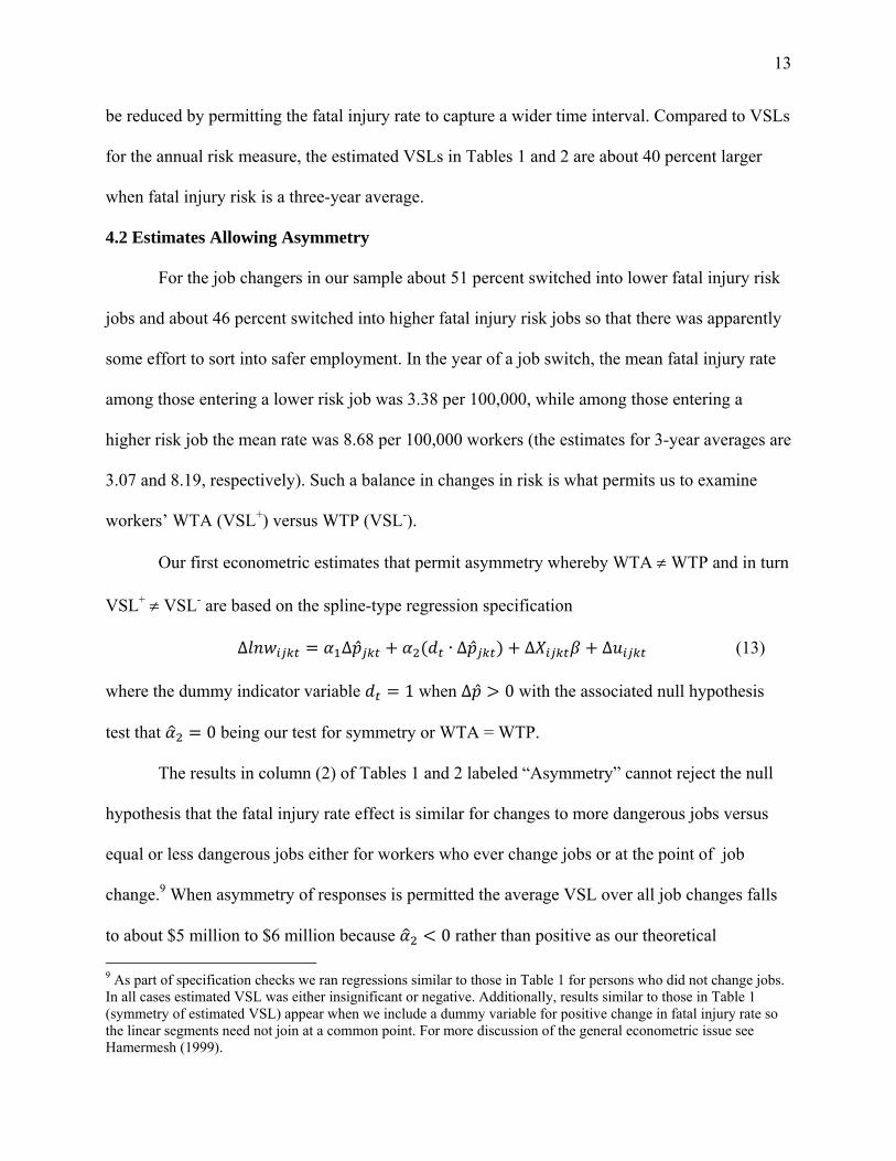
4.2 Estimates Allowing Asymmetry

For the job changers in our sample about 51 percent switched into lower fatal injury risk

jobs and about 46 percent switched into higher fatal injury risk jobs so that there was apparently

some effort to sort into safer employment. In the year of a job switch, the mean fatal injury rate

among those entering a lower risk job was 3.38 per 100,000, while among those entering a

higher risk job the mean rate was 8.68 per 100,000 workers (the estimates for 3-year averages are

3.07 and 8.19, respectively). Such a balance in changes in risk is what permits us to examine

workers’ WTA (VSL+) versus WTP (VSL-).

Our first econometric estimates that permit asymmetry whereby WTA WTP and in turn

VSL+ VSL- are based on the spline-type regression specification

∆ ∆ ∙ ∆ ∆ ∆ (13)

where the dummy indicator variable 1 when ∆ 0 with the associated null hypothesis

test that 0 being our test for symmetry or WTA = WTP.

The results in column (2) of Tables 1 and 2 labeled “Asymmetry” cannot reject the null

hypothesis that the fatal injury rate effect is similar for changes to more dangerous jobs versus

equal or less dangerous jobs either for workers who ever change jobs or at the point of job

change.9 When asymmetry of responses is permitted the average VSL over all job changes falls

to about $5 million to $6 million because 0 rather than positive as our theoretical

9 As part of specification checks we ran regressions similar to those in Table 1 for persons who did not change jobs. In all cases estimated VSL was either insignificant or negative. Additionally, results similar to those in Table 1 (symmetry of estimated VSL) appear when we include a dummy variable for positive change in fatal injury rate so the linear segments need not join at a common point. For more discussion of the general econometric issue see Hamermesh (1999).

14

discussion leads us to expect. Thus, our second econometric specification that permits

differences in WTA and WTP is to estimate the regression functions separately for when ∆ 0

(labeled “Increases in Fatal Risk” in Tables 1 and 2) versus ∆ 0 (labeled “Decreases in Fatal

Risk” in Tables 1 and 2). The model now relaxes the econometric restriction in equation (12) that

the only difference in wage processes determining WTA and WTP comes from the fatal risk

coefficient, whiles the theoretical discussion around equations (8) and (11) consider more

broadly differences in utility functions. In columns (3) and (4) of Tables 1 and 2 we find

WTA > WTP as predicted by the reference point effect models, but we cannot reject the null

hypothesis that WTA and WTP are statistically the same.

4.3 Estimates Allowing Asymmetry and Selection Effects

In an underappreciated paper Solon (1986) develops the reference point effect result as a

statistical argument involving heterogeneity of preferences among job changers in a panel data

regression model correcting for latent time-invariant heterogeneity. In particular, suppose that

workers who switch to more dangerous jobs require a large wage increase to accept a new job

that is more dangerous but workers who seek a safer job do not accept a safer job if it is

accompanied by much of a wage cut. The result will be an estimated hedonic locus in a panel

data set that is driven by worker selection effects that produce the result WTA > WTP.

Consequently, in our empirical work we also attempt to control for worker-specific selection

effects in estimating WTA versus WTP based on labor market pairings of risk and wages.

Possible selection effects just discussed lead us to develop an interactive factor model as

described in Bai (2009), which for wage levels here is

with (14)

0, (15)

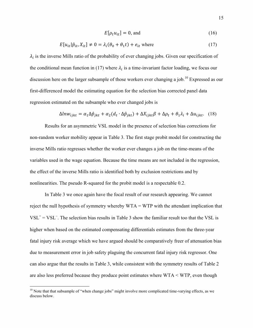
15

0, and (16)

| , 0 where (17)

is the inverse Mills ratio of the probability of ever changing jobs. Given our specification of

the conditional mean function in (17) where is a time-invariant factor loading, we focus our

discussion here on the larger subsample of those workers ever changing a job.10 Expressed as our

first-differenced model the estimating equation for the selection bias corrected panel data

regression estimated on the subsample who ever changed jobs is

∆ ∆ ∙ ∆ ∆ Δ ∆ . (18)

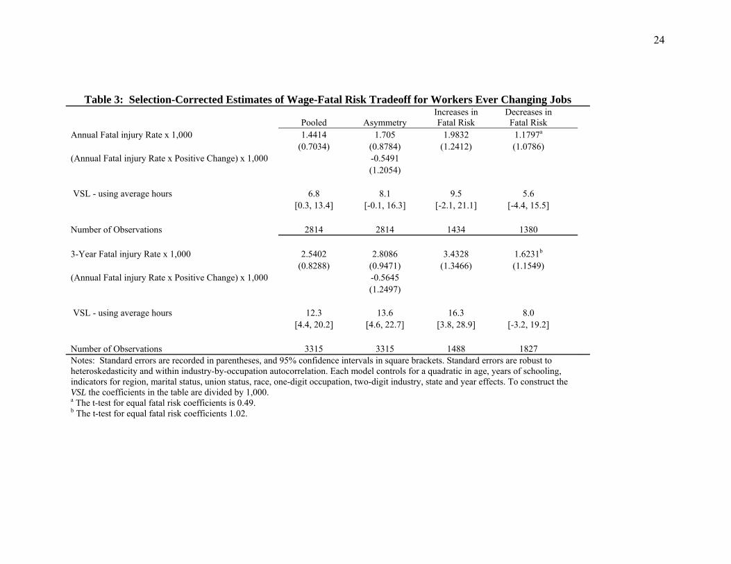
Results for an asymmetric VSL model in the presence of selection bias corrections for

non-random worker mobility appear in Table 3. The first stage probit model for constructing the

inverse Mills ratio regresses whether the worker ever changes a job on the time-means of the

variables used in the wage equation. Because the time means are not included in the regression,

the effect of the inverse Mills ratio is identified both by exclusion restrictions and by

nonlinearities. The pseudo R-squared for the probit model is a respectable 0.2.

In Table 3 we once again have the focal result of our research appearing. We cannot

reject the null hypothesis of symmetry whereby WTA = WTP with the attendant implication that

VSL+ = VSL. The selection bias results in Table 3 show the familiar result too that the VSL is

higher when based on the estimated compensating differentials estimates from the three-year

fatal injury risk average which we have argued should be comparatively freer of attenuation bias

due to measurement error in job safety plaguing the concurrent fatal injury risk regressor. One

can also argue that the results in Table 3, while consistent with the symmetry results of Table 2

are also less preferred because they produce point estimates where WTA < WTP, even though

10 Note that that subsample of “when change jobs” might involve more complicated time-varying effects, as we discuss below.

16

the difference is insignificant. Thus, in columns (3) and (4) of Table 3 we estimate the models

separately for increases versus decreases in fatal injury risk, and obtain the qualitatively expected

result that WTA > WTP, but continue to fail to reject the null hypothesis that they are

statistically the same.

Previous research demonstrates that wage functions may have not only idiosyncratic

differences in levels but also idiosyncratic differences in wage growth (Lillard and Weiss 1978).

The specification in equation (18) admits this possibility via inclusion of the inverse Mills ratio.

However, the specification may be unduly restrictive in the structure of the growth process.

Indeed, the specification of the inverse Mills ratio as a function of the time-means of the

regressors is an adaptation of the Mundlak (1978) correlated random effects model applied to a

model in differences rather than levels. Much like first differences is less restrictive than the

Mundlak approach for a panel data model in levels, a double-difference model is less restrictive

than the Heckman-selection model in (18). To correct for wages that may not be difference

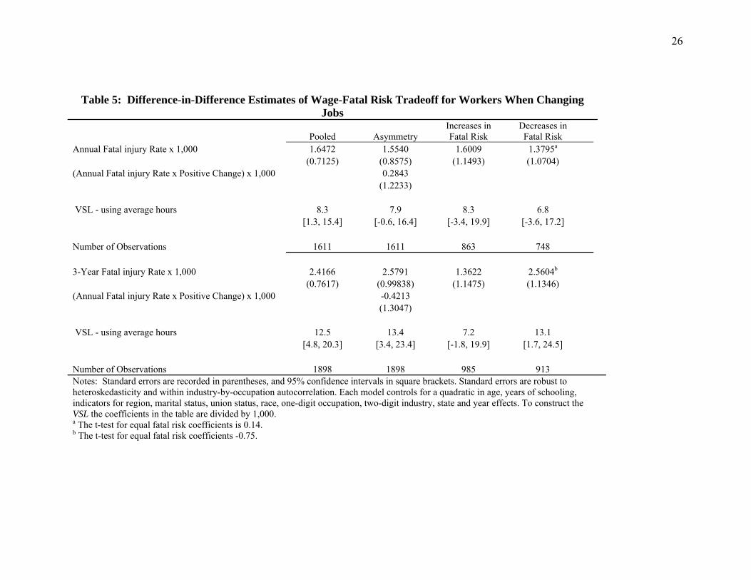
stationary we estimate a double-differenced version of (13) that is

Δ Δ ∙ Δ Δ Δ , (19)

where Δ Δ Δ , and is commonly known as the difference-in-differences operator.

The difference-in-differences estimates in Tables 4 and 5 are improvements over the

estimates in Tables 1 and 2 in the sense that in addition to symmetry the signs of both negative

and positive changes in fatal injury risk are now positive for the annual fatal injury specification

(because 0). The results in Tables 4 and 5 are also in the range of previous estimates of

VSL when symmetry is imposed ex ante. Again, we also estimate the difference-in-difference

models separately for increases versus decreases, and find that the theoretical result that WTA >

17

WTP does not hold qualitatively in all specifications, and statistically we cannot reject the null

that WTA = WTP.

5. Discussion

We emphasize that a key difference between our empirical research, which cannot reject

equality of WTA and WTP, and the extant estimated WTA > WTP literature is that the job

changers we study are moving either up or down from a job posing some quite small probability

of death to a job posing some other very small probability of death. We could in turn reasonably

hypothesize that the reference point effect-endowment effect type influence is less pronounced in

such situations in which the baseline is both probabilistic and involves probabilities on the order

of 1/25,000 to 2/25,000. By comparison, the effects may be more pronounced when the

probabilities involved are either 0 or 1. In Viscusi, Magat, and Huber (1987) there was a much

greater effect when the risk level became zero – a certainty premium, which is a possibility that

does not arise for safety risks.. All of the experiments with discrete goods such as mugs, soda,

candy bars, and pens take the probability of owning the good from 1 to 0. In situations where the

probability of ownership starts at 1, we might expect there to be more attachment to the good and

a stronger endowment effect than if the initial probability of ownership is very small.

Continuing with the link to the experimental literature, our results also can be interpreted

as consistent with the findings of Plott and Zeiler (2005), who ran experiments with lotteries and

mugs and found no divergence between WTA and WTP. They have several conjectures for their

findings that apply to our situation. Plott and Zeiler note that their subjects’ misperceptions

regarding the task can produce a WTA-WTP gap, which can be eliminated by extensively

training and instructing the subjects. Our workers deal with their decisions regularly so that they

do not misperceive the task. Second, in the experimental setting of Plott and Zeiler, people could

18

both buy and sell so that they became less attached to the good than in most endowment effects

experiments. Our workers too have the option of moving up or down in terms of risk so that they

are in effect buyers or sellers. Finally, the decision process in experimental settings is unfamiliar

to respondents, which can cause a WTA-WTP difference whereas the workers in our research are

in familiar job-choice contexts, which further makes sensible the core empirical result we present

here that the estimated WTA = WTP in the labor market concerning job-related risk of severe

injury.

Despite the absence of a statistically significant difference between WTA and WTP, in

seven of the ten comparisons the WTA value exceeded the WTP amount as predicted. The

average WTA amount is about 17% higher than the average WTP amount. However, even if

such discrepancies were to represent real differences, they would lead to only minor refinements

in the VSL that are well within the bounds of error. The more pressing concern stimulated by the

current literature is that the labor market estimate of the VSL might seriously overstate the

pertinent WTP amount for benefit assessments by almost an order of magnitude. It is clear based

on our results that there is not such discrepancy for labor market estimates of the VSL.

19

References

Bai, J. (2009). Panel data models with interactive fixed effects. Econometrica, 77(4), 1229-1279.

Brown, C. (1980). Equalizing differences in the labor market. Quarterly Journal of Economics,

94(1), 113–134.

Chilton, S., Jones-Lee, M., McDonald, R., & Metcalf, H. (2012). Does the WTA/WTP ratio

diminish as the severity of a health complaint is reduced? Testing for smoothness of the

underlying utility of wealth function. University of Newcastle working paper,

forthcoming in Journal of Risk and Uncertainty.

Greene, W. H. (2012). Econometric Analysis, Seventh Edition. Upper Saddle River, NJ: Pearson

Education, Publishing as Prentice Hall.

Hamermesh, D. S. (1999). The art of labormetrics. NBER Working Paper 6927.

Horowitz, J. K., & McConnell, K. E. (2002). A review of WTA/WTP studies. Journal of

Environmental Economics and Management, 44(3), 426–447.

Kahneman, D., & Tversky, A. (1979). Prospect theory: An analysis of decision under risk.

Econometrica, 47(2), 263–291.

Knetsch, J. L., & Tang, F-F. (2006). The context, or reference, dependence of economic values.

In M. Altman (Ed.), Handbook of Contemporary Behavioral Economics: Foundations

and Developments (423–440). New York, NY: M.E. Sharpe, Inc.

Kniesner, T. J., Viscusi, W. K., Woock, C., & Ziliak, J. P. (2012). The value of statistical life:

Evidence from panel data. Review of Economics and Statistics, 94(1), 74-87.

Kőszegi, B., & Rabin, M. (2006). A model of reference-dependent preferences. Quarterly

Journal of Economics, 121(4), 1133–1165.

20

Lillard, L. A. & Weiss, Y. (1979). Components of variation in panel earnings data: American

scientists 1960-70. Econometrica, 47(?), 437-454.

List, J. (2003). Does market experience eliminate market anomalies? Quarterly Journal of

Economics, 118, 41–71.

Mundlak, Y. (1978). On the pooling of time series and cross section data. Econometrica, 46(1),

69-85.

Plott, C. R. & Zeiler, K. (2005). The willingness to pay-willingness to accept gap, the

“endowment effect,” subject misperceptions, and experimental procedures for eliciting

valuations. American Economic Review, 95(3), 530-545.

Schaffner, S., & Spengler, H., (2010). Using job changes to evaluate the bias of value of

statistical life estimates. Resource and Energy Economics, 32(1), 15–27.

Solon, G. (1986). Bias in longitudinal estimation of wage gaps. NBER Working Paper 58.

Solon, G. (1989). The value of panel data in economic research. In D. Kasprzyk, D. Gregory, K.

Graham, and M. P. Singh (Eds.), Panel Surveys (486–496). Hoboken, NJ: Wiley.

Villanueva, E. (2007). Estimating compensating wage differentials using voluntary job changes:

Evidence from Germany. Industrial & Labor Relations Review, 60(4), 544-561.

Viscusi, W. K. (2004). The value of life: Estimates with risks by occupation and industry.

Economic Inquiry, 42(1), 29-48.

Viscusi, W. K., & Aldy, J. E. (2003). The value of a statistical life: A critical review of market

estimates throughout the world. Journal of Risk and Uncertainty, 27(1), 5–76.

Viscusi, W. K., & Huber, J. (2012). Reference-dependent valuations of risk: Why willingness-to-

accept exceeds willingness-to-pay. Journal of Risk and Uncertainty, 44(1), 19-44.

21

Viscusi, W. K., Magat, W., & Huber, J. (1987). An investigation of the rationality of consumer

valuations of multiple health risks. RAND Journal of Economics, 18(4), 465–479.

Ziliak, J. P. & Kniesner, T. J. (1998). The importance of sample attrition in life-cycle labor

supply estimation. Journal of Human Resources, 33(2), 507-530.

22

Table 1: First Difference Estimates of Wage-Fatal Risk Tradeoff for Workers Ever Changing Jobs

Pooled Asymmetry Increases in Fatal Risk

Decreases in Fatal Risk

Annual Fatal injury Rate x 1,000 1.4645 1.7482 2.1928 1.2316a

(0.6555) (0.8384) (1.1770) (1.0119) (Annual Fatal injury Rate x Positive Change) x 1,000 -0.5881

(1.1418)

VSL - using average hours 7.0 8.3 10.4 5.8 [0.9, 13.0] [0.5, 16.1] [-0.5, 21.4] [-3.6, 15.2]

Number of Observations 3035 3035 1558 1477

3-Year Fatal injury Rate x 1,000 2.105 2.2924 2.1221 1.7570b (0.7667) (0.8725) (1.0967) (1.0109)

(Annual Fatal injury Rate x Positive Change) x 1,000 -0.9359

(1.2062)

VSL - using average hours 10 11.2 10.1 8.7 [2.9, 17.1] [2.8, 19.5] [-0.1, 20.4] [-1.1, 18.5]

Number of Observations 3526 3526 1591 1935 Notes: Standard errors are recorded in parentheses, and 95% confidence intervals in square brackets. Standard errors are robust to heteroskedasticity and within industry-by-occupation autocorrelation. Each model controls for a quadratic in age, years of schooling, indicators for region, marital status, union status, race, one-digit occupation, two-digit industry, state and year effects. To construct the VSL the coefficients in the table are divided by 1,000. a The t-test for equal fatal risk coefficients is 0.62. b The t-test for equal fatal risk coefficients 0.24.

23

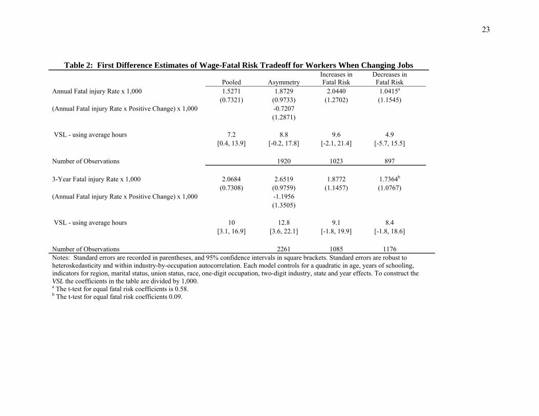
Table 2: First Difference Estimates of Wage-Fatal Risk Tradeoff for Workers When Changing Jobs





(1.2871)

VSL - using average hours 7.2 8.8 9.6 4.9 [0.4, 13.9] [-0.2, 17.8] [-2.1, 21.4] [-5.7, 15.5]

Number of Observations 1920 1023 897



(1.3505)

VSL - using average hours 10 12.8 9.1 8.4 [3.1, 16.9] [3.6, 22.1] [-1.8, 19.9] [-1.8, 18.6]

Number of Observations 2261 1085 1176 Notes: Standard errors are recorded in parentheses, and 95% confidence intervals in square brackets. Standard errors are robust to heteroskedasticity and within industry-by-occupation autocorrelation. Each model controls for a quadratic in age, years of schooling, indicators for region, marital status, union status, race, one-digit occupation, two-digit industry, state and year effects. To construct the VSL the coefficients in the table are divided by 1,000. a The t-test for equal fatal risk coefficients is 0.58. b The t-test for equal fatal risk coefficients 0.09.

24

Table 3: Selection-Corrected Estimates of Wage-Fatal Risk Tradeoff for Workers Ever Changing Jobs





(1.2054)





(1.2497)

VSL - using average hours 12.3 13.6 16.3 8.0 [4.4, 20.2] [4.6, 22.7] [3.8, 28.9] [-3.2, 19.2]

Number of Observations 3315 3315 1488 1827 Notes: Standard errors are recorded in parentheses, and 95% confidence intervals in square brackets. Standard errors are robust to heteroskedasticity and within industry-by-occupation autocorrelation. Each model controls for a quadratic in age, years of schooling, indicators for region, marital status, union status, race, one-digit occupation, two-digit industry, state and year effects. To construct the VSL the coefficients in the table are divided by 1,000. a The t-test for equal fatal risk coefficients is 0.49. b The t-test for equal fatal risk coefficients 1.02.

25

Table 4: Difference-in-Difference Estimates of Wage-Fatal Risk Tradeoff for Workers Ever Changing Jobs




(0.6677) (0.8257) (1.0452) (1.0127) (Annual Fatal injury Rate x Positive Change) x 1,000 0.0938

(1.1271)





(1.2095)

VSL - using average hours 12.1 13.1 7.1 12.7 [4.6, 19.5] [3.5, 22.6] [-3.8, 18.1] [1.9, 23.5]

Number of Observations 2273 2273 1195 1078 Notes: Standard errors are recorded in parentheses, and 95% confidence intervals in square brackets. Standard errors are robust to heteroskedasticity and within industry-by-occupation autocorrelation. Each model controls for a quadratic in age, years of schooling, indicators for region, marital status, union status, race, one-digit occupation, two-digit industry, state and year effects. To construct the VSL the coefficients in the table are divided by 1,000. a The t-test for equal fatal risk coefficients is -0.06. b The t-test for equal fatal risk coefficients -0.74.

26

Table 5: Difference-in-Difference Estimates of Wage-Fatal Risk Tradeoff for Workers When Changing Jobs




(0.7125) (0.8575) (1.1493) (1.0704) (Annual Fatal injury Rate x Positive Change) x 1,000 0.2843

(1.2233)





(1.3047)

VSL - using average hours 12.5 13.4 7.2 13.1 [4.8, 20.3] [3.4, 23.4] [-1.8, 19.9] [1.7, 24.5]

Number of Observations 1898 1898 985 913 Notes: Standard errors are recorded in parentheses, and 95% confidence intervals in square brackets. Standard errors are robust to heteroskedasticity and within industry-by-occupation autocorrelation. Each model controls for a quadratic in age, years of schooling, indicators for region, marital status, union status, race, one-digit occupation, two-digit industry, state and year effects. To construct the VSL the coefficients in the table are divided by 1,000. a The t-test for equal fatal risk coefficients is 0.14. b The t-test for equal fatal risk coefficients -0.75.

27

Appendix A: Variable Means for Alternative Samples Used in

Estimation

Ever Change Industry / Occupation

When Change Industry / Occupation

Real Hourly Wage 20.80 20.70 Log Real Hourly Wage 2.89 2.87 Annual Hours of Work 2281.94 2269.27 Age 41.05 40.84 Marital Status (1=Married) 0.82 0.81 Race (1=White) 0.78 0.78 Union (1=member) 0.19 0.17 Years of Schooling 13.40 13.36 Live in Northeast 0.18 0.18 Live in Northcentral 0.30 0.30 Live in South 0.37 0.37 Live in West 0.15 0.15

One-Digit Industry Groups: Mining 0.01 0.01 Construction 0.12 0.12 Manufacturing 0.28 0.29 Transportation and Public Utilities 0.13 0.11 Wholesale and Retail Trade 0.14 0.15 Fire, Insurance, and Real Estate 0.04 0.04 Business and Repair Services 0.09 0.10 Personal Services 0.01 0.01 Entertainment and Professional Services 0.15 0.13 Public Administration 0.05 0.05

One-Digit Occupation Groups: Executive and Managerial 0.22 0.23 Professional 0.13 0.12 Technicians 0.05 0.05 Sales 0.03 0.03 Administrative Support 0.04 0.04 Services 0.07 0.06 Precision Production Crafts 0.24 0.24 Machine Operators 0.08 0.09 Transportation 0.09 0.08 Handlers and Labors 0.05 0.06

Annual Fatal injury Rate (per 100,000) 6.31 6.21 3-Year Fatal injury Rate (per 100,000) 6.15 6.03

Number of Person Years 3035 1920 Note: Samples are for person years where the change in the annual fatal injury rate is greater than -80%

and less than 300%. Subcategories may not sum to 1 due to rounding.

Date post:	22-Apr-2018
Category:	Documents
Upload:	dinhnga
View:	222 times
Download:	1 times

Willingness to Accept Equals Willingness to Pay for …ftp.iza.org/dp6816.pdfA revised version may...

Documents