The parallels between wind excited structures and wind excited musical instruments are the basic idea of this paper. Vibrations of structures are caused by the same self-excited or motion-induced me-chanisms as the vibration in musical instruments. Vibrating engineering structures just produce music at inaudible frequencies. The paper deals with both parts: on the one hand with waves or high frequency vibrations, i.e. sound and music, and on the other hand with low-frequency vibrations of civil structures like towers, masts, bridges etc. Because many of the sound generating mechanisms show a feedback with the instrument itself, some basics of wave propagation and dynamics of musical instruments are dis-cussed first. Concerning the wind engineering topic, latest research results of the wind engineering group at the Institute for Steel Structures at the Technische Universität Braunschweig, Germany are briefly presented.
1 To Carola Bethge, Wolfenbüttel who has aroused my interest for this fascinating topic.
Wind effects are often responsible for severe vibration of structures but on the other hand they also may cause music. Resounding thin wires in the natural wind are well known examples. Aeolian harps (see Fig. 1) have been used for thousands of years. In such a harp one or more prestressed wires are excited due to vortex excitation by the streaming air, the sound is amplified by a resonance body. The equation of the vortex frequency is well known to wind engineers:
0.2 [ ]v
f Hzd
= (1)
with v as wind speed in [m/s] and d as diameter of the string in [m]. A wind speed of 5m/s causes a tone of 1000Hz with a 1-mm thick string. If the string is tuned to this frequency, a mysterious, me-lancholic and vague sound is produced.
Two types of sound generation mechanisms occur: first the direct vortex-induced sound and in addition the higher harmonics, the so called overtones of the string itself. Depending on the wind speed, the pitch often changes. This basic excitation effect is also well known in wind engineering: It generates music or structural vibrations, which could be interpreted as music at inaudible frequencies.
In this paper the tone or sound generating mechanisms of wind instruments are discussed and compared with wind excitation processes in wind engineering. Because many of the sound generating mechanisms show a feedback with the instrument itself (just as structural wind excitations often do) some basics of wave propagation and dynamics of musical instruments are discussed first. Con-cerning the wind engineering field, latest research results of my wind engineering group at the at the Institute for Steel Structures at the Technische Universität Braunschweig, Germany are briefly pre-sented.
2. WAVES AND VIBRATIONS
A wave is a disturbance that propagates through space and time, usually combined with a transfer of energy, which is not associated with a motion of the medium. It oscillates somewhat around its me-dium position. Mechanical waves may take the form of an elastic deformation or of a variation of pressure.
If two waves with the same amplitude, frequency, and wavelength, but varying phase difference travel in the same direction, the resulting displacement is given in equation 2. The resulting wave is a
Figure 1: Aeolian harp
travelling wave whose amplitude depends on the phase φ. When the two waves are in phase (φ=0°) they add up, i.e. they interfere constructively and the result has twice the amplitude of the individual waves. When the two waves have opposite phase (φ=180°), they interfere destructively and cancel out each other:
( , ) sin ( ) sin ( )
2 cos sin2 2
A m
A
y x t y kx t y kx t
y kx t
ω ω φ
φ φω
= ⋅ − + ⋅ − +
= ⋅ ⋅ ⋅ − +
(2)
If two waves with the same amplitude, frequency, and wavelength travel in opposite direction, they cause a so called standing wave. Using the principle of superposition, the resulting string displace-ment can be written as:
( , ) sin( ) sin( )
2 sin cos
A m
A
y x t y kx t y kx t
y kx t
ω ω
ω
= ⋅ − + ⋅ +
= ⋅ ⋅ ⋅ (3)
At any change of the mechanical properties of the wave guiding medium or at the boundary condi-tions, the wave is fully or partly reflected. The reflection is dependent on the type of the boundary condition. A rope or a string, which is fixed at its ends, reflects a wave by changing its sign. A wave in a tube (as a simple model for a pipe or another wind instrument) is reflected at the end of the tube, may it be open or closed. If the end of the tube is open, then the last element at the opening which is pushed by the penultimate element does not have a neighbor element to which the impact can be transferred, the mass inertia is missing. Therefore it moves out, but it is kept by the low pressure which pulls it back into the tube. The pressure sign changes, oncoming pressure is reflected as low pressure and vice versa, cf. Fig. 2. If the pipe is closed, the last element can’t move, thus it gets the maximum pressure and gives it back to the penultimate element without changing its sign: oncoming pressure remains pressure and low pressure remains low pressure after reflection at a closed end, see Fig. 3. The reflected wave then travels back through the tube and interferes with the oncoming wave. If a pipe is harmonically excited at one end, both above mentioned principles interfere. If the fre-quency of the excitation is such that the generated half wave length fits into the pipe’s length, then the reflected wave is perfectly pushed in phase, a large standing wave is generated due to the constructive interference, the excitation is a resonant one. If the frequency of excitation is slightly changed, then the excited wave does not exactly fit the phase of the reflected one, destructive interference occurs, the resulting standing waves show reduced amplitudes, it is a non-resonant excitation. If the excita-tion frequency is further changed then suddenly a new standing wave occurs with one more half wave length. When the frequency is increased further, a new standing wave with an additional half wave and an accompanying resonant peak occurs, see Fig. 3.
Figure 2: Reflections
Figure 4: Transverse and longitudinal vibration
The standing wave generated by the travelling and reflected waves may be interpreted as a usual vibration. The behavior of a vibrating system (string, pipe, bridge) can be explained by wave su-perposition or by vibration theory. It is the same from two different points of view.
3. NATURAL FREQUENCIES OF STRINGS AND PIPES
Since a simple vibrating string is much easier to imagine than a non-visible longitudinal air vibration in a flute, a clarinet, an oboe or trumpet, some basics are explained first, using the string. Fortunately a transversely vibrating string and the longitudinally vibrating air in a flute or another wind instru-ment are differ only concerning the direction of vibration, see Fig.4.
The natural frequency of a vibrating string is known to be
1 1[ ]
2
Sf Hz
l m= ⋅ (4)
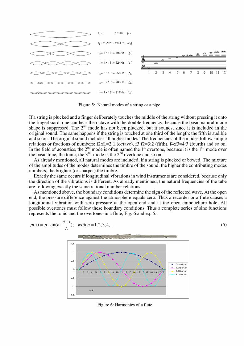
l is the length, S the pretension force and m the mass of the string. To tune the pitch of the string, the pretension force of the string is adjusted by the peg of the violin. The frequency is then directly de-pendent on the length of the string: half the length means twice the frequency and so on. The ac-companying natural modes are sine waves. The wave length of the n-harmonic has a length of l/n, see Fig. 5. Thus the 2
nd mode has a natural frequency which is twice the basic one (octave), the 3
rd natural
frequency has three times the basic frequency etc. The accompanying notes are shown in Fig. 5.
If a string is plucked and a finger deliberately touches the middle of the string without pressing it onto the fingerboard, one can hear the octave with the double frequency, because the basic natural mode shape is suppressed. The 2
nd mode has not been plucked, but it sounds, since it is included in the
original sound. The same happens if the string is touched at one third of the length: the fifth is audible and so on. The original sound includes all higher modes! The frequencies of the modes follow simple relations or fractions of numbers: f2:f1=2:1 (octave), f3:f2=3:2 (fifth), f4:f3=4:3 (fourth) and so on. In the field of acoustics, the 2
nd mode is often named the 1
st overtone, because it is the 1
st mode over
the basic tone, the tonic, the 3rd
mode is the 2nd
overtone and so on. As already mentioned, all natural modes are included, if a string is plucked or bowed. The mixture
of the amplitudes of the modes determines the timbre of the sound: the higher the contributing modes numbers, the brighter (or sharper) the timbre.
Exactly the same occurs if longitudinal vibrations in wind instruments are considered, because only the direction of the vibrations is different. As already mentioned, the natural frequencies of the tube are following exactly the same rational number relations.
As mentioned above, the boundary conditions determine the sign of the reflected wave. At the open end, the pressure difference against the atmosphere equals zero. Thus a recorder or a flute causes a longitudinal vibration with zero pressure at the open end and at the open embouchure hole. All possible overtones must follow these boundary conditions. Thus a complete series of sine functions represents the tonic and the overtones in a flute, Fig. 6 and eq. 5.
( ) sin( ); 1,2,3,4,...x
p x p n with nL
π ⋅= ⋅ ⋅ = (5)
f5 = 5 • 131= 655Hz (e2)
f6 = 6 • 131= 786Hz (g2)
f7 = 7 • 131= 917Hz (b2)
f1 = 131Hz (c)
f2 = 2 •131 = 262Hz (c1)
f3 = 3 • 131= 393Hz (g1)
f4 = 4 • 131= 524Hz (c2)
Figure 5: Natural modes of a string or a pipe
Figure 6: Harmonics of a flute
All other wind instruments have a mouthpiece, which seals the internal pressure against the outside atmosphere. The mouthpiece closes the pipe, thus the wave is reflected without changing its sign. Therefore the pressure reaches its maximum at the mouthpiece. The pressure distribution along a cylindrical pipe can be represented by half sine functions, with a maximum at the mouthpiece and zero pressure at the open end, see Fig. 7. Thus a series of sine functions consisting only of the odd numbers occurs:
( ) sin( ); 1,3,5,7,...2
xp x p n with n
L
π ⋅= ⋅ ⋅ =
⋅ (6)
This is typical of a clarinet. Especially the missing 1st overtone leads to the dark and a little bit hollow
sound. The wavelength of the sine functions of a cylindrical pipe with a mouthpiece is twice the wave length of the flute. Therefore the pitch of the tone is one octave below a flute. This effect is often used for organ pipes. If the open end of a pipe is closed, the pipe sounds one octave lower. This method is much cheaper than to build pipes with twice the length.
If pressure and air speed is increased, the instrument overblows, the pipe jumps into the second mode and the 1
st overtone sounds. A flute therefore plays an octave higher. A clarinet overblows in its
1st overtone as well, but it is one fifth higher than the flute, it is the twelfth (octave + fifth) because the
even mode is missing. The overblowing effect can be supported by opening a matching finger hole. If for instance a flute opens the c-key, which is exactly in the middle between the mouthhole (embou-chure hole) and the open end, than the basic sine wave is suppressed, because the open hole forces the pressure at its maximum to zero, the 2
nd harmonic or the 1
st overtone becomes now the tonic.
Just a surprising effect shall be discussed at the end of this section. As has been mentioned above, all reed instruments have the boundary condition of a closed tube at the mouthpiece because the lips seal the internal pressure against the free atmospheric pressure. Therefore all reed instruments should overblow into the twelfth as explained above. But only the clarinet performs as expected. What is the reason for this deviating behavior from all other reed instruments?
The reason is the shape of the bore. Only the clarinet has a cylindrical bore, which is what was assumed above in all explanations. All other reed instruments like oboe, bassoon and saxophone have a conical bore. Fig. 8 shows a longitudinal section of clarinet and an oboe. The cylindrical and conical shape is clearly visible. The conical bore considerably changes the acoustic behavior.
The sound in a conical tube changes its intensity and pressure as a function of the distance from the sound generator, the mouthpiece. If we measure the pressure at the open end and then step by step towards the mouthpiece we find that the pressure increases linearly depending on the decreasing distance from the mouthpiece. The approximately constant sound pressure must pass the tapering bore, with a continuously decreasing area, if we look from the open end to the mouthpiece, Fig. 9.
Figure 7: Harmonics of a closed cylindrical pipe (clarinet for instance)
This linearly increasing pressure can be taken into account by an amplitude factor 1/r of the sine wave:
1( ) sin( ); 1,3,5,7,...
2
xp x p n with n
r L
π ⋅≈ ⋅ ⋅ ⋅ =
⋅ (7)
The known odd numbers of the sine waves fulfill the boundary conditions at the closed end: the pressure has a maximum, Fig. 12 left. An even sine wave however does not fulfill this boundary condition (Fig. 10 right). But due to the additional factor 1/r, the pressure p(r) increases near the bore, so the pressure boundary condition can be met, Fig. 12 right. The wave length of the amplitude modified sine wave is the wave length of the original sine wave, with the even wave number. Thus all harmonics, i.e. all overtones, are sounding and the conical bored instruments overblow into the 1
st
overtone, i.e. into the octave.
Due to the standing waves, the pressure at the embouchure hole changes harmonically from over-pressure to low pressure. This harmonically alternating pressure drives the excitation mechanism of all wind instruments fro m flutes to reed and to brass instruments.
Figure 8: Bore of a clarinet and an oboe
Figure 9: Sound pressure reduction with increasing distance from the mouth piece
-1,5
-1
-0,5
0
0,5
1
1,5
1 3 5 7 9 11 13 15 17 19 21
Grundton
1.Oberton
-1,5
-1
-0,5
0
0,5
1
1,5
1 3 5 7 9 11 13 15 17 19 21
1/r * sin
sin
Figure 10: Influence of a conical bore on the action of even harmonics
4. NATURAL MODES AND OUR MUSIC SCALE
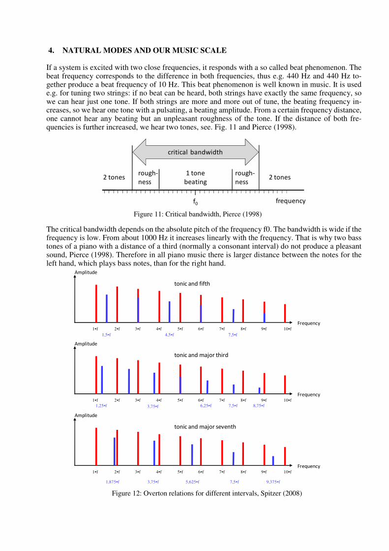
If a system is excited with two close frequencies, it responds with a so called beat phenomenon. The beat frequency corresponds to the difference in both frequencies, thus e.g. 440 Hz and 440 Hz to-gether produce a beat frequency of 10 Hz. This beat phenomenon is well known in music. It is used e.g. for tuning two strings: if no beat can be heard, both strings have exactly the same frequency, so we can hear just one tone. If both strings are more and more out of tune, the beating frequency in-creases, so we hear one tone with a pulsating, a beating amplitude. From a certain frequency distance, one cannot hear any beating but an unpleasant roughness of the tone. If the distance of both fre-quencies is further increased, we hear two tones, see. Fig. 11 and Pierce (1998). The critical bandwidth depends on the absolute pitch of the frequency f0. The bandwidth is wide if the frequency is low. From about 1000 Hz it increases linearly with the frequency. That is why two bass tones of a piano with a distance of a third (normally a consonant interval) do not produce a pleasant sound, Pierce (1998). Therefore in all piano music there is larger distance between the notes for the left hand, which plays bass notes, than for the right hand.
Figure 12: Overton relations for different intervals, Spitzer (2008)
1•f 2•f 3•f 4•f 5•f 6•f 7•f 8•f 9•f 10•f
1,5•f 7,5•f4,5•f
Amplitude
Frequency
tonic and fifth
1•f 2•f 3•f 4•f 5•f 6•f 7•f 8•f 9•f 10•f
Amplitude
Frequency
tonic and major third
1•f 2•f 3•f 4•f 5•f 6•f 7•f 8•f 9•f 10•f
1,875•f 5,625•f3,75•f 7,5•f 9,375•f
Amplitude
Frequency
tonic and major seventh
1,25•f 6,25•f3,75•f 7,5•f 8,75•f
Figure 11: Critical bandwidth, Pierce (1998)
1 tone
beating
rough-
ness
rough-
ness2 tones2 tones
critical bandwidth
f0 frequency
Figure 13: Discrepancy of intervals
12
11
10
9
8
7
6
5
4
3
2
1
h#7
e#7
a#6
d#6
g#5
c#5
f#4
h3
e3
a2
d2
g1
c1
c8
c7
c6
c5
c4
c3
c2
c1
12
7
3# 131 16996
2h Hz Hz
= ⋅ =
7
8 7
2# 131 16768
1c h Hz Hz
= = ⋅ =
By the way: The simple number relations between the basic tone (tonic) and the overtones are re-sponsible for our usual diatonic scale system. If this scale is used for polyphonic music then many overtones are identical. The sound is harmonic or consonant, only few overtones are inharmonious. This is shown in Fig. 12. The tonic and the fifth have many identical overtones. Some overtones are in between, but the distance is large, no beat phenomena occur. The tonic and the major third are a little bit rougher, in earlier times this interval was considered to be dissonant. The tonic and the major seventh have no identical overtones. The overtones are very close and therefore produce beating phenomena, the sound is dissonant, it “whimpers”, Spitzer (2008).
Only strings and wind instruments with a tube as resonator show the above mentioned simple number relations of overtones which can be expressed by fractions. A bell for instance has a 1
st
overtone of about 2.3•f, the 2nd
is about 3.5•f and the 3rd
is 4.8•f. This overtone spectrum does not fit for different basic tones (tonics). Thus polyphonic bell music is not very pleasing to the ears, too many overtone dissonances occur.
As already mentioned, our usual music scale is based on the natural modes of a string. All intervals result from the relations over the overtones. As mentioned above, a fifth has always a frequency re-lation to the tone it is related to of 3/2=1.5, an octave has the relation 2/1=2, a major third 5/4 and so on. This leads to serious problems with the music scale. If we staple 12 fifth, starting for instance with a c1 with a frequency of 131Hz, the fifth is 1.5•131Hz (g1). The next fifth to this note is 1.5•1.5•131Hz and so on. The 12
th fifth is the h#7, it has a frequency of 16996 Hz, see Fig. 13. The note h#7 cor-
responds to the c8 key of the piano, see Fig. 13. This tone can also be reached by 7 octaves. The next octave to c1 is 131 •2 Hz (c2). Stapling 12 octaves in this way we reach c8 with 16768Hz, which differs by 1.36% from the same note generated by the fifths, see Fig. 13
This is a serious problem which occupied many people in the past, starting with Pythagoras who found this problem about 550 BC. Many different tuning systems have been developed to overcome this problem: well tempered, mean tone, equal temperament, Werckmeister temperament etc.
5. EXCITATION MECHANISMS
5.1 Sound excitation
The simplest sound producing excitation mechanism is whistling. How is the sound generated? When air is forced through a small opening or slit e.g. the narrow opening formed by the lips, the fast air-stream moves through slower air. The boundaries of the airstream get resistance from that slower air and tend to peel back and form vortices. These vortices interact with the stream, causing it to move in an undulating path, Fig. 14.
This undulation can actually produce a substantial amount of sound. The undulations in the stream move along the stream at something less than one half the speed of the air in the stream, Hall (1991). The faster the airstream speed, the faster the oscillations of the stream. In addition, the oscillating stream causes a feedback to the lips and the oral cavity (acting as a Helmholtz resonator) thus the pitch can be influenced by both.
An even greater amount of sound can be produced by coupling the slit to an edge. The airstream is separated by a sharp edge and a type of repetitive eddying called vortex shedding takes place on al-ternate sides of the air jet, like a vibrating air tongue or air reed, see Fig. 15, Hall (1991). Vortex phenomena have only a secondary influence on flute-type sound production; moreover, at usual musical blowing pressures the edge-tone frequencies are so high as to be nearly inaudible. They are only used to initiate the vibration. The impulse produced by the edge tone causes a travelling wave in the bore of the flute. This wave is reflected at the open end and then forms a standing wave with alternating harmonic pressure variation at the nearly open mouthpiece with the edge or labium. The alternating pressure now takes control over the movement of the air reed. The alternating pressure of the standing wave causes self-excited vibration of the air reed of the flute, see Fig. 16. If the alternating pressure of the standing wave at the labium is lower than the atmospheric pressure, then the air reed is sucked into the pipe; if the pressure is higher than it is pushed out. Thus the vibrating system is excited exactly in resonance of the pipe.
Fig. 17 is a snapshot of the fluctuating pressure in the bore of the flute. It is calculated by means of the CFD-method using the Lattice-Bolzmann procedure, Tölke et al. (2008). The calculation was performed by the group of Prof. Manfred Krafczyk at the Technische Universität Braunschweig. One can see the alternating pressure distribution, and the vortexes near the labium.
Figure 14: Basic mechanism of whistling
Lip slit
~0.4 •v
v
Figure 15: Edge tone excitation
d
0.2 vf
d
⋅=
v
Fig. 18 shows the calculated amplitude spectrum of the simulation at the open end of the flute. The overtones are reproduced quite well, the basic frequency (tonic) is correct.
The above mentioned excitation mechanisms of the oscillating air stream around an edge can be di-rectly used as an explanation for all reed or brass instruments. Fig. 19 shows mouthpieces of a clarinet with a single reed and an oboe with a double reed.
Figure 17: Fluid pressure distribution in an alto recorder
suction
compression
compression
suction
Figure 16: Schematic feedback mechanism for the synchronization of the air reed
Figure 19: Mouthpieces of a clarinet and an oboe
Figure 18: Amplitude spectra at the open end of the recorder
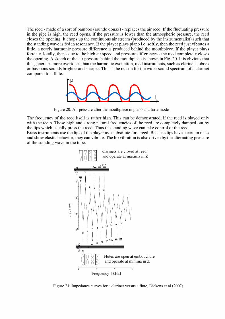
The reed - made of a sort of bamboo (arundo donax) - replaces the air reed. If the fluctuating pressure in the pipe is high, the reed opens, if the pressure is lower than the atmospheric pressure, the reed closes the opening. It chops up the continuous air stream (produced by the instrumentalist) such that the standing wave is fed in resonance. If the player plays piano i.e. softly, then the reed just vibrates a little, a nearly harmonic pressure difference is produced behind the mouthpiece. If the player plays forte i.e. loudly, then - due to the high air speed and pressure differences - the reed completely closes the opening. A sketch of the air pressure behind the mouthpiece is shown in Fig. 20. It is obvious that this generates more overtones than the harmonic excitation, reed instruments, such as clarinets, oboes or bassoons sounds brighter and sharper. This is the reason for the wider sound spectrum of a clarinet compared to a flute. The frequency of the reed itself is rather high. This can be demonstrated, if the reed is played only with the teeth. These high and strong natural frequencies of the reed are completely damped out by the lips which usually press the reed. Thus the standing wave can take control of the reed. Brass instruments use the lips of the player as a substitute for a reed. Because lips have a certain mass and show elastic behavior, they can vibrate. The lip vibration is also driven by the alternating pressure of the standing wave in the tube.
Figure 20: Air pressure after the mouthpiece in piano and forte mode
p
t
Figure 21: Impedance curves for a clarinet versus a flute, Dickens et al (2007)
Frequency [kHz]
Flutes are open at embouchure
and operate at minima in Z
clarinets are closed at reed
and operate at maxima in Z
The behavior of a flute and a clarinet as an example of a pipe, that is open at both ends and a pipe that is open at one and closed at the other end, can be quantified, both theoretically and experimentally, using the acoustic impedance spectrum. It is defined as the ratio of the acoustic (varying) pressure required at the system input (mouthpiece or embouchure) to produce the acoustic flow in the tube. Its dimension is N/m² s m-3. In an infinite pipe, a harmonically varying pressure causes a wave which never comes back. In a finite pipe, however, the wave reflects at the far end and causes standing waves (resonance), which alters the impedance remarkably. In Fig. 21 the impedance curve of a pipe closed at one end and open at the other and a pipe open at both ends is shown, Dickens et al (2007).
One can see that the clarinet operates at maxima and the flute in minima of the impedance. A reed of a clarinet needs relatively high pressure to move from its initial position; the air reed of a flute operates at small pressure otherwise it would be blown away. Operating at maxima of impedance means that the acoustic swing is pushed when the pressure is high and the speed is very slow. This is the upper point of a swing, i.e. the maximum potential energy. On the other hand operating at minima of impedance means that the pressure is low but the flow is high. The flute pushes the swing at the lowest point, when the speed is high, but the potential energy has a minimum. The ease of playing and the stability of a note depend on the peak and narrowness of the maxima or minima. The impedance curve in Fig. 21 is measured with a closed-open pipe. If measurements are per-formed with a real clarinet, then the harmonics deviate from maxima of the impedance curve. This is due to the bell, which gives the instrument an effective length that increases with frequency. Fur-thermore the amplitudes of the extremes are reduced with increasing frequency due to the bell: The bell radiates especially high frequencies, thus the reflected part of the wave is smaller and the wave is weaker.
Another interesting point is the behavior of the tone holes. As already mentioned, the tone holes open the bore to the outside atmospheric pressure, thus it shortens the effective length of the tube. This is only true for low frequencies: the wave is reflected at (or near) this open tone hole because the hole provides a low impedance with low resistance to the outside air. For high frequencies, however, that does not hold true. The air in and near the tone hole provides some mass. This mass has to be accelerated by the sound wave when it passes through the tone hole. The required acceleration to move the mass increases with the square of the frequency: for a high frequency wave there is little time in half a cycle to get it moving, see Fig. 22. The tone hole acts like a low pass filter: the low frequencies leave through the holes, the high ones through the bell. This effect is used for instance by Gustav Mahler: In his symphonies, special the clarinet group has to lift the instruments sometimes in a horizontal position. The acoustic effect is such that the radiated sound becomes brighter and may be sharper due to the better transferred high frequencies.
Due to the inertia of the air mass in the tone holes, the pressure is always a little bit higher than the outside atmospheric pressure. Thus the effective length is always a little bit longer than the tone hole pretends.
waves with low frequencies are
radiated and reflected at the hole
waves with high frequencies are
travelling through
air mass in open tone holes
from
mouth piece
Figure 22: Behavior of tone holes as low pass filters
Figure 23: Typical wind profile classes at lower wind speed (ο: u �: Iu)
5.2 Structural vibration excitation
The vibration excitation mechanisms of structures in natural wind are identical to those exciting musical instruments. The already mentioned aeolian harp is an example of vortex induced vibrations of slender structures like chimneys or masts. The string of the wind harp is excited by a wind field which may be assumed to be constant over the small length of the structure (the string). This as-sumption is also generally used in wind engineering. Since the critical wind speed, which causes resonant lateral vibrations in the structure, is only low but normally shows extremely varying profiles, the assumption of a constant profile is an easy way out but not a realistic one. Fig. 24 shows some profiles measured at our wind measuring mast at Gartow, Germany together with approximations.
First the measured wind profiles are classified in predefined classes which are assessed looking over a wide range of measurements, Fig. 25 shows the principle. Every single class can then be described by a vector µ of the mean wind speed and the covariance matrix cov. In a second step, the profiles will be assigned to typical wind climate situations, thus the duration time can be determined using synoptic weather data. This is important for assessment of the fatigue life time of the structure.
Figure 24: Statistical classification of wind profiles
profiles of class A
wind speed U
measurement
pattern classall measured profilesof the class
probability density
correlation coefficient
he
igh
t z
The determination of structural response due to vortex vibration is a complex problem, because the relation between wind force and speed is quadratic. In addition, the transfer matrix H (iωn) is coupled with the random variable U via the excitation frequency and the Strouhal number. Thus the calcula-tion is performed using the Monte Carlo Method together with variance reducing methods like lat-in-hypercube or importance sampling, see Fig. 26. The lock-in effect can be taken into account by an iteratively adapted excitation frequency. Fig 26 shows as an example the influence of the lock-in process at a 205-m high guyed mast with a circular shaft. The deflections of the mast top are shown. The occasionally occurring vibrations up to approximately the half of the maxima, is caused by resonance excitation at lower heights. When starting at t=350s the excitation frequency at the mast top is in the lock-in range. This causes imme-diately a strong increase of the lateral vibrations. After t=420s, the excitation frequency leaves the lock-in range, the lateral vibration are reduced straight. The longitudinal vibrations are stochastic as expected. More details are given in Clobes et al. (2009).
The second above mentioned sound excitation mechanism is a self-excited or motion-induced feedback process of the reed, which is controlled by the pressure variation of the standing wave. This is a process very close to flutter excitation, e.g. of long span bridges. What are we doing in this field?
Flutter vibrations of bridge girders can result in the collapse of the structure within a short time. The Tacoma Narrows Bridge disaster is a well-known example of bridge flutter. Flutter vibrations are generated by so-called motion-induced aerodynamic forces. Together with its structural parameters,
Figure 25: Description of vortex excitation as a probabilistic, correlated harmonic forced vibration
time t [s]
Figure 26: Time history of excitation frequency and corresponded deflection of the mast top
motion-induced wind forces influence the properties of an aeroelastic system. To provide against these phenomena, two standard methods are used to ensure the stability of an aeroelastic bridge system: either the bridge girder is designed with a high torsional stiffness or the girder cross section is aerodynamically optimised.
In recent years, inspired for instance by aerospace engineering, a number of techniques have been investigated to improve the vibration behaviour of extremely slender bridges under wind action with systematically imposed forces. Fig. 27 shows three kinds of actuators that have been proposed for this purpose in the past. Inertial forces can be generated when accelerating a reaction wheel (Miyata et al. 1994; Körlin & Starossek 2007). Rotating gyroscopes that are mounted in a tiltable gimbal can affect the bridge with gyroscopic forces (Murata & Ito 1971). The motion of the actuators can be controlled in different ways. Active and passive controllers are the most important types of control-lers. An example of a passive controller is the coupling of the actuator motion with the bridge girder by spring-damper systems. Passive controllers are normally low-maintenance devices and need no energy input. In the case of gyroscopes, only their spin must be kept constant. Passive controllers can be considered as an output feedback that, moreover, has sign constraints for the controller values. With methods of control theory, it can easily be shown that their effectiveness is limited. The cha-racteristics of an aeroelastic system depend on the mean horizontal wind speed. Passive controllers cannot be easily adjusted to these changing conditions. For a wide range of the horizontal mean wind speed, the properties of passive controllers are not optimised. Active controllers, on the other hand, can induce energy into the bridge girder and, if configured appropriately, can take the total state of the aeroelastic system into account. The properties of active controllers can be adjusted to the horizontal mean wind speed without problems. Compared to passive ones, active controllers can thus stabilize the bridge within a wider speed range. This feature, however, causes serious safety problems in permanent operation. Anyway, at least for construction stages of bridges with undesirable aeroelastic characteristics, active controllers are considered to be a useful option. In Peil & Kirch (2008), control limits for slender bridges under wind action are investigated. It is shown that the divergence wind speed of the bridge constitutes an upper limit for the application of the mentioned mechanical actu-ators.
Fig. 27 additionally shows aerodynamically effective control shields as a kind of actuator that was proposed several years ago for extremely slender bridges (Kobayashi & Nagaoka 1992; Ostenfeld & Larsen 1992). In contrast to the other mentioned actuators, the divergence wind speed of the system can be modified as well. The crucial advantage of aerodynamically effective control shields is that additionally imposed forces on the bride deck are generated by the wind flow. Aerodynamically ef-fective, movable control surfaces have been used in aerospace engineering to suppress the influences
Figure 27: Actuators for stabilising bridges under wind action: aerodynamically effective control shields,
twin control moment gyroscope and reaction wheel.
Figure 28: Ice accretion on single cables with different diameter
of disturbances on aircraft wings for many years. With bridges, however, control shields are extra components that augment the area exposed to the wind. They cannot bear any significant payload and can hence not directly fulfil the intrinsic task of a bridge. In addition to motion-induced aerodynamic forces, new gust-induced forces arise simultaneously, which also need to be suppressed. Therefore, aerodynamically effective control shields are generally less effective for bridges than for aircraft wings. Moreover, control shields need a minimum wind speed to work. They are not suited for damping oscillations in still air. The motion of the control shields can again be controlled actively and passively. Fundamental control limits for bridges equipped with aerodynamically effective control shields are investigated in Kirch & Peil (2009a/b).
A related topic to flutter is galloping as another type of motion-induced vibrations. In particular iced cables often show this type of vibration with low frequencies and large vibrations. Iced cables have a shape which is aerodynamically instable, i.e. when the wind speed reaches a certain value, galloping vibrations occur, because the structure velocity dependent air pressure equals the velocity dependent damping of the structure; the overall damping is zero or becomes negative if the wind speed further increases.
The theoretical treatment is fairly simple. Determining ice shapes dependening on wind and snow or rain characteristics is rather difficult. Ice accretion on conductor bundles can be investigated with experiments or with statistical and numerical models. Experiments are difficult to perform.
In theoretical investigations, both shape and aerodynamic coefficients require simulation of the icing process itself. Known numerical models are restricted to single cables due to the assumptions made in the flow calculation. With the simulation scheme used at our institute, the particle motion based on the stream around the conductor bundles can be determined. The simulation uses a Finite Element Method (FEM) with a Reynolds Average Navier-Stokes (RANS) for an incompressible fluid via a k-ε turbulence model. The stream of air and of precipitation droplets are modelled as one-way coupled two-phase flow. Ice accretion and flow field are calculated iteratively to account for geometrical changes of the ice deposit in the flow calculation. Modelling atmospheric icing includes, in addition, a computation of the mass flux of icing particles as well as a determination of the icing conditions: Icing conditions are defined by the heat balance on the ice surface, Peil & Wagner (2008) and Wagner, Peil & Borri (2009).
Three major types of deposit, namely rime, glaze and wet snow lead to significant loads on structures. For glaze ice and wet snow formation, the heat balance on the ice surface is very important. Computation of the mass flux of icing particles is an important factor in ice accretion. Shape, and to a smaller extent, also density of ice evolution is influenced by the characteristics of the particle trajectories.
Figure 28 shows, on the left, results of simulations with the presented model (−), with the model of Fu (2006) (· · ·) and with eperiments (- -).The presented model meets the longitudinal extension of the ice body very well for a larger (left) and a smaller (right) cable diameter. The vertical extension deviates in both cases, which is due to the calculation of the particle impinging points on the surface.
Fig. 29 shows the simulation of ice accretion on a bundle of two cables. The upstream cable catches a larger fraction of the particle flux than the downstream cable in its wake. In general, the shaded area decreases with decreasing deflection of the particle trajectories. It means that larger droplets will deflect less due to their higher inertia. Once the upstream cable gets a more streamlined shape due to the ice accretion, the particle trajectories are deflected to a smaller extent when passing the first cable. Thus the mass flux on the downstream cable increases.
An also motion-induced or self-excited excitation mechanism is the so called rain-wind induced vi-bration. They are very close to galloping vibrations, except that the shape of the vibrating (iced) cable is not constant over time but varies due to the fluctuating rivulets produced by rain, wind and inertia. In contrast to galloping vibrations, there is not only an onset wind speed, but also a final wind speed beyond the vibration ends. The onset wind speed is not high, about 5m/s could be enough. The final wind speed could be about 15 to 20m/s. The vibration is mainly controlled by damping. The stability plot in Fig. 30 shows that even small damping decrements abandon the vibration, Peil, Narath & Dreyer (2003). A state-of-the- art report is published in Peil & Steiln (2007).
The investigations are performed under the assumption of a laminar flow. Wind tunnel test show that the response under turbulent flow is smaller. The problem is that the integral length scale of the turbulence is very small compared with the dimension of the specimen. It is nearly impossible to perform wind tunnel experiments in a scale which fits to the usual integral length scale of wind tunnel turbulence.
0,0%
0,2%
0,4%
0,6%
0,8%
0 5 10 15 20
wind velocity [m/s]
cab
le d
am
pin
g ξξ ξξ
y
linear nonlinear
no
stationary
solution D
Hopf
Naimark-
Sacker
stable
unstable
Stability theory
Figure 30: Stability chart of rain-wind induced vibrations of a cable
Figure 29: Ice accretion on a cable bundle (left: upstream, right: downstream)
Therefore we are now investigating the influence of the turbulence of the natural wind by means of full scale measurements. A 1.5-m long specimen is kept by springs and force sensors; the oncoming wind process is measured via Ultrasonic Anemometers. A special raining device ensures correct raining conditions. Fig. 31 gives a rough overview about the device. Finally some references should be given of our work on gust-induced vibrations. They could hardly be integrated into the musical context because their frequency spectrum is broad, close to white noise. Of course the structure reacts under the influence of turbulent wind at its natural frequencies and modes. The amplitudes are changing probabilistically.
Response Wind Action
Acceleration Wind Speed Direction
TemperatureLeg Strains
Transverse
Rope Force
Control PC
On-S
ite C
om
pute
r
Rope Force
US-A
60 m
132 m
216 m
312 m
344 m
Figure 32: Wind and mast measurement equipment in Gartow
Figure 32: Additional sensor boxes placed on the cables
The work can be divided into two parts. One part is focused on the already mentioned measurements of wind characteristics. In 1989 we installed measurement equipment on a 344m mast, which is unique in the world, see Fig. 29. Wind actions and mast responses are measured in parallel by on-site computers located in the mast at different heights. The wind speed is measured in vertical distances of 18m up to the height of 341m. In the lower turbulent range, the wind direction is measured at the same levels. Five years ago the shaft was covered so that the aerodynamic admittance function can be measured. The work is accompanied by theoretical investigations. It is not possible to briefly report on this work in this paper. For further information see for instance Peil & Telljohann (1999), Peil & Behrens (2003), Peil & Clobes (2008).
Now we are starting to extend the equipment remarkably. The cable will be provided with boxes carrying Ultrasonic anemometres, 3D accelerometer and temperature sensors. The boxes can roll on the main cable, the boxes will be pulled up by a thin cable and can be lowered down for maintenance purposes. The main goal of the measurements is to determine the natural 3D-wind field up to a height of about 156m.
6. CONCLUSION AND ACKNOWLEDGEMENTS
It is obvious that there are many parallels between music and wind. The structural vibrations produced by the same self-excited or motion-induced mechanisms as in music instruments produce music in inaudible frequencies.
The support of my colleague Manfred Krafczyk and his team from the Technische Universität Braunschweig concerning the fluid dynamic calculation of the whistling and the flute is gratefully acknowledged. I am also deeply indebted to the German Science Foundation (Deutsche For-schungsgemeinschaft DFG) which funded most of the wind engineering part of the work.
Special thanks is due to Carola Bethge, Wolfenbüttel who perfectly plays the flute and who has aroused my interest for this fascinating topic of coupling physics and music: physics makes music, but there is more to it….
REFERENCES
Clobes,M., A. Willecke, U. Peil (2009) “ A refined analysis of guyed masts in turbulent wind”. Proc. 5th
European- African Conference on Wind Engineering (EACWE 5), Florence 2009.
Dickens,P. R. France, J. Smith, J. Wolfe (2007) „Clarinet Acoustics: Introducing a compendium of impedance and sound spectra. Acoustics Australia, Vol. 35pp 1-17.
Fletcher, N.H., T.D. Rossing (1998) “ The Physics of musical instruments” 2nd Edition, Springer Verlag, New York. Hall, Donald E. (1991) “Musical Acoustics” 2nd Ed, Brooks/Cole Publishing Kirch, A. and Peil, U. (2009a) “Limits for the control of wind-loaded slender bridges with movable flaps; Part I: Aero-
dynamic modelling, state-space model and open-loop characteristics of the aeroelastic system” In: EACWE 5 ― Proceedings of the 5th European and African Conference on Wind Engineering EACWE 5, Florence / italy
Kirch, A. and Peil, U. (2009b) “Limits for the control of wind-loaded slender bridges with movable flaps; Part II: Con-troller design, closed-loop characteristics of the aeroelastic system and gust alleviation” In: EACWE 5 ― Proceedings of the 5th European and African Conference on Wind Engineering EACWE 5, Florence / italy
Kobayashi, H. ; Nagaoka, H. (1992). “Active control of flutter of a suspension bridge” In: Journal of Wind Engineering and Industrial Aerodynamics, 41 (1–3), pp. 143–151
Körlin, R. ; Starossek, U. (2007), “Wind tunnel test of an active mass damper for bridge decks” In: Journal of Wind En-gineering and Industrial Aerodynamics, 95(4), pp. 267–277
Miyata, T.; Yamada, H.; Dung, N. N. and Kazama, K. (1994), “On active control and structural response control of the coupled flutter problem for long span bridges” In: First World Conference on Structural Control, Los Angeles, pp. WA4-40 – WA4-49
Murata, M. ; Ito, M. (1971) “Suppression of wind-induced vibration of a suspension bridge by means of a gyroscope” In: Third International Conference on Wind Effects on Buildings and Structures, Tokyo, pp. 1057–1066
Ostenfeld, K. H. ; Larsen, A. (1992). „Bridge engineering and aerodynamics” In: Aerodynamics of Large Bridges — Proceedings of the First International Symposium on Aerodynamics of Large Bridges, Copenhagen / Denmark, pp. 3–22
Peil, U., G. Telljohann (1999) “A Wind Turbulence Model based on long-term measurements”, Proc. 10th Int. Conf. Wind Engineering, Copenhagen. Elsevier, 10th Int. Con. Wind Engineering, pp 147-153.
Peil, U., Nahrath, N., Dreyer, O. (2003a) “ Rain-wind induced vibrations of cables - Theoretical models” Proc. of the 5th International Symposium on Cable Dynamics, pp. 345-352.
Peil, U., Nahrath, N., Dreyer, O. (2003b) “Modeling of rain-wind induced vibrations”. Proc.of the 11th International Conference on Wind Engineering, Lubbock, pp. 389-396,.
Peil, U., Behrens, M (2003) “ Aerodynamic admittance models checked by full scale measurements”.Proc. of the 11th Intern. Conference on Wind Engineering, Lubbock, pp 1769-1776.
Peil, U., Steiln, O. (2007): „Regen-Wind-induzierte Schwingungen - ein State-of-the-Art Report”. Stahlbau 76, pp. 34-46, Peil, U., Dreyer, O. (2007) “Rain-wind induced vibrations of cables in laminar and turbulent flow”. Wind & Structures,
Techno - Press, Vol.10, No. 1, pp. 83-97. Peil, U., Behrens, M (2007) “Aerodynamic Admittance Models for Buffeting Excitation of High and Slender Structures”.
Journ. of Wind Engineering & Industrial Aerodynamics , pp 73-90 . Peil, U; Kirch, A. (2008). “Control limits for slender bridges under wind action” In: AWAS’08 – 4th International
Conference on Advances in Wind and Structures, Jeju / Korea, Paper WPN274 Peil, U.; Clobes, M. (2008) “Identification and simulation of transient unsteady admittance on guyed masts”. 7 th Eu-
ropean Conference on Structural Dynamics, Southampton. Peil, U.,Wagner, T. (2008): Atmospheric Icing of Transmission Line Conductor Bundles. Proc. 2th European COMSOL
Conference Göttingen, COMSOL Multiphysics GmbH. John R. Pierce (1998) “The nature of musical sound”. In: The Psychology of Music, 2
nd Edition (Cognition and Percep-
tion), Academic Press, pp 1–24. Spitzer, M. (2008) “Musik im Kopf”. Schattauer-Verlag, Stuttgart. Tölke,J., M. Krafczyk (2008) „Towards three-dimensional Teraflop-CFD computations on a desktop PC”, Int. Journ.
Comput. Fluid Dynamics, Vol. 22, 7, pp 443-456. Wagner, T., U. Peil, C. Borri (2009): “Numerical investigation of conductor bundle icing”. Proc. 5
th European- African
Conference on Wind Engineering (EACWE 5), Florence 2009.